Submitted:
23 October 2024
Posted:
23 October 2024
You are already at the latest version
Abstract
This study aims to address the inefficiencies and time-consuming nature of traditional hot-air anti-icing system designs by introducing reduced order models (ROM) and machine learning techniques to predict anti-icing surface temperature distributions. This study compares several classic neural networks, ultimately proposing two models: POD-AlexNet and multi-CNNs with GRU (MCG). Design variables of the hot-air anti-icing cavity are used as inputs, and the corresponding surface temperature distribution data serve as outputs. The performance of these models is evaluated on the test set. The POD-AlexNet model achieves a mean prediction accuracy of over 95%, while the MCG model reaches 96.97%. Both models significantly outperform traditional numerical simulation methods, delivering faster predictions. The proposed models achieve fast prediction of anti-icing surface temperature distribution while ensuring acceptable prediction accuracy. These models greatly enhance the prediction efficiency over existing numerical simulation approaches, contributing to the design of aircraft hot-air anti-icing systems based on optimization methods such as genetic algorithms.
Keywords:
Hot-air anti-icing
; Temperature distribution prediction
; Machine learning
; Neural network
; Reduced order model
1. Introduction
When an aircraft flies under icing conditions, ice may accumulate on its surface and pose a severe threat to flight safety and even lead to accidents [1]. Effective anti-icing measures enhance the ability of aircrafts to handle icing conditions. Hot-air anti-icing systems, widely used in large civil airliners [2], are particularly suitable for areas requiring extensive anti-icing, such as wings and engine inlets. The hot-air anti-icing system uses compressor bleed air to prevent icing by conducting heat through the skin to the outer surface [3]. The piccolo tube structure within the hot-air anti-icing cavity mainly determines the temperature distribution on the surface and the performance of the hot-air anti-icing system [4]. Therefore a rapid and accurate prediction method of anti-icing surface temperature related to the piccolo tube structure is crucial for designing and optimizing the hot-air anti-icing system.
With advancements in icing wind tunnel experiments, researchers have investigated the effects of the internal and external aspects of the hot-air anti-icing system on surface temperature distribution. The anti-icing characteristics of engine inlet guide vanes and other components were studied in the YBF-02 icing wind tunnel, and the effects of liquid water content and hot-air mass flow rate on the performance of the anti-icing system were analyzed [5,6]. The wing hot-air anti-icing system was studied in the China Aerodynamics Research and Development Center Icing Wind Tunnel (CARDC IWT), and the effects of icing meteorological conditions, hot-air mass flow rate, and hot-air temperature on the double-skin heat transfer enhancement hot-air anti-icing system were investigated [7]). Experiments in icing wind tunnels provide a controllable environment and accurate data, but the preparation cycle is long and costly. Advanced numerical methods have become crucial for the design and verification of anti-icing system due to the development of thermodynamic models and numerical simulations. A series of numerical calculations using the SST turbulence model was performed [8], comparing three injection methods—impingement jets, offset jets, and swirl jets—and demonstrating that the swirling effect is able to enhance internal heat transfer. The influence of the velocity, height, LWC, temperature and MVD on the anti-icing thermal load was investigated [9]. Numerical simulation for predicting the surface temperature of the anti-icing cavity skin involves calculating flow fields and anti-icing performance, which is computationally intensive and time-consuming. These limitations indicate that existing numerical simulation methods cannot meet the requirements for the design of aircraft hot-air anti-icing systems based on optimization method such as genetic algorithms.
Neural network-based methods for physical field prediction have made significant progress in computational fluid dynamics (CFD). A U-Net model was used to predict velocity and pressure fields around an airfoil firstly [10], and it was later surpassed by a Transformer [11]. KNN and a local linear weighted regression algorithm [12] were employed to predict the temperature trend of the electric heating anti-icing surface. A ROM integrates data dimensionality reduction techniques such as POD with surrogate models like neural networks. POD and temporal convolutional neural network (TCN) [13] were combined to predict low Reynolds number flow around a circular cylinder and transonic flow around an airfoil. A framework [14] was developed including ROM for optimizing electrothermal ice protection systems for helicopter rotors. Data-driven learning and adaptive performance provide neural networks with significant advantages in simulating and predicting complex systems. Although current research on using neural networks to predict three-dimensional surface temperature distributions is limited, the existing studies in similar physical fields indicate considerable potential for further exploration and development of this application.
In this study, ROMs and standalone neural networks are used to construct the prediction models for the temperature distribution on the hot-air anti-icing system surface, respectively. In both segments, comparative experiments are conducted to ascertain the efficacy of the proposed novel methods and their superiority over traditional approaches. The first section of this paper describes the methods for obtaining and processing samples. The second section explains the basic principles and network architectures of the proposed models. The third section presents the experimental results and analysis.
2. Sample Data Acquisition and Processing
This paper focuses on a turbofan engine nacelle inlet and gathers surface temperature data for neural network experiments through three-dimensional anti-icing numerical simulations. Relevant data processing operations are then performed to facilitate network training.
2.1. Data Collection
Figure 1(a) shows the three-dimensional model of the turbofan engine inlet. Numerical simulations are conducted on the localized hot-air anti-icing system at the 12 o’clock position of the inlet (Figure 1(b)) to obtain the corresponding surface temperature distribution data..
The jet holes on the piccolo tube are diamond-shaped, i.e. one of the two neighboring columns has only one jet hole and the other column has two. The diameter of the jet holes is D. The design parameters are selected based on the internal structural characteristics of the inlet hot-air anti-icing system (Figure 2): 1) z-direction jet hole spacing between two neighboring columns L; 2) x-coordinate of the piccolo tube center ; 3) y-coordinate of the piccolo tube center ; 4) the outflow direction angle of jet holes in the middle row ; 5) relative angle between the clockwise (positive y-axis direction) jet holes and the middle row of jet holes ; 6) relative angle between the counterclockwise (negative y-axis direction) jet holes and the middle row of jet holes . The value of the in the baseline design is .
The design variable space is six-dimensional, with parameter ranges detailed and the baseline design presented in Table 1. 5,000 samples of piccolo tube design variables are generated using Latin Hypercube Sampling (LHS) [15] to ensure a near-random distribution across the unit hypercube.
On this basis, the three-dimensional anti-icing numerical simulation method [16] is used to calculate the surface temperature of the hot-air anti-icing system with the sampled structural design variables. This method includes flow field calculation, supercooled water droplet impact characteristic calculation, and three-dimensional anti-icing thermodynamic calculation. The reliability of the established model has been experimentally verified [1,16]. The skin solid domain used to calculate the temperature distribution data adopts a structured grid, with 198 grids in the chord direction and 121 grids in the span direction, totaling 23,958 grids (Figure 3). The design conditions are shown in Table 2.
2.2. Training Data Processing
Each sample consists of two parts: anti-icing design variables and surface temperature distribution data. All 5,000 samples are divided into three data sets in a ratio of 8:1:1. 4,000 samples are used as the training set for training network models, 500 samples as the validation set for adjusting model hyperparameters, and 500 samples as the test set for evaluating model performance. Assessing model performance with the test set not involved in training ensures the reliability of trained network models in real-world environments.
Temperature distribution data uses Z-score to normalize for facilitating network learning, as shown in the following formula.
Here, is the standardized temperature data value of the ith temperature point, is the original temperature data value of the ith temperature point, and are the mean and the standard deviation, respectively, of the ith temperature point. The mean of the temperature data set is 0, and the standard deviation is 1 after standardization. Normalization allows data with different features to be compared on the same scale, thereby improving the performance and stability of networks.
3. Rapid Prediction Method of Temperature Distribution
3.1. Basic Principles
3.1.1. Proper Orthogonal Decomposition
Proper orthogonal decomposition (POD), also known as principal component analysis (PCA), is a mathematical method for data dimensionality reduction and pattern recognition and can extract the main feature patterns from multi-dimensional dataset. The basic idea of POD is to decompose a complex data set into orthogonal basis functions that capture the main features of the data. These basis functions project the original features into a new orthogonal feature space, approximating the original data with fewer parameters. This process achieves data dimensionality reduction, eliminates redundant information between features, and retains the maximum variance, thus maintaining the key features of the data.
The steps of the POD are as follows:
- Data collection: Organize the temperature distribution matrix X, with each column representing a temperature distribution sample and each row corresponding to one temperature grid point.
-
Calculate the covariance matrix: The covariance matrix C of matrix X can be expressed as the following formula:Here, X is an matrix, where n represents the number of temperature points on the surface and m represents the number of samples; is the transpose of matrix X; thus, the matrix C is in dimension.
- Eigenvalue decomposition: The eigenvalue decomposition of the covariance matrix C yields the eigenvalues and the eigenvectors :
- Select main eigenvalues and eigenvectors: The main k eigenvalues and their corresponding eigenvectors are selected based on the magnitude of the eigenvalues. These eigenvectors will be used as POD basis functions.
- Construct the basis mode matrix: Use the selected k eigenvectors to construct the POD basis mode matrix :
-
Data dimensionality reduction: Project the original data X onto the POD basis mode matrix to obtain a low-dimensional representation Y :Here, Y is referred to as the matrix of fitting coefficients.
POD is commonly used in fluid mechanics to analyze complex fluid dynamics problems such as eddy currents and turbulence [17,18]. By reducing the dimensionality of high-dimensional temperature distribution data, POD can overcome the limitations of traditional numerical calculations and improve prediction efficiency.
3.1.2. Convolutional Neural Networks
Convolutional neural networks (CNNs) [19] are deep learning models primarily used to process data with a grid structure, such as images and videos. CNNs can automatically learn the spatial features of images through their layered structures and local connections.
The basic structure of CNNs includes convolutional layers, pooling layers, and fully connected layers [20]. The convolutional layer is the core of CNNs, which extracts local features from the input data through convolution operations. The convolution operation in this layer uses a small convolution kernel (or filter) to slide over the input data, calculating the dot product between the kernel and the input data to generate a feature map. By sharing convolution kernel parameters, the convolutional layer significantly reduces the number of model parameters, enhancing computational efficiency. The pooling layer is used to reduce the size of feature maps and the computational complexity, and prevent overfitting to a certain extent. Pooling operations include max pooling and average pooling [21]. The fully connected layer is usually located at the end of CNNs, which maps the flattened feature map to output for classification or regression tasks.
Classic CNNs include LeNet [21], AlexNet [22], UNet [23], and ResNet [24], among others. The AlexNet network architecture used in this paper is shown in Figure 4, where the layers in feature block follow the classic AlexNet layer configurations. In the experiments conducted in Section 4, the six-dimensional input vector is reshaped into a six-channel image of size 128×128 and then input into AlexNet.
3.1.3. Recurrent Neural Networks
Recurrent neural networks (RNNs) [25] are a type of neural network used to process sequence data, and they are particularly suitable for time series prediction and natural language processing tasks. The basic unit of RNNs consists of an input layer, hidden layers, and an output layer. Unlike feedforward neural networks, the hidden layers of RNNs have recurrent connections. At each time step, the hidden layers receive both the input of the current time step and the hidden state of the previous time step. This recurrent structure enables RNNs to capture dynamic changes in sequence data. At each time step, the hidden layers of RNNs update their state as shown the following formula:
Here, is the hidden state at time t; is the hidden state at time ; and are learnable weight matrices; is the input at the current moment; f is usually a nonlinear activation function.
To address the gradient vanishing and exploding problems in traditional RNNs, long short-term memory (LSTM) [26] and gated recurrent unit (GRU) [27] introduced gating mechanisms to control the flow of information. GRU is a simplified version of LSTM, using only two gates (update gate and reset gate), reducing the model complexity while still capturing long-term dependencies effectively. The classic structure of GRU network is shown in Figure 5.
The reset gate controls how much past information influences the current candidate hidden state. Its calculation formula is described in the equation (7), and the calculation formula of the current candidate hidden state is given in the equation (8). The update gate manages how much information from the previous hidden state should be retained and how much information from the new candidate hidden state should be incorporated into the current hidden state. Its calculation formula is given in the equation (9), and the calculation formula of the current hidden state is given in the equation (10).
Here, is the weight matrix of the reset gate, is the input vector at time t, is the Sigmoid activation function whose output value is between 0 and 1; is the weight matrix of the candidate hidden state, ∘ means element-wise multiplication, tanh is the hyperbolic tangent activation function; is the weight matrix of the update gate. The functional expressions for the Sigmoid and tanh activation functions are respectively provided in the equation (11) and (12).
3.2. Temperature Distribution Prediction Method Based on ROM
This section combines the POD and neural network models to predict the three-dimensional temperature distribution of the hot-air anti-icing system. Initially, the temperature distribution is subjected to POD to obtain the basis mode matrix and fitting coefficients. Subsequently, key design variables are used as inputs to train the neural network, with the predicted fitting coefficients as outputs. Finally, data reconstruction is performed by combining the basis modes with the predicted fitting coefficients to obtain the final temperature distribution prediction results. The technical workflow is shown in Figure 6.
- Data acquisition and preprocessing stage: The LHS method is first used for sampling, resulting in 5,000 design variable samples of the piccolo tube. Next, the three-dimensional anti-icing numerical simulation method is used to solve for the surface temperature of the hot-air anti-icing cavity in the turbofan engine inlet, forming the temperature distribution matrix. Subsequently, the POD method, described in section 3.1.1, is used to reduce data dimensionality on the temperature distribution matrix, obtaining the basis mode matrix and the matrix of fitting coefficients. In this process, the first 128 eigenvectors, selected based on the magnitude of their eigenvalues, are organized into the basis mode matrix. The truncated number of modes, 128, is selected based on the cumulative energy ratio of the modes shown in Figure 7.
- Network model training/predicting stage: As illustrated in the Figure 8, when training the neural network model, the design variables are used as inputs, and the decomposed fitting coefficients are used as target values. During prediction, the trained neural network predicts the fitting coefficients corresponding to given design variables.
- Data post-processing stage: The predicted fitting coefficients from the neural network and the basis mode matrix obtained from the POD decomposition are used for data reconstruction, resulting in the final predicted temperature distribution.
3.3. Temperature Distribution Prediction Method Based on High-Dimensional Data
In this section, a neural network model predicts the anti-icing surface temperature distribution by taking multiple structural design variables as input and the surface temperature distribution as output. The neural network architecture MCG proposed in this section mainly includes two-dimensional convolution layers, two-dimensional transposed convolution layers (TCNN), GRU layers, LeakyReLU activation layers, fully connected layers (i.e. linear layer), and other structures. Figure 9 shows the network structure of MCG.
MCG includes two different paths to process input data:
- Path 1: The initial part of this path expands the 1×6 input vector to a 32×32 matrix through a fully connected layer and a reshaping operation, facilitating subsequent convolution layer processing. Subsequently, a CNN block made up of multiple convolution layers is applied to capture features and patterns in the expanded vector. A TCNN block made up of several transposed convolution layers follows the CNN block. The TCNN block aims to enlarge the dimension of the feature map while retaining feature correlations. Finally, a fully connected layer processes the output to promote high-level abstraction and feature aggregation.
- Path 2: This path uses three layers of GRU to extract relevant features from the input sequence. It captures the patterns and correlations in the sequence. It learns the mapping relationship between the input anti-icing design variables and the sequence at the z = 0 m position for temperature distribution data.
- Integration and output: The output of path 1 is reshaped into a 198×121 format. Then, the central column is replaced by the output of path-2 to obtain the final output.
All activation functions in the model utilize LeakyReLU, defined by the following formula:
Due to its non-zero output in the negative value region, the LeakyReLU function helps prevent neuron death that can occur with ReLU, allowing the network to learn more features. Compared to other complex activation functions, LeakyReLU is computationally simpler, thus offering higher efficiency during training.
4. Experiments and Results Analysis
This paper uses the PyTorch framework to build prediction network models. The computer configuration used for model building and training includes an Intel (R) Core (TM) i9-10900 CPU at 2.80GHz×20, 32GB of memory, and an NVIDIA GeForce RTX 3080Ti graphics card. Both network training and prediction are performed using the GPU.
4.1. Loss Function
SmoothL1Loss was selected as the loss function during the training process, and its functional expression is as follows:
When the difference between the predicted value x and the true value y is less than 1, SmoothL1Loss behaves as L2 loss (squared error), making it more sensitive to small errors. When the difference is greater than or equal to 1, the loss behaves as L1 loss (absolute error), reducing the impact of larger errors.
4.2. Performance Metrics
In the experiments, root mean square error (RMSE), mean relative error (MRE), and mean absolute error (MAE) are chosen as performance metrics to compare the performances of various prediction methods. The equations for each indicator are as follows
Here, m is the sample size, is the actual value, and is the predicted value. In order to better evaluate the established method, the mean prediction accuracy (MPA) [28] is proposed:
Here, the absolute error less than s is used as the standard. If this standard is met, the temperature prediction of the grid point is considered accurate. is the number of grids with accurate predictions, and is the total number of grids. With , represents the prediction accuracy (PA) of a single sample. The PA of all test samples is averaged to obtain the MPA on test set.
4.3. Temperature Distribution Prediction Based on ROM
4.3.1. Comparative Test Results Analysis
This section compares multiple classic neural networks, including AlexNet, UNet, ResNet, LSTM, GRU, MLP [29] and variational autoencoder (VAE) [30], for predicting POD fitting coefficients and evaluates their performance on the test set. Figure 10 illustrates the variation in loss values during the ROM training process.
All models have reached convergence, meaning their training losses have stabilized after a certain number of epochs. However, the extent to which the loss has decreased varies across different models. The ROMs based on GRU, LSTM and VAE, respectively, show little improvement in their training loss, suggesting that these models might not have learned the underlying data patterns as effectively as others. The POD-MLP reaches a middle-ground level after convergence. In contrast, the ROMs based on ResNet, UNet and AlexNet, respectively, show the most significant reduction in training loss, with rapid and effective convergence. Notably, POD-AlexNet stand out by reducing the loss more rapidly than other networks and consistently maintains lowest loss value throughout the training process, which further highlights its learning efficiency compared to other models.
Table 3 presents the test performance evaluation results of different networks, where denotes the average prediction time for a single sample. Comparative results show that convolution-based models outperform sequence-based models in predicting the fitting coefficients. This disparity arises from the distinct characteristics of these models and the nature of the data involved.
LSTM and GRU are well-suited for sequence data, excelling in capturing temporal dependencies. However, the main challenge in this context is not temporal sequences modelling, but accurately capturing spatial patterns in the fitting coefficients, and LSTM and GRU struggle to model these relationships effectively, leading to suboptimal performance.
POD-MLP and POD-VAE demonstrate weaker performances. MLP, being a fully connected model, lacks the ability to efficiently capture the spatial dependencies present in the data, resulting in slower and less accurate predictions. VAE, focused on learning a probabilistic latent representation, often suffers from information loss and produces overly smooth outputs, which hampers its ability to capture fine spatial details in the temperature distribution.
In contrast, convolution-based models, such as AlexNet, are inherently better suited for spatial data. Convolutional layers are designed to detect local spatial patterns, edges, and textures, which are crucial for modeling the spatial variations in the temperature distribution matrix. The POD-AlexNet method developed in this paper, although having a relatively simple architecture, shows a significant improvement in all performance metrics. Additionally, the average prediction time is 1 ms, which is much lower than that of traditional numerical simulation methods.
4.3.2. Prediction Results and Analysis
Figure 11 shows the comparison between the predicted results of POD-AlexNet and the actual results of the samples. The three contour figures on the left display the predicted results, actual results, and absolute errors of the surface temperature distribution. In the contour figure, the vertical coordinate s = 0 m in the figure represents the stagnation point at the leading edge of the inlet. Positive values represent the upper surface of the inlet, and negative values represent the lower surface. The line graph on the right shows the predicted and actual temperature results at z = 0 m (the 12 o’clock position as shown in Figure 1. It can be observed that the predicted results align well with the actual outcomes. The predicted values and change patterns at various positions on the anti-icing surface are notably accurate.
4.4. Temperature Distribution Prediction Based on High-Dimensional Model
4.4.1. Comparative Test Results Analysis
This section conducts comparative experiments on several classic neural networks, including LeNet, AlexNet, UNet, VAE, LSTM, and GRU, as well as our proposed model, MCG. Their effectiveness and superiority are evaluated by comparing their performance on a test set.
Figure 12 illustrates the variation in loss values during the high-dimensional model training process. In this figure, some of the first epochs have been ignored for the sake of a graphical representation of data. All models’ training losses have converged, but there are some variation in their final loss values. The VAE exhibited the largest loss after convergence, followed by UNet with the second-largest loss, showing slightly better performance than VAE, but still not ideal compared to the other models. AlexNet, LeNet, LSTM, and GRU all converged to similar loss values, occupying the middle ground, which suggest that the performance of these models is comparable. The MCG model demonstrated the greatest reduction in loss and achieved the best convergence, maintaining superior performance throughout the training process.
Table 4 presents the performance evaluation results for various networks. Comparative tests reveal that when directly predicting high-dimensional temperature distribution data, the sequence-based models LSTM and GRU outperform convolution-based models such as LeNet, AlexNet, and UNet. The generative model VAE exhibits the lowest accuracy among all models. These performance differences stem from the distinct characteristics of the models and the nature of the high-dimensional data.
LSTMs and GRUs are able to capture long-term dependencies and patterns across the data, and their gating mechanisms can also dynamically adjust the relative importance of different data points, making them particularly effective when dealing with complex high-dimensional data. This feature likely explains their superior performance over convolutional models, which primarily focus on local feature extraction and may overlook broader, non-local dependencies.
LSTMs and GRUs are able to capture long-term dependencies and patterns across the data, and their gating mechanisms can also dynamically adjust the relative importance of different data points, making them particularly effective when dealing with complex high-dimensional data. This feature likely explains their superior performance over convolutional models, which primarily focus on local feature extraction and may overlook broader, non-local dependencies.
On the other hand, convolution-based models like LeNet, AlexNet, and UNet are very effective in tasks where local spatial features dominate, such as image classification or segmentation. However, in the context of predicting high-dimensional temperature distributions, these models may fail to adequately capture the complex dependencies that span the entire temperature field.
The VAE’s suboptimal performance arises from its focus on learning a probabilistic distribution of the data, rather than directly optimizing for prediction accuracy. By encoding data into a latent space and subsequently decoding it, information loss is more likely, particularly in high-dimensional tasks. Additionally, VAEs often produce overly smooth outputs, which are insufficient for capturing fine-grained details in temperature distribution, leading to lower predictive accuracy.
The MCG model developed in this paper integrates convolutional networks and GRU in parallel, leveraging the strengths of both. The convolutional network extracts comprehensive spatial features from the high-dimensional temperature distribution, while the GRU focuses on patterns and dependencies within specific data columns. This combination results in significantly improved predictive performance. The MCG model shows notable improvements in RMSE, MRE, MAE, and MPA on the test set. Moreover, its average prediction time per sample is about 5.5 ms—much faster than traditional numerical simulations that typically take hours or even days. This represents a major boost in computational efficiency.
4.4.2. Prediction Results and Analysis
Figure 13 compares the predicted outcomes of MCG with the actual results of the samples. The three contour figures on the left display the predicted results, actual results, and absolute errors of the surface temperature distribution. The vertical coordinate s = 0 m in the figure represents the stagnation point at the leading edge of the inlet. Positive values represent the upper surface of the inlet, and negative values represent the lower surface. The line graph on the right shows the predicted and actual temperature results at z = 0 m (the 12 o’clock position as shown in Figure 1. The predicted results align well with the actual results. The predicted values and change patterns at various positions on the anti-icing cavity surface are predicted accurately.
4.5. Comparative Analysis of POD-Alexnet and MCG
This section compares two proposed methods for predicting the surface temperature distribution through experiments. The results show that both methods achieve high prediction accuracy but focus on different aspects.
Figure 14 compares the absolute prediction errors of the two methods, POD-AlexNet and MCG, using the same sample. As demonstrated by the comparative figures, the error distribution of the POD-AlexNet method is relatively even, with no particular local absolute errors standing out significantly. In contrast, the prediction of MCG method exhibits regions with high-error points. However, aside from these regions, MCG’s overall error distribution is lower than that of POD-AlexNet. Further analysis suggests that the errors in the POD-AlexNet approach primarily result from truncating the basis modes and inaccuracies in the neural network’s prediction of fitting coefficients. Since each basis mode captures specific temperature distribution features across the entire three-dimensional surface, especially the first few modes, errors in the fitting coefficients propagate across the surface, leading to a relatively uniform distribution of prediction errors at each grid point.
5. Conclusions
This paper proposes two methods for predicting the surface temperature distribution of aircraft hot-air anti-icing systems. Specifically, a prediction model based on POD and AlexNet termed POD-AlexNet, and another model based on high-dimensional data, termed MCG, are developed. Additionally, this study conducts extensive comparative experiments to validate the effectiveness of these models, leading to the following main conclusions:
- 1)
- The POD-AlexNet model enables rapid predictions of the POD fitting coefficients and obtain anti-icing temperature distributions by reconstructing POD basis mode based on these fitting coefficients. By selecting the appropriate neural network model, AlexNet, the RMSE of test samples is less than 2, the MRE is less than 0.5%, the MAE is less than 1.5, the MPA is higher than 95%. In addition, and the time cost for predicting each sample is about 1 ms, achieving fast and efficient prediction.
- 2)
- The MCG model enables the rapid and direct predictions of anti-icing surface temperature distributions. It achieves the RMSE of 1.75 on the test set, the MRE of 3.23‰, the MAE of 1.02, and the MPA of 96.97%. Additionally, the average single sample prediction time is about 5.5 ms, which significantly improves compared to the traditional numerical simulation method which takes hours or even days.
- 3)
- The error distribution of POD-AlexNet is relatively uniform; in contrast, the MCG model exhibits localized high-error points, but the rest of the error distribution is significantly lower than that of the POD-AlexNet.
Author Contributions
Conceptualization, Q.Y. and X.Y.; methodology, Z.C. and J.G.; software, Z.C.; validation, Z.C. and Q.Y.; data curation, W.D.; writing—original draft preparation, Z.C.; visualization, Z.C. and Q.Y.; supervision, X.Y. and J.G.; funding acquisition, X.Y. All authors have read and agreed to the published version of the manuscript.
Funding
This research was funded by National Science and Technology Major Project No.J2019-III-0010-0054.
Data Availability Statement
The data is unavailable due to privavy.
Acknowledgments
The authors would like to sincerely thank the relevant organizations and institutions for their support of this study.
Conflicts of Interest
The authors declare no conflicts of interest.
References
- Yang, Q.; Guo, X.; Zheng, H.; Dong, W. Single- and multi-objective optimization of an aircraft hot-air anti-icing system based on Reduced Order Method. Applied Thermal Engineering 2023, 219, 119543. [Google Scholar] [CrossRef]
- Filburn, T. Anti-ice and Deice Systems for Wings, Nacelles, and Instruments. In Commercial Aviation in the Jet Era and the Systems that Make it Possible; Springer International Publishing: Cham, 2020; pp. 99–109. [Google Scholar] [CrossRef]
- Hannat, R.; Weiss, J.; Garnier, F.; Morency, F. Application of The Dual Kriging Method for The Design of Hot-Air-Based Aircraft Wing Anti-Icing System. Engineering Applications of Computational Fluid Mechanics 2014, 8, 530–548. [Google Scholar] [CrossRef]
- Hoffmann Domingos, R.; da Cunha Brandão Reis, B.; Martins da Silva, D.; Malatesta, V. Numerical Simulation of Hot-Air Piccolo Tubes for Icing Protection Systems. In Handbook of Numerical Simulation of In-Flight Icing; Habashi, W.G., Ed.; Springer International Publishing: Cham, 2020; pp. 1–30. [Google Scholar] [CrossRef]
- Dong, W.; Zhu, J.; Zheng, M.; Chen, Y. Thermal Analysis and Testing of Nonrotating Cone with Hot-Air Anti-Icing System. Journal of Propulsion and Power 2015, 31, 1–8. [Google Scholar] [CrossRef]
- Dong, W.; Zheng, M.; Zhu, J.; Lei, G.; Zhao, Q. Experimental Investigation on Anti-Icing Performance of an Engine Inlet Strut. Journal of propulsion and power 2017, 33, 379–386. [Google Scholar] [CrossRef]
- Guo, Z.; Zheng, M.; Yang, Q.; Guo, X.; Dong, W. Effects of flow parameters on thermal performance of an inner-liner anti-icing system with jets impingement heat transfer. Chinese Journal of Aeronautics 2021, 34, 119–132. [Google Scholar] [CrossRef]
- Liu, Y.; Yi, X. Investigations on Hot Air Anti-Icing Characteristics with Internal Jet-Induced Swirling Flow. Aerospace 2024, 11, 270. [Google Scholar] [CrossRef]
- Ni, Z.; Liu, S.; Zhang, J.; Wang, M.; Wang, Z. Influnce of environment parameters on anti-icing heat load for aircraft. Journal of Aerospace Power 2021, 36, 8–14. [Google Scholar] [CrossRef]
- Thuerey, N.; Weißenow, K.; Prantl, L.; Hu, X. Deep Learning Methods for Reynolds-Averaged Navier–Stokes Simulations of Airfoil Flows. AIAA Journal 2020, 58, 25–36. [Google Scholar] [CrossRef]
- Zuo, K.; Ye, Z.; Zhang, W.; Yuan, X.; Zhu, L. Fast aerodynamics prediction of laminar airfoils based on deep attention network. Physics of Fluids 2023, 35, 037127. [Google Scholar] [CrossRef]
- Ran, L.; Xiong, J.; Zhao, Z.; Zuo, C.; Yi, X. Prediction of Surface Temperature Change Trend of Electric Heating Anti-icing and De-icing Based on Machine Learning. Equipment environmental engineering 2021, 18, 29–35. [Google Scholar]
- Xu, L.; Zhou, G.; Zhao, F.; Guo, Z.; Zhang, K. A Data-Driven Reduced Order Modeling for Fluid Flow Analysis Based on Series Forecasting Intelligent Algorithm. IEEE Access 2022, 10, 60163–60176. [Google Scholar] [CrossRef]
- Liu, H.; Huang, R.; Zhao, Y.; Hu, H. Reduced-Order Modeling of Unsteady Aerodynamics for an Elastic Wing with Control Surfaces. Journal of Aerospace Engineering 2017, 30, 04016083. [Google Scholar] [CrossRef]
- McKay, M.D.; Beckman, R.J.; Conover, W.J. Comparison of Three Methods for Selecting Values of Input Variables in the Analysis of Output from a Computer Code. Technometrics 1979, 21, 239–245. [Google Scholar] [CrossRef]
- Yang, Q.; Zheng, H.; Guo, X.; Dong, W. Experimental validation and tightly coupled numerical simulation of hot air anti-icing system based on an extended mass and heat transfer model. International Journal of Heat and Mass Transfer 2023, 217, 124645. [Google Scholar] [CrossRef]
- Ruan, d.R.; Kevin, J.; Barbara, H. Aerodynamic design of an electronics pod to maximise its carriage envelope on a fast-jet aircraft. Aircraft Engineering and Aerospace Technology 2024, 96, 10–18. [Google Scholar] [CrossRef]
- Gutierrez-Castillo, P.; Thomases, B. Proper Orthogonal Decomposition (POD) of the flow dynamics for a viscoelastic fluid in a four-roll mill geometry at the Stokes limit. Journal of Non-Newtonian Fluid Mechanics 2019, 264, 48–61. [Google Scholar] [CrossRef]
- LeCun, Y.; Boser, B.; Denker, J.S.; Henderson, D.; Howard, R.E.; Hubbard, W.; Jackel, L.D. Backpropagation Applied to Handwritten Zip Code Recognition. Neural Computation 1989, 1, 541–551. [Google Scholar] [CrossRef]
- Lecun, Y.; Bottou, L.; Bengio, Y.; Haffner, P. Gradient-based learning applied to document recognition. Proceedings of the IEEE 1998, 86, 2278–2324. [Google Scholar] [CrossRef]
- Boureau, Y.L.; Ponce, J.; LeCun, Y. A theoretical analysis of feature pooling in visual recognition. In Proceedings of the 27th international conference on machine learning (ICML-10); 2010; pp. 111–118. [Google Scholar]
- Krizhevsky, A.; Sutskever, I.; Hinton, G.E. ImageNet classification with deep convolutional neural networks. Communications of the ACM 2017, 60, 84–90. [Google Scholar] [CrossRef]
- Ronneberger, O.; Fischer, P.; Brox, T. U-Net: Convolutional Networks for Biomedical Image Segmentation. 2015; arXiv:1505.04597 [cs]. [Google Scholar]
- He, K.; Zhang, X.; Ren, S.; Sun, J. Deep Residual Learning for Image Recognition 2015. arXiv:1512.03385 [cs]. [CrossRef]
- Rumelhart, D.E.; Hintont, G.E.; Williams, R.J. Learning by back-propagating errors. Nature 1986, 323, 533–536. [Google Scholar] [CrossRef]
- Hochreiter, S.; Schmidhuber, J. Long Short-Term Memory. Neural Computation 1997, 9, 1735–1780. [Google Scholar] [CrossRef] [PubMed]
- Cho, K.; van Merrienboer, B.; Gulcehre, C.; Bahdanau, D.; Bougares, F.; Schwenk, H.; Bengio, Y. Learning Phrase Representations using RNN Encoder-Decoder for Statistical Machine Translation 2014. arXiv:1406.1078 [cs, stat]. [CrossRef]
- Zhu, Y.; Yang, J.; Zhong, S.; Zhu, W.; Li, Z.; Wei, T.; Li, Y.; Gu, T. Research on Temperature Forecast Correction by Dynamic Weight Integration Based on Multi-neural Networks. Journal of Tropical Meteorology 2024, 40, 156. [Google Scholar] [CrossRef]
- Lippmann, R.P. An introduction to computing with neural nets. ACM SIGARCH Computer Architecture News 1988, 16, 7–25. [Google Scholar] [CrossRef]
- Kingma, D.P.; Welling, M. Auto-Encoding Variational Bayes 2022. arXiv:1312.6114 [cs, stat]. [CrossRef]
Figure 1.
Turbofan engine nacelle model and hot-air anti-icing system. (a) Turbofan engine nacelle model; (b) hot-air anti-icing system at the 12 o’clock position.
Figure 1.
Turbofan engine nacelle model and hot-air anti-icing system. (a) Turbofan engine nacelle model; (b) hot-air anti-icing system at the 12 o’clock position.
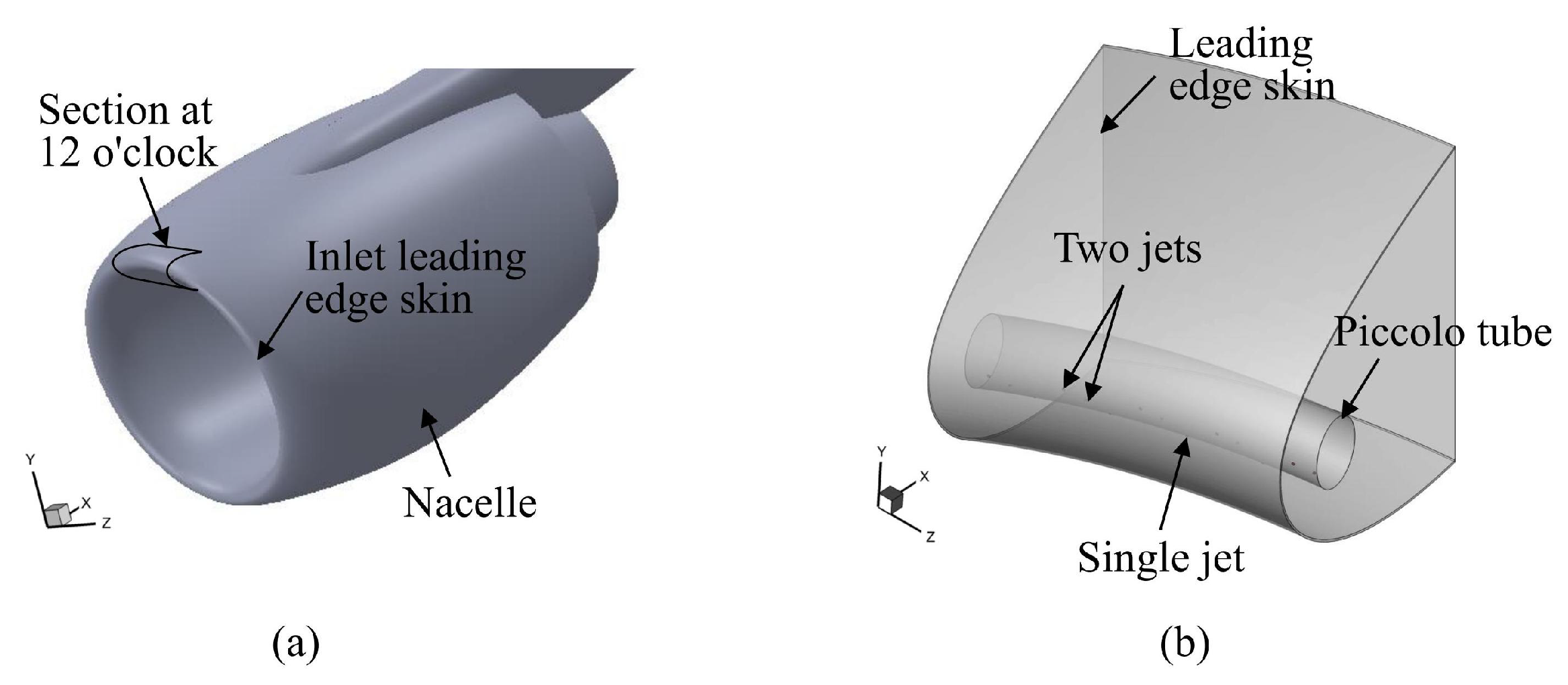
Figure 2.
Design variables of inlet hot-air anti-icing system.
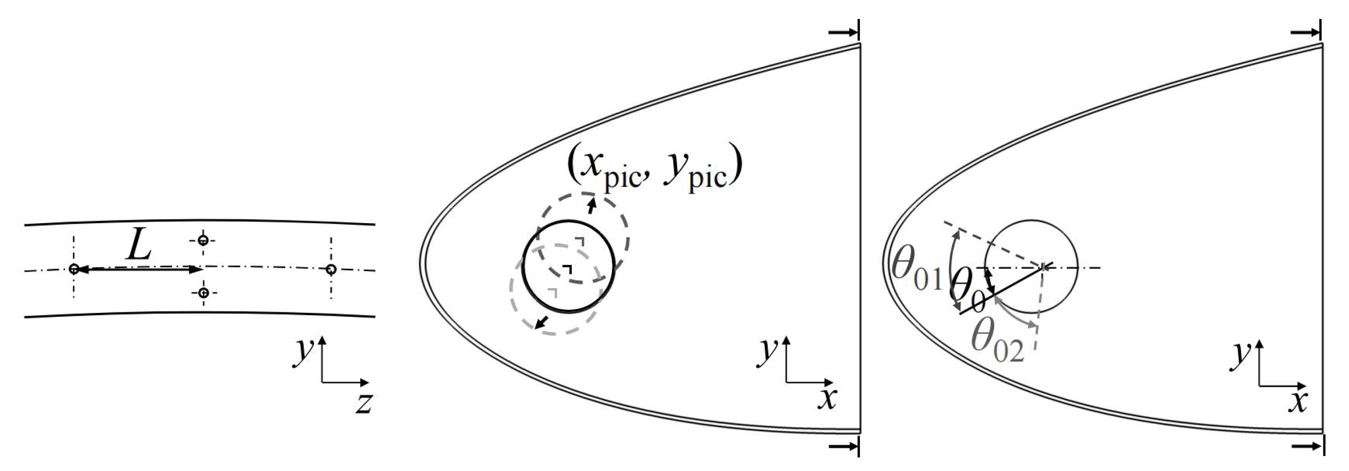
Figure 3.
Structured mesh of inlet hot-air anti-icing system skin.
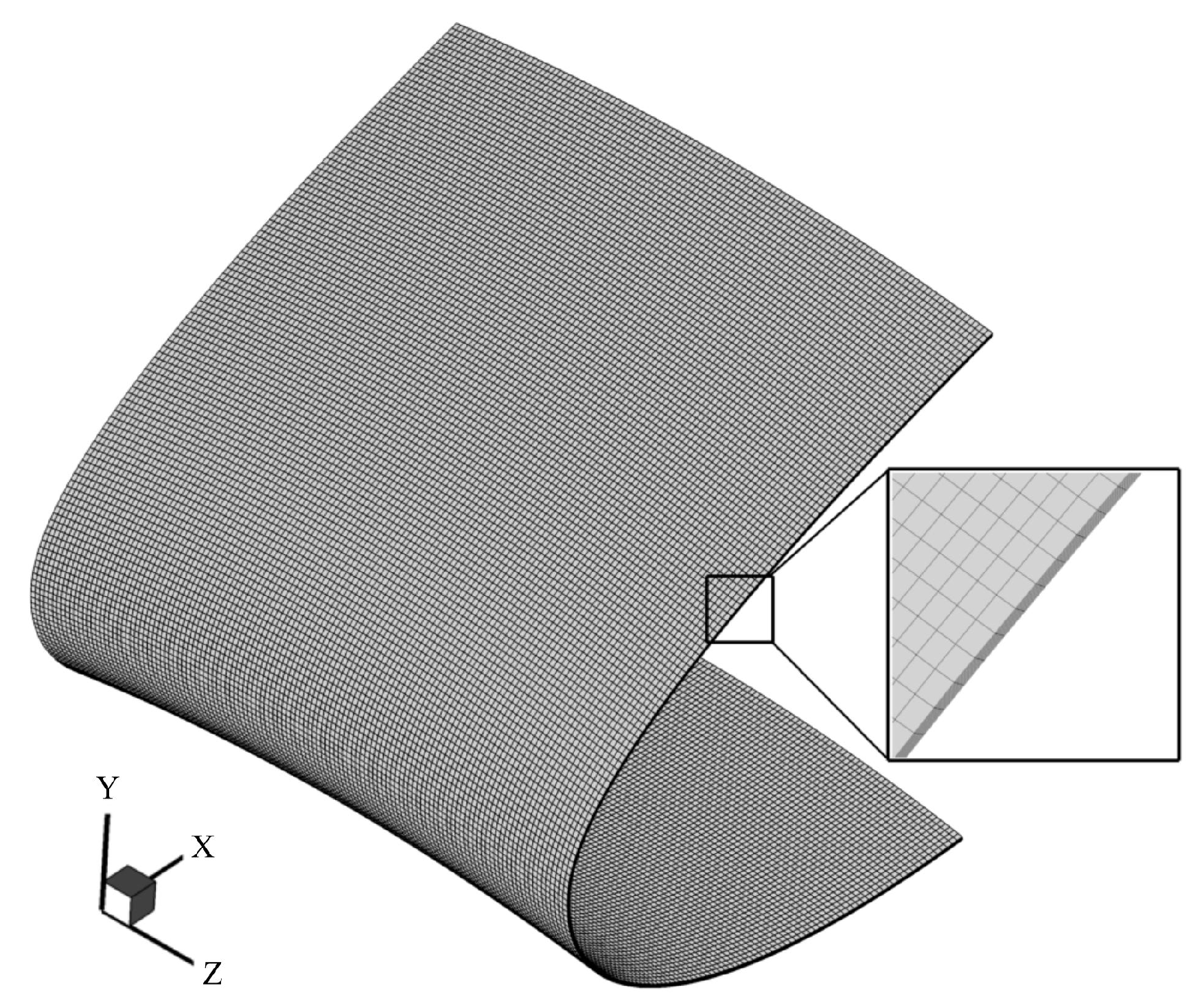
Figure 4.
Structure of AlexNet suggested by [22].
Figure 4.
Structure of AlexNet suggested by [22].
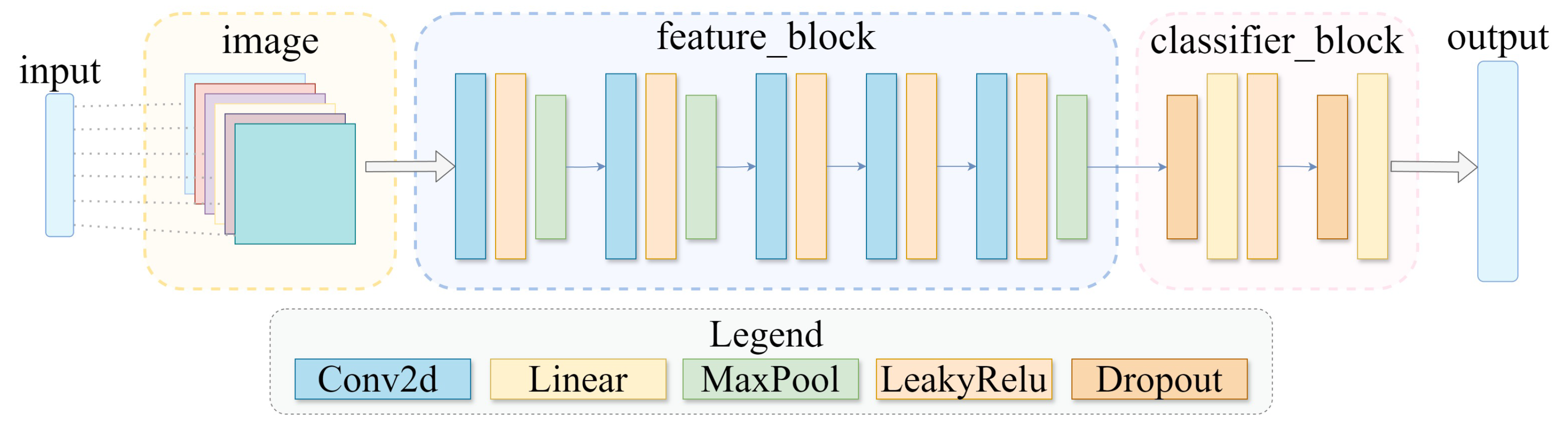
Figure 5.
Structure of GRU suggested by [27].
Figure 5.
Structure of GRU suggested by [27].
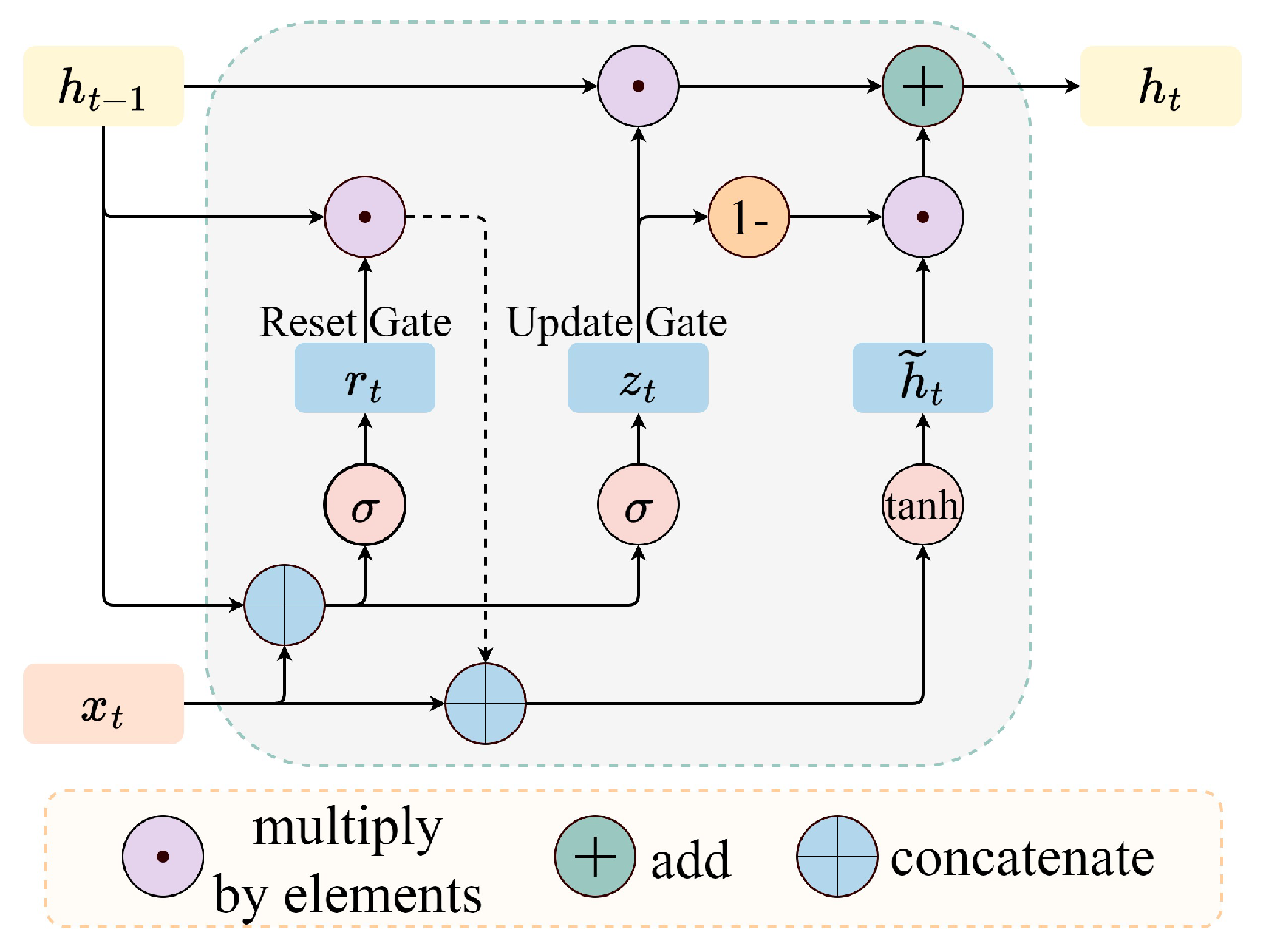
Figure 6.
The technical workflow diagram.
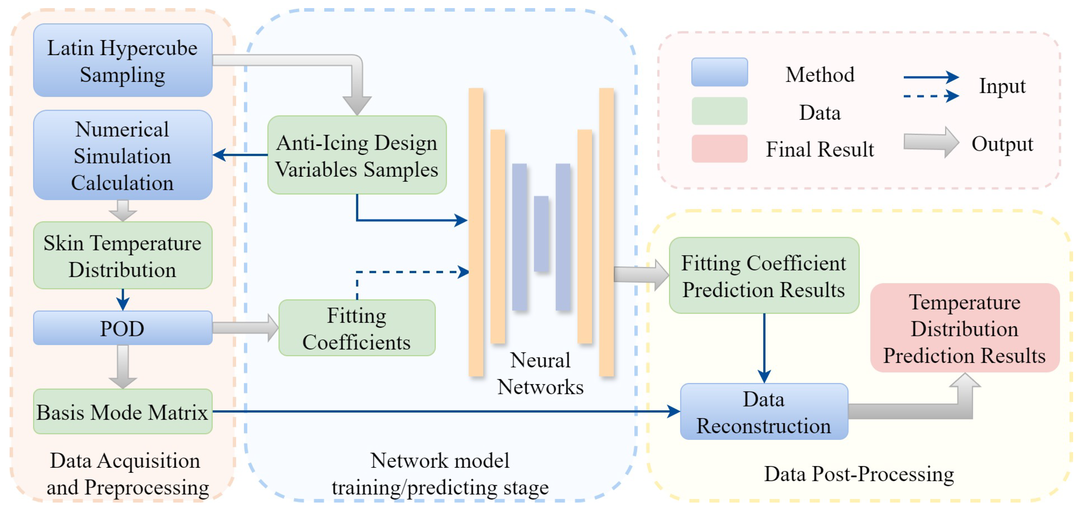
Figure 7.
The curve of energy ratio relative to the number of POD modes.
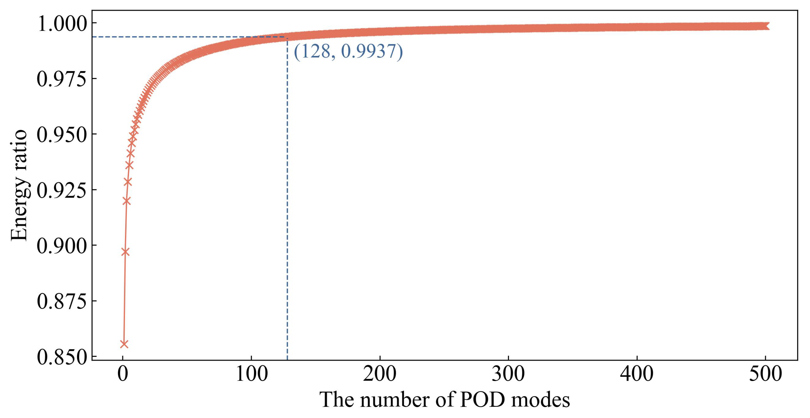
Figure 8.
The data flow diagram.
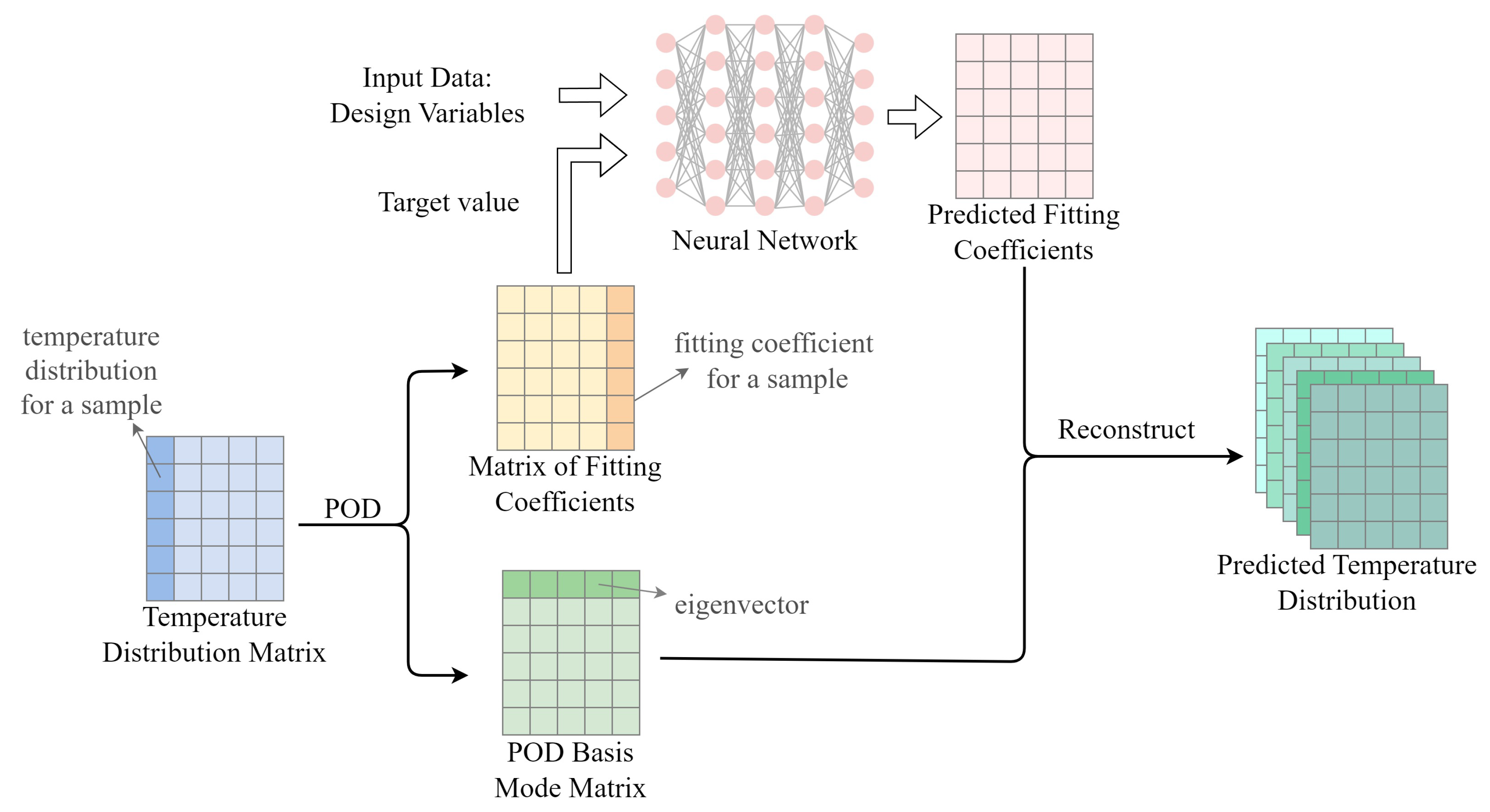
Figure 9.
The network structure of MCG.
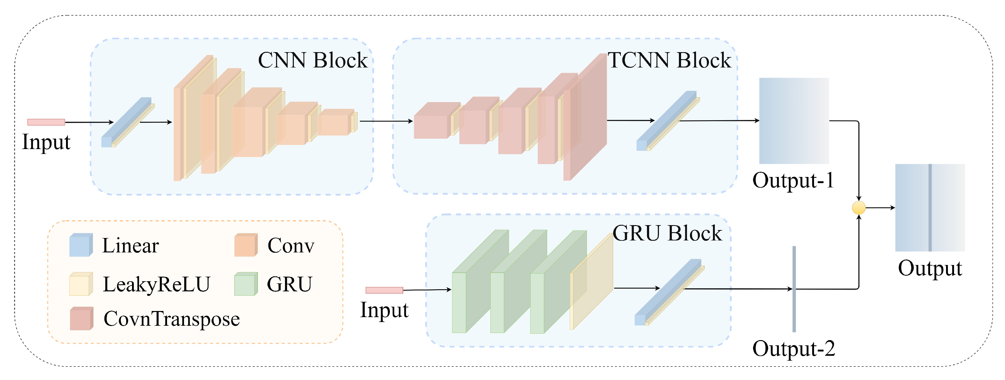
Figure 10.
The variation in loss values during the ROM training process.
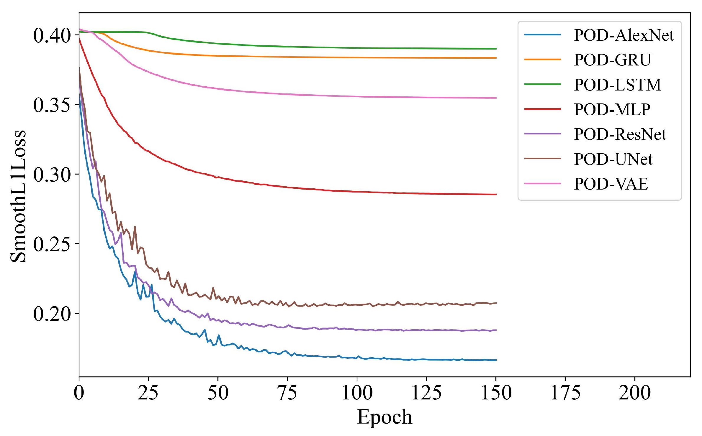
Figure 11.
Comparison between target results and predicted results of POD-AlexNets. (a) Comparision of testing sample #50; (b) comparision of testing sample #210; (c) comparision of testing sample #225; (d) comparision of testing sample #428.
Figure 11.
Comparison between target results and predicted results of POD-AlexNets. (a) Comparision of testing sample #50; (b) comparision of testing sample #210; (c) comparision of testing sample #225; (d) comparision of testing sample #428.
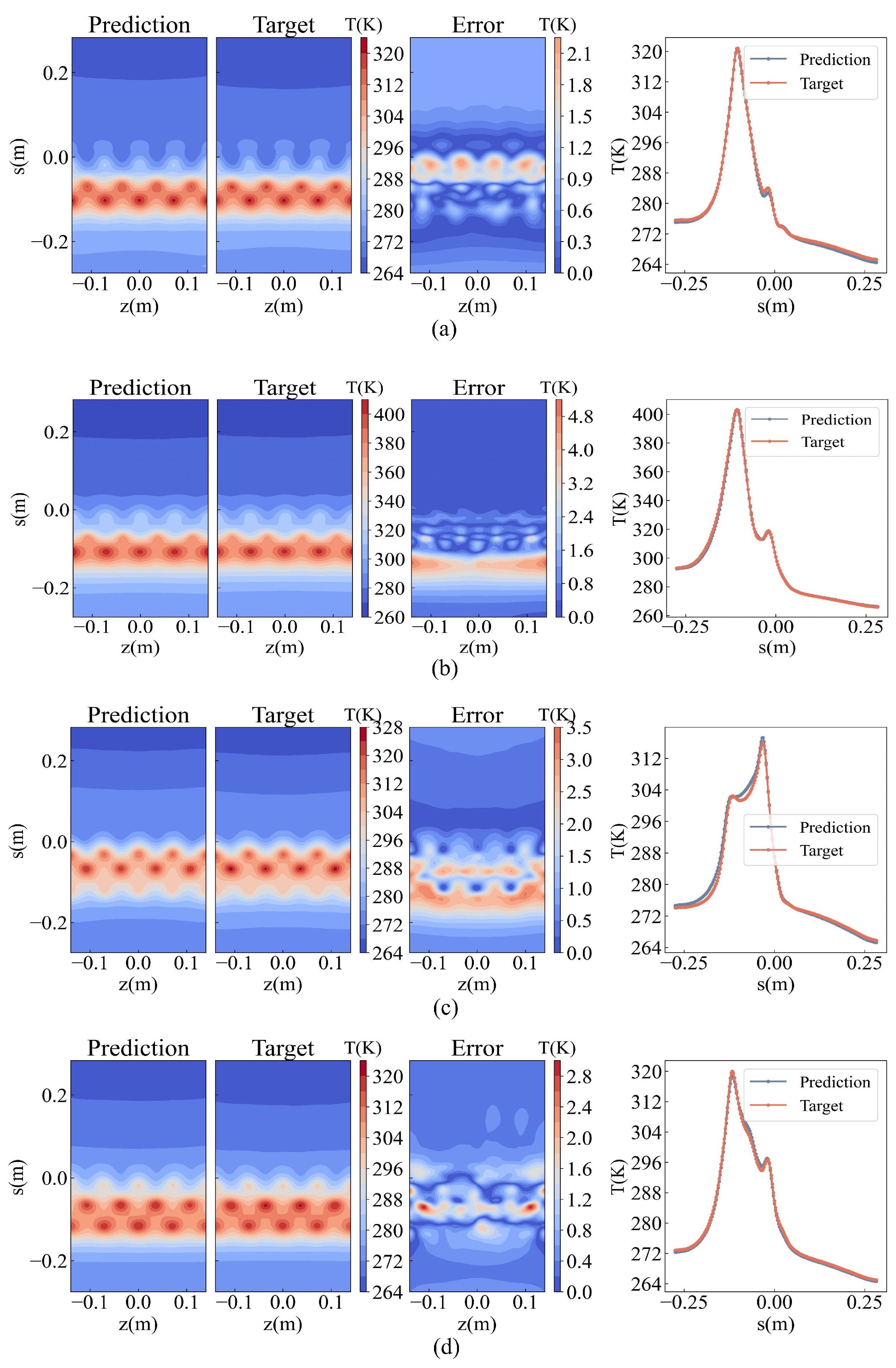
Figure 12.
The variation in loss values during the high-dimensional model training process.
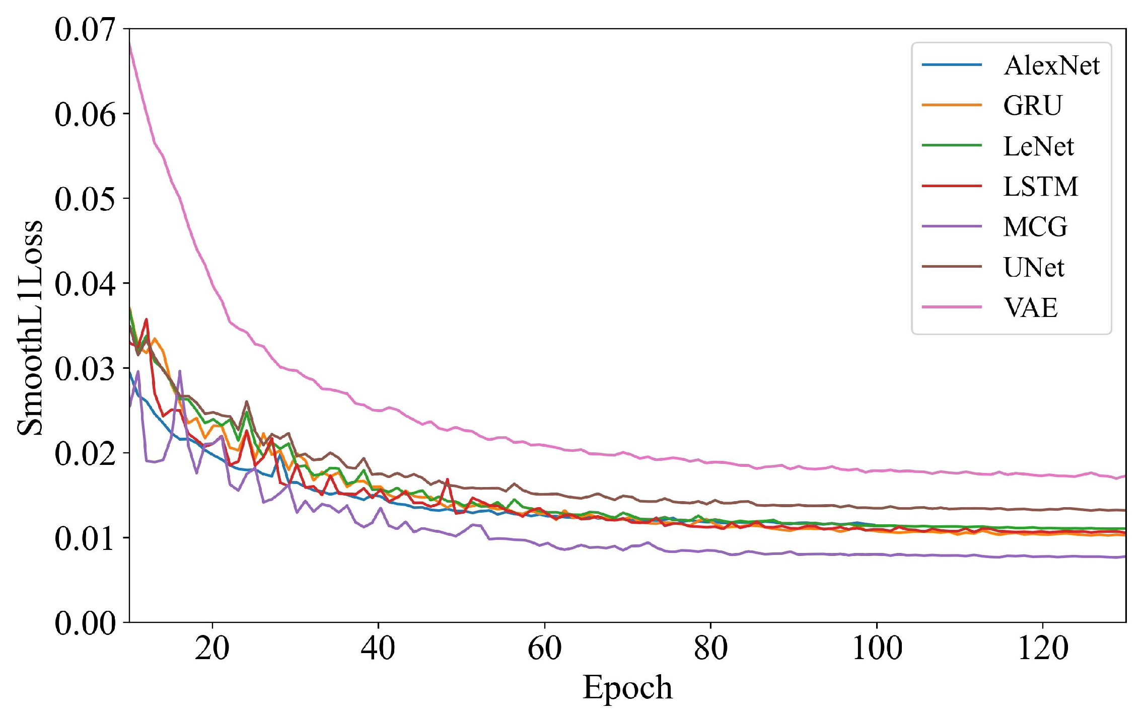
Figure 13.
Comparison between target results and predicted results of MCG. (a) Comparision of testing sample #50; (b) comparision of testing sample #210; (c) comparision of testing sample #225; (d) comparision of testing sample #428.
Figure 13.
Comparison between target results and predicted results of MCG. (a) Comparision of testing sample #50; (b) comparision of testing sample #210; (c) comparision of testing sample #225; (d) comparision of testing sample #428.
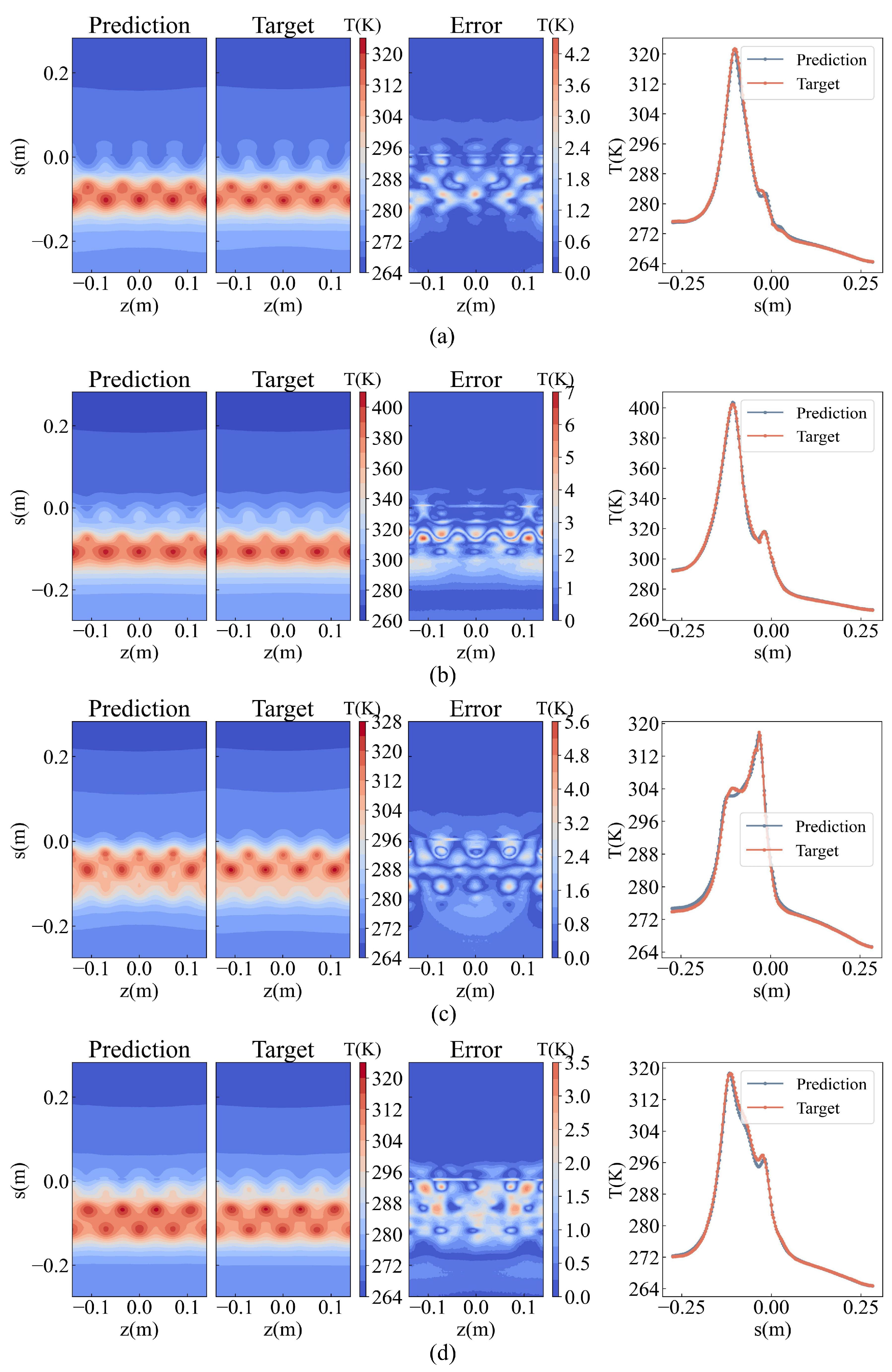
Figure 14.
Absolute error of POD-AlexNet and MCG. (a) Comparision of testing sample #50; (b) comparision of testing sample #210; (c) comparision of testing sample #225; (d) comparision of testing sample #428.
Figure 14.
Absolute error of POD-AlexNet and MCG. (a) Comparision of testing sample #50; (b) comparision of testing sample #210; (c) comparision of testing sample #225; (d) comparision of testing sample #428.
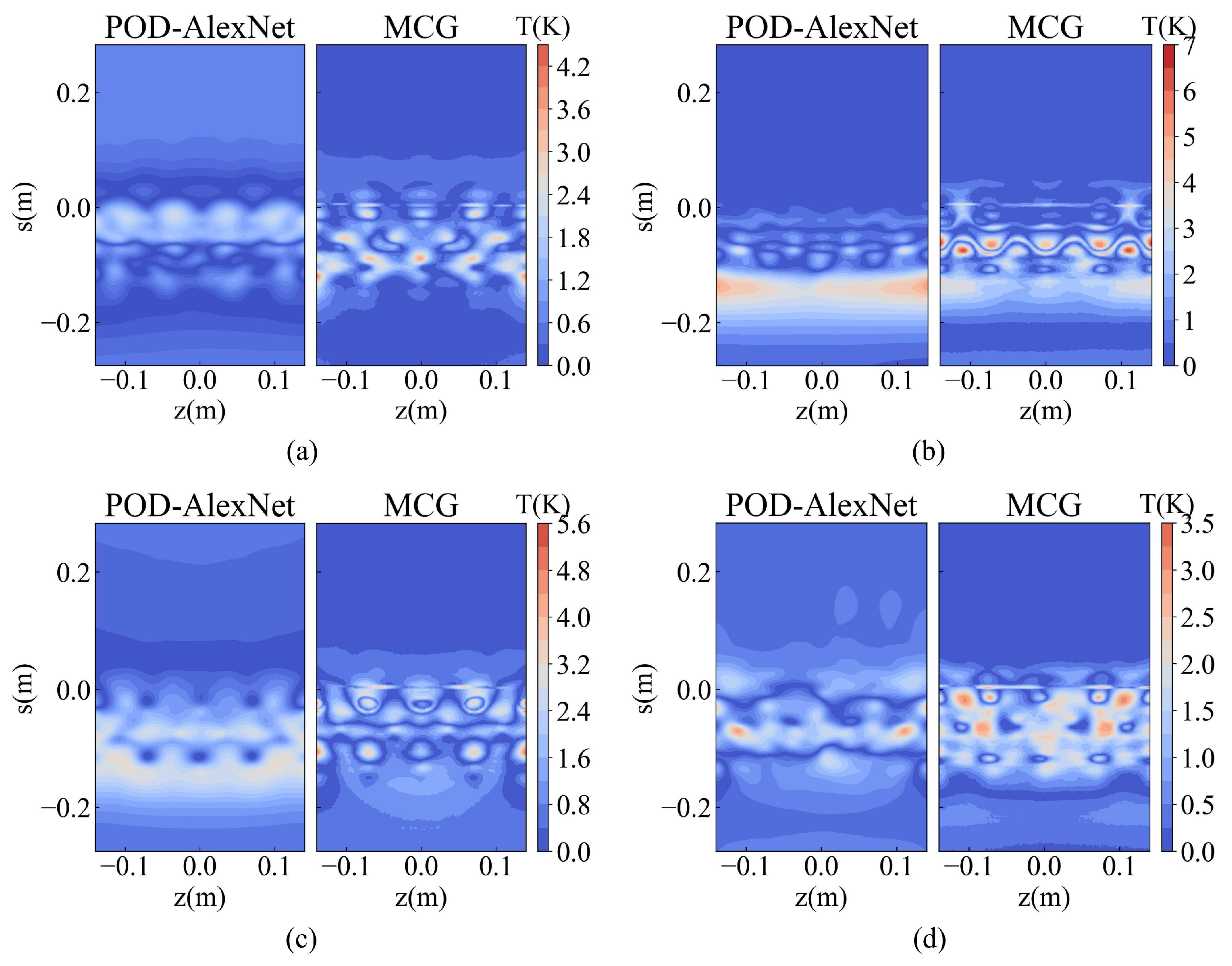

Table 1.
The range of design variables for inlet hot-air anti-icing system.
| Design variables | L/D | /D | /D | / | / | / |
|---|---|---|---|---|---|---|
| Baseline | 14.6 | 0 | 0 | 1 | 0.86 | 0.73 |
| Range | [10,20] | [-10,7.5] | [-10,7.5] | [0.54,1.08] | [0.54,1.08] | [0.54,1.08] |
Table 2.
Design conditions for inlet hot-air anti-icing system.
| H | AoA | Ma | MVD | LWC | ||||
|---|---|---|---|---|---|---|---|---|
| 6 km | 4° | 0.427 | 263.55 K | 20 m | 0.43 g/ | 0.25 MPa | 555 K | 1.33 g/s |
Table 3.
Performance evaluation results of methods based on ROM.
| Networks | |||||
|---|---|---|---|---|---|
| POD-MLP | 3.27 | 0.80% | 2.44 | 88.25% | 4.0ms |
| POD-LSTEM | 11.19 | 2.46% | 7.74 | 57.28% | 0.7ms |
| POD-GRU | 8.98 | 2.07% | 6.45 | 58.81% | 0.4ms |
| POD-VAE | 4.16 | 0.93% | 2.87 | 83.57% | 0.4ms |
| POD-UNet | 4.41 | 1.15% | 3.43 | 78.48% | 1.2ms |
| POD-ResNet | 2.81 | 0.69% | 2.11 | 90.86% | 0.5ms |
| POD-AlexNet | 1.99 | 0.47% | 1.45 | 95.83% | 1.0ms |
Table 4.
Performance evaluation results of methods based on high-dimensional model.
| Networks | |||||
|---|---|---|---|---|---|
| LeNet | 2.85 | 5.26‰ | 1.66 | 91.76% | 7.5ms |
| AlexNet | 2.80 | 4.98‰ | 1.59 | 92.23% | 8.5ms |
| UNet | 2.84 | 5.26‰ | 1.66 | 91.82% | 1.3ms |
| VAE | 3.62 | 6.40‰ | 2.05 | 88.46% | 4.6ms |
| LSTM-3L | 2.56 | 4.68‰ | 1.48 | 93.18% | 5.4ms |
| GRU-3L | 2.47 | 4.56‰ | 1.45 | 93.64% | 5.5ms |
| MCG | 1.75 | 3.23‰ | 1.02 | 96.97% | 5.5ms |
Disclaimer/Publisher’s Note: The statements, opinions and data contained in all publications are solely those of the individual author(s) and contributor(s) and not of MDPI and/or the editor(s). MDPI and/or the editor(s) disclaim responsibility for any injury to people or property resulting from any ideas, methods, instructions or products referred to in the content. |
© 2024 by the authors. Licensee MDPI, Basel, Switzerland. This article is an open access article distributed under the terms and conditions of the Creative Commons Attribution (CC BY) license (http://creativecommons.org/licenses/by/4.0/).
Copyright: This open access article is published under a Creative Commons CC BY 4.0 license, which permit the free download, distribution, and reuse, provided that the author and preprint are cited in any reuse.


