
Submitted:
21 October 2024
Posted:
23 October 2024
You are already at the latest version
Abstract
This research presents a novel methodology for classifying MRI images into two categories: tumor and non-tumor. The study utilizes a combination of two advanced Convolutional Neural Network (CNN) architectures, VGG16 and ResNet50, to address the challenges in analyzing the complexity and variability of brain MRI scans. The approach begins with a comprehensive preprocessing phase, where the MRI images are enhanced through techniques such as resizing, grayscale conversion, Gaussian blurring, and brain area isolation. Central to the approach is the application of the Multi-verse Optimizer (MVO), a metaheuristic algorithm inspired by theories of the multi-verse in physics. The MVO is utilized to optimize the parameters for data augmentation and to fine-tune the combination of trainable layers within the VGG16 and ResNet50 models. The results of this study indicate a high level of effectiveness of the combined CNN models, significantly enhanced by the MVO, in classifying MRI images. These models show marked improvements in accuracy, precision, and recall, underscoring their potential utility in enhancing brain tumor diagnosis. The paper concludes with an analysis of these findings, emphasizing the importance of this approach in medical imaging and suggesting potential avenues for future research in the area of automated MRI classification.
Keywords:
Brain Tumor Classification
; MRI Image Analysis
; Optimization
; Deep Learning
; Data Augmentation
; Multi-verse Optimizer
1. Introduction
Brain tumors, one of the most daunting medical diagnoses, present a formidable challenge in healthcare. These abnormal cell growths in the brain can have devastating effects on health and well-being [1,2,3]. Early and accurate recognition is paramount for effective treatment planning and improved prognosis. Traditionally, the diagnosis of brain tumors relies heavily on the analysis of MRI images by experts or radiologists. However, this manual process is not only labor-intensive but also prone to human error. The advancement of automated classification methods, particularly through machine learning, offers a transformative solution, promising greater accuracy, efficiency, and consistency in diagnosing brain tumors [4,5,6].
Machine learning (ML), a subgroup of artificial intelligence (AI), involves the development of techniques that enable computers to learn from data and make decisions without being explicitly programmed. It encompasses numerous methods that allow systems to improve automatically through experience, making it a powerful tool for interpreting and analyzing vast amounts of data [7,8,9,10,11,12,13,14].
In contemporary applications, supervised models based on ML have become integral to a wide range of applications. They are prominently employed in natural language processing (NLP), where they help in understanding and interpreting human languages with applications ranging from translation services to sentiment analysis [15,16]. In the medical field, these techniques are revolutionizing medical image processing, enabling more precise diagnoses from imaging data, and also enhancing medical signal processing for better monitoring and treatment of health conditions [6,17,18,19,20]. The widespread adoption of ML models in diverse fields underscores their versatility and transformative potential in technology and science [8,10,21,22].
In the field of automated brain tumor classification, two main ML methodologies have emerged as predominant methods: hand-crafted feature extraction methods and deep learning (DL) methods. Each technique offers distinct strategies and benefits for the analysis and classification of brain tumors from MRI images [23,24,25].
Hand-crafted feature extraction relies on predefined strategies to identify specific characteristics or 'features' in MRI images. These features, such as intensity, shape, and texture, are then utilized to classify the images into tumor or non-tumor categories. While these methods have been instrumental in early efforts at automated classification, they are limited by the need for expert knowledge in feature selection and can struggle with the high variability present in brain tumor images [4,6,26].
Leveraging neural networks, particularly CNNs, DL models automatically learn feature descriptions directly from the data, bypassing the need for manual feature extraction. These approaches have shown remarkable success in various image recognition tasks, including medical image analysis. CNNs, with their ability to hierarchically extract and learn complicated hidden patterns in data, have become the cornerstone of modern automated image classification, including the differentiation of MRI images into tumor and non-tumor categories [5,27,28,29,30,31,32].
Vankdothu et al. [33] developed an innovative automated system for detecting and classifying medical images. This system encompasses several stages: preprocessing of MRI images, segmentation, feature extraction, and classification. In the preprocessing stage, an adaptive filter is applied to reduce noise in the MRI images. For image segmentation, an enhanced version of the K-means clustering technique, known as IKMC, is utilized. The feature extraction procedure utilizes the gray-level co-occurrence matrix (GLCM) strategy to draw out critical and hidden patterns from the images. Subsequently, these features are input into a DL model for classification into various categories, such as non-tumors, meningiomas, gliomas, and pituitary tumors, utilizing recurrent CNNs (RCNN). This strategy demonstrated improved outcomes in classifying brain images from a specific dataset. The evaluation of this method was carried out using a dataset from Kaggle, comprising 394 test images and 2870 training images. The findings indicate that this method outperforms previous approaches in terms of performance. Additionally, the effectiveness of the RCNN model was benchmarked against contemporary classification techniques like U-Net, backpropagation, and RCNN, showcasing its superior capabilities in medical image classification.
Siddiqi et al. [34] suggested a cutting-edge feature extraction technique specifically designed for MRI images, aimed at identifying and selecting prominent features associated with different brain diseases. This strategy stands out for its ability to discern key features from MRI scans, facilitating the differentiation between various disease classes. The approach employs a novel method that utilizes recursive values like the partial Z-value for class discrimination. The algorithm works by extracting a select set of features through backward and forward recursion models. In the forward recursion model, the most interrelated features are identified based on the partial Z-test values. Conversely, the backward model aims to decrease the least interrelated features from the feature space. In both instances, the Z-test values are computed based on the predefined labels of the diseases, aiding in the precise identification of localized features, which is a major advantage of this method. Once the optimal features are extracted and selected, the model employs a Support Vector Machine (SVM) for training. This training allows the model to assign predictive labels to the MRI images accurately.
Ullah et al. [35] proposed a theory emphasizing the critical role of image quality, particularly when enhanced during the preprocessing phase, in improving the classification accuracy of statistical methods. To support this theory, they introduced an advanced image enhancement procedure comprising three distinct sub-stages. Initially, noise is mitigated using a median filter, followed by the enhancement of image contrast through histogram equalization. The process culminates with the conversion of images from grayscale to RGB. Once the images are enhanced, feature extraction is conducted on the improved MR brain images employing discrete wavelet transform. These extracted features are then further processed by implementing color moments, which include skewness, mean, and standard deviation, to effectively reduce the feature set. The final step involves training an advanced Deep Neural Network (DNN) with these processed features. The purpose of this DNN is to correctly classify human brain MRI images, differentiating between normal and pathological conditions. This approach underscores the significance of image quality in preprocessing and its impact on the efficacy of DL models in medical imaging classification tasks.
Alrashedy et al. [36] introduced BrainGAN, a framework designed for both generating and classifying brain MRI images. This framework utilizes Generative Adversarial Network (GAN) architectures alongside DL models. A key aspect of this study was the development of an automated technique to ensure the quality of images generated by GANs. For this purpose, the framework used three different models: MobileNetV2, CNN, and ResNet152V2. These deep transfer models were trained employing images generated by two types of GANs: Deep Convolutional GAN (DCGAN) and Vanilla GAN. The effectiveness of these models was then assessed using a test set comprised of actual brain MRI images. The experimental results indicated that the ResNet152V2 model exhibited superior performance compared to the CNN and MobileNetV2 models. This outcome underscores the potential of using advanced neural networks in conjunction with GAN-generated data for the accurate classification of medical images, especially in scenarios where real-world data is limited or difficult to access.
Our study introduces a comprehensive model that harnesses the power of DL for the classification of brain MRI images into tumor and non-tumor categories. We employ a sophisticated strategy that combines the strengths of two renowned CNN architectures, VGG16 and ResNet50. These models have been selected for their proven efficacy in image classification tasks, providing a robust foundation for our classification strategy.
The proposed approach begins with a critical preprocessing phase, pivotal for preparing MRI images for analysis by CNN models. This part incorporates several procedures, including image resizing, conversion to grayscale, and the application of Gaussian blurring. These processes are instrumental in minimizing noise and standardizing the images, ensuring the focus is on features crucial for classification. Further, advanced image processing techniques are utilized to accurately isolate the brain region from each scan, a key step in precise tumor detection.
An innovative optimization technique is integrated into the model development, employing the Multi-verse Optimizer (MVO). A significant application of MVO in this study is the optimization of data augmentation parameters. Data augmentation is an essential step in enhancing the robustness and generalization of DL models. By artificially enlarging the training dataset with modified versions of original images, the risk of overfitting is diminished. This also prepares the models to manage diverse image variations. MVO plays a critical role in identifying the most effective augmentation techniques and their parameters, optimizing the process for brain MRI images.
Furthermore, MVO is instrumental in determining the optimal configuration of trainable layers in the VGG16 and ResNet50 architectures, a crucial factor in adapting the models for brain tumor classification. The selective unfreezing of layers for training achieves a balance between employing pre-learned features and adapting to the specific dataset. MVO directs this process, identifying layers that, when trained, significantly boost the model's efficacy.
The structure of this paper is accurately organized to offer a comprehensive understanding of the methodology and results. The introduction is followed by the materials and methods section, which details the preprocessing steps and the MVO optimization process. Following this, the data augmentation strategies and the process of building and training the VGG16 and ResNet50 models are thoroughly examined. The model evaluation section follows, discussing the metrics and techniques utilized to assess the performance of the models. A critical analysis of the findings is presented in the results and discussion section, where the effectiveness of this approach is compared with other methods, particularly emphasizing its role in the automated detection of brain tumors. The paper concludes with a summary of the key contributions and insights, and it outlines potential future research avenues in this crucial area of medical diagnostics.
2. Materials and Methods
This section methodically outlines the proposed method. Initially, the visual summary of the recommended model is illustrated in Figure 1.
2.1. Data Preprocessing
The preprocessing of MRI images is a fundamental step towards achieving accurate classification results when discerning between scans with and without tumors. Our procedure is designed to extract just the brain region from each MRI image, utilizing a combination of image processing techniques provided by the OpenCV library. These steps are described as follows:
- Image Resizing: Each image is resized to a standard dimension, certifying uniformity across the dataset. This is important for consistency when feeding the images into the neural network models.
- Grayscale Conversion: The resized images are converted to grayscale to moderate computational complexity. Color information is typically redundant for the task at hand, as the focus is on texture and shape within the images.
- Gaussian Blurring: To reduce high-frequency noise, a Gaussian blur is applied to the grayscale images. This smoothing technique aids in highlighting the more significant structures within the brain by softening edges and details.
- Otsu's Thresholding: We implement Otsu's thresholding to separate the brain tissue from the background. This method automatically computes a threshold value for image binarization, which is employed to detect contours.
- Contour Detection and Selection: By applying contour detection, we identify the boundaries of all the objects in the binary image. We assume the largest contour to be the brain's boundary, a reasonable assumption in a typical MRI scan.
- Extreme Points and Cropping: Once the largest contour is identified, we verify its extreme points. These points represent the furthest pixels in the horizontal and vertical directions within the contour, which we employ to define a cropping boundary.
- Image Cropping: The image is cropped using the extreme points as vertices, with an optional padding added to ensure no part of the brain is excluded.
- Displaying the Process: We visualize the preprocessing steps, displaying the original image, the contour of the largest detected region, the extreme points, and finally, the cropped brain region.
It is important to note that the performance of this preprocessing step depends on the characteristics and quality of the MRI scans provided. If the scans are not standardized or contain artifacts, additional preprocessing techniques might be required. Figure 2, demonstrates the results of applying the proposed preprocessing method.
2.2. Optimization Method
Optimization in ML is the manipulation of model parameters in order to minimize errors and enhance the precision of predictions. It's a vital process in model training that directly affects the performance of the model [11,17,37,38]. Metaheuristics are high-level problem-independent algorithmic frameworks that provide a set of guidelines or approaches to developing heuristic optimization algorithms. They are often nature-inspired and designed to investigate the search space efficiently, which is crucial in avoiding local optima and finding a near-global optimum in complex problems. Unlike exact techniques, metaheuristics do not guarantee an optimal solution, but they often discover good solutions with less computational effort, especially in large and complex search spaces [39,40,41,42,43].
In our study, we utilized the MVO technique, an effective metaheuristic algorithm inspired by the multi-verse theory in physics. The MVO algorithm models each solution as a universe and the features of the solutions as objects within these universes. The algorithm iterates through a process of exploration and exploitation, guided by the concepts of wormholes, black holes, and white holes, to share information among the universes and converge towards the best solution [44,45,46]. White Holes act as channels for exporting matter from a universe, which in MVO terms, means exporting solution features from a higher-ranked solution to others. Black Holes serve the opposite function, absorbing matter, and thus importing solution features from other universes into the current solution. Wormholes provide a means for solutions to jump across the search space, encouraging exploration and aiding in avoiding local minima [44,47,48].
We used the MVO method for two main optimization tasks:
- Optimization of Data Augmentation Parameters: MVO was utilized to uncover the best data augmentation techniques and their respective parameter values. This step was crucial to enhance the dataset variability without deviating from the realistic transformations applicable to MRI images. By doing so, we aimed to maximize the performance of the classification models while avoiding overfitting.
- Layer-wise Trainability in CNNs: We also applied the MVO strategy to find the optimal configuration of trainable layers within VGG16 and ResNet50 architectures. The method helped in identifying which layers should be frozen (weights not updated during training) and which should be trainable (weights updated during training) to improve the models' accuracy and efficiency. This is particularly important as deep neural networks can be computationally expensive to train, and freezing certain layers can significantly diminish the number of parameters that essential to be updated, thus speeding up the training process and potentially improving generalization.
The MVO relies on various parameters that guide the optimization process. Adjusting these parameters can notably influence the algorithm's ability to find optimal solutions. Below is a detailed description of these parameters and the role they play in the MVO algorithm [46,47,48]:
- Universe Size (Population Size): This parameter defines the number of potential solutions (universes) that the algorithm will consider simultaneously. A larger universe size allows for greater exploration of the solution space. A universe size of 30 achieves a compromise between computing efficiency and diversity within the search space. More extensive populations enhance diversity but may impede the optimization process, whereas smaller populations might converge rapidly yet risk overlooking ideal solutions due to inadequate research. A universe size of 30 facilitates a sufficiently diversified population to investigate many solutions while minimizing computational expenses.
- Wormhole Existence Probability (WEP): This probability controls the creation of wormholes, which are mechanisms for sharing information between universes. A value of 0.6 signifies a considerable probability of the formation of these wormholes. This likelihood facilitates an effective combination of exploration (investigating new regions of the solution space) and exploitation (enhancing current solutions). A high WEP (approaching 1) may result in premature convergence due to excessive emphasis on exploitation, whereas a low WEP (approaching 0) restricts exploitation, hence obstructing convergence to an ideal solution. A WEP of 0.6 guarantees that the MVO algorithm can efficiently navigate the solution space while simultaneously enhancing viable solutions.
- Travelling Distance Rate (TDR): This rate determines how much a solution can be altered when a wormhole event occurs. A value of 0.4 signifies that alterations to the solutions are moderate. If the TDR is overly elevated, solutions may be excessively disturbed, resulting in irregular exploration that could overlook excellent solutions. If TDR is excessively low, the algorithm may adopt an overly conservative approach and become trapped in local optima. A TDR of 0.4 offers a balanced methodology, enabling the algorithm to implement significant modifications to solutions while remaining close to attractive regions.
- Maximum/Minimum WEP: These parameters set the lower and upper bounds for the wormhole existence probability, introducing dynamic variability in the algorithm. The interval [0.2, 1.0] guarantees that during the initial phases of optimization, the method prioritizes exploration (with a reduced WEP at 0.2), so avoiding premature convergence. As the algorithm advances, WEP approaches 1.0, highlighting exploitation in the latter phases to optimize the results. The incremental rise in WEP enables the early investigation of several options, while refining the search in the concluding iterations for enhanced precision.
- Maximum/Minimum TDR: Similar to WEP, these parameters set the boundaries for the travelling distance rate, controlling the extent of solution alterations through the optimization process. Commencing with a minimum TDR of 0.4 guarantees that initial exploration remains closely aligned with the existing optimal solutions. As optimization progresses, the TDR may rise to 1.0, facilitating more substantial alterations in subsequent phases. This adaptive modification allows the method to maintain flexibility throughout the initial phases of optimization, while intensifying solution refinement as it nears convergence.
These parameters are not static; they can be adapted during the optimization process to dynamically adjust the search behavior of the method. For the purpose of our study, Table 1 outlines the specific parameters of the MVO algorithm that were employed to optimize data augmentation techniques and determine trainable layers in the VGG16 and ResNet50 models:
2.3. Data Augmentation
Data augmentation is an essential strategy in the field of DL, especially when dealing with image data. It refers to the process of generating new training samples from the original ones by applying sequence of random changes that result in realistic variances [49,50,51]. This technique is crucial for several reasons [49,50,52]:
- Mitigates Overfitting: Augmentation spreads the variety of the training samples, which helps in preventing the model from memorizing specific images and overfitting.
- Improves Generalization: By simulating various scenarios, data augmentation allows the model to generalize better to new, unseen data.
- Compensates for Imbalanced Datasets: In cases where some classes are underrepresented, augmentation can help to balance the samples without the need to collect more data.
- Enhances Model Robustness: Augmented data aids the model to learn more robust features that are invariant to certain transformations, which is significant for real-world applications.
In our study, the ‘ImageDataGenerator’ from ‘Keras’ is used to implement data augmentation, with a range of parameters set to apply random transformations to the images. Table 2 summarizes the data augmentation approaches employed in our study. Figure 3 demonstrates the results of applying the augmentation methods to an image.
2.4. Model Building with VGG16 and ResNet50
In our study, we focused on building and fine-tuning two prominent CNN architectures: ResNet50 and VGG16. These models were chosen for their proven track records in image classification tasks.
VGG16 stands out for its depth and utilize of uniform 3x3 convolutional layers. Its architecture is a demonstration to the idea that depth is crucial for attaining high levels of accuracy in complex image classification tasks. A pre-trained VGG16 model, originally trained on the ImageNet dataset, provides a strong feature extraction base due to its exposure to a widespread variety of images. However, this model is often criticized for its high computational cost and extensive memory requirement, mainly due to its deep architecture and fully connected layers [53,54,55,56,57].
The adaptation of VGG16 for binary classification involves fine-tuning the dense layers to suit the specific task. The main advantage here is the ability to capture fine-grained details, which can be necessary for discovering subtle features in MRI images indicative of tumors.
ResNet50, with its residual blocks and skip connections, addresses the challenge of training deep networks without falling prey to the vanishing gradient problem. The skip connections facilitate the training of the model by letting gradients to flow through the architecture more effectively. A pre-trained ResNet50 model brings robustness and a quicker training convergence to the table, owing to these residual blocks. The architecture is more efficient than VGG16, both in terms of computational resources and required training time, making it a strong candidate for DL tasks. However, one could argue that ResNet50 may sometimes lead to feature redundancy due to its very deep architecture [52,58,59,60,61].
In the binary classification of MRI images, ResNet50's architecture is beneficial for its ability to learn from residuals, potentially refining the model's ability to distinguish relevant patterns associated with tumors.
Combining ResNet50 and VGG16 can be particularly advantageous for the task at hand. While VGG16 is adept at capturing texture and detailed features, ResNet50 excels in leveraging deeper contextual information and solving the degradation problem in deep networks. The fusion of these models could lead to a comprehensive feature extraction mechanism, where VGG16 contributes detailed local features and ResNet50 contributes broader contextual understanding.
This combined methodology may offer a more robust representation of the MRI images, capturing both the minute details essential for distinguishing small or early-stage tumors and the broader patterns necessary for identifying more significant anomalies. The ensemble of these two architectures has the potential to capitalize on the strengths of both while mitigating their individual weaknesses, leading to an improved classification performance.
2.5. Model Training
The model training phase was characterized by a dynamic and adaptive method. Each training iteration was contingent upon the new sets of hyperparameters recommended by the optimization process for data augmentation and layer unfreezing. This strategy ensured that the training process was continually refined and tailored based on the model's performance feedback.
The iterative nature of the training was closely tied to the MVO, which provided updated values for data augmentation parameters and discovered the layers to be unfrozen for each training cycle. This method permitted the model to evolve in conjunction with the optimizer's findings, effectively creating a feedback loop between training performance and parameter adjustment.
The optimizer's role was essential in defining the non-trainable and trainable parameters of the model. With a total of 102,659,777 parameters, the optimizer fine-tuned the model by selectively unfreezing layers. This strategic balance played a substantial role in the model's ability to adapt to the specific features of MRI images.
Data augmentation was not a static preprocessing phase but a variable aspect of training. As the optimizer advocated new augmentation values, the training samples was transformed accordingly, which permitted the model to learn from a more diverse set of features. This continual alteration of the training samples helped mitigate overfitting and improved the model's generalizability.
During each training iteration, the structure was assessed using a validation set to monitor its performance against data that was not part of the training process. This regular validation served as a checkpoint to verify the efficacy of the current set of hyperparameters and informed subsequent adjustments from the optimizer.
Throughout the training phase, the model underwent evolution, not only in its biases and weights but also in its structure as layers were unfrozen and data augmentation techniques were varied. This evolution aimed to refine the model's capability to identify and classify the presence of tumors in MRI scans with increasing precision.
The outcome of this iterative and adaptive training process was a highly tuned model, uniquely customized to the task at hand. The model's training was directly influenced by the optimizer, confirming that with each training cycle, the model was progressively equipped to handle the complexities of tumor detection in MRI images.
2.6. Dataset
The employed dataset consists of 3,264 brain MRI scans [62]. These scans are derived from individuals seeking medical assessment and evaluation of their brain health. Each MRI scan holds the potential to reveal critical information about the presence or absence of brain tumors. MRI, being non-invasive, ensures minimal discomfort and risk to the patients while delivering invaluable insights into the brain's intricate anatomy. We utilized 10% of samples for validation, 10% of samples for test, and the rest for the training purpose. Some images from the dataset are indicated in Figure 4.
The dataset is carefully labeled, attributing two distinct classes to each MRI scan [62]:
-
No Tumor:
- This class encompasses brain MRI scans attained from individuals who do not demonstrate any detectable brain tumors. These scans serve as a crucial baseline for comparative analysis against scans that do depict tumors.
- Individuals within this class are typically those seeking routine brain examinations or experiencing neurological symptoms unrelated to tumor presence.
-
Tumor:
- The "Tumor" class comprises brain MRI scans from individuals who have been clinically diagnosed with brain tumors. Brain tumors marked in various locations, sizes, and types, making their accurate finding and grouping a formidable challenge in the field of medical imaging.
- The tumors within this class may include metastatic tumors, gliomas, meningiomas, and other forms of abnormal growths within the brain.
2.7. Model Evaluation
The model assessment part is tailored to analyze the performance of the trained models, which were configured to classify MRI images. The models were compiled with ‘binary crossentropy loss’ to suit the binary classification task. The Adam optimizer with a learning rate of 0.001 was chosen for its effectiveness in handling the noise associated with the inherently stochastic nature of training deep neural networks. The assessment metrics selected were precision, accuracy, and recall, providing a rounded perspective on the models' classification abilities as describes in Equations 1-3 [6,32,39,63,64,65]:
These metrics are especially crucial in the context of binary classification, such as identifying the presence or absence of tumors in MRI images.
-
Precision (Equation 1):
- Description: Precision assesses the accuracy of the positive predictions made by the structure. In simpler terms, it answers the question: Of all the instances where the model predicted 'positive', how many were actually positive?
-
Components:
- True Positives (TP): These are the instances where the model precisely predicts the positive class.
- False Positives (FP): These are the instances where the model wrongly predicts the positive class.
- Usage: Precision is particularly essential in situations where the cost of a false positive is high. For example, in medical diagnostics, falsely recognizing a healthy patient as having a tumor can lead to unnecessary stress and treatment.
-
Accuracy (Equation 2):
- Description: Accuracy measures the proportion of true outcomes (both true negatives and positives) among the total number of cases examined. It essentially quantifies how often the model is correct.
-
Components:
- True Negatives (TN): These are the instances where the model properly predicts the negative class.
- False Negatives (FN): These are the instances where the model mistakenly predicts the negative class.
- Usage: Accuracy is a valuable measure when the classes in the dataset are balanced. However, its usefulness reduces when dealing with imbalanced datasets, as it can be misleadingly high in cases where the model mostly predicts the majority class correctly.
-
Recall (Sensitivity) (Equation 3):
- Description: Recall measures the proportion of actual positives that were accurately recognized by the model. It answers the question: Of all the instances that were actually positive, how many did the model identify?
- Usage: Recall is critical in contexts where missing a positive instance is significantly worse than falsely detecting a negative instance as positive. For example, in medical diagnostics, a false negative (failing to detect a tumor) can be more dangerous than a false positive.
An 50-epoch training process was implemented, with early stopping set to monitor the validation loss and patience of seven epochs. This strategy aimed to avoid overfitting by halting the training if the validation loss did not improve for seven consecutive epochs.
During training, the model learned from the training generator with a specified number of steps per epoch, while the validation generator provided data for evaluating performance after each epoch. Post-training, the history object was queried to extract the training and validation metrics across epochs. These metrics included accuracy and loss for both training and validation sets, providing insight into the learning curve and model convergence. These plots are critical for identifying trends such as overfitting or underfitting and for confirming the efficiency of early stopping.
The model's predictive power was further scrutinized by making predictions on the validation and test sets and constructing confusion matrices for each. The confusion matrices provided detailed insight into the true negative, true positive, false positive, and false negative rates, offering a granular view of the model's classification capabilities.
Cases of misclassification were identified, and the corresponding MRI images were displayed, offering an opportunity for qualitative error analysis. This analysis could reveal characteristics or patterns in the images that were challenging for the model, informing potential improvements.
Finally, the receiver operating characteristic (ROC) curve was plotted, and the area under the curve (AUC) was determined for the test set. The ROC curve is a powerful tool for evaluating the true positive rate against the false positive rate at various threshold settings, while the AUC provides a single metric summarizing the overall performance of the model in discriminating between classes.
The comprehensive evaluation provided by these models allows for a detailed understanding of the models' performance and is instrumental in guiding future iterations of the model training and optimization process.
3. Results and Discussion
In a comprehensive evaluation of DL models for classifying MRI images, the study investigated four distinct configurations: ResNet50, VGG16, a combination of VGG16 and ResNet50, and a further combination augmented with the MVO. The models were evaluated on both validation and test datasets to gauge their recall, precision, and accuracy, providing insights into their respective performances and suitability for tumor detection tasks. The outcomes of applying four models to the dataset are demonstrated in Table 3 and Figure 5, Figure 6, Figure 7, Figure 8, Figure 9, Figure 10, Figure 11 and Figure 12.
Based on accuracy ratings of 89% and 88%, respectively, the VGG16 model performs rather well in both the validation and test stages. Although it has good generalization, its precision (91% validation, 92% test) is marginally lower than that of other models, suggesting a moderate amount of false positives. It is efficient at identifying true positives, though, demonstrated by its high recall, which reached 96% in validation and 94% in testing. This feature of VGG16 is useful when obtaining a high number of positive cases—even at the expense of some false positives—is necessary.
Conversely, ResNet50 achieves 92% in both the test and validation phases, yielding higher accuracy. With 96% in testing and 95% in validation, there has been a notable increase in precision. ResNet50 is a good option in situations where the cost of false positives is high, as this signals that it is more effective in minimizing false positives. Although the recall for ResNet50 remains consistent at 96% throughout validation, it slightly decreases to 94% during testing, indicating a little decline in its capacity to generalize. Overall, ResNet50 presents itself as a trustworthy model for tasks requiring accuracy by striking a good mix between precision and recall.
There are some interesting performance differences when VGG16 and ResNet50 are combined. Test accuracy falls to 89%, indicating possible difficulties with generalization, while validation accuracy remains at 92%, mirroring ResNet50's performance. But recall is where this hybrid model succeeds, reaching 98% in the validation phase. With medical applications like tumor identification, where missing a positive case could have major repercussions, this increase in recall suggests that the combination model is quite good at reducing false negatives.
The precision of the VGG16 + ResNet50 combination drops to 93% in validation, despite this recall improvement, suggesting a minor rise in erroneous positives when compared to ResNet50 alone. In certain situations—like in medical diagnostics—where lowering false positives is more crucial than minimizing false negatives, this trade-off might be justified. Despite the possibility of more false positives, the strong recall of this combination model makes it especially helpful in situations when gathering all pertinent cases is essential.
Adding MVO to the VGG16 and ResNet50 combination model yields the best overall performance. Improvements are made to test accuracy to 94% and validation accuracy to 93%. The model's precision is further improved, attaining 97% in the validation and test stages, indicating its excellent efficacy in reducing false positives. For applications where minimizing misclassifications is crucial, this makes the MVO-optimized model incredibly dependable.
The MVO-optimized model continues to show strong recall values, 95% in validation and 96% in testing, demonstrating its persistent ability to detect true positives. For tasks requiring low error rates and high accuracy, the VGG16 + ResNet50 + MVO model is the most efficient option due to its precision and recall balance, and high accuracy. This model offers reliability across many datasets and has good generalization, as evidenced by the consistency between test and validation measures.
The trade-offs between precision and recall differ throughout the models. VGG16 performs well in recall at the expense of precision, which makes it appropriate in situations where finding every positive case—even if there are some false positives—is crucial. ResNet50 offers a more balanced method with excellent precision and accuracy, which makes it perfect for jobs where reducing false positives is crucial. The best recall is provided by the combined VGG16 + ResNet50 model, particularly in validation; however, its precision is marginally worse, suggesting that it might generate more false positives.
The combined model's MVO-optimized version provides the optimal balance in terms of precision and recall. Because it reduces false positives as well as false negatives, it is perfect for scenarios in which both kinds of errors might have serious repercussions. Since both overclassification and under-classification can result in unfavorable consequences, striking this balance is especially crucial when classifying medical images.
When assessing the performance of a model, generalization is crucial. VGG16 exhibits a minor decline in test accuracy (88% vs. 89%) as compared to validation, suggesting a minor problem with generalization. On the other hand, ResNet50 shows good generalization abilities as it retains the same accuracy in both stages (92%). For deployment scenarios where the model must exhibit consistent performance across multiple datasets, ResNet50 is a dependable choice because of this.
Test accuracy is a little off for the combined VGG16 + ResNet50 model; it dropped from 92% in validation to 89%. This shows that although the model performs very well in recall, it may have overfitted the validation set. On the other hand, the model that has been optimized for maximum variance (MVO) exhibits better generalization. Its test accuracy of 94% is almost identical to its validation accuracy of 93%. This suggests that MVO works very well to improve the model's generalization skills, enabling it to function well without overfitting on a variety of datasets.Every model has different advantages and disadvantages. Even though VGG16 occasionally produces false positives, it is the best option for high-recall jobs when finding every potential positive case is crucial. ResNet50 performs more evenly and excels in both precision and accuracy, which makes it appropriate for applications where minimizing false positives is essential. Recall is increased by combining VGG16 and ResNet50, but test accuracy is somewhat decreased, suggesting possible overfitting.
With good accuracy, precision, and recall across validation and test sets, the VGG16 + ResNet50 model performs best overall when MVO is added. Because it offers a strong balance between precision and recall while retaining high generalization capabilities, the VGG16 + ResNet50 + MVO combination is the most efficient and dependable method for classifying brain MRI images.
As described in Figure 6, Figure 7, Figure 8 and Figure 9, the ResNet50 model demonstrates considerable enhancement in accuracy and a decrease in loss across the 50 epochs. Initially, Epoch 1 commences with an accuracy of 50% and a significant loss of 1.59. By Epoch 6, accuracy rises to 87.50%, and loss diminishes to 0.33, showing the model's swift adaptation in the early training phase. The model has a stable accuracy trend during the intermediate epochs, averaging approximately 85-90%, while the loss persistently decreases, attaining a minimum of 0.22 by Epoch 20.
Notwithstanding this robust performance, ResNet50 exhibits variations in loss, especially during the later epochs. Epoch 36 exhibits an elevated loss of 0.60, although accuracy stays somewhat consistent. The discrepancy in loss may indicate that although the model is learning efficiently, it encounters difficulties in consistently minimizing loss, suggesting potential for further optimization or fine-tuning.
The VGG16 model has a more stable progression for accuracy and loss. Commencing at Epoch 1, VGG16 attains an accuracy of 57.81%, accompanied by a substantial loss of 6.3101, indicating initial challenges in categorization. Nonetheless, the model rapidly enhances, attaining 81.25% accuracy by Epoch 5, while its loss markedly declines to 1.4149, indicating more effective learning. At Epoch 10, VGG16 attains an accuracy of 89.06% and a loss of 1.3050, further illustrating the model's consistent convergence.
While VGG16's loss diminishes throughout training, it does not attain loss levels as low as those of ResNet50. By Epoch 20, VGG16's loss is 2.05, while ResNet50's loss at the same epoch is 0.22. This indicates that although VGG16 continuously enhances accuracy, it faces greater challenges in minimizing its loss as effectively as ResNet50.
The combined model of ResNet50 and VGG16 yields superior overall accuracy relative to the standalone models. By Epoch 2, the hybrid model attains an accuracy of 90% and a comparatively low loss of 1.63, markedly surpassing the performance of both independent models at the moment. Throughout the subsequent epochs, the hybrid model sustains consistent accuracy, achieving 95% by Epoch 10 with a diminished loss of 0.0011, signifying robust convergence and negligible classification error.
In subsequent epochs, the model maintains accuracy but exhibits minor fluctuations in loss; for instance, in Epoch 15, accuracy remains at 85%, while loss rises to 1.76. The hybrid technique exhibits superior overall performance in accuracy and loss reduction compared to the individual use of ResNet50 or VGG16.
The incorporation of MVO into the hybrid architecture of ResNet50 and VGG16 significantly improves accuracy and loss performance. Beginning with Epoch 4, the model attains flawless accuracy (100%) with a remarkably low loss of 0.0248, representing a substantial enhancement compared to the previous models. The MVO-optimized model sustains near-perfect accuracy across the subsequent epochs, routinely achieving 95-100% accuracy in validation datasets.
MVO demonstrates significantly superior convergence regarding loss compared to the unoptimized hybrid model. Epoch 10 attains 95% accuracy with a loss of merely 0.22, indicating robust stability. Despite certain swings in loss during later epochs, notably Epoch 20 where the loss rises to 1.13, the overarching trend indicates that MVO continually reduces loss more efficiently than the preceding models.
In the comparative analysis of the suggested structure integrated with several optimization algorithms (Shuffled Frog Leaping Algorithm (SFLA), Multi-verse Optimizer (MVO), Red Deer Algorithm (RDA), and Whale Optimization Algorithm (WOA)) distinct patterns emerge regarding their influence on the model's precision, recall, and accuracy. The obtained results by applying different optimization approaches are described in Table 4 and Figure 13.
This approach, which begins with the SFLA, achieves a strong balance across all metrics, with test accuracy and validation accuracy at 91% and 91%, respectively. Recall and precision are both quite high, with recall reaching 96%. This makes it a good option for applications where reducing false negatives is essential. Although there are some precision trade-offs compared to some other approaches, the robustness of this approach is demonstrated by the consistency between validation and test measurements.
However, an alternative strength is shown by the WOA optimization. WOA is the least accurate approach overall, with test accuracy at 88% and validation accuracy at 85%, but it excels in precision. With a precision of 97% in validation and 98% in testing, it is the most effective way to lower false positives. The reduced recall scores (85% validation, 87% test) however, imply that WOA forgoes its capacity to accurately identify positive cases in favor of conservatism, which may result in an increased number of false negatives in the classification task.
In terms of overall metrics, the RDA performs better than WOA but still falls short of SFLA and MVO. RDA provides low recall (89% in recall tests), but good precision (97% in validation), with validation accuracy at 89% and test accuracy at 91%. RDA has good precision, but it may not be the best option in situations where recall is important, like in medical diagnosis, where it could be expensive to overlook positive cases.
Lastly, the MVO algorithm performs better than the other approaches on nearly all criteria. It achieves good precision (97%) and recall (95% validation, 96% test), as well as the highest validation accuracy (93%) and test accuracy (94%). MVO is the most dependable optimization technique for brain MRI classification because of its capacity to strike a compromise between precision and recall, minimizing false positives and false negatives. This method is the most appropriate optimization technique for this problem because of its performance stability across validation and test sets, which indicates that it is the best option for obtaining both high accuracy and robustness.
4. Conclusions and Outlook
This study has successfully revealed the application of advanced DL techniques in the classification of brain MRI images into tumor and non-tumor categories. By integrating two robust CNN architectures, ResNet50 and VGG16, and optimizing them with the MVO, the research has paved the way for more accurate and efficient diagnostic approaches in medical imaging.
The preprocessing phase, including image resizing, grayscale conversion, and Gaussian blurring, has proven to be effective in preparing the MRI images for analysis. The optimization of data augmentation parameters and trainable layers utilizing MVO has further enhanced the models' performance, resulting in high precision, accuracy, and recall. These findings underscore the potential of combining multiple CNN architectures and advanced optimization techniques in tackling the complexities of medical image classification.
Looking forward, there are several avenues for expanding upon this research. Future studies could explore the integration of additional neural network architectures and compare their effectiveness in brain tumor classification. The applicability of the suggested methodology to other types of medical imaging data, such as PET images or CT scans, is another area worth investigating. Additionally, incorporating more advanced forms of metaheuristic algorithms could lead to even better optimization results.
As ML and DL continue to evolve, their application in healthcare promises to bring significant advancements. The techniques developed in this study contribute to this ongoing progression and open up new possibilities for improving diagnostic accuracy and patient care in the field of neurology and oncology.
Author Contributions
NTS: Software, Conceptualization, Methodology, Investigation; SS: Software, Conceptualization, Methodology, Investigation; MK: Methodology, Software, Investigation; MA: Writing- Reviewing and Editing, Methodology, Formal analysis; SJG: Supervisor, Validation, Formal analysis; RR: Supervisor, Writing- Reviewing and Editing, Validation;
Conflicts of interest/Competing interests
The authors declare that they have no known competing financial interests or personal relationships that could have appeared to influence the work reported in this paper.
References
- M. M. Badža and M. Barjaktarović, “Segmentation of Brain Tumors from MRI Images Using Convolutional Autoencoder,” Applied Sciences 2021, Vol. 11, Page 4317, vol. 11, no. 9, p. 4317, May 2021. [CrossRef]
- S.-G. Choi, C.-B. Sohn, and P. D. Candidate, “Detection of HGG and LGG Brain Tumors using U-Net,” Medico Legal Update, vol. 19, no. 1, pp. 560–565, Feb. 2019. [CrossRef]
- R. Ranjbarzadeh, A. Keles, M. Crane, S. Anari, and M. Bendechache, “Secure and Decentralized Collaboration in Oncology: A Blockchain Approach to Tumor Segmentation,” 2024 IEEE 48th Annual Computers, Software, and Applications Conference (COMPSAC), pp. 1681–1686, Jul. 2024. [CrossRef]
- R. Ranjbarzadeh, A. Caputo, E. B. Tirkolaee, S. Jafarzadeh Ghoushchi, and M. Bendechache, “Brain tumor segmentation of MRI images: A comprehensive review on the application of artificial intelligence tools,” Comput Biol Med, vol. 152, p. 106405, Jan. 2023. [CrossRef]
- N. Tataei Sarshar et al., “Glioma Brain Tumor Segmentation in Four MRI Modalities Using a Convolutional Neural Network and Based on a Transfer Learning Method,” pp. 386–402, 2023. [CrossRef]
- R. Ranjbarzadeh, P. Zarbakhsh, A. Caputo, E. B. Tirkolaee, and M. Bendechache, “Brain Tumor Segmentation based on an Optimized Convolutional Neural Network and an Improved Chimp Optimization Algorithm,” Oct. 2022. [CrossRef]
- L. Zhang, J. Tan, D. Han, and H. Zhu, “From machine learning to deep learning: progress in machine intelligence for rational drug discovery,” Nov. 01, 2017, Elsevier Ltd. [CrossRef]
- R. Raj et al., “Machine learning-based dynamic mortality prediction after traumatic brain injury,” Sci Rep, vol. 9, no. 1, pp. 1–13, Dec. 2019. [CrossRef]
- A. B. Kasgari, S. Safavi, M. Nouri, J. Hou, N. T. Sarshar, and R. Ranjbarzadeh, “Point-of-Interest Preference Model Using an Attention Mechanism in a Convolutional Neural Network,” Bioengineering 2023, Vol. 10, Page 495, vol. 10, no. 4, p. 495, Apr. 2023. [CrossRef]
- A. R. Ranjbarzadeh et al., “Breast tumor localization and segmentation using machine learning techniques: Overview of datasets, findings, and methods,” Comput Biol Med, vol. 152, p. 106443, Jan. 2023. [CrossRef]
- A. Karkehabadi, M. Bakhshi, and S. B. Razavian, “Optimizing Underwater IoT Routing with Multi-Criteria Decision Making and Uncertainty Weights,” May 2024, Accessed: Jun. 06, 2024. [Online]. Available: https://arxiv.org/abs/2405.11513v1.
- A. Karkehabadi, H. Homayoun, and A. Sasan, “FFCL: Forward-Forward Net with Cortical Loops, Training and Inference on Edge Without Backpropagation,” May 2024. [CrossRef]
- S. mohammad E. Saryazdi, A. Etemad, A. Shafaat, and A. M. Bahman, “Data-driven performance analysis of a residential building applying artificial neural network (ANN) and multi-objective genetic algorithm (GA),” Build Environ, vol. 225, p. 109633, Nov. 2022. [CrossRef]
- S. Anari, N. Tataei Sarshar, N. Mahjoori, S. Dorosti, and A. Rezaie, “Review of Deep Learning Approaches for Thyroid Cancer Diagnosis,” Math Probl Eng, vol. 2022, pp. 1–8, Aug. 2022. [CrossRef]
- B. Pandey, D. Kumar Pandey, B. Pratap Mishra, and W. Rhmann, “A comprehensive survey of deep learning in the field of medical imaging and medical natural language processing: Challenges and research directions,” Journal of King Saud University - Computer and Information Sciences, Jan. 2021. [CrossRef]
- A. Conneau, D. Kiela, H. Schwenk, L. Barrault, and A. Bordes, “Supervised Learning of Universal Sentence Representations from Natural Language Inference Data,” EMNLP 2017 - Conference on Empirical Methods in Natural Language Processing, Proceedings, pp. 670–680, May 2017, Accessed: Jun. 15, 2020. [Online]. Available: http://arxiv.org/abs/1705.02364.
- A. Bagherian Kasgari, R. Ranjbarzadeh, A. Caputo, S. Baseri Saadi, and M. Bendechache, “Brain Tumor Segmentation Based on Zernike Moments, Enhanced Ant Lion Optimization, and Convolutional Neural Network in MRI Images,” pp. 345–366, 2023. [CrossRef]
- S. M. Mousavi, A. Asgharzadeh-Bonab, and R. Ranjbarzadeh, “Time-Frequency Analysis of EEG Signals and GLCM Features for Depth of Anesthesia Monitoring,” Comput Intell Neurosci, vol. 2021, pp. 1–14, Aug. 2021. [CrossRef]
- N. T. Sarshar and M. Mirzaei, “Premature Ventricular Contraction Recognition Based on a Deep Learning Approach,” J Healthc Eng, vol. 2022, 2022. [CrossRef]
- M. Abdossalehi and N. Tataei Sarshar, “Automated Cardiovascular Arrhythmia Classification Based on Through Nonlinear Features and Tunable-Q Wavelet Transform (TQWT) Based Decomposition,” 2021. [CrossRef]
- C. Gambella, B. Ghaddar, and J. Naoum-Sawaya, “Optimization problems for machine learning: A survey,” Eur J Oper Res, vol. 290, no. 3, pp. 807–828, May 2021. [CrossRef]
- J. Ver Berne, S. B. Saadi, C. Politis, and R. Jacobs, “A deep learning approach for radiological detection and classification of radicular cysts and periapical granulomas,” J Dent, vol. 135, p. 104581, Aug. 2023. [CrossRef]
- Z. Liu et al., “Deep learning based brain tumor segmentation: a survey,” Complex and Intelligent Systems, pp. 1–26, Jul. 2022. [CrossRef]
- Z. Liu et al., “Deep learning based brain tumor segmentation: a survey,” Complex & Intelligent Systems 2022, pp. 1–26, Jul. 2022. [CrossRef]
- P. K. Chahal, S. Pandey, and S. Goel, “A survey on brain tumor detection techniques for MR images,” Multimedia Tools and Applications 2020 79:29, vol. 79, no. 29, pp. 21771–21814, May 2020. [CrossRef]
- S. Vadhnani and N. Singh, “Brain tumor segmentation and classification in MRI using SVM and its variants: a survey,” Multimed Tools Appl, pp. 1–26, Apr. 2022. [CrossRef]
- R. Raza, U. Ijaz Bajwa, Y. Mehmood, M. Waqas Anwar, and M. Hassan Jamal, “dResU-Net: 3D deep residual U-Net based brain tumor segmentation from multimodal MRI,” Biomed Signal Process Control, vol. 79, p. 103861, Jan. 2023. [CrossRef]
- Z. Zhu, X. He, G. Qi, Y. Li, B. Cong, and Y. Liu, “Brain tumor segmentation based on the fusion of deep semantics and edge information in multimodal MRI,” Information Fusion, vol. 91, pp. 376–387, Mar. 2023. [CrossRef]
- M. Parhizkar and M. Amirfakhrian, “Car detection and damage segmentation in the real scene using a deep learning approach,” International Journal of Intelligent Robotics and Applications 2022, pp. 1–15, Apr. 2022. [CrossRef]
- S. Safavi and M. Jalali, “RecPOID: POI Recommendation with Friendship Aware and Deep CNN,” Future Internet 2021, Vol. 13, Page 79, vol. 13, no. 3, p. 79, Mar. 2021. [CrossRef]
- S. Safavi and M. Jalali, “DeePOF: A hybrid approach of deep convolutional neural network and friendship to Point-of-Interest (POI) recommendation system in location-based social networks,” Concurr Comput, vol. 34, no. 15, p. e6981, Jul. 2022. [CrossRef]
- R. Ranjbarzadeh, M. Crane, and M. Bendechache, “The Impact of Backbone Selection in Yolov8 Models on Brain Tumor Localization”. [CrossRef]
- R. Vankdothu and M. A. Hameed, “Brain tumor MRI images identification and classification based on the recurrent convolutional neural network,” Measurement: Sensors, vol. 24, p. 100412, Dec. 2022. [CrossRef]
- M. H. Siddiqi et al., “A Precise Medical Imaging Approach for Brain MRI Image Classification,” Comput Intell Neurosci, vol. 2022, 2022. [CrossRef]
- Z. Ullah, M. U. Farooq, S. H. Lee, and D. An, “A hybrid image enhancement based brain MRI images classification technique,” Med Hypotheses, vol. 143, p. 109922, Oct. 2020. [CrossRef]
- H. H. N. Alrashedy, A. F. Almansour, D. M. Ibrahim, and M. A. A. Hammoudeh, “BrainGAN: Brain MRI Image Generation and Classification Framework Using GAN Architectures and CNN Models,” Sensors 2022, Vol. 22, Page 4297, vol. 22, no. 11, p. 4297, Jun. 2022. [CrossRef]
- M. A. Khan et al., “Multimodal brain tumor detection and classification using deep saliency map and improved dragonfly optimization algorithm,” Int J Imaging Syst Technol, vol. 33, no. 2, pp. 572–587, Mar. 2023. [CrossRef]
- H. M. Balaha and A. E. S. Hassan, “A variate brain tumor segmentation, optimization, and recognition framework,” Artif Intell Rev, vol. 56, no. 7, pp. 7403–7456, Jul. 2023. [CrossRef]
- S. Deepa, J. Janet, S. Sumathi, and J. P. Ananth, “Hybrid Optimization Algorithm Enabled Deep Learning Approach Brain Tumor Segmentation and Classification Using MRI,” J Digit Imaging, vol. 36, no. 3, pp. 847–868, Jun. 2023. [CrossRef]
- A. E. Ezugwu et al., “Metaheuristics: a comprehensive overview and classification along with bibliometric analysis,” Artificial Intelligence Review 2021 54:6, vol. 54, no. 6, pp. 4237–4316, Mar. 2021. [CrossRef]
- R. P. França, A. C. B. Monteiro, V. V. Estrela, and N. Razmjooy, “Using Metaheuristics in Discrete-Event Simulation,” in Lecture Notes in Electrical Engineering, vol. 696, Springer Science and Business Media Deutschland GmbH, 2021, pp. 275–292. [CrossRef]
- N. Razmjooy, M. Ashourian, and Z. Foroozandeh, Eds., Metaheuristics and Optimization in Computer and Electrical Engineering, vol. 696. in Lecture Notes in Electrical Engineering, vol. 696. Cham: Springer International Publishing, 2021. [CrossRef]
- A. Hu and N. Razmjooy, “Brain tumor diagnosis based on metaheuristics and deep learning,” Int J Imaging Syst Technol, vol. 31, no. 2, pp. 657–669, Jun. 2021. [CrossRef]
- S. Mirjalili, S. M. Mirjalili, and A. Hatamlou, “Multi-Verse Optimizer: a nature-inspired algorithm for global optimization,” Neural Computing and Applications 2015 27:2, vol. 27, no. 2, pp. 495–513, Mar. 2015. [CrossRef]
- P. V. H. Son and N. T. Nguyen Dang, “Solving large-scale discrete time–cost trade-off problem using hybrid multi-verse optimizer model,” Scientific Reports 2023 13:1, vol. 13, no. 1, pp. 1–24, Feb. 2023. [CrossRef]
- Y. Han, W. Chen, A. A. Heidari, H. Chen, and X. Zhang, “A solution to the stagnation of multi-verse optimization: An efficient method for breast cancer pathologic images segmentation,” Biomed Signal Process Control, vol. 86, p. 105208, Sep. 2023. [CrossRef]
- A. Haseeb, U. Waleed, M. M. Ashraf, F. Siddiq, M. Rafiq, and M. Shafique, “Hybrid Weighted Least Square Multi-Verse Optimizer (WLS–MVO) Framework for Real-Time Estimation of Harmonics in Non-Linear Loads,” Energies 2023, Vol. 16, Page 609, vol. 16, no. 2, p. 609, Jan. 2023. [CrossRef]
- W. Xu and X. Yu, “A multi-objective multi-verse optimizer algorithm to solve environmental and economic dispatch,” Appl Soft Comput, vol. 146, p. 110650, Oct. 2023. [CrossRef]
- C. Shorten and T. M. Khoshgoftaar, “A survey on Image Data Augmentation for Deep Learning,” J Big Data, vol. 6, no. 1, pp. 1–48, Dec. 2019. [CrossRef]
- J. Nalepa, M. Marcinkiewicz, and M. Kawulok, “Data Augmentation for Brain-Tumor Segmentation: A Review,” Front Comput Neurosci, vol. 13, p. 83, Dec. 2019. [CrossRef]
- F. A. Zeiser et al., “Segmentation of Masses on Mammograms Using Data Augmentation and Deep Learning,” J Digit Imaging, vol. 33, no. 4, pp. 858–868, Aug. 2020. [CrossRef]
- F. López de la Rosa, J. L. Gómez-Sirvent, R. Sánchez-Reolid, R. Morales, and A. Fernández-Caballero, “Geometric transformation-based data augmentation on defect classification of segmented images of semiconductor materials using a ResNet50 convolutional neural network,” Expert Syst Appl, vol. 206, p. 117731, Nov. 2022. [CrossRef]
- N. Deepa and S. P. Chokkalingam, “Optimization of VGG16 utilizing the Arithmetic Optimization Algorithm for early detection of Alzheimer’s disease,” Biomed Signal Process Control, vol. 74, p. 103455, Apr. 2022. [CrossRef]
- F. Zhu, J. Li, B. Zhu, H. Li, and G. Liu, “UAV remote sensing image stitching via improved VGG16 Siamese feature extraction network,” Expert Syst Appl, vol. 229, p. 120525, Nov. 2023. [CrossRef]
- W. Bakasa and S. Viriri, “VGG16 Feature Extractor with Extreme Gradient Boost Classifier for Pancreas Cancer Prediction,” Journal of Imaging 2023, Vol. 9, Page 138, vol. 9, no. 7, p. 138, Jul. 2023. [CrossRef]
- S. Sarker, S. N. B. Tushar, and H. Chen, “High accuracy keyway angle identification using VGG16-based learning method,” J Manuf Process, vol. 98, pp. 223–233, Jul. 2023. [CrossRef]
- L. Mpova, T. Calvin Shongwe, and A. Hasan, “The Classification and Detection of Cyanosis Images on Lightly and Darkly Pigmented Individual Human Skins Applying Simple CNN and Fine-Tuned VGG16 Models in TensorFlow’s Keras API,” pp. 1–6, Sep. 2023. [CrossRef]
- Y. Zhang et al., “Deep Learning-based Automatic Diagnosis of Breast Cancer on MRI Using Mask R-CNN for Detection Followed by ResNet50 for Classification,” Acad Radiol, vol. 30, pp. S161–S171, Sep. 2023. [CrossRef]
- A. K. Sharma et al., “Brain tumor classification using the modified ResNet50 model based on transfer learning,” Biomed Signal Process Control, vol. 86, p. 105299, Sep. 2023. [CrossRef]
- J.-R. Lee, K.-W. Ng, and Y.-J. Yoong, “Face and Facial Expressions Recognition System for Blind People Using ResNet50 Architecture and CNN,” Journal of Informatics and Web Engineering, vol. 2, no. 2, pp. 284–298, Sep. 2023. [CrossRef]
- M. B. Hossain, S. M. H. S. Iqbal, M. M. Islam, M. N. Akhtar, and I. H. Sarker, “Transfer learning with fine-tuned deep CNN ResNet50 model for classifying COVID-19 from chest X-ray images,” Inform Med Unlocked, vol. 30, p. 100916, Jan. 2022. [CrossRef]
- “Brain Tumor Classification (MRI).” Accessed: May 04, 2024. [Online]. Available: https://www.kaggle.com/datasets/sartajbhuvaji/brain-tumor-classification-mri/data.
- S. Krishnapriya and Y. Karuna, “Pre-trained deep learning models for brain MRI image classification,” Front Hum Neurosci, vol. 17, p. 1150120, Apr. 2023. [CrossRef]
- D. V. Gore, A. K. Sinha, and V. Deshpande, “Automatic CAD System for Brain Diseases Classification Using CNN-LSTM Model,” pp. 623–634, 2023. [CrossRef]
- S. Anari, G. G. de Oliveira, R. Ranjbarzadeh, A. M. Alves, G. C. Vaz, and M. Bendechache, “EfficientUNetViT: Efficient Breast Tumor Segmentation utilizing U-Net Architecture and Pretrained Vision Transformer,” Aug. 2024. [CrossRef]
- S. Baseri Saadi, N. Tataei Sarshar, S. Sadeghi, R. Ranjbarzadeh, M. Kooshki Forooshani, and M. Bendechache, “Investigation of Effectiveness of Shuffled Frog-Leaping Optimizer in Training a Convolution Neural Network,” J Healthc Eng, vol. 2022, pp. 1–11, Mar. 2022. [CrossRef]
- S. Mirjalili and A. Lewis, “The Whale Optimization Algorithm,” Advances in Engineering Software, vol. 95, pp. 51–67, May 2016. [CrossRef]
- A. M. Fathollahi-Fard, M. Hajiaghaei-Keshteli, and R. Tavakkoli-Moghaddam, “Red deer algorithm (RDA): a new nature-inspired meta-heuristic,” Soft comput, vol. 24, no. 19, pp. 14637–14665, Oct. 2020. [CrossRef]
Figure 1.
Graphical abstract of the suggested model.
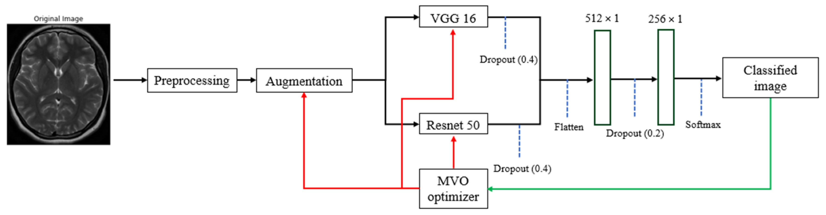
Figure 2.
An examples of applying the suggested preprocessing method. The original image is indicated to provide a baseline. The contour image illustrates the identified largest contour. The extreme points image marks the extreme points on the brain contour, demonstrating the cropping boundaries. The cropped image displays the isolated brain region, ready for input into the classification models.
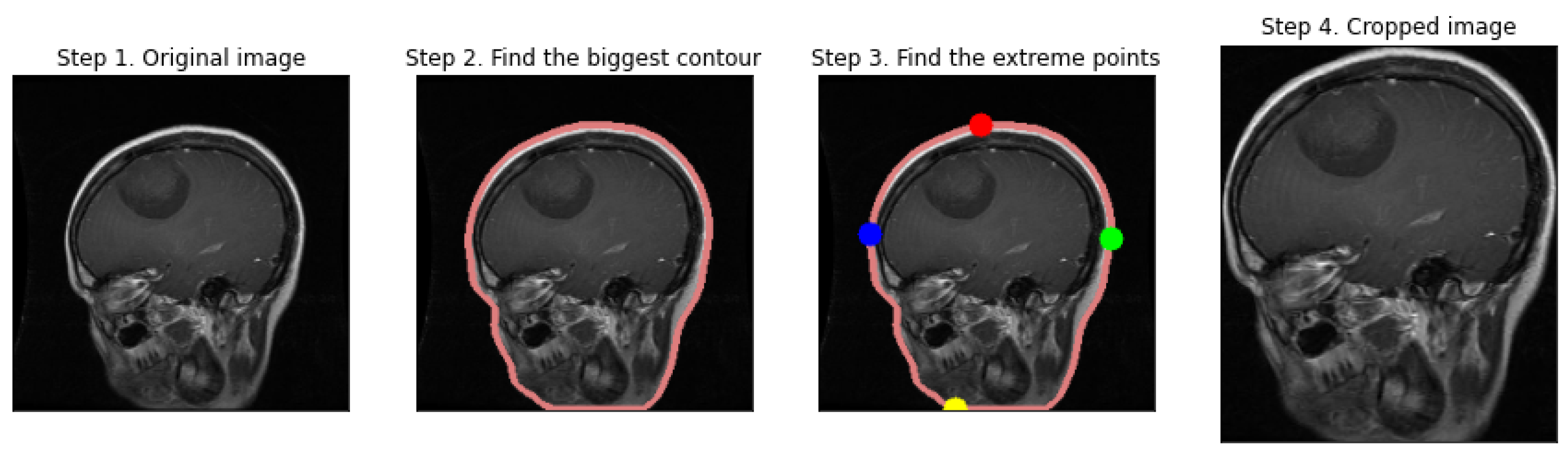
Figure 3.
The results of applying the augmentation methods to an image.
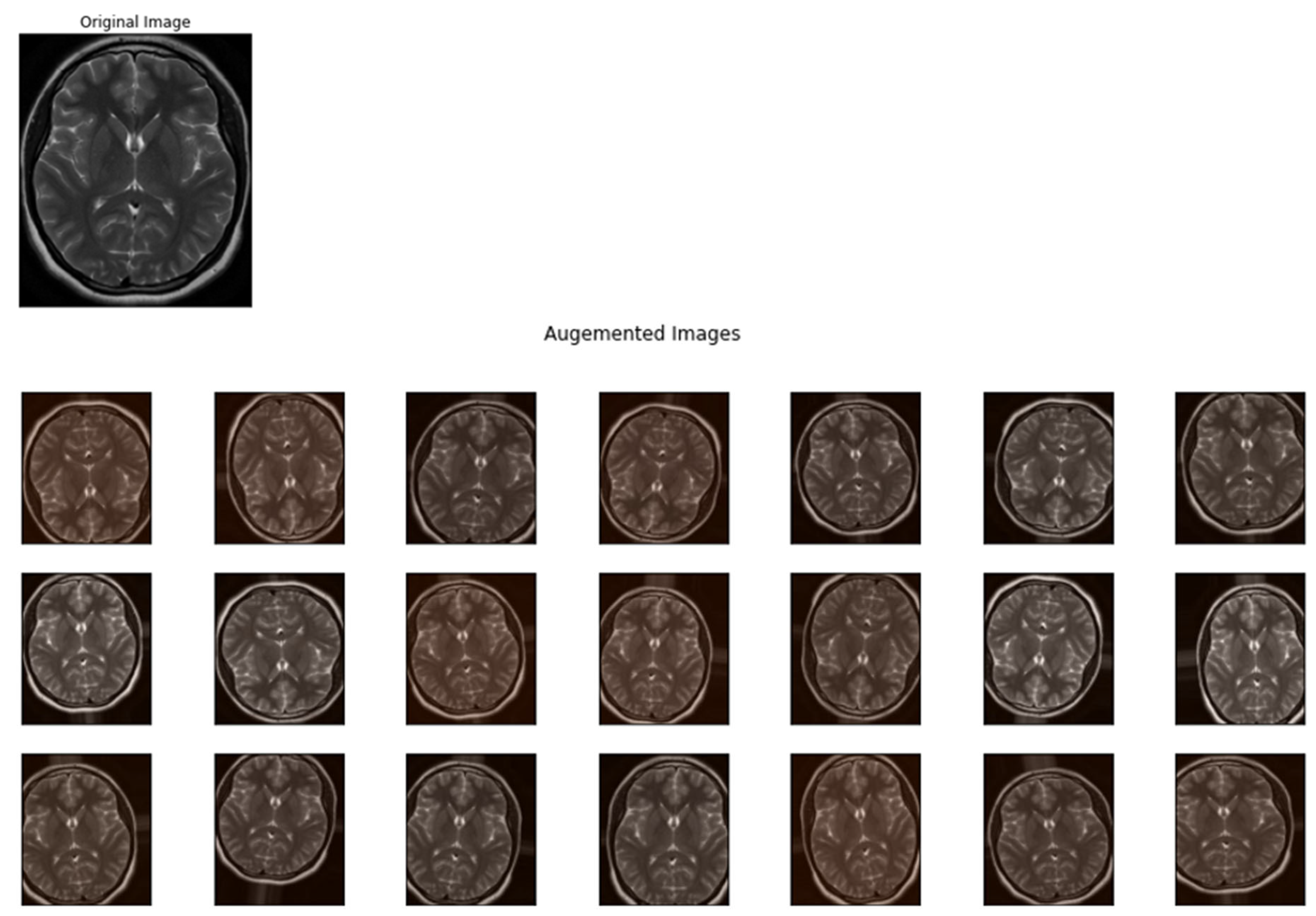
Figure 4.
Some images from the dataset samples.
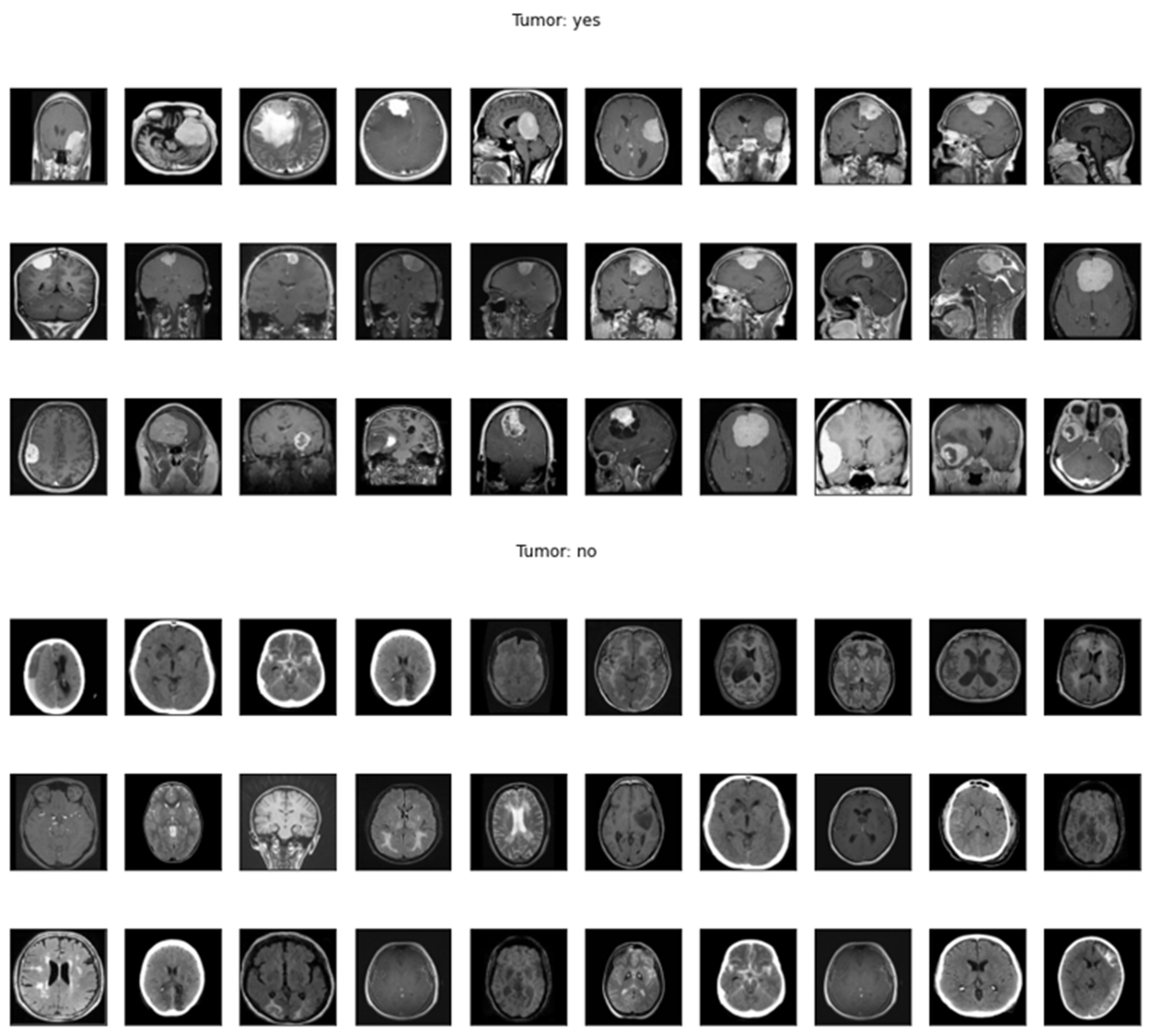
Figure 5.
Comparative performance analysis of DL models on MRI image classification.
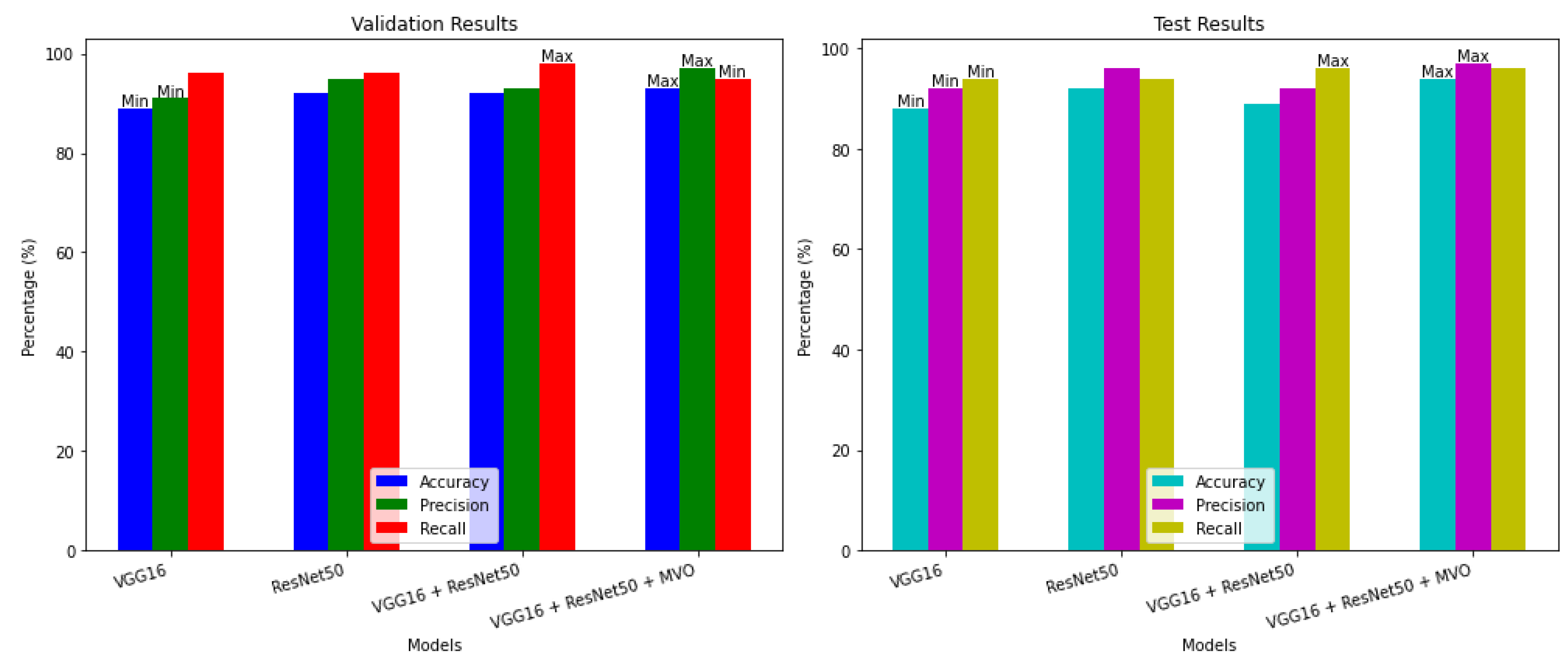
Figure 6.
The performance of the VGG16 model.
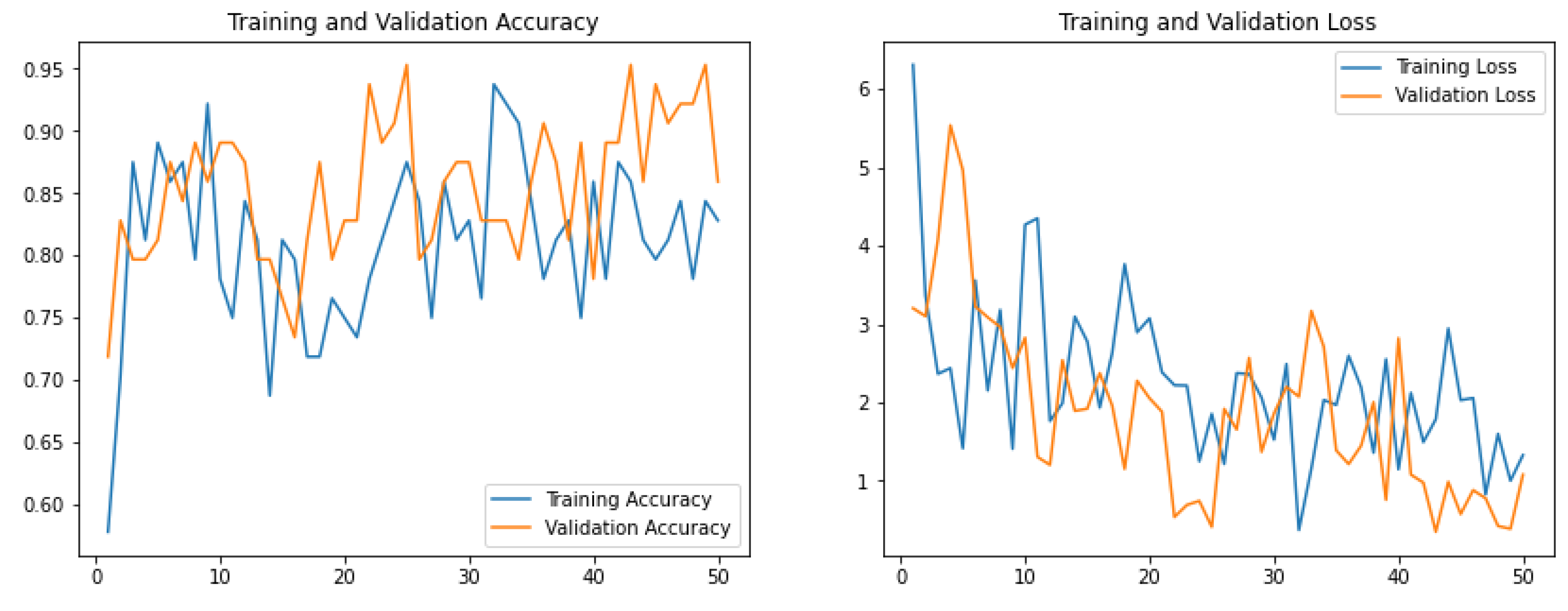
Figure 7.
The performance of the ResNet50 model.
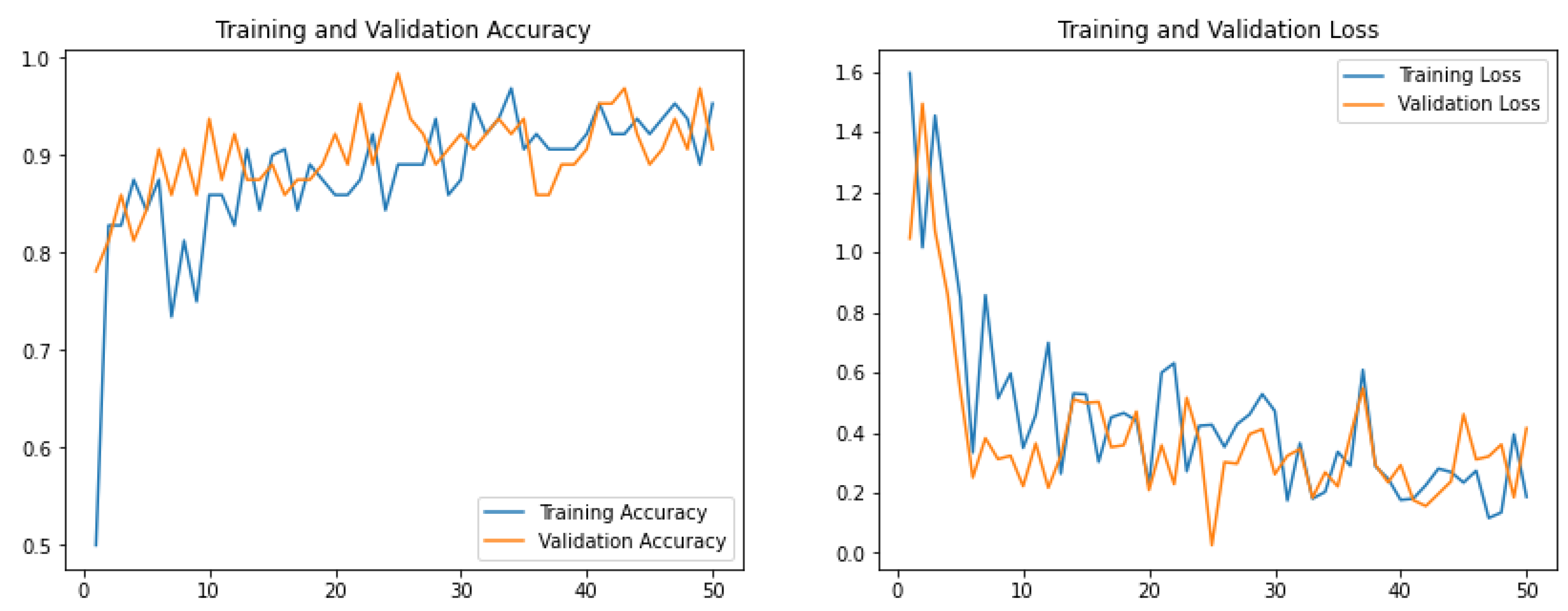
Figure 8.
The performance of our model without applying MVO optimizer. All layers in the ResNet50 and VGG16 were frozen.
Figure 8.
The performance of our model without applying MVO optimizer. All layers in the ResNet50 and VGG16 were frozen.
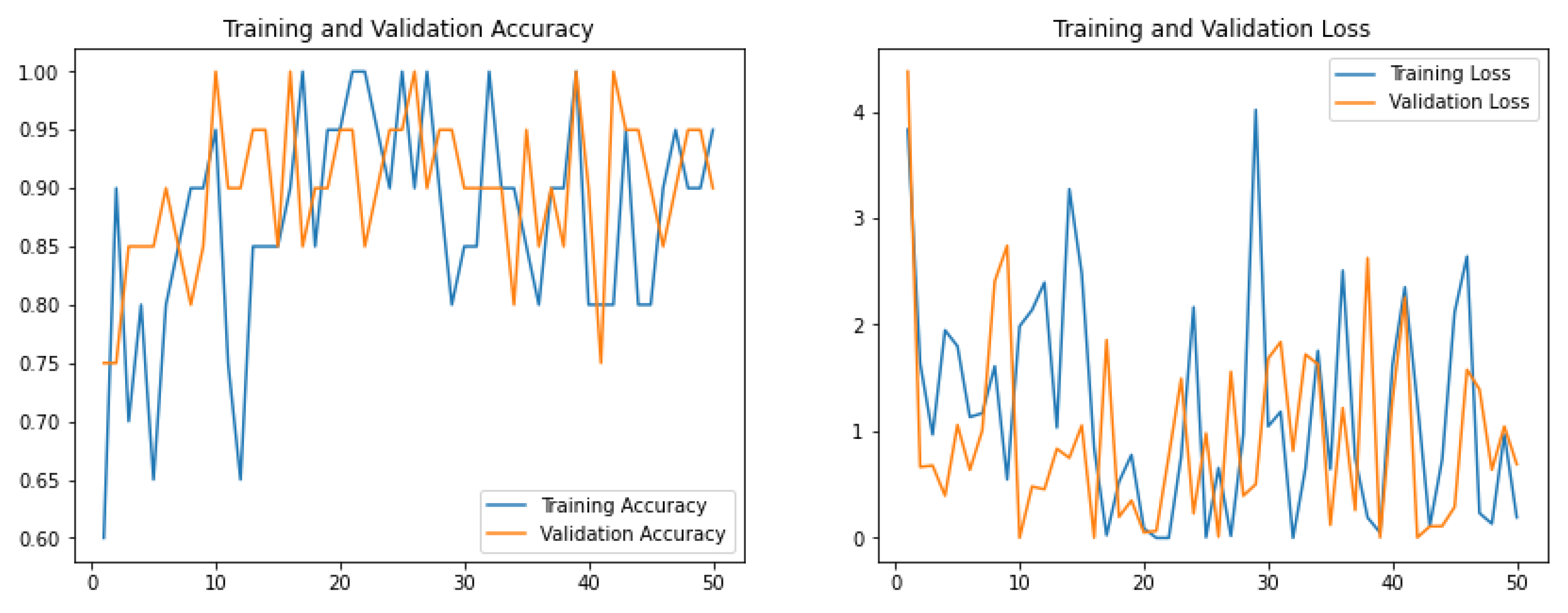
Figure 9.
The performance of our model using MVO optimizer.
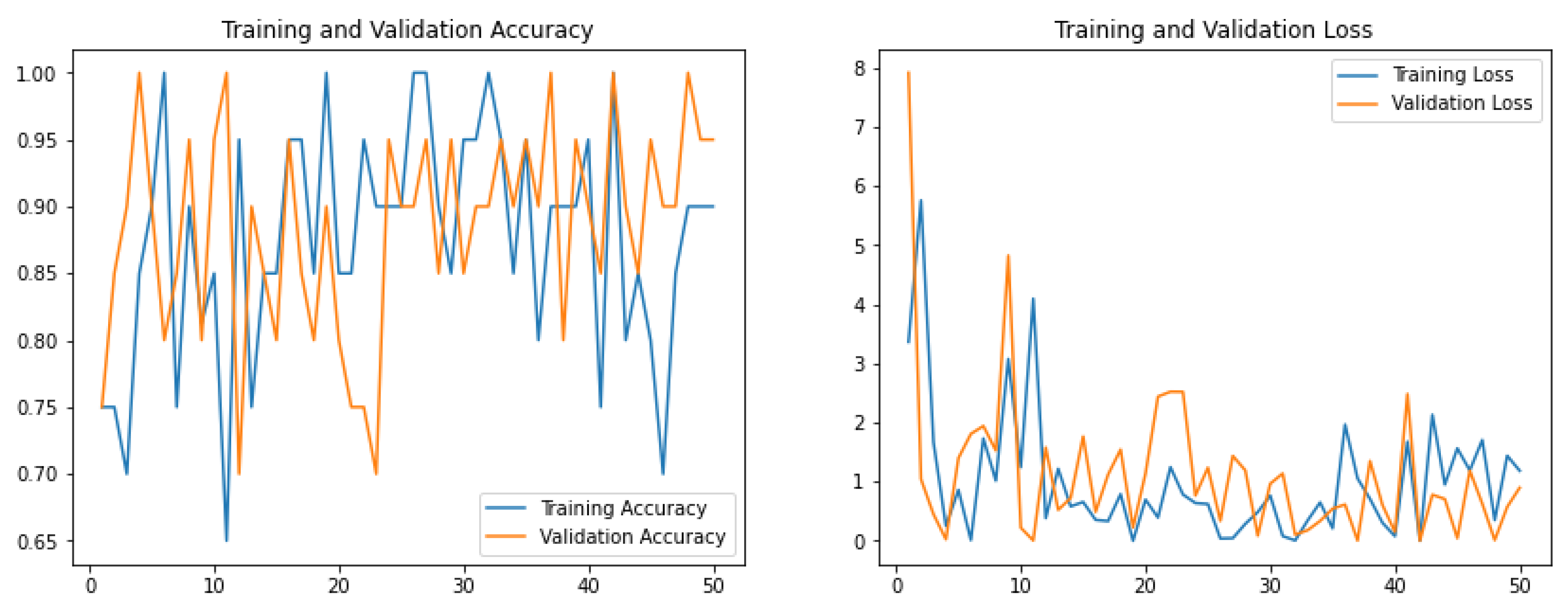
Figure 10.
The confusion matrix of the ResNet50 and VGG16 models.
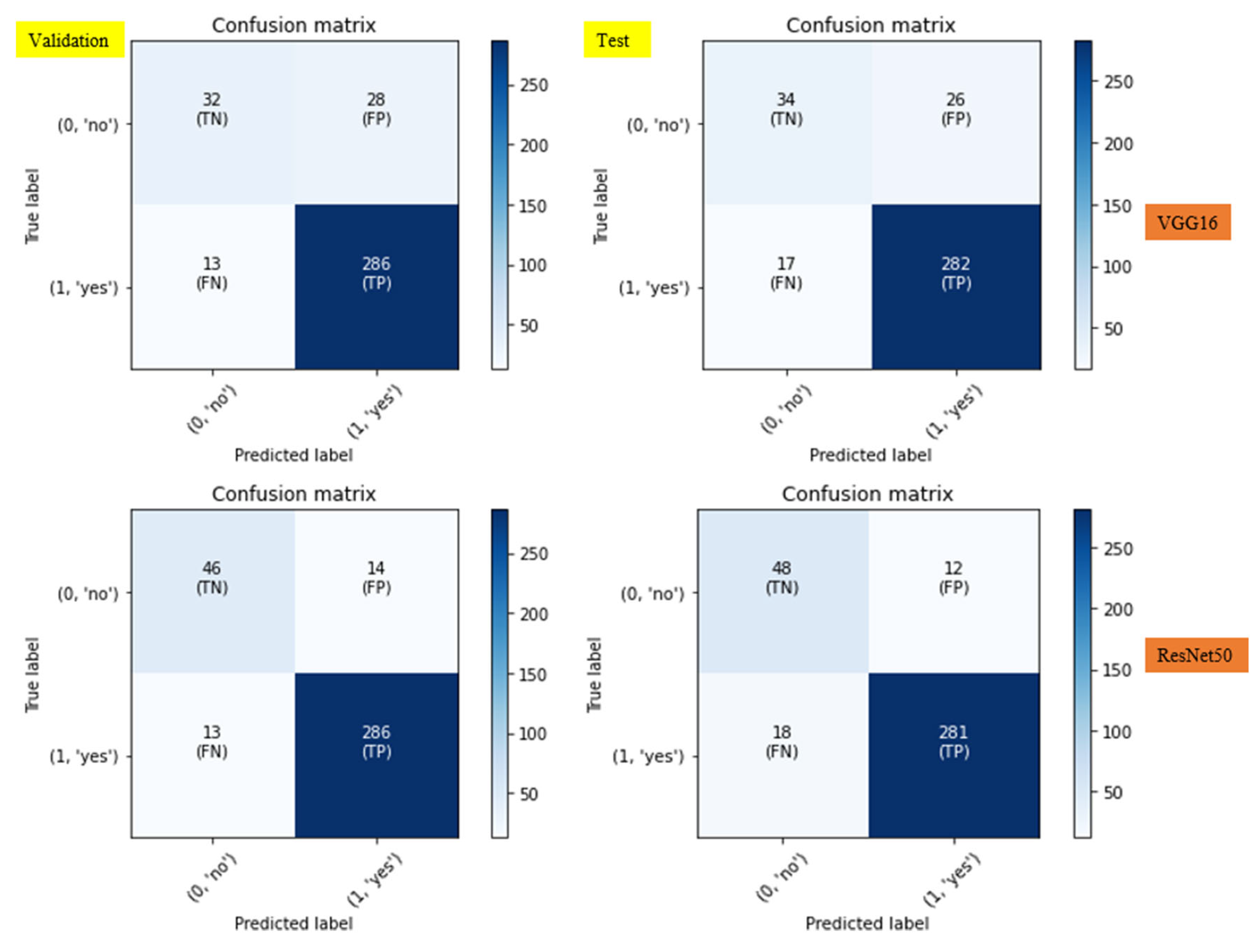
Figure 11.
The confusion matrix of our model.
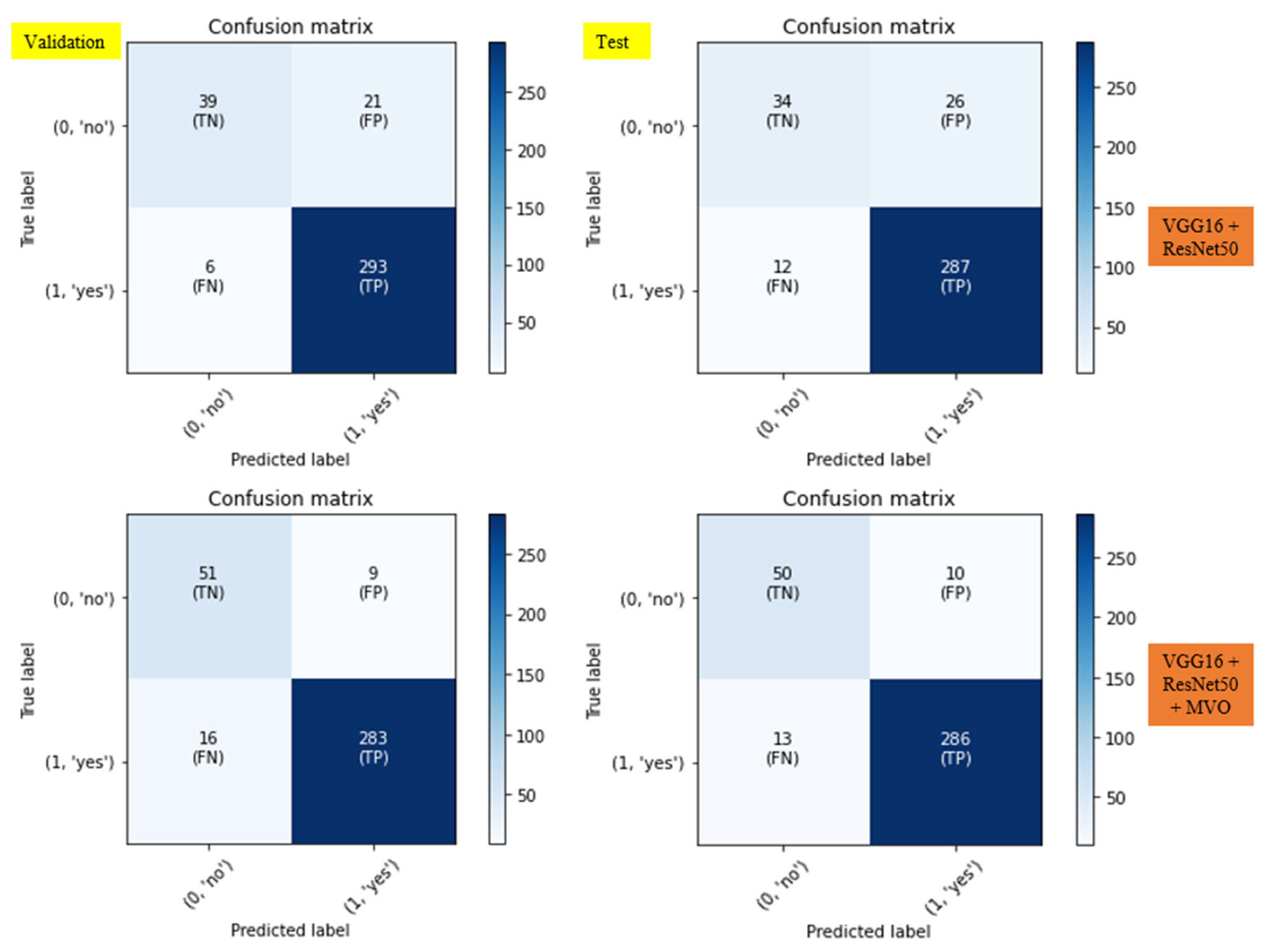
Figure 12.
The ROC curves of different models for evaluating the true positive rate against the false positive rate at various threshold settings.
Figure 12.
The ROC curves of different models for evaluating the true positive rate against the false positive rate at various threshold settings.
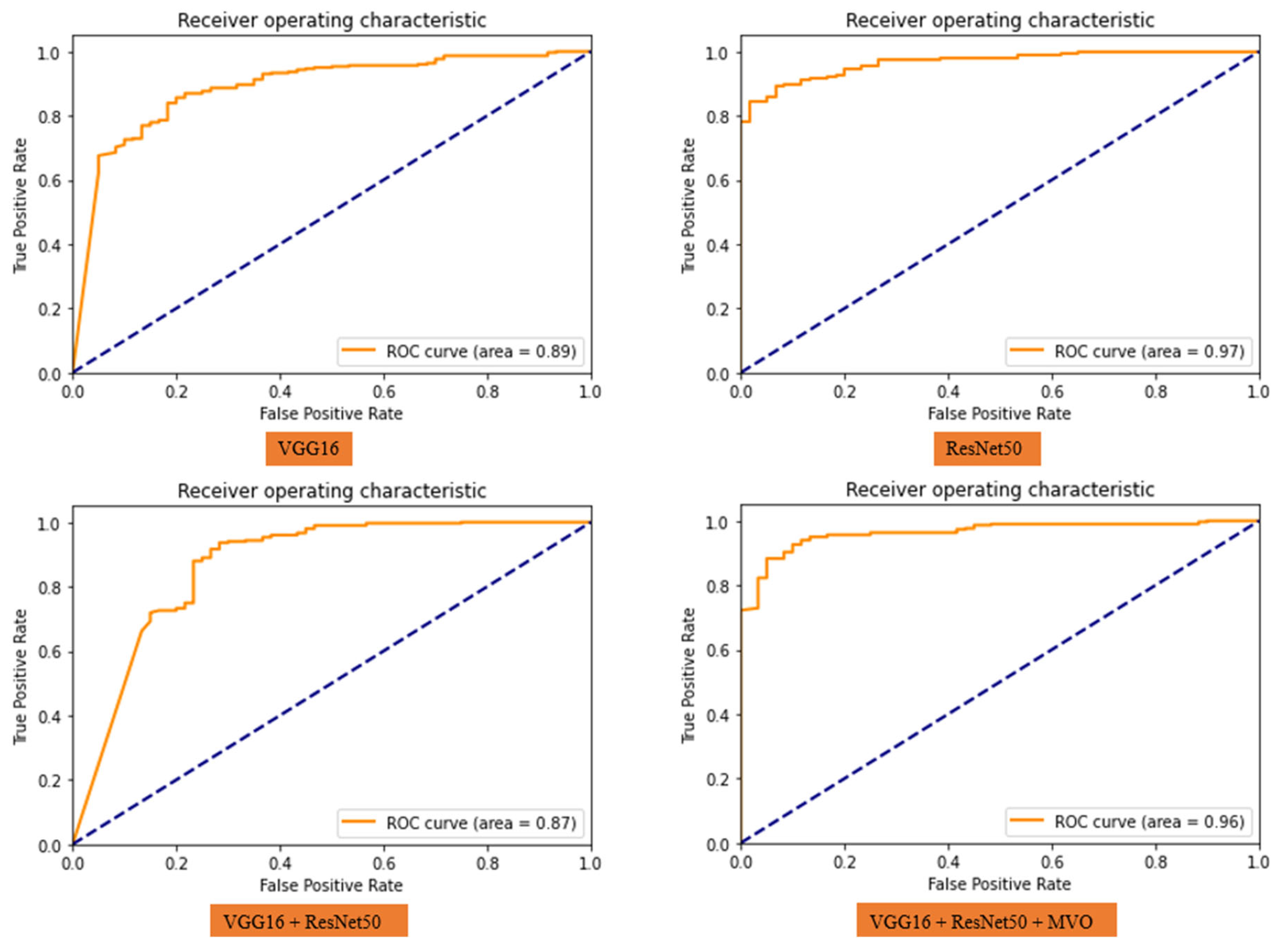
Figure 13.
Performance comparison of the suggested model with different optimization techniques.
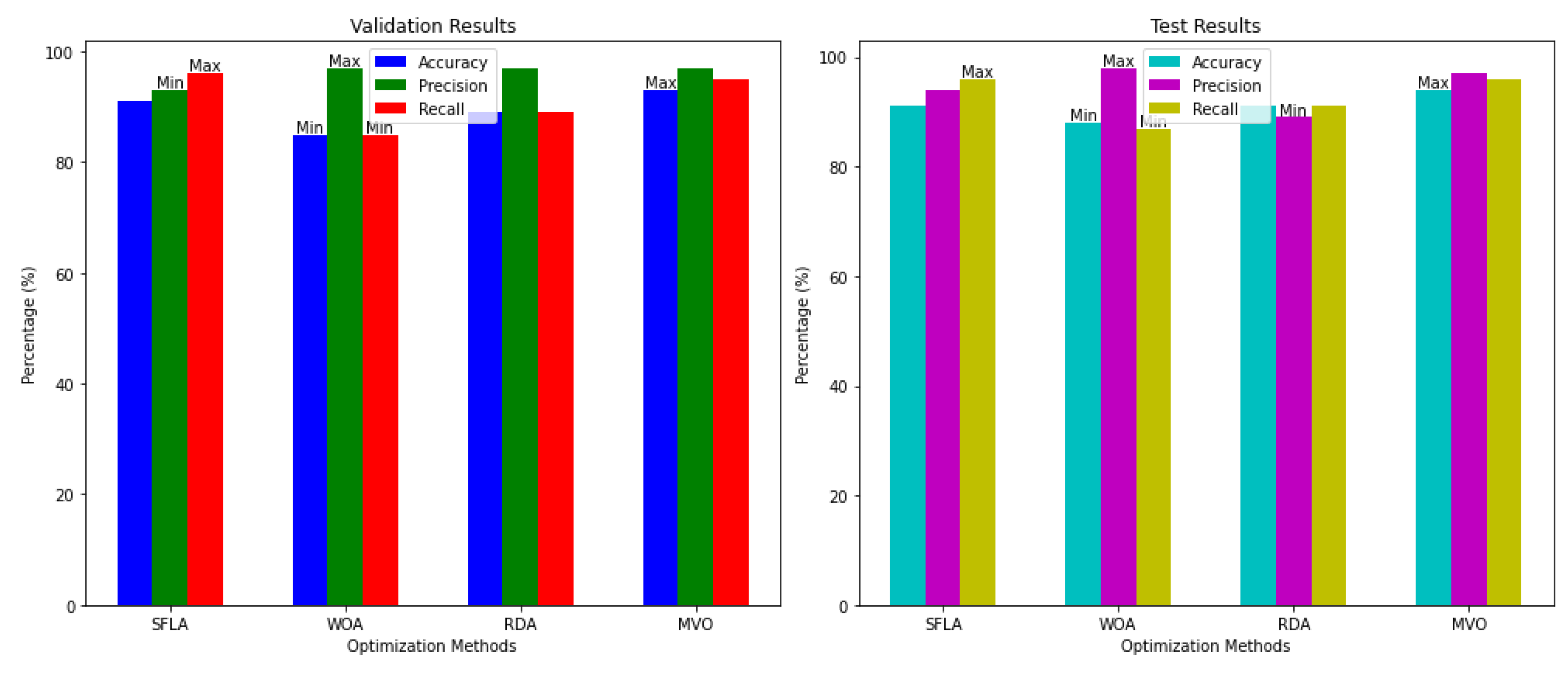

Table 1.
Specific parameters of the MVO algorithm that were employed for optimization purpose.
| Hyperparameters | Description | Best value |
|---|---|---|
| Universe Size | Number of solutions in the population | 30 |
| Wormhole Existence Probability (WEP) | Probability of wormholes' appearance | 0.6 |
| Travelling Distance Rate (TDR) | How far a wormhole can alter a solution | 0.4 |
| Max/Min WEP | Bounds the occurrence of wormholes | Max: 1.0, Min: 0.2 |
| Max/Min TDR | Limits the modification extent by the wormholes | Max: 1.0, Min: 0.4 |
Table 2.
Description of all data augmentation methods employed in our study. *Note: The 'Channel Shift' and 'Fill Mode' methods are not selected by the optimization approach for data augmentation.
Table 2.
Description of all data augmentation methods employed in our study. *Note: The 'Channel Shift' and 'Fill Mode' methods are not selected by the optimization approach for data augmentation.
| Index | Augmentation Method | Description | Used in Study | Suggested values by MVO optimizer |
|---|---|---|---|---|
| 1 | Rotation range | Random rotation within a specified range of degrees. | Yes | 10 |
| 2 | Width Shifting range | Random horizontal shift. | Yes | 0.1 |
| 3 | Height Shifting range | Random vertical shift. | Yes | 0.1 |
| 4 | Shear range | Random shearing. | Yes | 0.1 |
| 5 | Brightness range | Random brightness adjustments. | Yes | [0.5 1.5] |
| 6 | Horizontal Flip | Random horizontal flipping. | Yes | True |
| 7 | Vertical Flip | Random vertical flipping. | Yes | True |
| 8 | Zoom range | Random zooming into the images. | Yes | 0.1 |
| 9 | Channel Shift* | Random channel shifting. | No | - |
| 10 | Fill Mode* | Method for filling points outside the boundaries of the input. | No | - |
Table 3.
Quantitative outcomes of applying four models to the dataset.
| Data | Model | Accuracy (%) | Precision (%) | Recall(%) | Run results |
|---|---|---|---|---|---|
| Validation |
VGG16 |
89 | 91 | 96 |  |
| Test | 88 | 92 | 94 | ||
| Validation |
ResNet50 |
92 | 95 | 96 |  |
| Test | 92 | 96 | 94 | ||
| Validation |
VGG16 + ResNet50 |
92 | 93 | 98 |  |
| Test | 89 | 92 | 96 | ||
| Validation | VGG16 + ResNet50 + MVO | 93 | 97 | 95 | 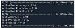 |
| Test | 94 | 97 | 96 |
Table 4.
The obtained results by applying different optimization approaches.
| Data | Model | Accuracy (%) | Precision (%) | Recall (%) |
|
|---|---|---|---|---|---|
| Validation | Our model + SFLA [66] | 91 | 93 | 96 | 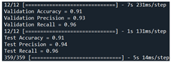 |
| Test | 91 | 94 | 96 | ||
| Validation | Our model + WOA [67] | 85 | 97 | 85 | 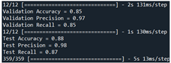 |
| Test | 88 | 98 | 87 | ||
| Validation | Our model + RDA [68] | 89 | 97 | 89 | 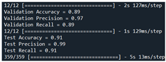 |
| Test | 91 | 89 | 91 | ||
| Validation | Our model + MVO [44] | 93 | 97 | 95 | 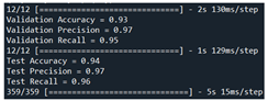 |
| Test | 94 | 97 | 96 |
Disclaimer/Publisher’s Note: The statements, opinions and data contained in all publications are solely those of the individual author(s) and contributor(s) and not of MDPI and/or the editor(s). MDPI and/or the editor(s) disclaim responsibility for any injury to people or property resulting from any ideas, methods, instructions or products referred to in the content. |
© 2024 by the authors. Licensee MDPI, Basel, Switzerland. This article is an open access article distributed under the terms and conditions of the Creative Commons Attribution (CC BY) license (http://creativecommons.org/licenses/by/4.0/).
Copyright: This open access article is published under a Creative Commons CC BY 4.0 license, which permit the free download, distribution, and reuse, provided that the author and preprint are cited in any reuse.


