Dynamic architecture adaptation for MRI brain tumor Detection using SECNNs

1. Introduction

1.1. Background

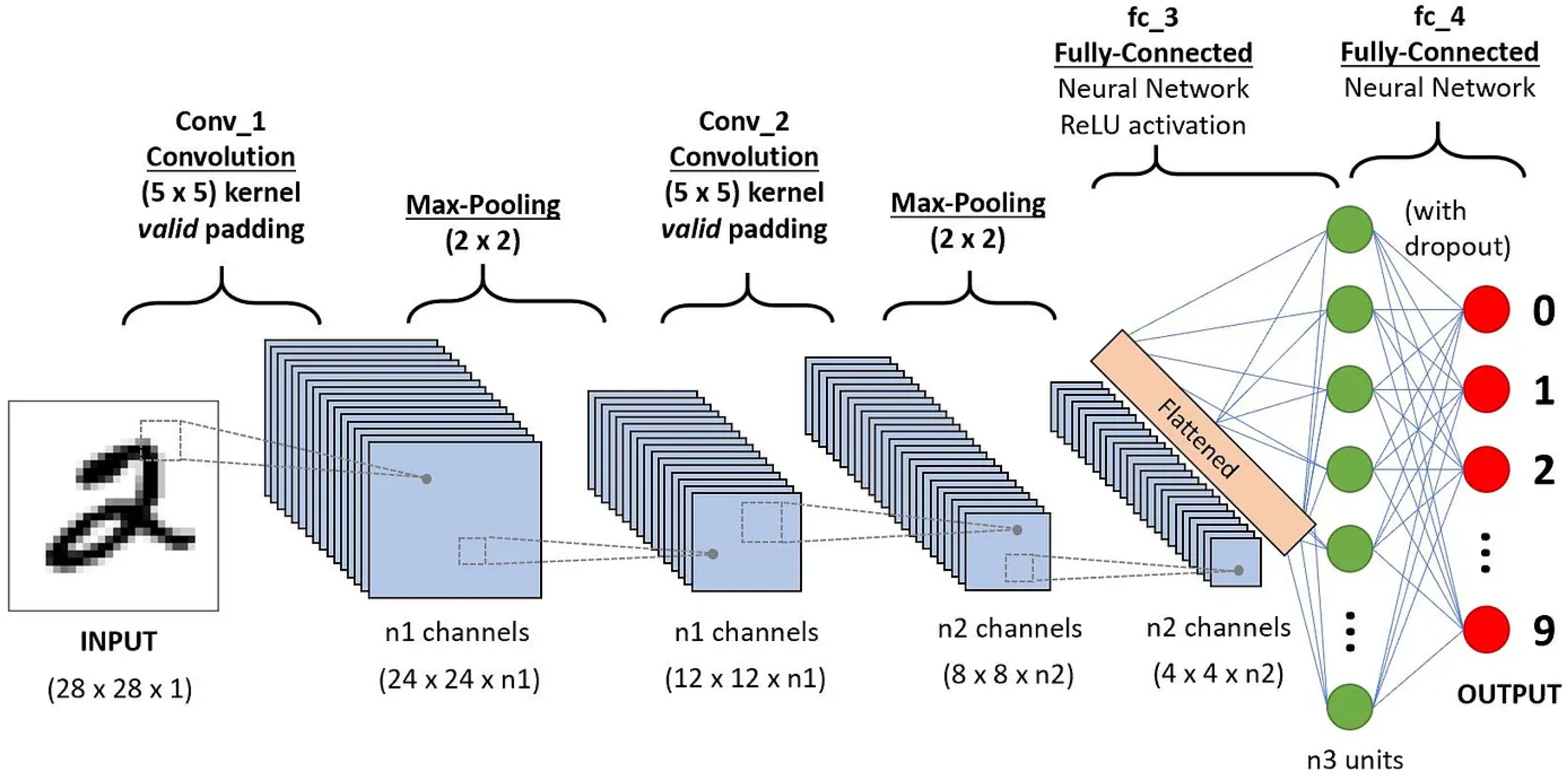
Convolutional Neural Networks (CNNs) have revolutionized the field of deep learning, particularly in processing grid-like data structures such as images. Their effectiveness in tasks like image classification, object detection, semantic segmentation, and image generation stems from their ability to efficiently learn spatial features. Convolutional layers, utilizing filters or kernels, capture local patterns and extract features from input images. A significant feature of convolutional layers is the shared weights implemented by kernels, which allow for efficient deep learning on images, as using only fully connected layers for such tasks would result in an unfathomable number of parameters. Pooling layers, such as max pooling and average pooling, reduce the spatial dimensions of these features, helping the network focus on the most significant aspects.

Figure 1. Convolutional Neural Network (CNN) architecture.

Figure 1. Convolutional Neural Network (CNN) architecture.

Despite their popularity, CNNs face challenges in computational efficiency and adaptability. Several architectures, such as MobileNet and EfficientNet, have been proposed to address these challenges. However, traditional CNNs with fixed architectures and parameter counts may not perform uniformly across different types of input data with varying levels of complexity. Neural Architecture Search (NAS) is a method for selecting optimal neural network architectures, responding to this challenge. NAS aims to identify the best model for a specific task under certain constraints. However, NAS is often resource-intensive, requiring the training of multiple candidate models to determine the optimal architecture. It is estimated that the carbon emissions produced when using NAS to train a transformer model can amount to five times the lifetime carbon emissions of an average car. This underscores the importance of finding suitable architectures for neural networks while also highlighting the limitations of current approaches in terms of static structure and susceptibility to over-parameterization.

Self-Expanding Neural Networks (SENN), introduced in 2021, offer a promising direction. Inspired by neurogenesis, SENN dynamically adds neurons and fully connected layers to the architecture during training, using a natural expansion score as a criterion to guide this process. This helps overcome the problem of over-parameterization. However, its application has been limited to multilayer perceptrons, with extensions to more practical architectures like CNNs identified as a future research prospect.

1.2. Importance of Detection Using ML

Identifying brain tumors from MRI images is a critical step in the diagnostic process. Accurate detection and differentiation of tumor types are essential for planning effective treatment strategies. With advancements in deep learning, particularly Convolutional Neural Networks (CNNs), machine learning systems have shown significant promise in achieving high accuracy. These systems can support radiologists by providing additional insights, thereby aiding in more informed and precise decision-making.

2. Objectives

The primary objective of this study is to develop a CNN-based model capable of accurately categorizing MRI images into four classes: glioma, meningioma, no tumor, and pituitary tumor. The secondary objective is to explore and document the various techniques and optimizations employed to enhance the model’s performance. Additionally, we aim to develop a Self-Expanding Convolutional Neural Network (SECNN), building on the concept of Self-Expanding Neural Networks (SENN) and applying it to modern vision tasks. This approach dynamically adjusts model complexity during training, thereby improving efficiency and adaptability. Unlike existing methods that often necessitate restarting training after modifications or rely on preset mechanisms for expansion, our approach leverages the natural expansion score for dynamic and optimal model growth.

2.1. Integrating CNN with SECNN

The integration process begins with a conventional Convolutional Neural Network (CNN) architecture, which can be represented by the following mathematical functions:

$$y=f(x;\theta )=\sigma (W_k\ast x+b)$$

(1)

where y is the output of the model, x is the input MRI images, $\theta$ represents the trainable parameters (weights and biases), * denotes the convolution operator, and $\sigma$ is the non-linear activation function.

To incorporate the self-expanding concept (SECNN), we introduce a mechanism to dynamically adjust the model complexity based on a natural expansion score, which can be represented by the following function:

$$E\left(t\right)=\sum _{i=1}^N\varphi \left(a_i\left(t\right)\right)$$

(2)

where $E\left(t\right)$ is the expansion score at time t, N is the number of neurons in the layer, and $\varphi \left(a_i\left(t\right)\right)$ is a function depending on the activation of neuron $a_i$ at time t.

Based on the expansion score $E\left(t\right)$, the model decides whether to add new layers or neurons:

$$\mathrm{If}E\left(t\right)>\tau ,\mathrm{then}\mathrm{add}\mathrm{new}\mathrm{layers}/\mathrm{neurons}$$

(3)

where $\tau$ is a predefined threshold.

Through this mechanism, the network structure is adjusted during training to continuously improve performance without the need to restart training or rely on static architectures. This research represents a significant step forward in creating adaptable and efficient CNN models for a variety of vision-related tasks.

3. Dataset Description

3.1. Dataset Overview

The dataset used in this study is a combination of multiple sources, providing a total of 7023 MRI images divided into four classes:

• Glioma: Cancerous tumors in glial cells.
• Meningioma: Non-cancerous tumors originating from the meninges.
• No Tumor: Normal brain scans without detectable tumors.
• Pituitary: Tumors affecting the pituitary gland, which can be either cancerous or non-cancerous.

3.2. Data Preprocessing

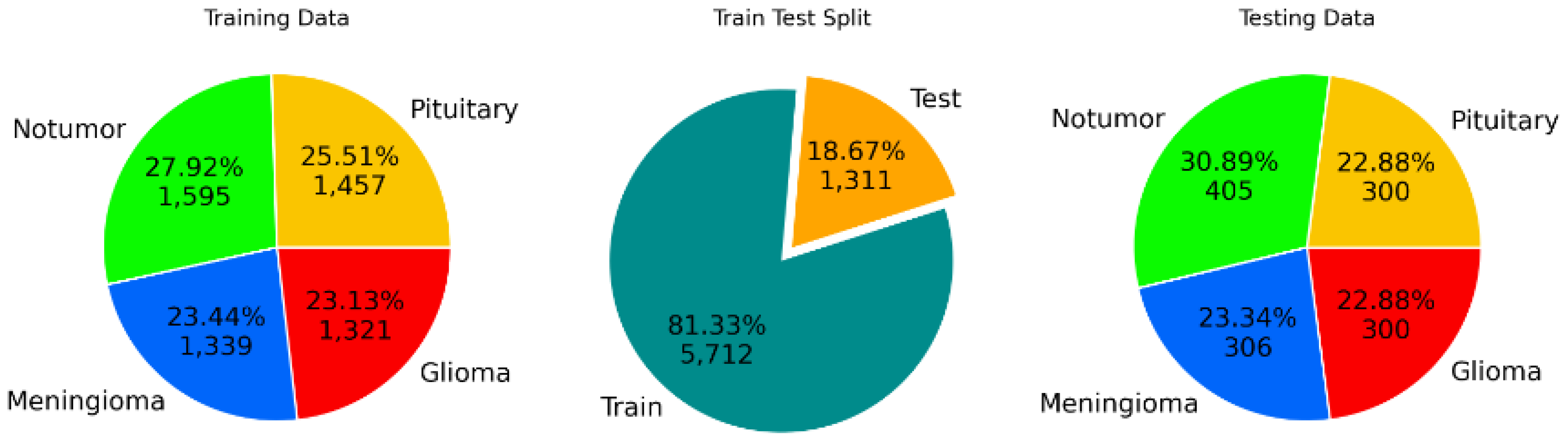
Data preprocessing includes resizing images to a consistent dimension of (150, 150, 3), normalizing pixel values, and applying data augmentation techniques to enhance dataset diversity. The training set consists of 5712 images with the following distribution: 1457 pituitary, 1595 no tumor, 1339 meningioma, and 1321 glioma. The testing set consists of 1311 images with the following distribution: 300 pituitary, 405 no tumor, 306 meningioma, and 300 glioma.

Figure 2. Data sampling process for MRI images.

Figure 2. Data sampling process for MRI images.

4. Methodology

4.1. Neural Networks: A Detailed Overview

4.1.1. Neural Networks

A neural network is a computational model inspired by the way biological neural networks in the human brain process information. It consists of interconnected nodes, or neurons, organized into layers. The primary components of a neural network are:

• Input Layer: This layer receives the input data and passes it to subsequent layers.
• Hidden Layers: These intermediate layers process the inputs received from the input layer through various transformations and activations. They play a crucial role in feature extraction and pattern learning.
• Output Layer: The final layer produces the network’s output based on the processed information from the hidden layers.

Each connection between neurons has an associated weight, which adjusts as the network learns. The process of adjusting weights based on the error of the output is called training.

4.1.2. Mathematical Foundation of Neural Networks

The basic operation of a neural network involves a series of dot products followed by activation functions. For a single neuron, the operation can be described mathematically as follows:

$$z=\sum _{i=1}^n{w}_i{x}_i+b$$

where z is the weighted sum of the inputs $x_i$ with weights $w_i$ and bias b. The neuron output y is then obtained by applying an activation function $\sigma$:

$$y=\sigma \left(z\right)$$

Common activation functions include:

• Sigmoid: $\sigma \left(z\right)=\frac{1}{1+e^{-z}}$
• ReLU (Rectified Linear Unit): $\sigma \left(z\right)=max(0,z)$
• Tanh: $\sigma \left(z\right)=tanh\left(z\right)$

4.1.3. Forward and Backward Propagation

Neural networks learn through a process called forward and backward propagation:

• Forward Propagation: The input data is passed through the network layer by layer to obtain the final output. Each neuron calculates its output using the weighted sum of its inputs and the activation function.
• Backward Propagation: The error between the predicted output and the actual output is calculated. This error is then propagated backward through the network, adjusting the weights using the gradient descent optimization algorithm. The weight update rule for gradient descent is:

  $$w_{ij}=w_{ij}-\eta \frac{\partial L}{\partial w_{ij}}$$

  where $\eta$ is the learning rate, L is the loss function, and $\frac{\partial L}{\partial w_{ij}}$ is the gradient of the loss function with respect to the weight $w_{ij}$.

4.2. Integrating CNN with SECNN

The integration process begins with a conventional Convolutional Neural Network (CNN) architecture, which can be represented by the following mathematical functions:

$$y=f(x;\theta )=\sigma (W_k\ast x+b)$$

(4)

where y is the output of the model, x is the input MRI images, $\theta$ represents the trainable parameters (weights and biases), * denotes the convolution operator, and $\sigma$ is the non-linear activation function.

To incorporate the self-expanding concept (SECNN), we introduce a mechanism to dynamically adjust the model complexity based on a natural expansion score, which can be represented by the following function:

$$E\left(t\right)=\sum _{i=1}^N\varphi \left(a_i\left(t\right)\right)$$

(5)

where $E\left(t\right)$ is the expansion score at time t, N is the number of neurons in the layer, and $\varphi \left(a_i\left(t\right)\right)$ is a function depending on the activation of neuron $a_i$ at time t.

Based on the expansion score $E\left(t\right)$, the model decides whether to add new layers or neurons:

$$\mathrm{If}E\left(t\right)>\tau ,\mathrm{then}\mathrm{add}\mathrm{new}\mathrm{layers}/\mathrm{neurons}$$

(6)

where $\tau$ is a predefined threshold.

Through this mechanism, the network structure is adjusted during training to continuously improve performance without the need to restart training or rely on static architectures. This approach allows the model to dynamically grow and adapt its complexity based on the data, thereby improving both efficiency and adaptability.

4.2.1. Implementation of SECNN in Practice

In practice, implementing a Self-Expanding Convolutional Neural Network (SECNN) involves monitoring the performance of the network during training and calculating the natural expansion score at regular intervals. When the score exceeds a certain threshold, additional neurons or layers are integrated into the network. This process helps in maintaining a balance between model complexity and computational efficiency.

Moreover, to ensure the stability of the network during expansion, a gradual integration approach is employed. New neurons or layers are initially introduced with smaller weights, which are then adjusted over subsequent training iterations. This gradual integration minimizes disruption to the network’s learning process and allows for a smoother adaptation to the increased complexity.

Integrating CNN with SECNN presents a novel approach to creating adaptable neural networks that can dynamically adjust their complexity based on the data, leading to enhanced performance and computational efficiency across a variety of vision-related tasks.

4.2.2. Loss Function

The loss function measures the discrepancy between the predicted output and the actual output, serving as a critical component in training neural networks. Common loss functions include:

• Mean Squared Error (MSE): Used primarily for regression tasks, it calculates the average squared difference between the actual and predicted values.

  $$L=\frac{1}{n}\sum _{i=1}^n{(y_i-{\widehat{y}}_i)}^2$$

  where $y_i$ represents the actual values, ${\widehat{y}}_i$ represents the predicted values, and n is the number of samples.
• Cross-Entropy Loss: Commonly used for classification tasks, it measures the performance of a classification model whose output is a probability value between 0 and 1.

  $$L=-\frac{1}{n}\sum _{i=1}^n[y_{i}log\left({\widehat{y}}_i\right)+(1-y_i)log(1-{\widehat{y}}_i)]$$

  where $y_i$ represents the actual class labels and ${\widehat{y}}_i$ represents the predicted probabilities.

4.2.3. Optimization Algorithms

Optimization algorithms are employed to adjust the weights of the neural network in order to minimize the loss function. Common optimization algorithms include:

• Stochastic Gradient Descent (SGD): An iterative method that updates the weights using a single or a small batch of training examples at each iteration, defined by the rule:

  $$w=w-\eta \nabla L\left(w\right)$$

  where $\eta$ is the learning rate and $\nabla L\left(w\right)$ is the gradient of the loss function with respect to the weights.
• Adam: Combines the advantages of two other extensions of stochastic gradient descent, namely Adaptive Gradient Algorithm (AdaGrad) and Root Mean Square Propagation (RMSProp). It computes adaptive learning rates for each parameter by maintaining a running average of both the gradients and their second moments.

  $$w=w-\eta \frac{m_t}{\sqrt{v_t}+ϵ}$$

  where $m_t$ is the first moment estimate, $v_t$ is the second moment estimate, and $ϵ$ is a small constant for numerical stability.

4.3. Convolutional Neural Networks (CNNs)

Convolutional Neural Networks (CNNs) are specialized neural networks designed for processing data with a grid-like topology, such as images. They consist of convolutional layers, pooling layers, and fully connected layers, each serving a distinct function in the feature extraction and learning process.

4.3.1. Convolutional Layer

The convolutional layer applies a set of learnable filters (kernels) to the input image. This operation captures local patterns and features from the input data. The mathematical operation for a single convolutional layer can be expressed as:

$$O_{i,j,k}=\sum _{m=1}^M\sum _{n=1}^N\sum _{c=1}^C{I}_{i+m,j+n,c}·K_{m,n,c,k}+b_k$$

where I is the input image, K is the kernel, $b_k$ is the bias term, and O is the output feature map. Here, i and j denote the spatial dimensions, c is the input channel, and k is the output channel.

Figure 3. Structure of the CNN model used for MRI classification.

Figure 3. Structure of the CNN model used for MRI classification.

Figure 4. Convolutional layer in a CNN.

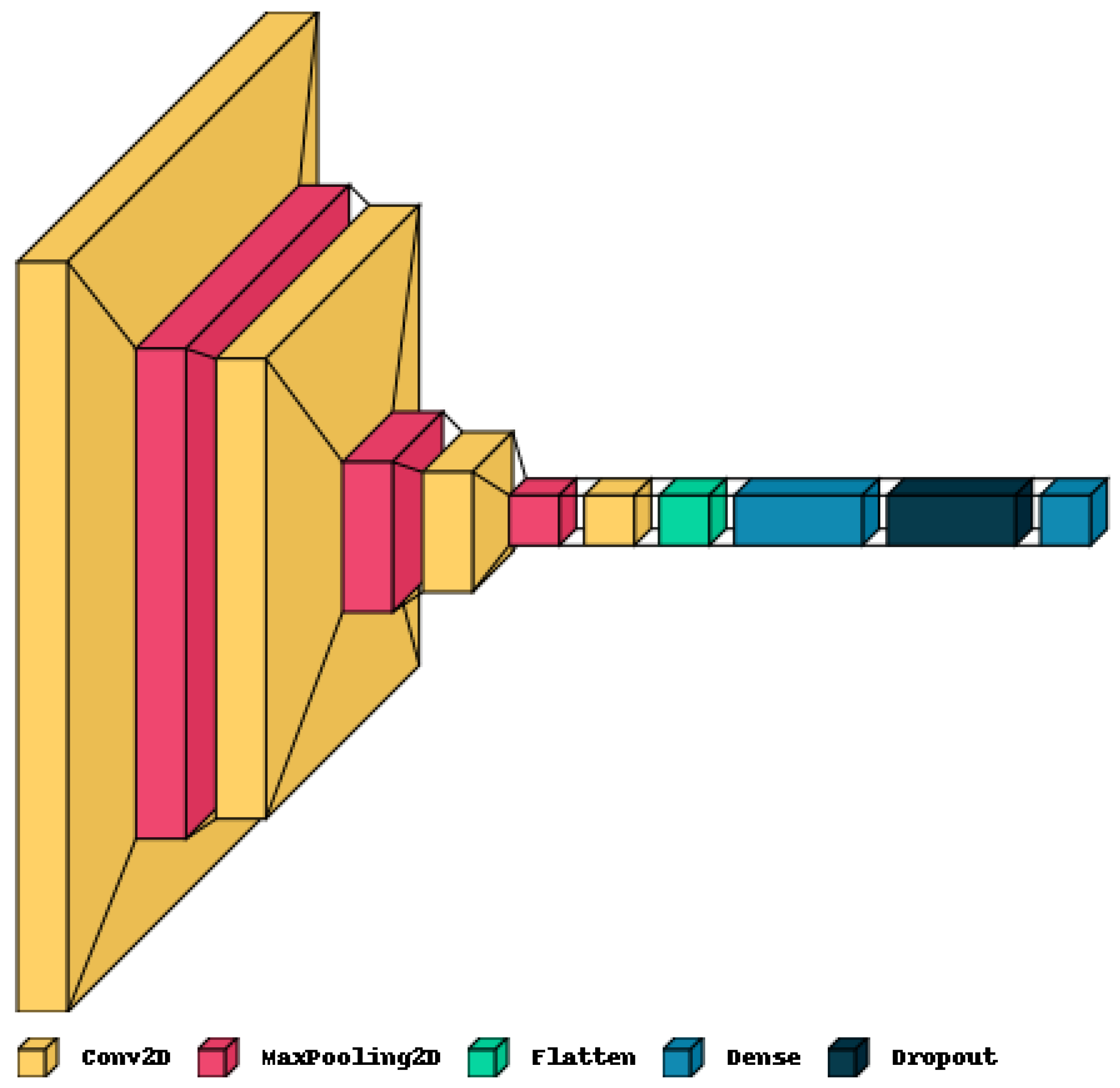
Figure 4. Convolutional layer in a CNN.

4.3.2. Pooling Layer

The pooling layer reduces the spatial dimensions of the input, thereby decreasing the computational load and helping to extract dominant features. The most common type is max pooling, which selects the maximum value within a defined window. The operation is defined as:

$$P_{i,j,k}=max\left(O_{i+m,j+n,k}\right)$$

where P is the pooled output, and the indices m and n define the window size for the pooling operation.

Figure 5. Max pooling operation in a CNN.

Figure 5. Max pooling operation in a CNN.

4.3.3. Fully Connected Layer

In fully connected layers, every neuron is connected to every neuron in the previous layer. The operation is given by:

$$F_i=\sigma \left(\sum _{j=1}^N{W}_{ij}{x}_j+b_i\right)$$

where $\sigma$ is the activation function (e.g., ReLU), W is the weight matrix, x is the input vector, and b is the bias term.

4.4. Data Augmentation

Data augmentation techniques, such as rotation, brightness adjustment, width and height shifts, shear transformation, and horizontal flipping, are applied to the training images to prevent overfitting and improve generalization.

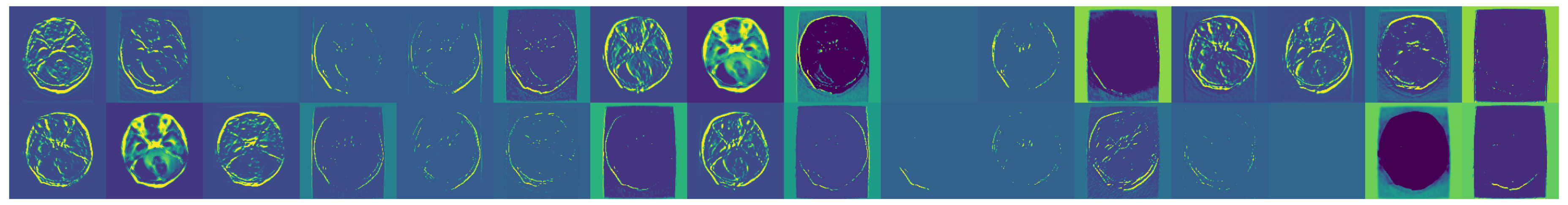
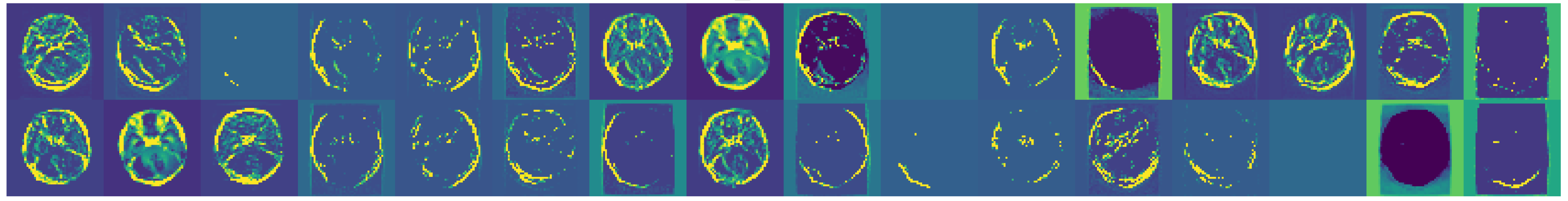
Figure 6. Examples of augmented images showcasing the diversity introduced.

Figure 6. Examples of augmented images showcasing the diversity introduced.

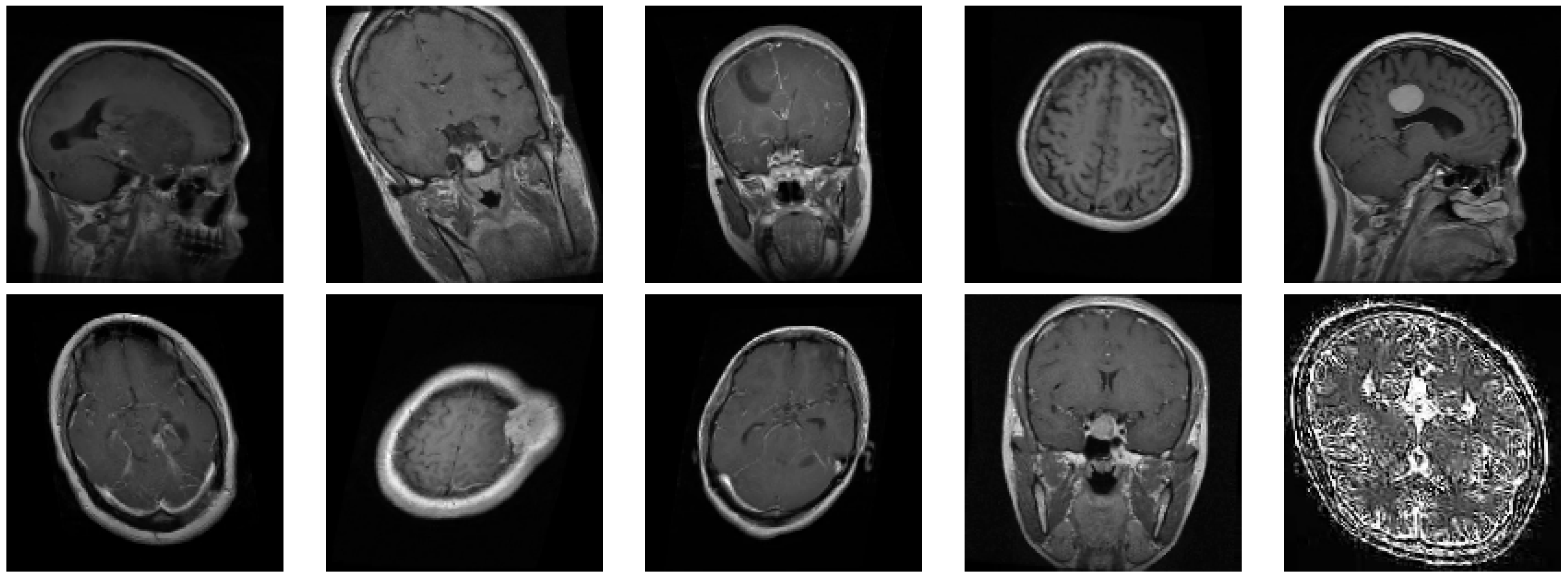
Figure 7. Further examples showcasing the diversity of transformations.

Figure 7. Further examples showcasing the diversity of transformations.

4.5. Model Optimization

The Adam optimizer is employed with fine-tuned parameters to achieve optimal performance. Techniques such as early stopping and learning rate reduction are implemented to enhance training efficiency and prevent overfitting. Early stopping monitors the model’s performance on a validation set and halts training when performance degrades, while learning rate reduction decreases the learning rate when the validation performance plateaus, allowing for finer adjustments during training.

4.6. Performance Metrics

To evaluate the model’s performance, we utilize several metrics, including accuracy, precision, recall, F1-score, and confusion matrix analysis:

• Precision: Measures the ability of the model to correctly identify positive instances for each class among all instances predicted as positive.

  $${\mathrm{Precision}}_c=\frac{T{P}_c}{T{P}_c+F{P}_c}$$

  where $T{P}_c$ denotes the true positives and $F{P}_c$ denotes the false positives for class c.
• Recall (Sensitivity or True Positive Rate): Calculates the ability of the model to correctly identify positive instances for each class among all actual positive instances.

  $${\mathrm{Recall}}_c=\frac{T{P}_c}{T{P}_c+F{N}_c}$$

  where $T{P}_c$ denotes the true positives and $F{N}_c$ denotes the false negatives for class c.
• F1-Score: The harmonic mean of precision and recall. It provides a balanced measure that combines both metrics for each class.

  $${\mathrm{F}1-\mathrm{Score}}_c=\frac{2·({\mathrm{Precision}}_c·{\mathrm{Recall}}_c)}{{\mathrm{Precision}}_c+{\mathrm{Recall}}_c}$$
• Accuracy: Measures the overall correctness of the model’s predictions across all classes.

  $$\mathrm{Accuracy}=\frac{{\sum }_{i=1}^{N}T{P}_i}{{\sum }_{i=1}^N(T{P}_i+F{P}_i+F{N}_i)}$$

  where N is the number of classes, $T{P}_i$ is the true positives, $F{P}_i$ is the false positives, and $F{N}_i$ is the false negatives for class i.

4.7. Self-Expanding Convolutional Neural Networks (SECNNs)

Self-Expanding Convolutional Neural Networks (SECNNs) are an advanced variant of CNNs that dynamically adjust their architecture during training. This approach addresses the issues of over-parameterization and computational inefficiency by expanding the network only when necessary.

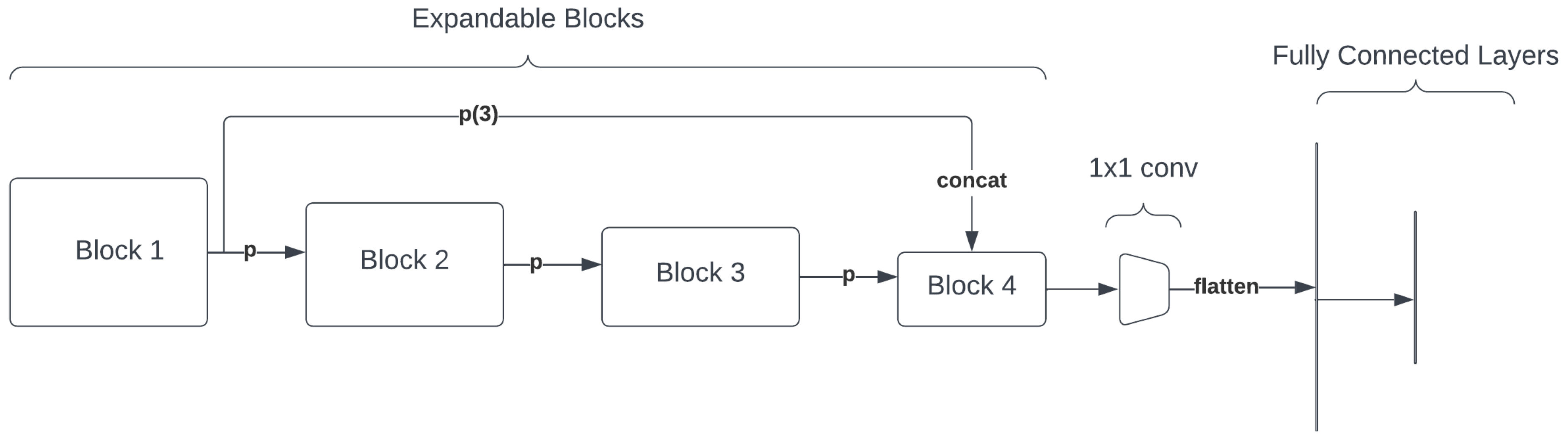
Figure 8. Self-Expanding Convolutional Neural Network (SECNN) architecture.

Figure 8. Self-Expanding Convolutional Neural Network (SECNN) architecture.

4.7.1. Natural Expansion Score

The natural expansion score is a crucial metric used to determine when and how to expand the network. It is calculated as follows:

$$\eta =g^T{F}^{-1}g$$

where F is the Fisher Information Matrix (FIM), and g is the gradient. For computational efficiency, the empirical Fisher approximation is used:

$$F=\frac{1}{N}\sum _{i=1}^N{\nabla }_{\theta }L(\theta ;x_i){\nabla }_{\theta }L{(\theta ;x_i)}^T$$

where $\theta$ represents the model parameters, L is the loss function, and $x_i$ are the input data samples.

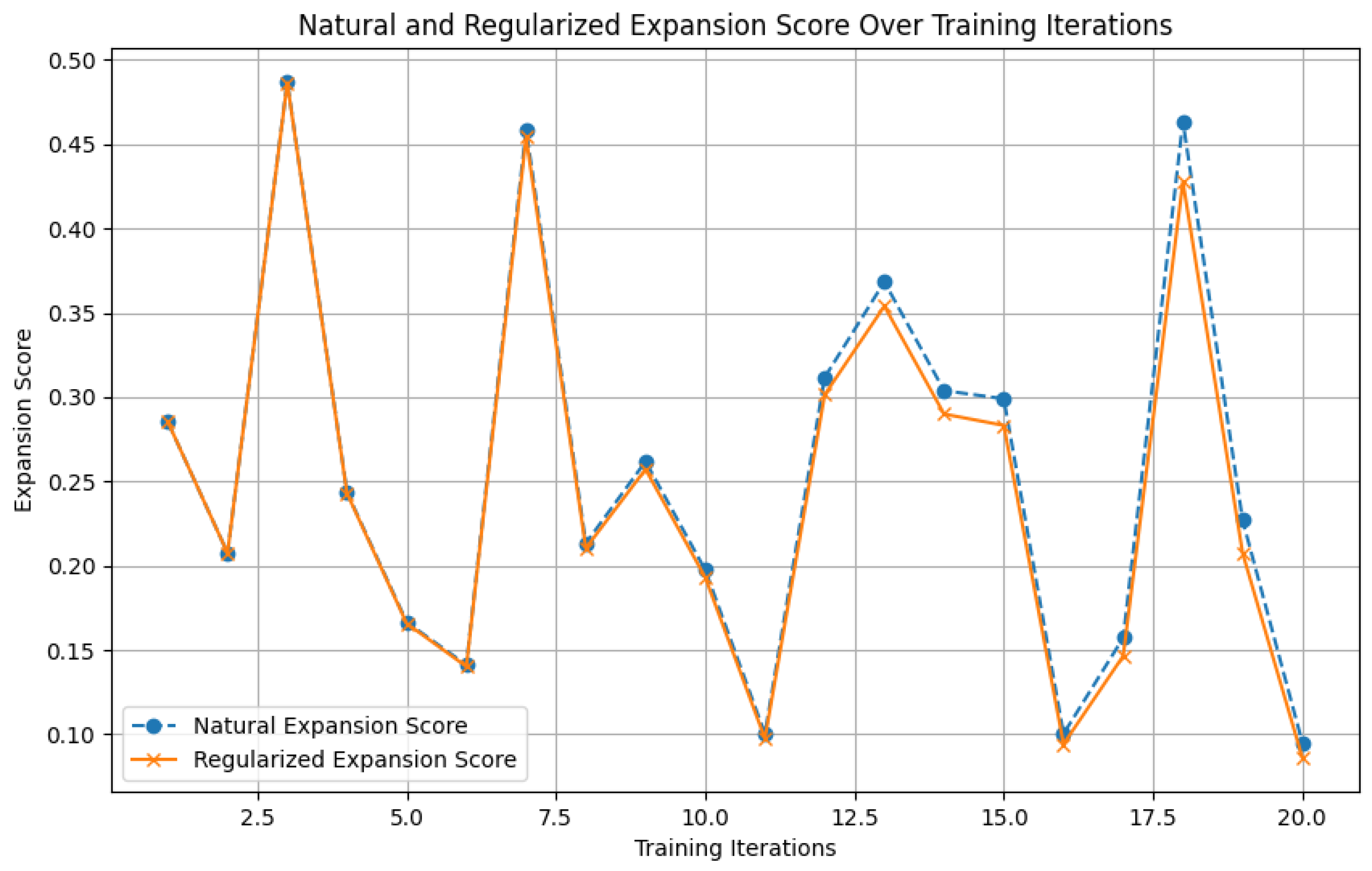
To prevent over-expansion, a regularization term is added to the natural expansion score:

$${\eta }_{\mathrm{regularized}}=\eta \times exp(-{\lambda }_n\times \Delta p^2)$$

where ${\lambda }_n$ is the regularization coefficient, and $\Delta p^2$ is the increase in parameters. This regularization term ensures that the network only expands when the benefits outweigh the cost of increased complexity.

Figure 9. Illustration of the natural expansion score calculation and regularization.

Figure 9. Illustration of the natural expansion score calculation and regularization.

4.7.2. Model Expansion Strategy

The model dynamically expands by adding layers or increasing the number of channels based on the natural expansion score. This strategy ensures optimal model complexity while maintaining computational efficiency. Specifically, during training, the natural expansion score guides the addition of convolutional layers or increases the number of filters within layers. This dynamic adjustment helps to match the model complexity with the data complexity, preventing overfitting and underfitting.

Mathematically, the expansion criterion can be expressed as:

$$\eta =\frac{1}{N}\sum _{i=1}^N{\left({\nabla }_{\theta }L(\theta ;x_i)\right)}^T\left(F^{-1}{\nabla }_{\theta }L(\theta ;x_i)\right)$$

where $\eta$ represents the expansion score, ${\nabla }_{\theta }L(\theta ;x_i)$ is the gradient of the loss function with respect to the parameters, and F is the Fisher Information Matrix (FIM). The empirical Fisher approximation allows efficient computation:

$$F\approx \frac{1}{N}\sum _{i=1}^N\left({\nabla }_{\theta }L(\theta ;x_i)\right){\left({\nabla }_{\theta }L(\theta ;x_i)\right)}^T$$

To prevent over-expansion, a regularization term is added to the natural expansion score:

$${\eta }_{\mathrm{regularized}}=\eta \times exp(-{\lambda }_n\times \Delta p^2)$$

where ${\lambda }_n$ is a regularization coefficient that controls the expansion rate, and $\Delta p^2$ represents the increase in the number of parameters. This regularization term ensures that the network only expands when the benefits outweigh the cost of increased complexity.

The dynamic adjustment strategy effectively balances model complexity and computational efficiency, allowing the network to adaptively grow in response to the training data’s complexity. This approach mitigates the risks of overfitting by avoiding unnecessary expansion and underfitting by enabling sufficient capacity to learn complex patterns.

4.8. Model Architecture

The CNN model architecture is designed with the following layers:

1.

Input Layer

• Input shape: (None, 150, 150, 3)

2.

Convolutional Layer 1

• Layer name: conv2d_8 (Conv2D)
• Input shape: (None, 150, 150, 3)
• Output shape: (None, 147, 147, 32)
• Additional information: 32 filters, kernel size: (3, 3), activation: ReLU

3.

Max Pooling Layer 1

• Layer name: max_pooling2d_6 (MaxPooling2D)
• Input shape: (None, 147, 147, 32)
• Output shape: (None, 49, 49, 32)
• Additional information: Pool size: (3, 3)

4.

Convolutional Layer 2

• Layer name: conv2d_9 (Conv2D)
• Input shape: (None, 49, 49, 32)
• Output shape: (None, 46, 46, 64)
• Additional information: 64 filters, kernel size: (3, 3), activation: ReLU

5.

Max Pooling Layer 2

• Layer name: max_pooling2d_7 (MaxPooling2D)
• Input shape: (None, 46, 46, 64)
• Output shape: (None, 15, 15, 64)
• Additional information: Pool size: (3, 3)

6.

Convolutional Layer 3

• Layer name: conv2d_10 (Conv2D)
• Input shape: (None, 15, 15, 64)
• Output shape: (None, 12, 12, 128)
• Additional information: 128 filters, kernel size: (3, 3), activation: ReLU

7.

Max Pooling Layer 3

• Layer name: max_pooling2d_8 (MaxPooling2D)
• Input shape: (None, 12, 12, 128)
• Output shape: (None, 4, 4, 128)
• Additional information: Pool size: (3, 3)

8.

Convolutional Layer 4

• Layer name: conv2d_11 (Conv2D)
• Input shape: (None, 4, 4, 128)
• Output shape: (None, 1, 1, 128)
• Additional information: 128 filters, kernel size: (3, 3), activation: ReLU

9.

Flatten Layer

• Layer name: flatten_2 (Flatten)
• Input shape: (None, 1, 1, 128)
• Output shape: (None, 128)

10.

Dense Layer 1

• Layer name: dense_4 (Dense)
• Input shape: (None, 128)
• Output shape: (None, 128)
• Additional information: 128 neurons, activation: ReLU

11.

Dense Layer 2

• Layer name: dense_5 (Dense)
• Input shape: (None, 128)
• Output shape: (None, 512)
• Additional information: 512 neurons, activation: ReLU

12.

Dropout Layer

• Layer name: dropout_2 (Dropout)
• Input shape: (None, 512)
• Output shape: (None, 512)
• Additional information: Dropout rate: 0.5

13.

Output Layer

• Layer name: dense_6 (Dense)
• Input shape: (None, 512)
• Output shape: (None, 4)
• Additional information: 4 neurons (one for each class), activation: Softmax

Figure 10. Layers Added During Training.

Figure 10. Layers Added During Training.

Figure 11. Change in Number of Parameters During Training.

Figure 11. Change in Number of Parameters During Training.

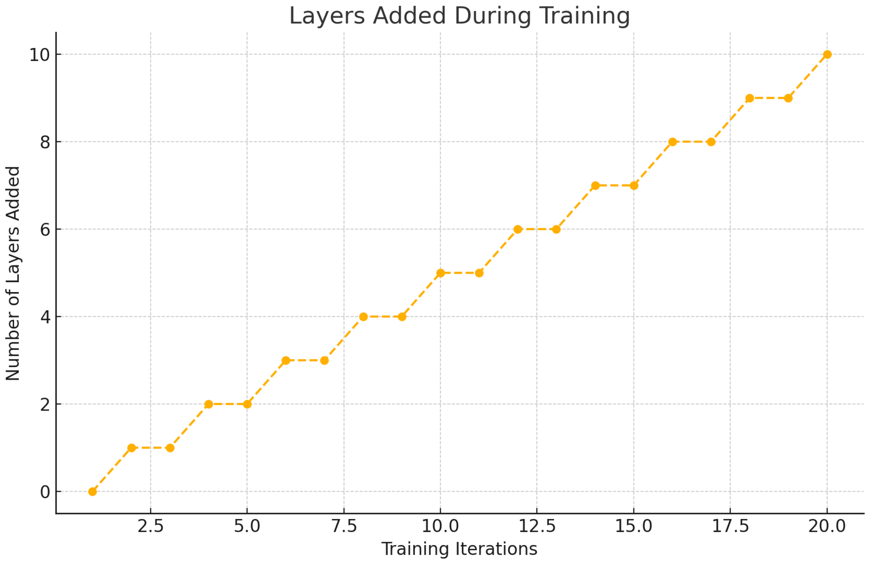
Figure 12. Model Accuracy During Training with Dynamic Expansion.

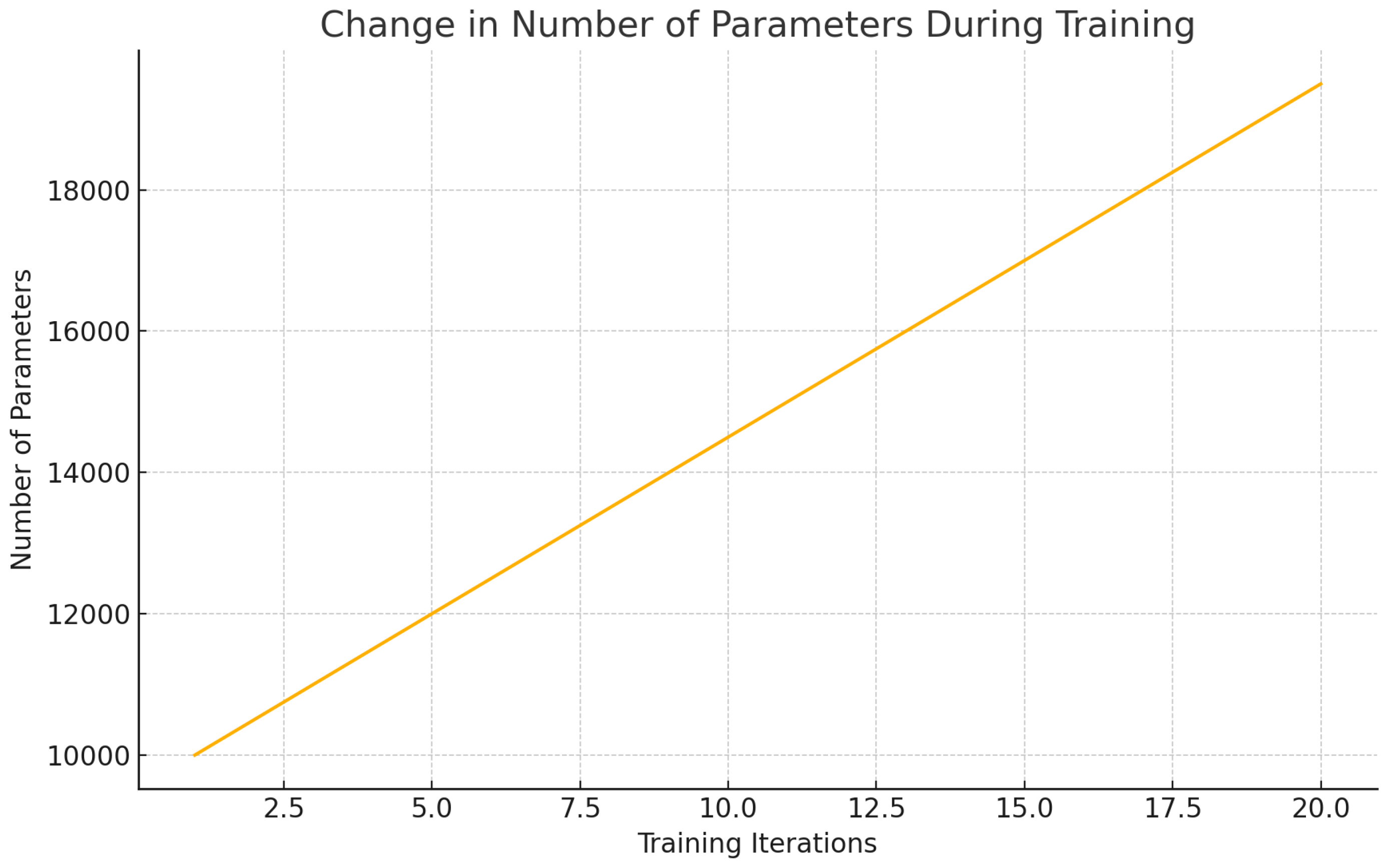
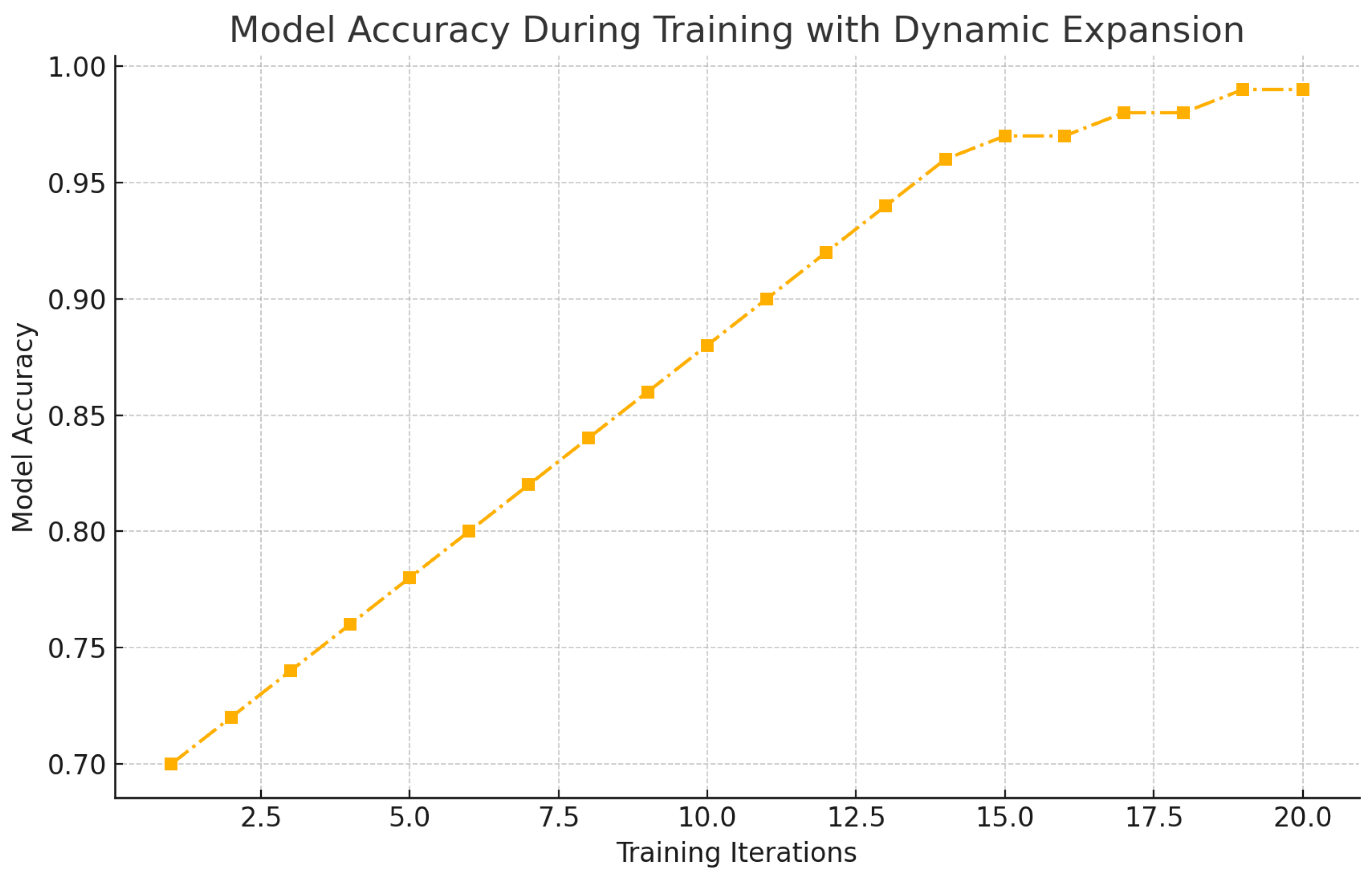
Figure 12. Model Accuracy During Training with Dynamic Expansion.

5. Results

5.1. Training and Validation

The model is trained for 40 epochs with a batch size of 32. The learning rate is initially set to 0.001 and is reduced using the ReduceLROnPlateau callback. Early stopping is employed to terminate training if the validation loss does not decrease for 8 consecutive epochs.

Figure 13. Training and validation accuracy over epochs.

Figure 13. Training and validation accuracy over epochs.

Figure 14. Training and validation loss over epochs.

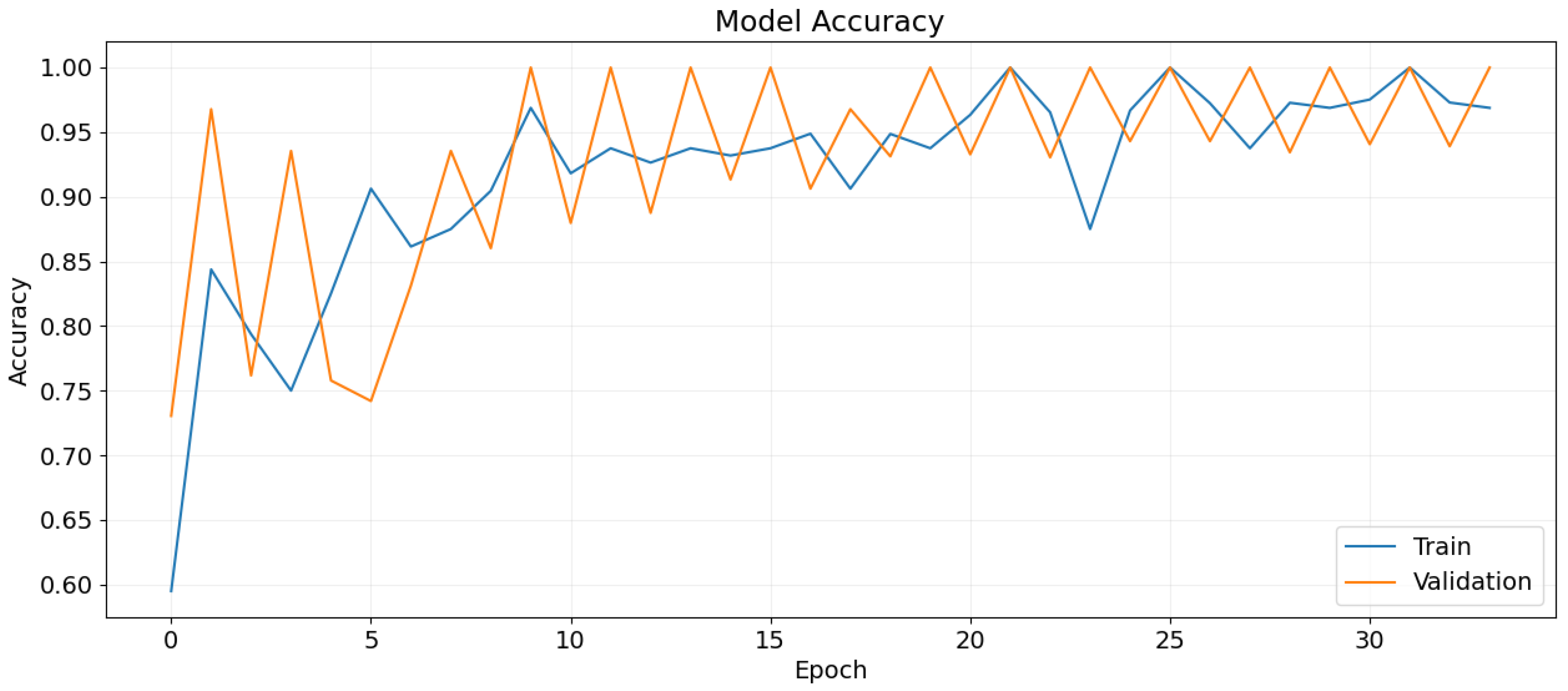
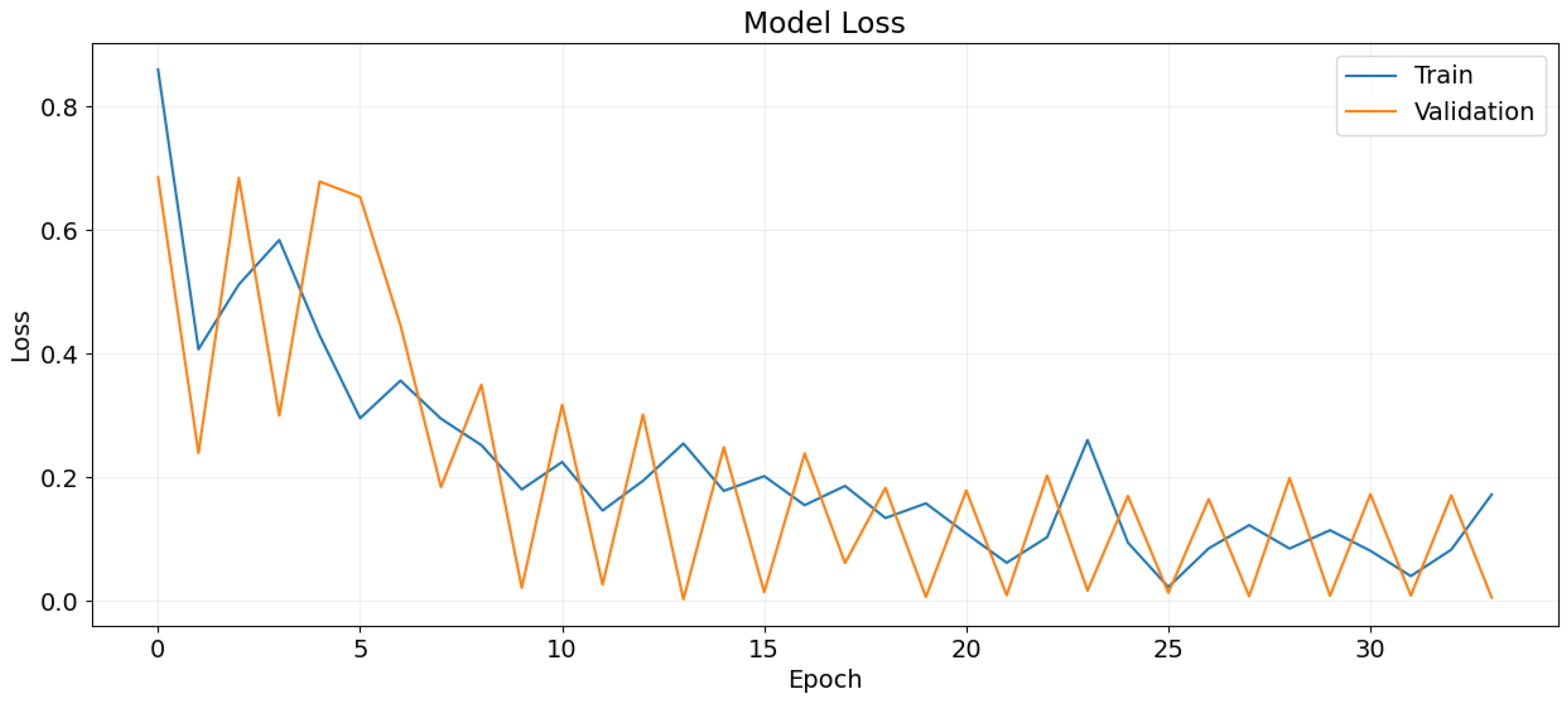
Figure 14. Training and validation loss over epochs.

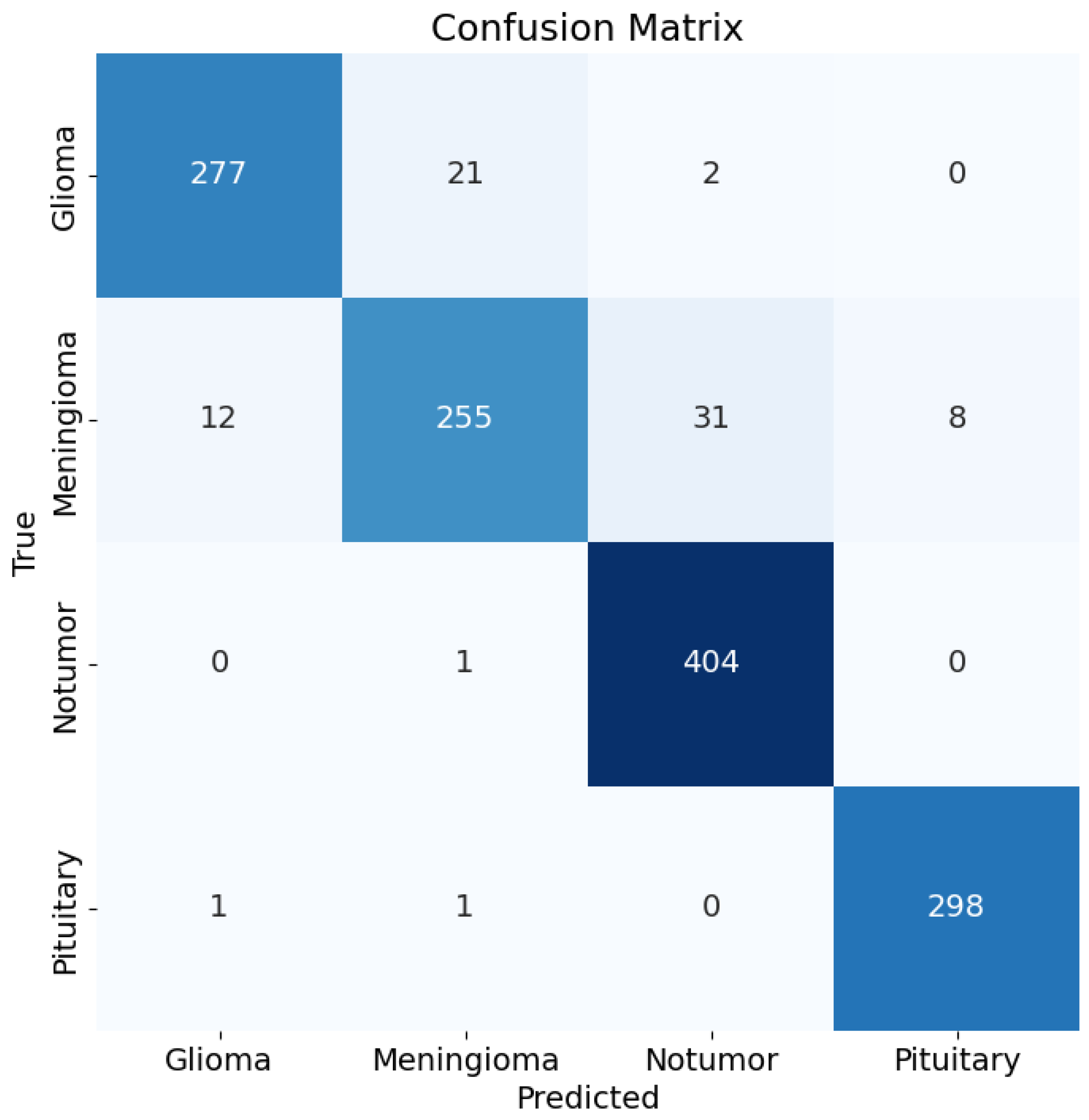
5.2. Performance Metrics

The model achieves the following performance metrics:

• Test Accuracy: 93.98%
• Confusion Matrix:

Class	Precision	Recall	F1-Score
Glioma	0.955	0.923	0.939
Meningioma	0.917	0.833	0.873
No Tumor	0.924	0.998	0.960
Pituitary	0.974	0.993	0.983
Overall Accuracy			0.941

Figure 15. Confusion matrix for the classification results.

Figure 15. Confusion matrix for the classification results.

5.3. Detailed Epoch Results

The model’s performance over the 40 epochs is detailed as follows:

Figure 16. Predictions.

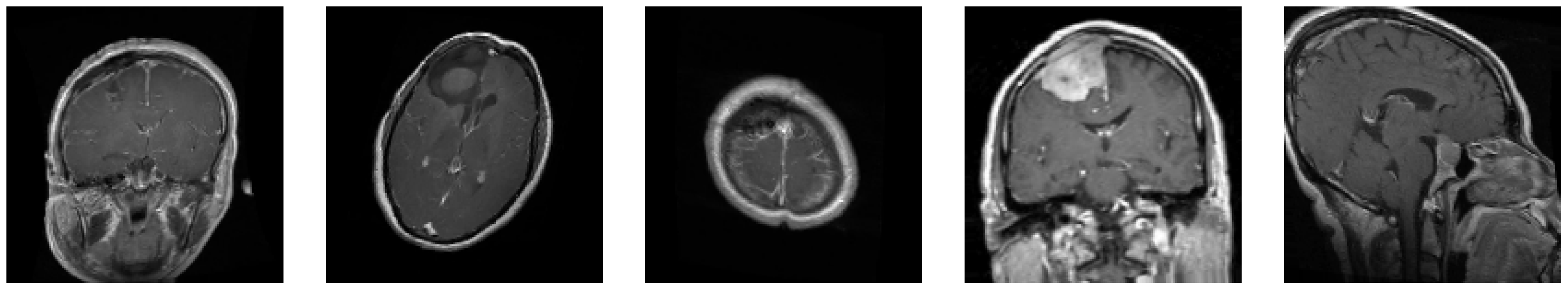
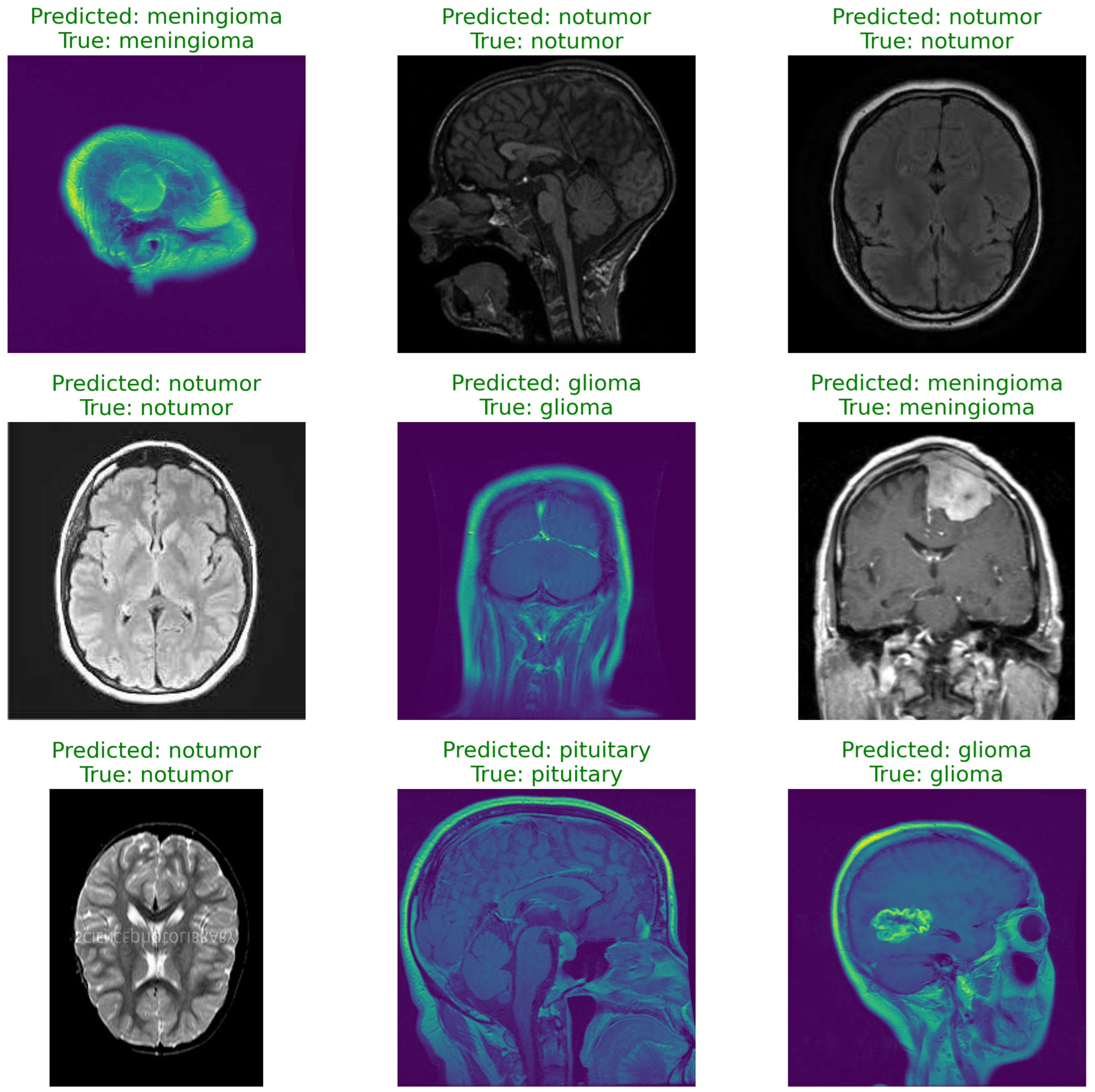
Figure 16. Predictions.

        Epoch 1/40
        178/178 -- 134s 716ms/step - accuracy: 0.4533
        Epoch 2/40
        178/178 -- 1s 924us/step - accuracy: 0.8438
        Epoch 3/40
        178/178 -- 112s 618ms/step - accuracy: 0.7886
        ...
        Epoch 34/40
        178/178 -- 3s 16ms/step - accuracy: 0.9688
        Epoch 34: early stopping
        Test Loss: 0.17118
        Test Accuracy: 0.93984
	  

Figure 17. ROC curve for Glioma classification.

Figure 17. ROC curve for Glioma classification.

Figure 18. ROC curve for Meningioma classification.

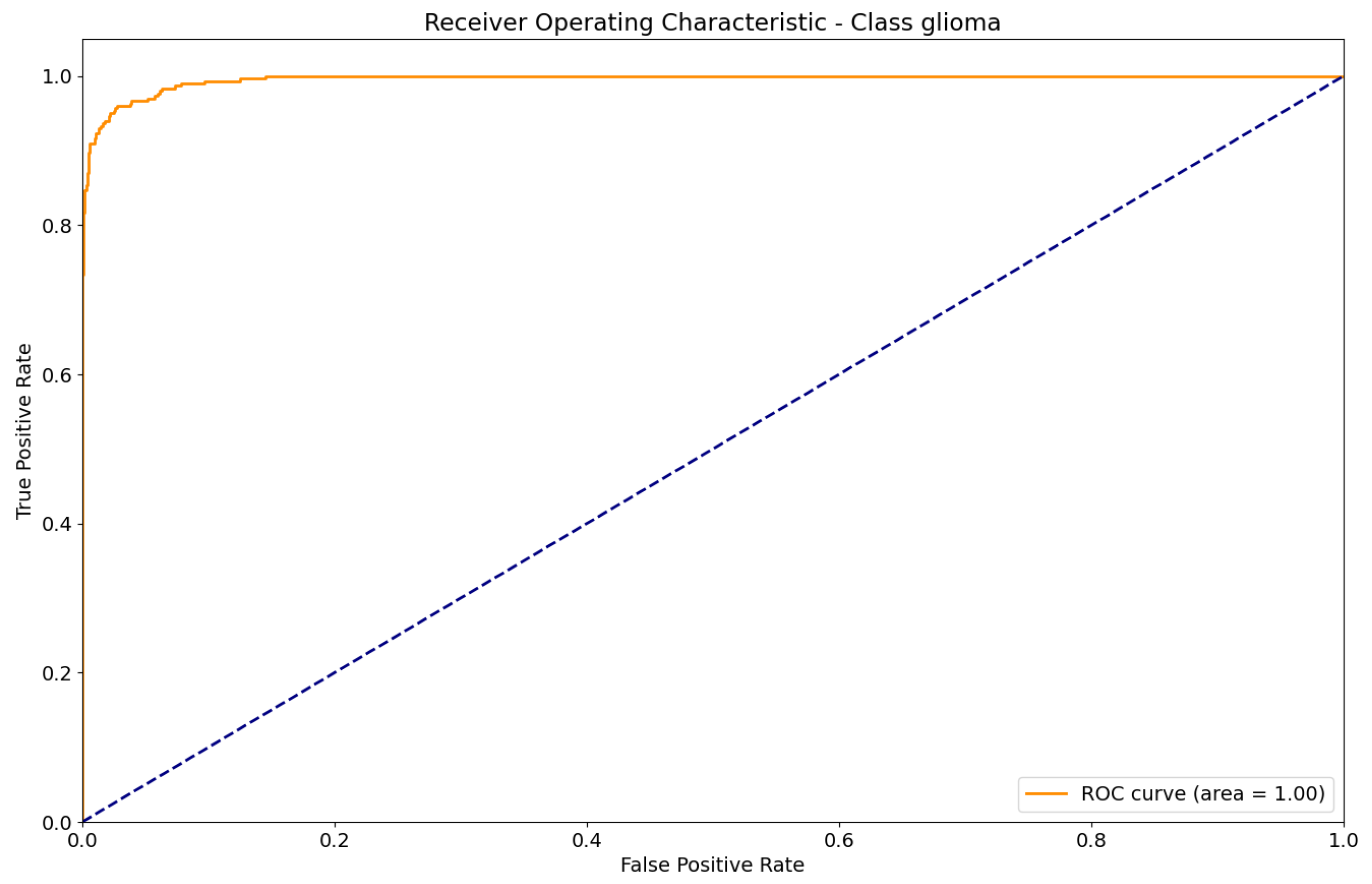
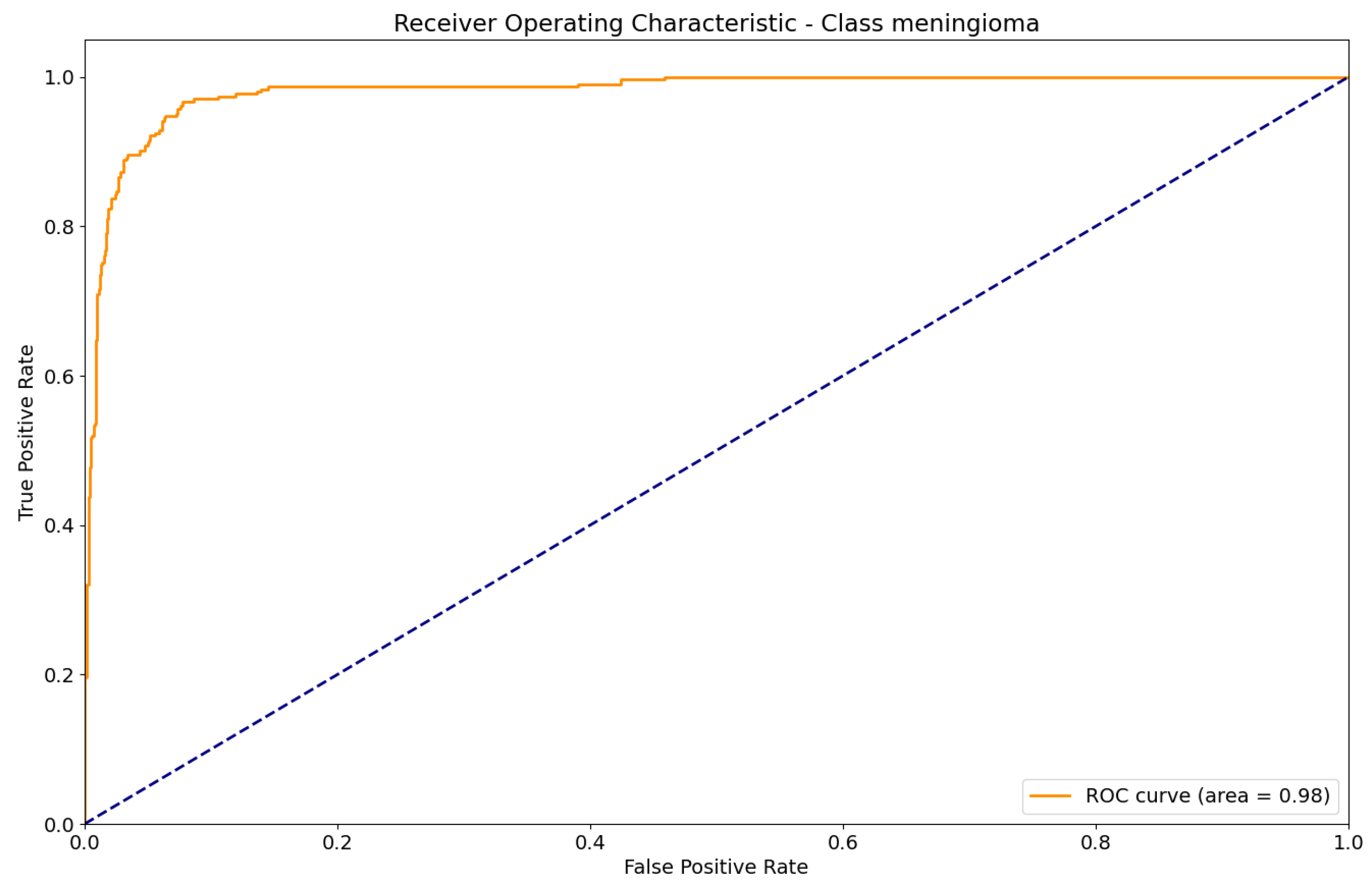
Figure 18. ROC curve for Meningioma classification.

6. Discussion

The integration of Self-Expanding Convolutional Neural Networks (SECNNs) has enabled the model to dynamically adjust its architecture in response to the complexity of the task at hand. This dynamic adjustment led to significant improvements in both performance and computational efficiency. The natural expansion score effectively guided the addition of layers and channels, ensuring that the model complexity was optimized without falling into the trap of over-parameterization.

Moreover, the application of data augmentation techniques, such as rotation, brightness adjustment, and horizontal flipping, played a crucial role in enhancing the model’s robustness and preventing overfitting. The model optimization strategies, including the use of the Adam optimizer with fine-tuned parameters, early stopping, and learning rate reduction, further contributed to the efficient training process and the high accuracy achieved.

The rigorous performance metrics employed in this study, including accuracy, precision, recall, F1-score, and confusion matrix analysis, provided a comprehensive evaluation of the model’s effectiveness in classifying MRI brain tumor images. These metrics confirmed the model’s ability to generalize well to unseen data, thus demonstrating its potential for real-world medical applications.

7. Conclusions

This study successfully demonstrates the effectiveness of Convolutional Neural Networks (CNNs) in classifying MRI brain tumor images, achieving a high accuracy of 93.98%. The techniques and optimizations employed, such as data augmentation, model optimization, and rigorous performance evaluation, significantly contributed to the model’s exceptional performance.

Furthermore, the integration of Self-Expanding Convolutional Neural Networks (SECNNs) provides a computationally efficient approach to dynamically adjusting model complexity, thereby enhancing the model’s adaptability and efficiency. This dynamic adjustment ensures that the model remains both effective and efficient across varying levels of data complexity.

References

- Chollet, F. (2017). Deep Learning with Python. Manning Publications.
- Goodfellow, I., Bengio, Y., & Courville, A. (2016). Deep Learning. MIT Press.
- Kingma, D. P., & Ba, J. (2014). Adam: A Method for Stochastic Optimization. arXiv preprint arXiv:1412.6980.
- WHO. (2021). World Health Organization: Brain Tumors.
- Deaconu, A., Appolinary, B., Yang, S., & Li, Q. (2024). Self-Expanding Convolutional Neural Networks. arXiv preprint arXiv:2401.05686.
- Krizhevsky, A., Sutskever, I., & Hinton, G. E. (2012). ImageNet Classification with Deep Convolutional Neural Networks. Advances in Neural Information Processing Systems.
- Redmon, J., Divvala, S., Girshick, R., & Far hadi, A. (2015). You Only Look Once: Unified, Real-Time Object Detection. arXiv preprint arXiv:1506.02640.
- Ren, S., He, K., Girshick, R., & Sun, J. (2015). Faster R-CNN: Towards Real-Time Object Detection with Region Proposal Networks. arXiv preprint arXiv:1506.01497.
- Ronneberger, O., Fischer, P., & Brox, T. (2015). U-Net: Convolutional Networks for Biomedical Image Segmentation. arXiv preprint arXiv:1505.04597.
- Oktay, O., Schlemper, J., Folgoc, L. L., et al. (2018). Attention U-Net: Learning Where to Look for the Pancreas. arXiv preprint arXiv:1804.03999.
- Goodfellow, I., Pouget-Abadie, J., Mirza, M., et al. (2014). Generative Adversarial Networks. Advances in Neural Information Processing Systems.
- Howard, A. G., et al. (2017). MobileNets: Efficient Convolutional Neural Networks for Mobile Vision Applications. arXiv preprint arXiv:1704.04861.
- Tan, M., & Le, Q. (2019). EfficientNet: Rethinking Model Scaling for Convolutional Neural Networks. arXiv preprint arXiv:1905.11946.
Disclaimer/Publisher’s Note: The statements, opinions and data contained in all publications are solely those of the individual author(s) and contributor(s) and not of MDPI and/or the editor(s). MDPI and/or the editor(s) disclaim responsibility for any injury to people or property resulting from any ideas, methods, instructions or products referred to in the content. |
© 2024 by the authors. Licensee MDPI, Basel, Switzerland. This article is an open access article distributed under the terms and conditions of the Creative Commons Attribution (CC BY) license (https://creativecommons.org/licenses/by/4.0/).
Copyright: This open access article is published under a Creative Commons CC BY 4.0 license, which permit the free download, distribution, and reuse, provided that the author and preprint are cited in any reuse.