
Submitted:
19 October 2024
Posted:
21 October 2024
You are already at the latest version
Abstract
Angola has an enormous agricultural potential, but the challenge remains how the country can transform potential into real growth. This study is designed to analyze the impact of the agricultural sector on economic growth in Angola and suggest recommendations for a better policy framework of the agricultural sector for a structural growth of the economy. Annual time-series data from 1993 to 2022 were used. The ARDL and EC model were applied to analyze both long and short-term relationships, as well as different statistical and econometric tests were used to examine the significance of the input data and model results, including various diagnostic tests and the Granger causality test. The study findings show stronger evidence of a long-run relationship between the dependent and independent variables than in the short run. Short run results show to be statistically insignificant. Agricultural value added shows the best reaction in all lags involved, indicating that economic growth would, caeteris paribus, respond positively to improvement in agricultural performance in Angola, although delayed by 3 years. Agricultural value-added development would improve both the contribution of agricultural employment and agricultural exports towards economic growth, as well contribute to a better rural development in Angola.
Keywords:
Economic growth
; agriculture
; ARDL model
; Angola
INTRODUCTION
According to Food and Agriculture Organization of the United Nations (FAO), in 2021, Africa’s agricultural population was 48 percent of the total population (460 million), and the agricultural value added accounted for US$ 425 billion of its total gross domestic product (GDP), representing roughly 10 percent of its total GDP (FAO 2023). Food and non-food agricultural production has not only an economic impact, but also a political and social impact. Trajectories and performances are different from one country or region to another, between the main subsectors, between agri-climatic zones, according to production systems or between different types of producers. The contribution of the agricultural sector to the economic growth of countries with strong agricultural dependence is strongly interdependent with their population dynamics and their consequent economic and social challenges.
Angola’s economy was built by the Portuguese to be an export-oriented economy with strong agribusiness value chains. Before the independence in 1975, Angola was one of Africa’s major producer and exporter of cotton, corn, banana, tobacco, sugar cane, and sisal (Dilolwa, 2000, p. 156) and even became the 4th largest coffee exporter in the world, after Brazil, Colombia and Côte d’Ivoire with a share of 6.1 percent of world exports (Caetano João, 2005, p. 113). However, the contribution of local farmers to the overall agricultural value chain was limited. As shown in Figure 1 below, local smallholder farmers were mostly involved in the primary production, and European businessmen secured the rest of the value chain segments, including the exports. This experience did not build local capacity or bring skills to develop other segments of the value chain.
The independence of Angola from the Portuguese in 1975, in midst of the Cold War, triggered what evolved to be a long-lasting civil war, ending only in 2002. The civil war reversed the course of value chains, becoming an importer of almost 95% of the consumption needs, mostly food using extractive sector proceeds (oil and diamonds). Between 2015 and 2020, this economic model was challenged, as Angola experienced a strong financial and economic crisis resulting from the drop in oil revenues. To minimize these effects on the economy, the Government launched several initiatives, including credit to the productive sector, to diversify the economy, which involved increasing domestic production with a view of reducing imports and diversifying exports mainly of agribusiness products where Angola has comparative advantages.
The war had its effect on agricultural performance, showing that in 1996, during a short cease fire period, agriculture showed an outstanding performance. But with all these efforts in policy alignment and private sector response, in recent years, the contribution of agriculture to the Angolan economy has grown rapidly, leading to an increase in the share of agriculture in the GDP from 5.8 percent to 8.9 percent of GDP from 2011 to 2022. In 2002, as shown in Figure 2 below, agricultural value added grew 3.8 percent but in the last 20 years growth averaged 6.2 percent, as shown in graph Local production of agricultural goods accounts for less than 30 percent of its needs and the rest is imported.
However, notwithstanding this performance, only 15 percent of the overall arable land is currently cultivated, and 20 percent is suitable for irrigation. Agriculture in Angola is also commonly linked to poverty and inequality, hence less capacity to cumulate capital and scale up agricultural production. Millions of people live in poverty in the in rural areas. The main source of their income and employment derives from agricultural activity, and indirectly since the state of agriculture influences that of the rural non-agricultural economy. It is expected that food and non-food agricultural production help alleviate poverty in general, contributing significantly to general economic growth by feeding the agribusiness value chain and linking with other sectors of the economy.
Consequently, agriculture alone will struggle to contribute to economic growth and impact the development of the country. It needs investments and development in other fields or sectors to thrive. For this reason, an increase in agricultural production per se may not contribute to economic growth as it does in other countries with different stage of development.
Hence, this study analyses the contribution of agriculture performance on economic growth in Angola and what policies and measures would help boost its productivity.
1.1. Research questions
This research seeks to answer the following research questions:
- (i)
- Is there a long or short run relationship between agriculture and economic growth?
- (ii)
- What policy recommendations and policy measures could help enhance agricultural sector productivity to further unlock its diversification potential and take advantage of regional and international economic integration?
1.2. Research objectives
The main objective of this study is to examine and quantify the relationship of agriculture on economic growth in Angola. The investigation employs an Autoregressive Distributed Lag (ARDL) and subsequent diagnostic tests to examine the importance of agriculture in economic growth by short-run and long-run relationships, as well as the direction of causality. The bi-directional relationship analysis between agricultural sector growth and economic growth is fundamental to design and implementation of successful economic development policies in Angola.
Additionally, this study aims at analyzing agriculture development trends and international best practices, as well as review agricultural policies and policy measures in Angola.
1.3. Hypothesis
The following null and alternative hypothesis will be tested in accordance with the objectives of the dissertation to verify if the agricultural sector has an impact on economic growth during the period 2003 to 2022:
- H0: Agricultural sector growth does not have significant impact on economic growth in Angola; and
- Ha: Agricultural sector growth has significant impact on economic growth in Angola.
The hypothesis above will be verified on a 5 percent significance level in both short and long terms. If the probability of the t-value is more than the significance level the null hypothesis will be accepted. If the probability of the t-value is less than the significance level the null hypothesis will be rejected.
1.4. Significance of the research
The novelty of this study is that no prior studies assessing the impact of agriculture on economic growth in Angola were made. Its findings can support policymakers from Angola and its developing partners in conducting effective policies and policy measures to pursue a sustainable agricultural performance for both economic and social gains.
2. LITERATURE REVIEW
The competitiveness of an economy is usually linked to economic performance measured by economic growth. The main political goal of the country is to stimulate production as a necessary basis for economic and social development. The determinants of economic growth can change in space and time. Depending on the methodological or theoretical approach (exogenous or endogenous growth theory) or on the time span analysis (short-term, medium-term or long-term perspective), the set of specific factors (variables) related to economic growth that are often considered is quite wide (Barro, 1991; Sala-i-Martin, 1997). Factors commonly included in growth regression equations typically include such basic economic indicators as employment, inflation, current account balance, government debt, exports and imports, foreign direct investment, fixed capital gross formation, etc., but also others related variables such as the quality and quantity of a country's workforce, natural resources, technological development, or social and political factors. Many theoretical and empirical studies have analyzed the identification of the determinants of economic growth, in particular the correlation between agriculture and economic growth. Some studies showed positive and some other negative impact of agriculture on economic growth. However, most findings showed that strong agriculture activity leads to economic growth.
2.1. Generic studies
Johnston and Mellor (1961) were among the earliest to systematically examine the role of agriculture in economic growth. They argue that agriculture provides food, raw materials, and employment, contributing to both industrial and service sector growth. Their work highlights how agricultural productivity improvements can trigger a positive spillover into the broader economy, by increasing rural incomes and thus boosting demand for non-agricultural goods.
Timmer’s (1988) work focuses on how agriculture plays a central role in transforming economies. He argues that increased agricultural productivity is essential for economic development, especially in early stages of growth. By increasing productivity, countries can release labor and capital for industrialization, which leads to higher economic growth. Lewis’ (1954) dual-sector model examines the structural transformation between agriculture and industrial sectors. In his model, agriculture serves as a reservoir of labor that can be reallocated to the industrial sector without sacrificing food security, fostering rapid economic growth.
Schultz’s (1964) seminal work suggests that even traditional agricultural systems can experience significant productivity gains with the introduction of modern technologies and better resource management. He argues that investment in human capital, such as education for farmers, can drive agricultural productivity and thus contribute to economic growth. Mellor (1995) explores how agriculture can foster industrialization by generating savings, investment, and food surpluses that support urban and industrial expansion. His work emphasizes that growth in agriculture is crucial for labor-intensive industries, as it reduces food prices and raises wages.
Gollin et al. (2002) focus on how agricultural productivity differences can explain large portions of income disparities across countries. Their study highlights the importance of improving agricultural productivity in low-income countries as a way to bridge the income gap with developed countries. The work of Diao and Thurlow (2010) emphasizes that agriculture remains the most significant sector for African economies and is key to poverty reduction and economic growth. They argue that without productivity improvements in agriculture, overall economic development in Africa will be slow, given the large rural populations.
Christiansen et al. (2011) analyze the linkage between agricultural growth and poverty reduction. Their findings suggest that growth originating from agriculture is more effective in reducing poverty than growth from other sectors, especially in low-income countries where a large proportion of the population relies on agriculture. Tiffin and Irz (2006) research provide empirical evidence on the relationship between agriculture and economic growth in developing countries. The authors find that in many developing countries, agriculture-led growth is critical, but it becomes less so as economies diversify and mature.
2.2. Specific African Economies
In the case of the African economies, with substantially better farming conditions providing comparative advantages in agricultural products, most studies examined the link between the agricultural sector and economic growth or on the link between agricultural trade and economic growth. Very few studies examined the link between agricultural investments and economic growth. Valdés and Foster (2010) highlight the unique challenges that Sub-Saharan African countries face in leveraging agriculture for economic growth. They argue that while agriculture remains a critical driver for growth, the sector needs better infrastructure, market access, and supportive policy environments to reach its full potential. For the case of the Tunisian economy, Matahir (2012) took a different stand using time series Johansen co-integration on his study on the role of agriculture on economic growth and how it affects other sectors in the economy. The study results show positive impact, recommending policy makers to see agricultural sector as pivotal tool when analyzing inter-sectoral growth policies. When addressing the impact of investment agriculture on the agricultural output, Badibanga and Ulimwengu (2020) explore the impact of agricultural investment on economic growth and poverty reduction in the Democratic Republic of Congo (DRC). The authors develop and utilize a two-sector economic growth model to analyze the optimal allocation of investments between the agricultural and non-agricultural sectors to maximize overall economic growth and reduce poverty.
Phiri et al. (2020) examined the agriculture sector in Zambia as determinant of economic sustainability for the period from 1983 to 2017. An ARDL model was applied and prove that agriculture the impact of agriculture on economic growth in Zambia was substantial in both the short and long-run. Sanyang (2018) also analyzed the impact of agriculture on economic growth in Gambia, using an ECM and ARDL model to estimate the economic growth and found a significant positive effect of agriculture on economic growth in both the short- run and long-run. Furthermore, Runganga and Mhaka (2021) assessed the impact of agriculture on economic growth in Zimbabwe using the ARDL estimation technique for the period from 1970 to 2018. Results show that agricultural production has a positive impact on economic growth in the short run, and no impact in the long run. Bakari and Abdelhafidh (2018) investigates the relationship between agricultural investment and economic growth in Tunisia. The authors employ an ARDL cointegration approach to analyze how different components of agricultural investment influence the long-term and short-term economic growth of the country.
Many theoretical and empirical studies have also analyzed the correlation between financial credit and agricultural sector growth. Some have found positive impact, while others negative, but the literature’s general conclusion is that strong financial systems increase credit activity and, subsequently, lead to economic growth. For instance, Akram et al. (2008) proved a positive effect of agricultural sector credit on agricultural sector growth in Pakistan with an elasticity of agricultural credit in relation to poverty of −0.35 percent and –0.27 percent in the short term and long term, respectively. Caetano João and Castro (2023) examined the degree of elasticity between two variables, namely, agricultural credit and agricultural growth, in Angola in the period 2003–2022 using the ARDL model. Results showed that the impact of agricultural credit on the growth of the agricultural sector was positive and statistically significant.
3. RESEARCH STRUCTURE AND METHODOLOGY
3.1. Data sources, estimation period and econometric tool
The data used to estimate the time series in the present study were extracted from United Nations specialized agencies, namely the World Bank – WB (World Development Indicators), IMF WEO, FAOSTAT, as well as from Angolan statistical system, namely Angola Statistical Office (INE), Ministry of Finance (MINFIN), MINAGRIF and BNA. The time series data are annual, covering the period from 1993 to 2022, a total of 30 observations. According to Narayan (2005) and Wolde-Rufael (2010), ARDL models are applicable to small sample size ranging from 30 to 80 observations.
For the estimation exercise, STATA 14.2 econometric tool was used.
3.2. Determination of variables
The determination of the variables involved a combination of theoretical understanding, empirical evidence, data availability and statistical techniques based on the definition of the research question and literature review. Data was collected for five variables, namely as shown in Figure 3 below.
3.3. Research methodology and model design
The objective of this study is to evaluate the impact of agriculture on Angola's economic growth, through robust methods, with the estimation of an econometric regression model using the ARDL test. To verify the degree of the relationship between the variables in the model, the hypotheses below were raised.
H0: Agriculture has no impact on economic growth; and
Ha: Agriculture has an impact on economic growth.
The methodology used to quantify the impact of agriculture on economic growth using an ARDL model, was by:
- (i)
- Conducting a unit root tests (ADF) to check the stationarity of each time series variable. For the test the basic equation applied involves estimating the following regression model (Nkoro & Uko, 2016, p. 72):
- (ii)
- selecting the optimal lag length for the ARDL model, using Akaike Information Criterion (AIC) and specifying the long-run ARDL model equation:
- (iii)
- estimating short-run relationship adding the error correction term, which is that of the long-term regression but lagged from a period;
- (iv)
- performing the bounds testing for cointegration and estimating the long-run relationship as well as the short-run dynamics using the error correction model (ECM);
- (v)
- Conducting a series of diagnostic tests to validate the model, namely
- a.
- Normality of residuals (Jarque-Bera test)
- b.
- Multicollinearity test
- c.
- Serial correlation test (Breusch-Godfrey LM test)
- d.
- Heteroscedasticity (Breusch-Pagan test)
- e.
- Stability (CUSUM test)
- f.
- Granger causality test
4. DATA ANALYSIS, RESULTS AND DISCUSSION
Figure 4 below describes descriptive statistical values for economic growth, inflation, gross fixed capital formation, agricultural value added and trade openness. It is worth noting that detailed analysis revealed that GDP mean, and median values are the lowest among variables with 4.2837 and 3.8400, respectively. Its standard deviation (st. dev.), that is, deviation of individual data points from the mean (average) is also the lowest with 7.7516 and the range of values goes from -23.9800 (minimum) to 15.0300 (maximum). Despite very high variance in the difference between minimum and maximum values across all variables, GDP, followed by agricultural value added, have the smallest difference with 39.01 and 95.32, respectively. The TO skewness and kurtosis values of 4.5617 and 24.0801, respectively, show that values are asymmetrical (skewed) and with irregular distribution. The skewness and kurtosis values of other variables show less asymmetrical distribution, being the GDP the closest to 0.
4.1. Optimal lag selection
According to the results of the information criterion (ANNEXURE C), the AIC criterion is found to be the most appropriate as it is the one with the least value. Results suggest that the most ideal lag for each variable of model ARDL is 1, 4, 2, 4, 0 for variables GDP, INF, GFCF, AgrVA and TO, respectively.
4.2. Unit root tests
As stated above, this study employs the ADF test to assess the stationarity of the series.
Dickey-Fuller unit root test results shown in Figure 5 indicate that variables are integrated at different order and statistically significant at 1 percent level, so cointegration test will be performed.
4.3. ARDL bound tests results for Cointegration
As seen above, series are integrated of different orders, that is with a combination of I(0) and I(1) series, hence the ARDL bounds test is applied on the level of the variables to determine whether the variables have a long-run cointegration.
Since the F-statistic of 4.922 is greater than the upper bounds critical values (3.52, 4.01, 4.49) at all significance levels (2.5, 5 and 10 percent), except at 1 percent significance level (5.06), the null hypothesis of no cointegration is rejected. Figure 8 confirms that there is a cointegrating relationship between the variables in the long run at 5% significance level. So, the ARDL model will be retained.
4.4. ARDL model estimation results
Variables GDP, INF, GFCF, AgrVA and TO are cointegrated and there is a long-run equilibrium relationship. The long and short-run models are therefore considered to be estimated.
4.4.1. Long-run relationship
With the existence of a long-run relationship between variables, the model will now quantify the effect of independent variables on the dependent variables, measuring the effect of explanatory variables on explained variable as shown in Figure 7.
Regression results analysis presents an R-squared value of 0.8646, which indicates that 86.46 percent of the variation in GDP is explained by the independent variables INF, GFCF, AgrVA and TO in the model. The adjusted R-squared value of 0.6614 accounts for the number of variables in the model, suggesting that after penalizing for the number of predictors, around 66.14 percent of the variation in GDP is still explained. The F-statistic of 4.26 tests the overall significance of the model. A probability (Prob > F) of 0.0129 means that the model is statistically significant at the 5 percent level, as this value is less than 0.05. Furthermore, the Root MSE value of 3.1434 represents the standard deviation of the residuals, indicating the model's prediction error.
Current GFCF and GFCF L1 show positive effect on GDP, especially current GFCF with a coefficient of 0.260681 and statistically significant p-value of 0.041, suggesting that an increase in GFCF positively affects GDP. But AgrVA has by large the most positive effect over GDP in current and all 4 lags. The largest coefficient is found in the current lag (.5231656) but it is marginally significant with a p-value of 0.092. The lagged term AgrVA L3 is significant (p = 0.033), reinforcing that past agricultural performance positively affects GDP. Other lagged AgrVA terms do not show significant effects.
4.4.2. Short-run relationship
Notwithstanding the fact that ARDL model confirmed long-run relationship between independent and dependent variables, understanding the short-term relationship between independent variables and a dependent variable is crucial in econometric and time series analysis for their ability to provide immediate insights and predictive power, inform policy and business decisions, enhance model accuracy, and align with economic theories.
Based on the ARDL short-run dynamics and ECM results, the R-squared value of 0.6957 indicates that approximately 69.57 percent of the variation in dGDP (dependent variable) is explained by the independent variables (dINF, dGFCF, dAgrVA, dTO, and ECT). This suggests a moderately good fit. Furthermore, the Adjusted R-squared value of 0.3361 demonstrates that after adjusting for the number of predictors, the explanatory power decreases to 33.61 percent, indicating that some independent variables may not significantly contribute to the explanation of the variation in dGDP. According to Narayan and Symth (2004), the result shows that the model corrects the previous period disequilibrium at a speed of 111 percent, thus overcorrecting the disequilibrium to achieve the long-run equilibrium steady-state position. Error correction terms between –1 and –2 indicate that the equilibrium is reached in a declining fluctuating mode.
The dAgrVA positive coefficient of 0.1896 indicates a positive relationship between agricultural value-added and GDP growth. However, this effect is also not statistically significant as the p-value of 0.270 is higher than the 5 percent significance level (0.05). Looking at the error correction term (ECT), indicating the speed of adjustment towards long-term equilibrium, the coefficient of –0.7702 suggests that approximately 77 percent of the disequilibrium from the previous period's shock is corrected in the current period. However, the p-value of 0.181 shows that this correction term is not statistically significant. Nevertheless, the F-statistic (Prob > F) value of 0.1401 also shows that it is not statistically significant at the 5 percent significance level (0.05). This means that the overall regression is not significant, and the model in the short run may not explain the dependent variable sufficiently.
4.5. Diagnostic tests results
Following the methodology outlined in chapter 4, diagnostic tests will be performed through (i) normality, (ii) autocorrelation, (iii) heteroscedasticity and (iv) stability tests.
4.5.1. Normality tests
According to Figure 9 above, the Jarque-Bera Statistic of 4.352 was calculated based on the skewness and kurtosis of the residuals and the higher this value, the greater the deviation from normality. When interpretating data skewness (–0.413), the residuals are slightly negatively skewed, indicating a small leftward asymmetry. However, the skewness is close to zero, suggesting near symmetry. On the other hand, the kurtosis value of 4.826 is greater than 3, which indicates that the residuals have heavier tails than a normal distribution (i.e., more extreme values). However, this value is not excessively high. This test result supports the adequacy of the model in terms of normally distributed residuals, which is a crucial assumption for many types of regression analyses.
4.5.2. Multicollinearity test
Results in Figure 10 indicate that AgrVA (1.67), INF (1.38), GFCF (1.29), and TO (1.14) are all under 10, which is the conventional threshold for multicollinearity. A VIF below 10 suggests there is no significant multicollinearity in the data, meaning that the predictor variables are not highly correlated with each other.
The mean VIF of 1.37 () indicates low multicollinearity, implying that the predictors do not strongly correlate with each other and are not inflated due to multicollinearity. This suggests that the model is well-specified, and the individual contributions of AgrVA, INF, GFCF and TO can be interpreted with confidence.
4.5.3. Autocorrelation test
Since the p-value of 0.2471 is greater than the typical significance level of 0.05, the null hypothesis of no autocorrelation is rejected. This suggests that there is no evidence of autocorrelation in the residuals of the model at lag 1. This implies that in simpler terms, the residuals appear to be uncorrelated, indicating that the model does not exhibit signs of serial correlation at the first lag.
4.5.4. Heteroscedasticity test
Figure 12.
White’s test for heteroscedasticity. Source: Author’s computation using STATA 14.2.

Since the p-value of 0.519 is greater than the 0.05 significance level, the null hypothesis is not rejected. This means that there is no evidence to suggest the presence of heteroscedasticity in the regression model. In other words, the assumption of constant variance in the residuals appears to hold. This result implies that the residuals' variance is consistent across observations, making the model reliable under the assumption of homoscedasticity.
4.5.5. Stability tests
Figure 13.
CUSUM test results. Source: Author’s computation using STATA 14.2.
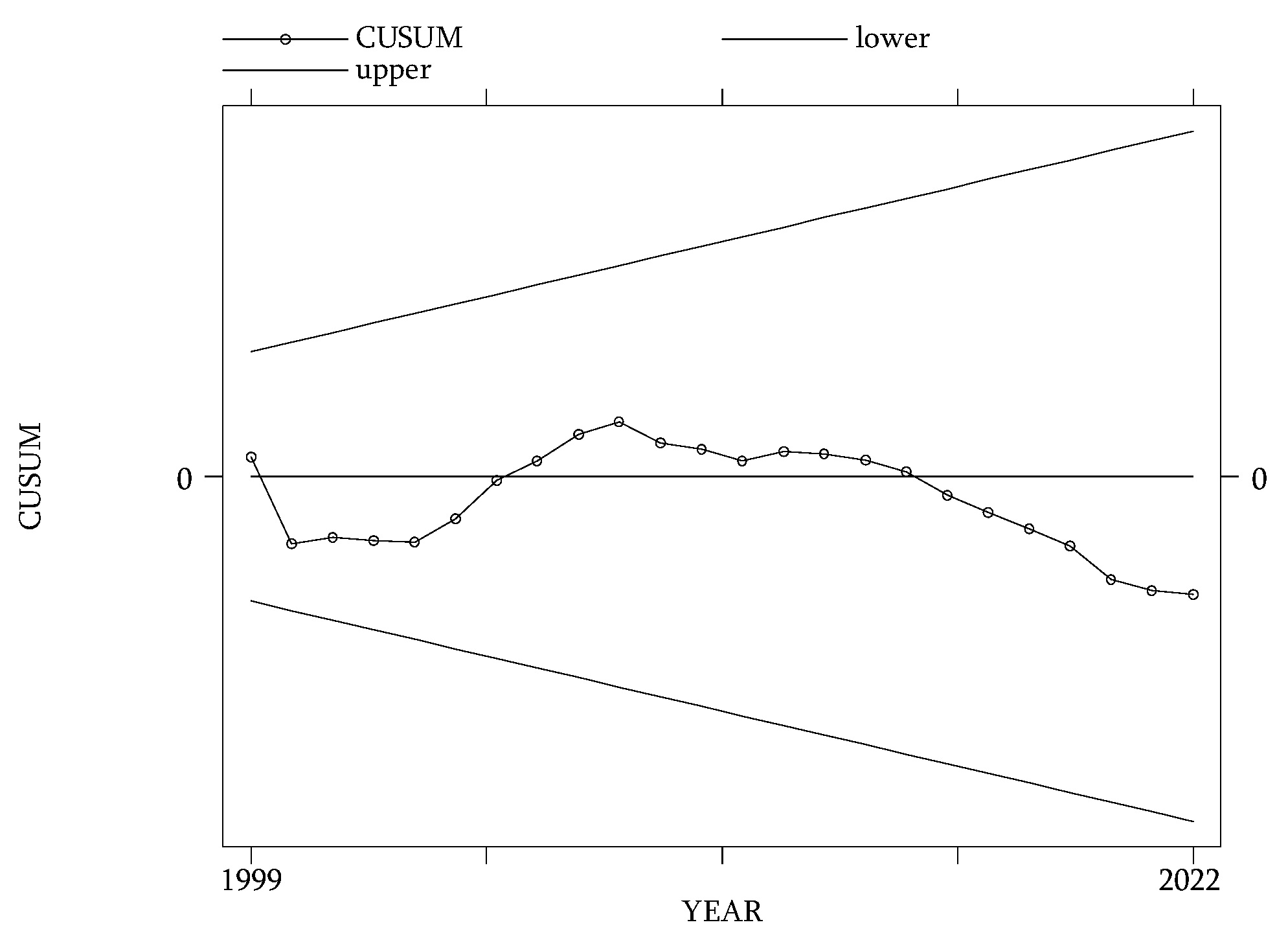
As part of the data stability assessment of the model, the cumulative sum of recursive residuals (CUSUM) test was performed to avoid model misrepresentations. Results show model stability as the CUSUM test results displayed in graph 54 is within the limits of 5 percent significance level. The ARDL model is stable, and stability exists within the model parameters.
4.6. Causality analysis results
Further analysis was made using the Granger causality test for the variables of the estimated ARDL model to determine the existence of a causal relationship between explanatory and dependent variables.
Figure 15.
Granger Causality Test.
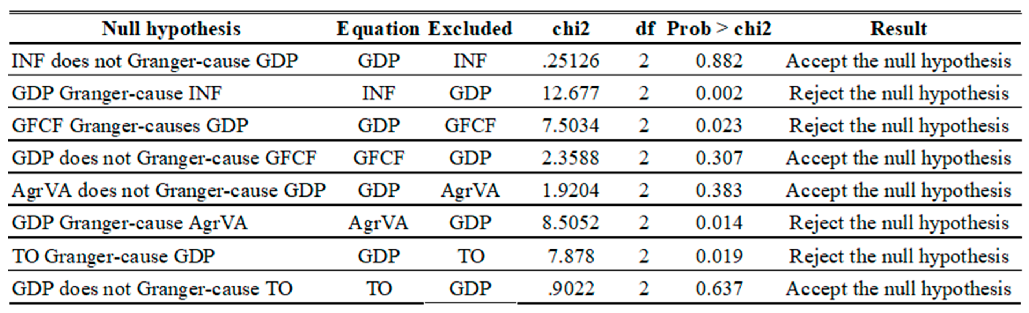
Granger tests results suggest a mix of unidirectional and bidirectional causalities. Investments (GFCF), trade openness (TO), and GDP influence different variables, but inflation and agricultural value-added do not seem to significantly impact GDP, though GDP impacts both inflation and agriculture. These results offer important insights for policy, particularly regarding the roles of investment and trade in economic growth.
4.7. Discussion
From the model point of view, the long run ARDL (1, 4, 2, 4, 0) model examines the impact of various lagged values of GDP, inflation, gross fixed capital formation, agricultural value-added, and trade openness on GDP. The lag structure captures both immediate and delayed effects of the explanatory variables on GDP. The objective of this research was to analyze the impact of agricultural value-added in economic growth in Angola and results address this concern. The structure of the long-run model has a good fit, with an R-squared of 86.46 percent, suggesting that the variables explain most of the variation in GDP. When examining the significance, although the overall model is significant (Prob > F is 0.0129), most of the individual variables are not statistically significant at the conventional 5 percent level. This means that, despite the model being generally good, most of the individual predictors cannot be reliably said to affect GDP in this specific sample period.
Looking at the key long-run results of the long run model estimation model, the GDP coefficient suggests that past GDP has little impact on current GDP. The coefficients for inflation are mostly statistically not significant, indicating that inflation may not have a strong effect on GDP in this context. From the GFCF perspective, the current period coefficient is significant (p = 0.041) and positive, implying that increases in GFCF positively impact GDP. Furthermore, AgrVA current and third lag coefficients are significant (p = 0.033 and p = 0.092, respectively), indicating a positive relationship with GDP, particularly with recent values. The TO coefficient is insignificant (p = 0.977), suggesting no impact on GDP and the constant term is –7.2444 with a p-value of 0.055, indicating that it is marginally significant. This may suggest a baseline effect on GDP that may warrant further investigation.
The economic significance of the coefficients is important. The presence of significant lags, such as the third lag for AgrVA, suggests a long-run equilibrium relationship, where agriculture influences GDP growth over a prolonged period. The significant lagged effect of agricultural value-added indicates that agricultural policies aimed at increasing productivity may take several years to show full effects. Therefore, long-term investment in agriculture could be crucial for sustained economic growth as a 1 percent increase in agricultural value-added is associated with a 0.319 percent increase in GDP after three years. This highlights the critical role of agriculture in driving long-term growth. These findings suggest targeted economic policies focusing on investment and agriculture could be beneficial for economic growth.
When interpreting the implications of non-significant coefficients, it should not be interpreted as the variable is unimportant. It may imply other relationships or that the effects are absorbed by other variables. For example, the insignificance of inflation may suggest that other factors, such as foreign exchange, external trade or global inflation trends might offset its impact on domestic GDP growth.
When analyzing the short run dynamics, only third lag of dAgrVA shows marginal statistical significance in impacting the GDP, emphasizing the importance of investment in agricultural productivity to foster economic growth. The non-significance of other variables suggests that not all factors have a meaningful influence on GDP in this context. When measuring the speed of adjustment back to long-run equilibrium after a short-run shock, the ECT coefficient (–0.7702) is found negative, as expected, which means the model is moving toward equilibrium in the long run. In practical terms, it takes approximately 1.3 years for the model to recover from short-term shocks (1/0.7702 = 1.298). But this adjustment is not statistically robust since the p-value (0.181) shows that the ECT is not statistically significant. The possible implications are that although the ECT has the expected negative sign, its lack of significance may imply weak long-run dynamics or that shocks to the system take longer to dissipate.
Theoretically, several factors can contribute to a positive relationship between GDP and agriculture, particularly in economies where agriculture plays a significant role like Angola. Some of these factors are technological advancements, human capital development, agricultural investments and capital accumulation, government policies and institutional support, market access and trade, and other.
Similar findings on the positive impact of agriculture on economic growth are found in Msuya (2007) on Tanzania, Izuchukwu (2011), Odetola et Etumnu (2013), Oyakhilomen and Zibah (2014), and Sertoğlu et al. (2017) on Nigeria, Moussa (2018) on Benin, Awokuse and Xie (2015) on Brazil, Chile, Mexico, China, Indonesia, Thailand, Kenya, South Africa, and Cameroon, Sanyang (2018) on Gambia, Runganga and Mhaka (2021) on Zimbabwe, Awan and Aslam (2015) on Pakistan, Phiri et al. (2020) on Zambia, Bakari and El Weriemmi (2022) on different Arab countries, and Bakari, S., & Abdelhafidh, S. (2018) on Tunisia.
5. CONCLUSIONS
5.1. Summary conclusions
This research has examined the impact of agricultural sector on economic growth in Angola using data from 1993 to 2022. When analyzing data, the ARDL bounds testing for cointegration approach was utilized. The ARDL bounds test was performed to assess if variables in the model have a long-run equilibrium relationship. The ARDL (1, 4, 2, 4, 0) model results indicate that gross fixed capital formation (GFCF) has an immediate and significant positive effect on GDP, suggesting that investment in physical capital plays a crucial role in driving short-term economic growth. On the other hand, agricultural value-added (AgrVA) shows a delayed but significant effect on GDP, particularly at the third lag, indicating that the agricultural sector's contributions to growth manifest over time. None of the lags of inflation or trade openness are significant, suggesting these factors do not directly influence GDP in the periods studied. The overall high R-squared (0.8646) shows that the model fits the data well, but the significance of lagged variables highlights the need for long-term planning and sustained investment, especially in agriculture and capital formation, for continued economic growth.
The Error Correction Model (ECM) results provide insights into both short-term dynamics and long-run equilibrium adjustment for GDP. While the error correction term is negative, as expected, it is not statistically significant, suggesting that adjustments back to long-run equilibrium after a shock are not rapid or robust in this context. The short-run dynamics indicate that inflation, capital formation, and trade openness have no statistically significant impact on GDP in the short term. However, agricultural value-added shows a marginally significant positive effect after three periods, hinting that agriculture may play a delayed role in influencing short-run GDP growth. Overall, the model highlights weak short-term relationships and a slow adjustment to long-term equilibrium, which calls for further investigation into the underlying dynamics of GDP growth. The diagnostic tests indicate that the model is robust and well-specified. The residuals are normally distributed, there is no significant multicollinearity, and the residuals show no evidence of autocorrelation or heteroscedasticity. Furthermore, the model demonstrates overall stability, as confirmed by the cumulative sum of recursive residuals (CUSUM) test.
5.2. Policy recommendations
Based on the ARDL short and long-run results from the research on the agricultural sector's impact on Angola's economic growth, several policy recommendations can be drawn to support sustained economic development. Given that gross fixed capital formation (GFCF) has a significant positive impact on GDP in the short term, the Angolan government should prioritize public and private investments in infrastructure, machinery, and industrial capital. Additionally, to that, it is advisable to strengthen long-term investment in the agricultural sector to realize its delayed but significant impact on economic growth. This can include funding for modern farming techniques, irrigation systems, research and development (R&D), and extension services for farmers. On the other hand, building capacity for processing and value addition in agriculture (value chains), especially for high-potential crops such as cassava, coffee, maize, and livestock is extremely important. Still in the value chains, improving rural infrastructure, such as roads, storage facilities, and market access points, to support agricultural productivity and reduce transaction costs for farmers is of capital importance.
When looking at the ECT results and its statistical insignificance, it is advisable to implement structural reforms aimed at improving the efficiency of institutions and markets to enable faster adjustments to economic shocks. This may include improving governance, reducing regulatory barriers, and increasing financial market accessibility. Furthermore, even though inflation did not show a direct impact on GDP, maintaining low and stable inflation rates is essential for investor confidence and long-term economic planning.
In summary, the findings of this study suggest that while Angola can achieve short-term economic gains through increased capital formation, the agricultural sector holds the key to sustained long-term growth. Strategic investments in agricultural productivity, infrastructure, and governance reforms, combined with export diversification, will help solidify Angola’s economic growth trajectory over the coming decades. Addressing the slow adjustment to long-term equilibrium by streamlining economic governance and enhancing institutional efficiency will further boost Angola’s economic resilience.
5.3. Accomplishment of research objectives
The core objective of this study was to assess the impact of agriculture on economic growth in Angola, which was positive. Furthermore, this study addressed the following research questions:
- (1)
- “Is there a long or short run relationship between agriculture and economic growth?”
Subchapter 4.4 on the findings of the ARDL model estimation shows existence, in the long and short run of positive relationship between AgrVA and GDP. Among other independent variables, AgrVA shows itself to be the major determinant of economic growth with long run coefficients spanning from 0.2270528 to 0.5231656 (average 0.36369466), and a short run coefficients from 0.1896218 to 0.3141319 (average 0.1905213), which means that in average, 1 percent increase would result in the long and short-run in a, ceteris paribus, 0.36 and 0.19 percent increase of GDP, respectively. On the other hand, statistical significance show that impact delays in average 3 years (lag 3).
- (2)
- “What policy recommendations could help enhance agricultural sector productivity?”
Possible policy measures are addressed in subchapter 5.2, where, the findings of this research suggest that while Angola can achieve short-term economic gains through increased capital formation, the agricultural sector holds the key to sustained long-term growth. Strategic investments in agricultural productivity, infrastructure, and governance reforms, combined with export diversification, will help solidify Angola’s economic growth trajectory over the coming decades. Addressing the slow adjustment to long-term equilibrium by streamlining economic governance and enhancing institutional efficiency will further boost Angola’s economic resilience.
5.4. Limitations of the research
The main limitation of this study is that the data series is not sufficiently robust (long) to show more statistically significant results, especially when running the ARDL model 1, 4, 2, 4, 0, as some data were not available. The war in Angola, from liberation struggle to civil war lasted more than 40 years and institutional capacity in all angles was heavily compromised. One more limitation of the study was the availability of separate statistics for life stock, agriculture, fisheries, and forestry which forced the study to adopt aggregated statistics as a proxy for agricultural value added. It is worth noting that economic growth may also be affected by other variables other than those used in the regression exercise, such as infrastructure, including water and energy availability, and capacity building.
References
- Akram, W., Hussain, Z., Sabir, H., & Hussain, I. (2008). Impact of agriculture credit on growth and poverty in Pakistan. European Journal of Scientific Research, 23, 243–251.
- Awan, A., & Aslam, A. (2015). Impact of Agriculture Productivity on Economic Growth: A Case Study of Pakistan. Global Journal of Management and Social Sciences, 1(1), 57-71.
- Awokuse, T., & Xie, R. (2015). Does Agriculture Really Matter for Economic Growth in Developing Countries? Canadian Journal of Agricultural Economics/Revue canadienne d'agroeconomie, 63(1), 77-99.
- Badibanga, T., & Ulimwengu, J. (2020). Optimal investment for agricultural growth and poverty reduction in the Democratic Republic of Congo a two-sector economic growth model. Applied Economics, 52(2), 135-155.
- Bakari, S., & Abdelhafidh, S. (2018). Structure of Agricultural Investment and Economic Growth in Tunisia: An ARDL Cointegration Approach. Economic Research Guardian, Weissberg Publishing, 8(2), 40-64.
- Bakari, S., & El Weriemmi, M. (2022). Causality between Domestic Investment and Economic Growth in Arab Countries. MPRA Paper No 113079.
- Barro, R. (1991). Economic Growth in a Cross Section of Countries. The Quarterly Journal of Economics, 106(2), 407-443.
- Caetano Joao, M. (2005). Ekonomika angolského zemědělství. Caetano Joao, M., Jelinek, P., Knitl, A. (eds.) Lusofonní Afrika 1975-2005 África Lusófona. Ústav mezinarodních vztahů, 107-117.
- Caetano Joao, M., & Castro, A. (2023). The Impact of Agricultural Credit on the Growth of the Agricultural Sector in Angola. Sustainability, 15(20), No 14704.
- Christiaensen, L., Demery, L., & Kuhl, J. (2011). The (Evolving) Role of Agriculture in Poverty Reduction—An Empirical Perspective. Journal of Development Economics, 96, 239-254. http://dx.doi.org/10.1016/j.jdeveco.2010.10.006.
- Diao, X., Hazell, P., & Thurlow, J. (2010). World Development, 38(10), 1375-1383.
- Dilolwa, C. (2000). Contribuição à História Económica de Angola, (2nd ed.). Nzila.
- FAO (2023a). Gross domestic product and agriculture value added 2012–2021: Global and regional trends. FAOSTAT Analytical Brief 64. Acceded online: 14/06/2024:https://openknowledge.fao.org/server/api/core/bitstreams/c6828277-8ca4-43e4-9033-c28d488d1083/content.
- Gollin, D., Parente S., & Rogerson, R. (2002). The Role of Agriculture in Development. American Economic Review, 92(2), 160-164.
- Izuchukwu, O. (2011). Analysis of the Contribution of Agriculture Sector on the Nigerian Economy Development. World Review of Business Research, 1, 191-200.
- Johnston, B., & Mellor, J. (1961). The Role of Agriculture in Economic Development. The American Economic Review, 51, 566-593.
- Lewis, W. (1954). Economic Development with Unlimited Supplies of Labor. The Manchester School, 22, 139-191. [CrossRef]
- Matahir, H. (2012). The empirical investigation of the nexus between agricultural and industrial sectors in Malaysia. International Journal of Business and Social Science, 3(8), 225-230.
- Mellor, J. (1995). Agriculture on the road to industrialization. Johns Hopkins University Press.
- Moussa, A. (2018). Does Agricultural Sector Contribute to the Economic Growth in Case of Republic of Benin? Journal of Social Economics Research, 5(2), 85-93.
- Msuya, E. (2007). The Impact of Foreign Direct Investment on Agricultural Productivity and Poverty Reduction in Tanzania. MPRA paper No 3671.
- Odetola, T., & Etumnu, C. (2013). Contribution of Agriculture to Economic Growth in Nigeria. The 18th Annual Conference of the African Econometric Society, Accra, Ghana, 1-29.
- Oyakhilomen, O., & Zibah, R. (2014). Agricultural Production and Economic Growth in Nigeria: Implication for Rural Poverty Alleviation. The Quarterly Journal of International Agriculture, 53(3), 1-17.
- Phiri, J., Malec, K., Majune, S., Appiah-Kubi, S., Gebeltová, Z., Maitah, M., Maitah, K., & Abdullahi, K. (2020). Agriculture as a Determinant of Zambian Economic Sustainability. Sustainability, MDPI, 12(11), 1-14.
- Runganga, R., & Mhaka, S. (2021). Impact of Agricultural Production on Economic Growth in Zimbabwe. MPRA Paper No 106988.
- Sala-i-Martin, X. (1997) I Just Ran Two Million Regressions. American Economic Review, 87(2), 178-183.
- Sanyang, M. (2018). Does Agriculture have an Impact on Economic Growth? Empirical Evidence from the Gambia. European Journal of Business and Management, 10(24), 88-99.
- Schultz, T. (1964). Transforming Traditional Agriculture. Yale University Press.
- Sertoğlu, K., Ugural, S., & Bekun, F. (2017). The contribution of agricultural sector on economic growth of Nigeria. International Journal of Economics and Financial Issues, 7(1), 547-552.
- Tiffin, R., & Irz, X. (2006). Is Agriculture the Engine of Growth? Agricultural Economics, 35, 79-89. [CrossRef]
- Timmer, P. (1988). The Agriculture Transformation. Handbook of Development Economics, Vol. 1. Elsevier Science Publishers B.V.
- Valdés, A., & Foster, W. (2010). Reflections on the Role of Agriculture in Pro-Poor Growth. World Development, 38(10), 1362-1374.
Figure 1.
Angolan agriculture value chain before the independence/ Source: Author’s illustration.
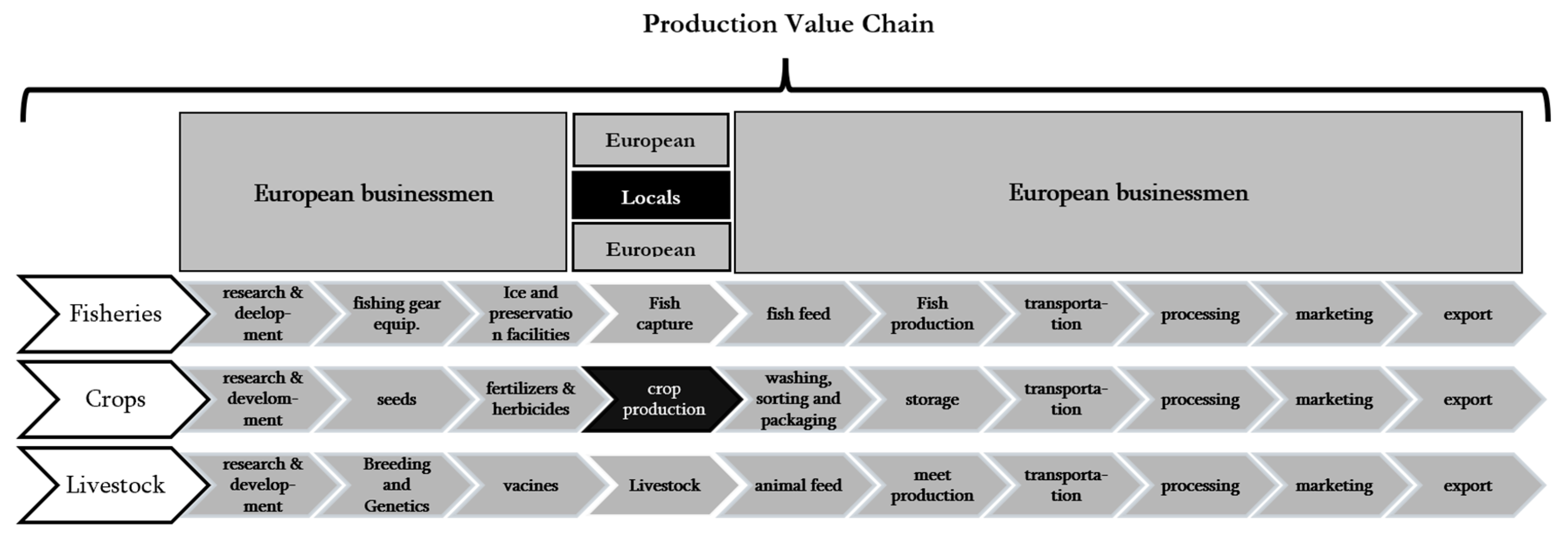
Figure 2.
Angola’s agricultural value-added performance in relation to GDP. Source: FAO and World Bank, online: https://databank.worldbank.org/reports.aspx?source=world-development-indicators#, 27/03/2024
Figure 2.
Angola’s agricultural value-added performance in relation to GDP. Source: FAO and World Bank, online: https://databank.worldbank.org/reports.aspx?source=world-development-indicators#, 27/03/2024
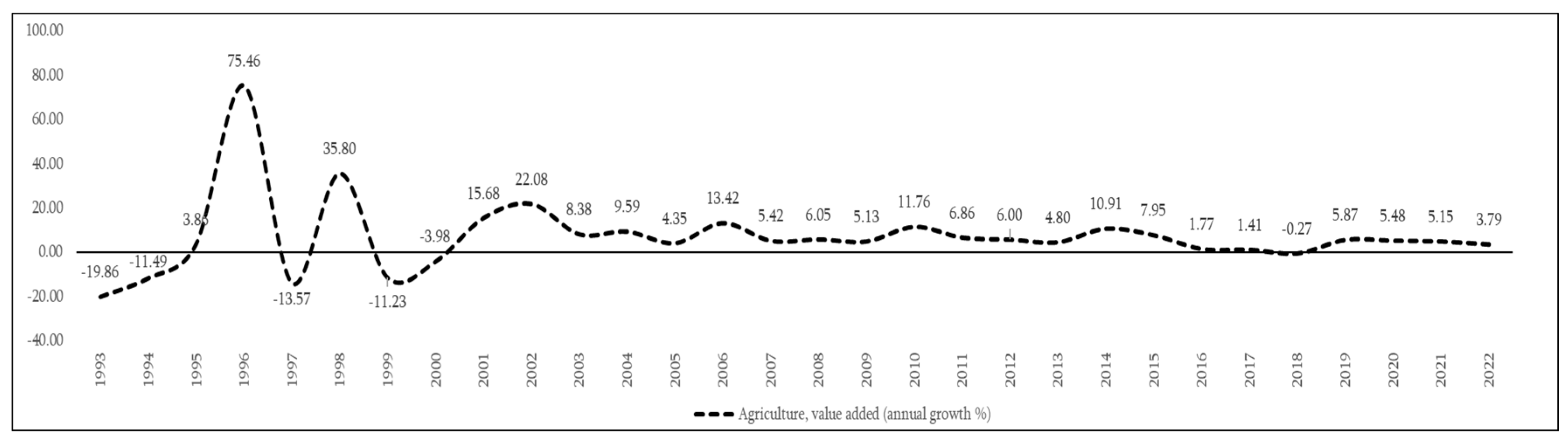
Figure 3.
Summary of dependent and independent variables used in the study.
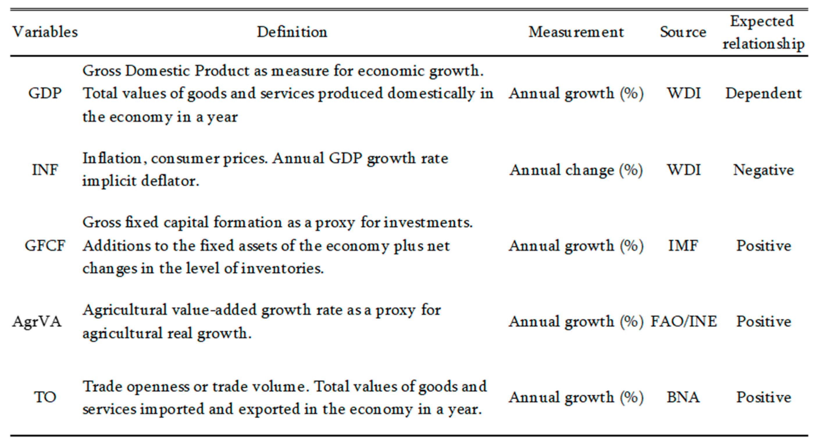
Figure 4.
Descriptive statistics results. Source: Author’s computation using STATA 14.2.
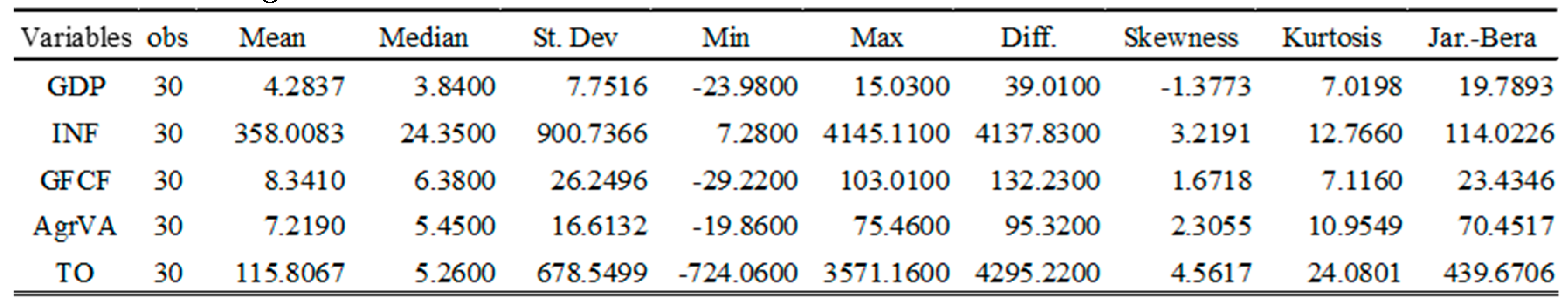
Figure 5.
ADF and PP unit root tests with constant and constant and trend. Source: Author’s computation using STATA 14.2.
Figure 5.
ADF and PP unit root tests with constant and constant and trend. Source: Author’s computation using STATA 14.2.
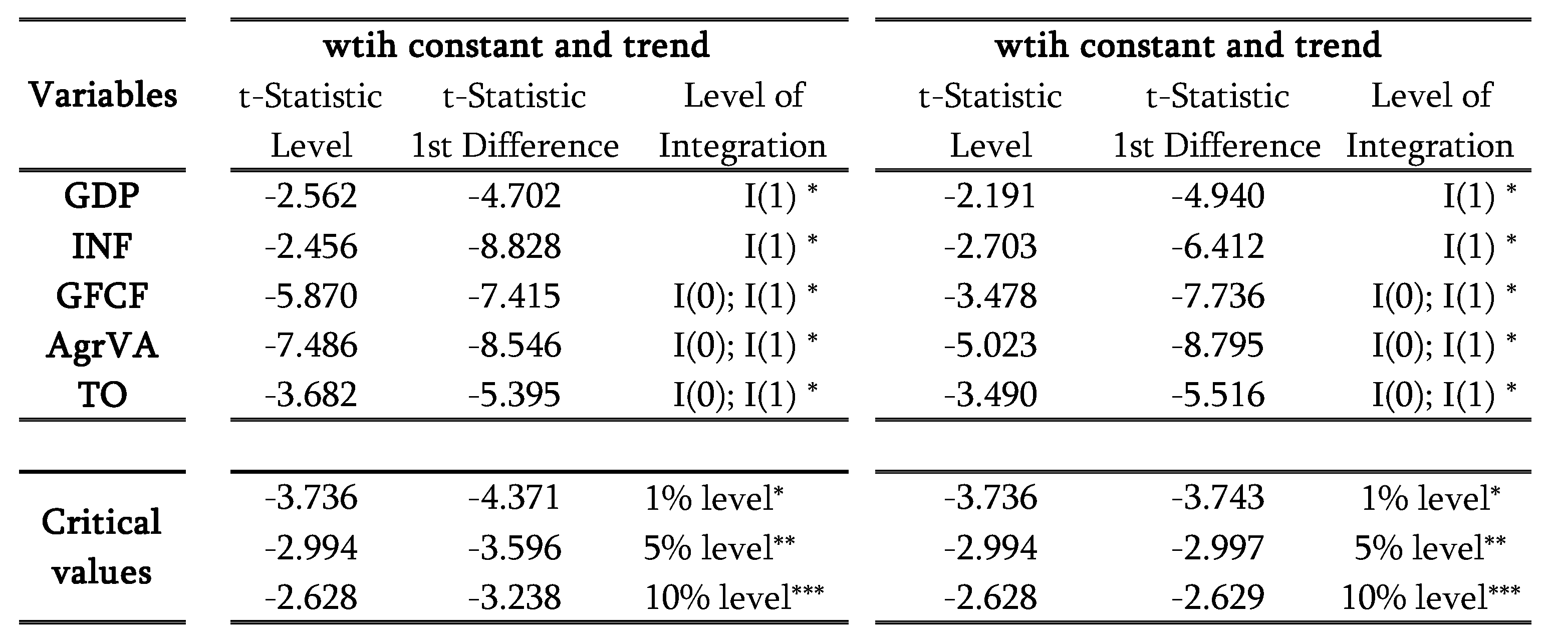
Figure 6.
ARDL bounds testing. Source: Author’s computation using STATA 14.2.
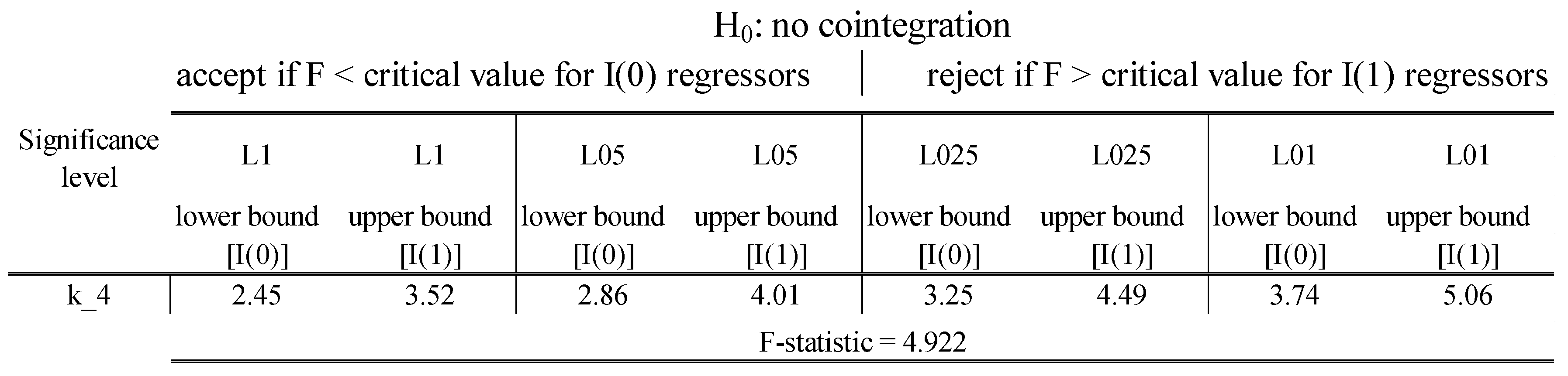
Figure 7.
Long run estimation results. Source: Author’s computation using STATA 14.2.
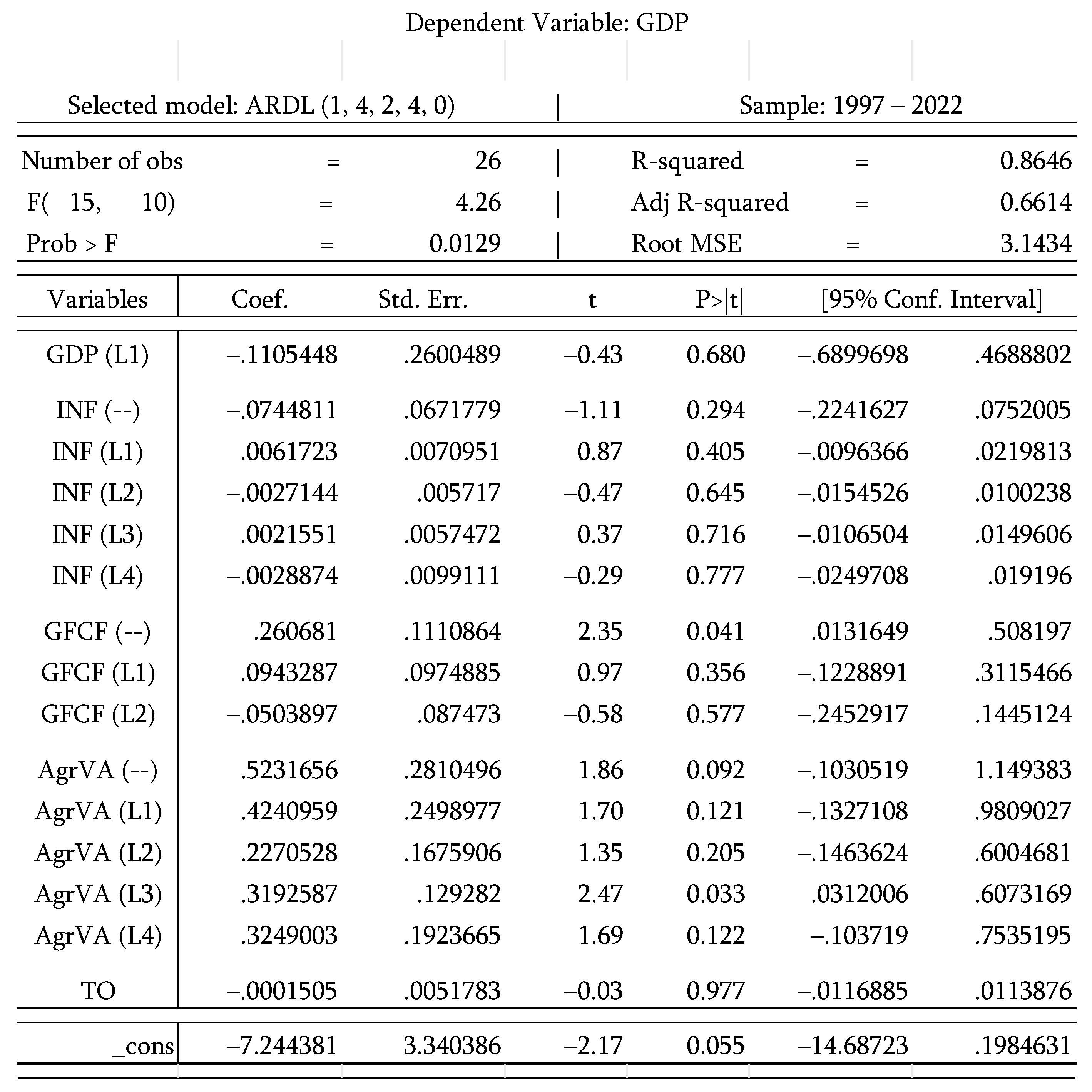
Figure 8.
Short run dynamics and error correction model resultsSource: Author’s computation using STATA 14.2.
Figure 8.
Short run dynamics and error correction model resultsSource: Author’s computation using STATA 14.2.
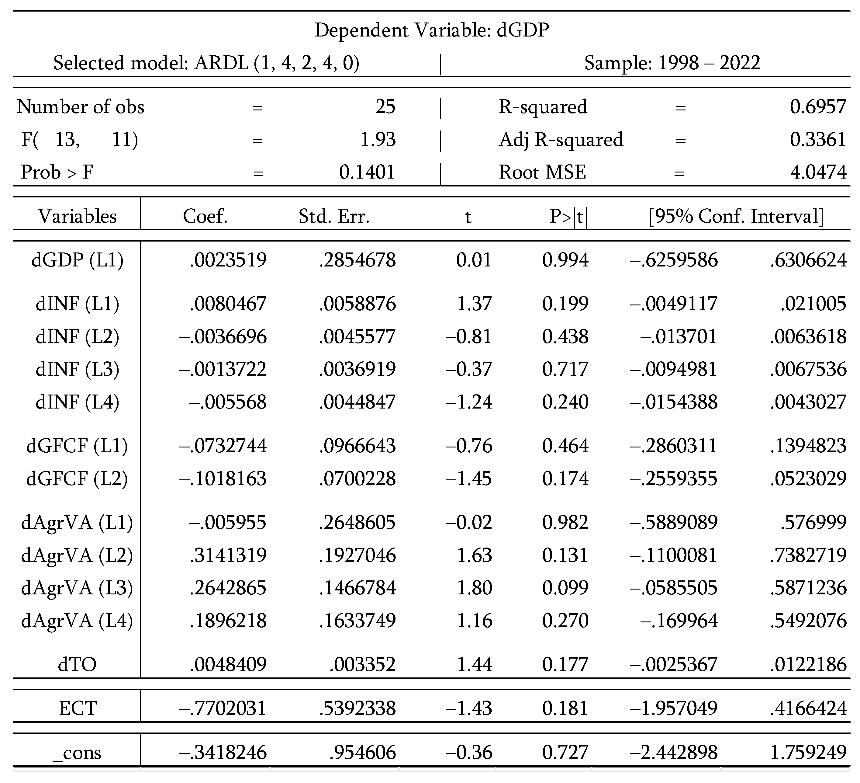
Figure 9.
Normality testSource: Author’s computation using STATA 14.2.
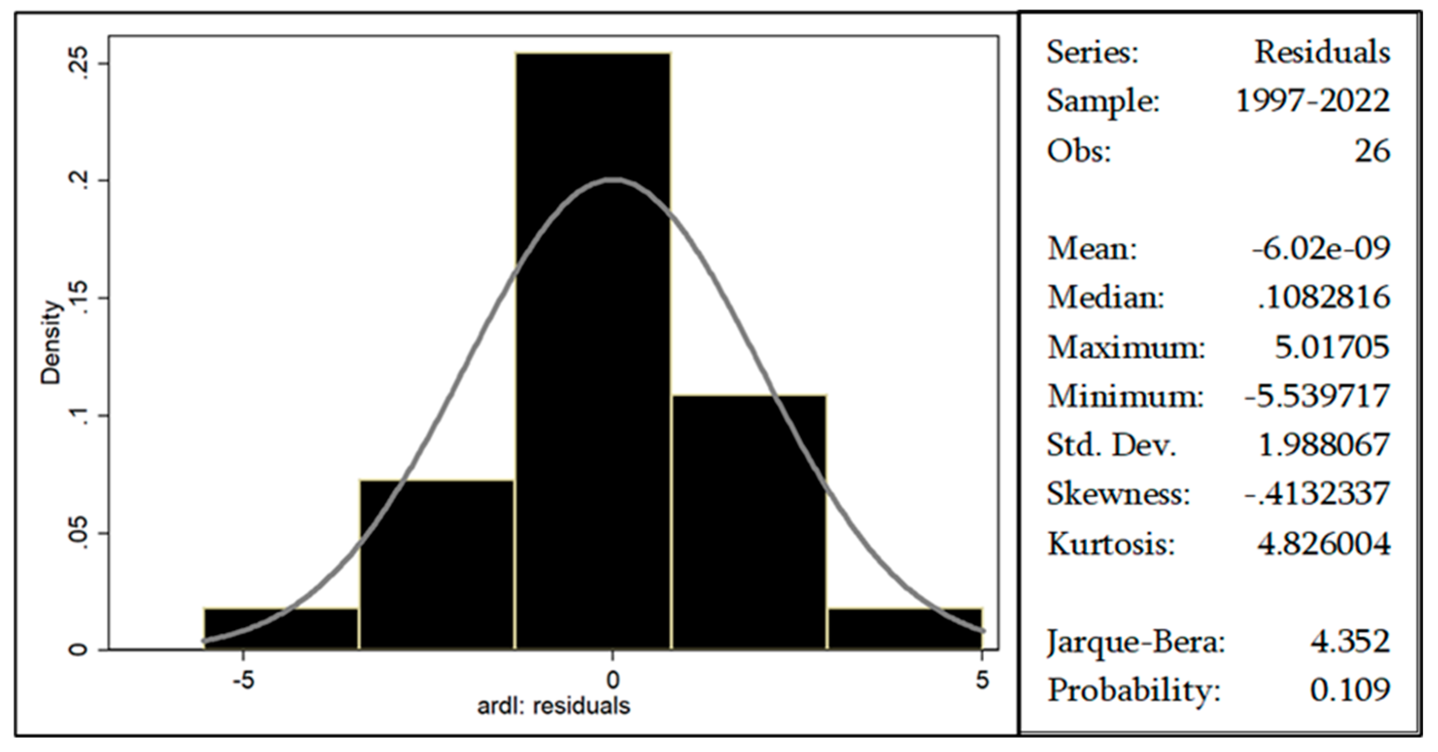
Figure 10.
VIF resultsSource: Author’s computation using STATA 14.2.
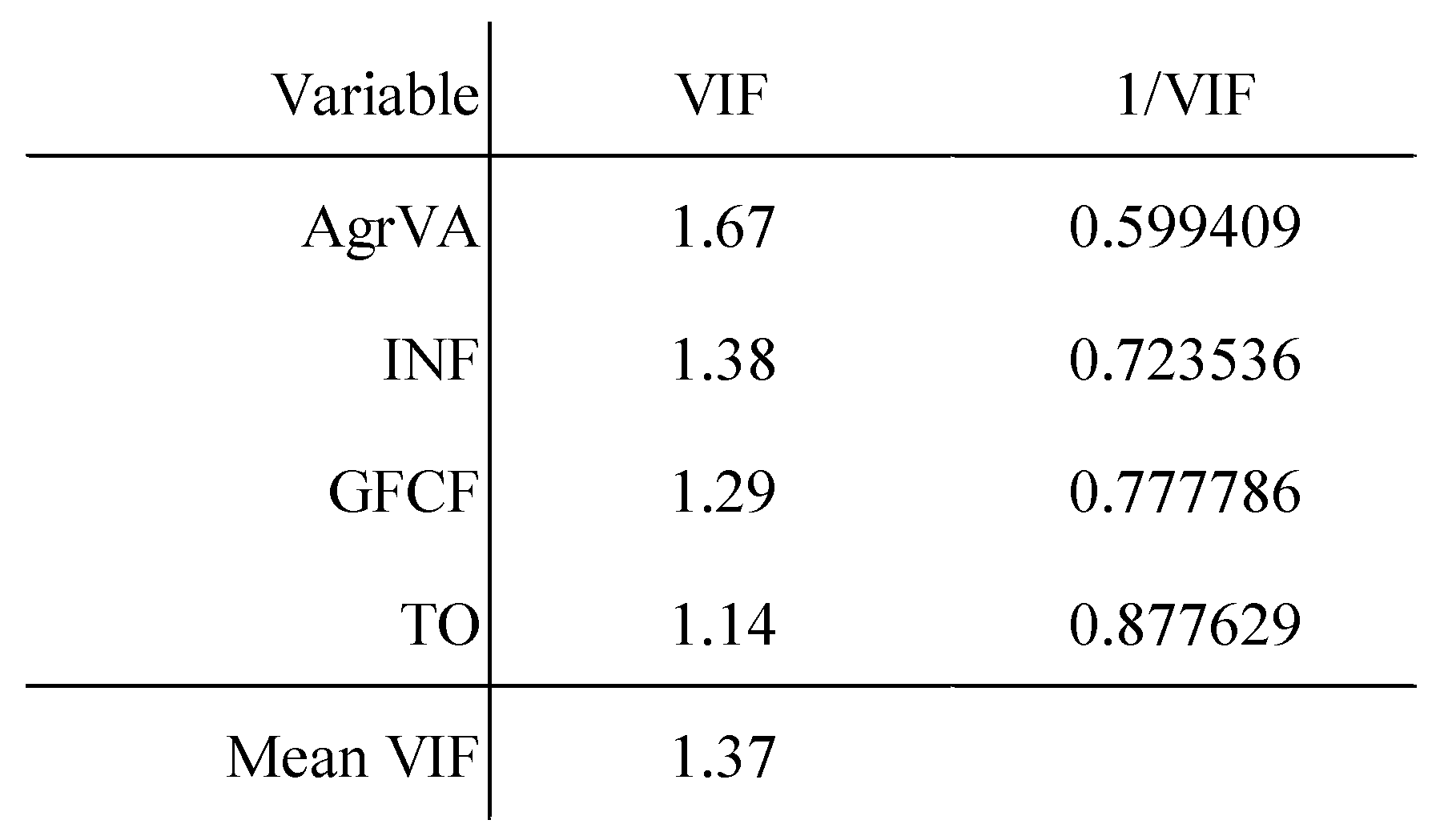
Figure 11.
Breusch-Godfrey test for autocorrelation. Source: Author’s computation using STATA 14.2.

Disclaimer/Publisher’s Note: The statements, opinions and data contained in all publications are solely those of the individual author(s) and contributor(s) and not of MDPI and/or the editor(s). MDPI and/or the editor(s) disclaim responsibility for any injury to people or property resulting from any ideas, methods, instructions or products referred to in the content. |
© 2024 by the authors. Licensee MDPI, Basel, Switzerland. This article is an open access article distributed under the terms and conditions of the Creative Commons Attribution (CC BY) license (http://creativecommons.org/licenses/by/4.0/).
Copyright: This open access article is published under a Creative Commons CC BY 4.0 license, which permit the free download, distribution, and reuse, provided that the author and preprint are cited in any reuse.


