As a classic topic in physics and mathematics, the research significance of the fastest motion lies not only in its theoretical exploration, but also in its broad practical application prospects. In fields such as geology and civil engineering, the problem of seeking the shortest time path is ubiquitous, and the steepest descent line problem provides an ideal theoretical model to explore these issues, and promotes our in-depth understanding of physical laws, stimulating our innovative thinking in fields such as geophysics and geological engineering.
The Earth tunnel problem, as one of theearliest derived models of thefastest motion problem, has been discussed in multiple studies [
1,
2,
3,
4,
5,
6,
7,
8]. Inhistory, research on the steepest descent line can be traced back to the 17th century, when mathematicians such as John Bernoulli proposed the famous steepest descent line problem in 1696, which was solved by mathematicians such as Newton and Leibniz. The solution to this problem not only promoted the development of variational calculus, but also laid the foundation for the proposal of the principle of minimum action in modern physics [
9].
Many literary and film works have also put forward their corresponding ideas. For example, Jules Verne's famousscience fiction work "Journey to the Center of the Earth" envisioned a hypothetical tunnel through the center of the Earth, running through both ends of the earth - people could pass through the tunnel and enjoy the fantastic scenery of the center of the Earth along the way; The games "Total Recall" and "Earth Cannon" "fulfilled Jules Verne's dream. This idea sparked extensive discussions on the issue of Earth tunnels, indirectly advancing research in related fields of physics, mathematics, and engineering.
However, so far the discussions have been limitedto the case wherethe tunnel shape is set to a straight line. Under this condition, a considerable number of studies [
1,
2,
3,
4,
5,
6,
7,
8] have established linear models, similar to those described in
Section 1, which conclude that when an object moves within an Earth tunnel connected by a chord line between two points on the Earth's surface, it undergoes harmonic motion. After finally substituting the relevant constants, the time required for the particle to move through a string connecting two points on the Earth's surface in an Earth tunnel is 42 minutes (ideally). The corresponding derivation process will not be repeated here.
So, if the earth tunnel between any twopoints on the surface of the earth is not limited in shape (i.e. a curve), would the travel time still be 42 minutes? In this article, the author will take this as a starting point and use Python visualization tools to clarify the analytical curve that needs to be followed and the relevant properties of the curve to open the fastest tunnel (of any shape) between any two points on the Earth's surface.
1. Model Establishment
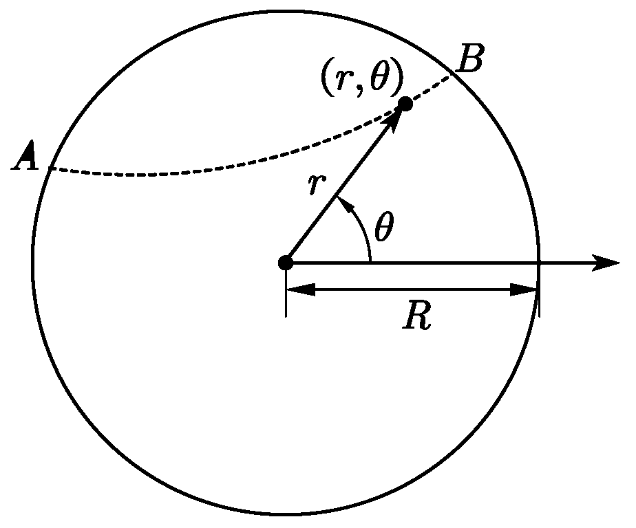
To solve the problem of curved earth tunnels, we first establish a model : assume that the earth is a uniform sphere with a radius of
R, a mass of
M, and a density of
ρ, then dig a (curved) tunnel of unlimited shape, regard any object in the tunnel as a mass point
m,
r is the distance between the mass point and the center of the earth, and establish a polar coordinate system with the center of the earth as the origin (as shown in
Figure 1). Ignore the centrifugal inertia of the earth's rotation, the Coriolis force, the size of the tunnel, the friction in the tunnel, etc., and discuss the movement of the mass point under the condition of only considering the action of universal gravitation.
2. Python Visualization Toolkit Analysis Modeling
2.1. Theoretical Modeling Process
According to Gauss's theorem, take any point (
r,
θ) inside the earth, then the gravity of the particle at that point points to the center of the sphere, and the magnitude is
Let
, assuming that the infinite distance outside the earth is the potential energy zero point, then the gravitational potential energy of a point (
r,
θ) inside the earth is:
Then, the energy conservation equation for the process of moving from a point on the earth's surface to a point inside the earth (
r0 ,
θ0) is listed as follows:
At the same time, according to the representation of velocity in polar coordinate system
the time
T required to travel from one point
A on the Earth's surface to another point
B on the Earth's surface.
To find out where the minimum value of
T is obtained, let
(where
), that is, to solve the minimum point (extreme point) of
f(
r). According to the Euler-Lagrange equation, if the function
T is required to obtain an extreme value, the function
f (
r) needs to satisfy the equation
To solve the differential equation more simply, we can use
to transform it into
Assuming that θ0 is the direction angle of the particle at the initial moment, then solving the transformed differential equation, we can finally obtain the analytical expression of the fastest descent line inside the earth in the polar coordinate system:
① ()
② (, are the endpoint values of the fastest curve )
Due to the domain of the inverse sine function, the premise for the analytical expression ① to be meaningful is
2.2. Python Visualization Code
2.2.1. Visual Code Design Ideas
(1) Function thetar
This function is used to calculate a certain θ under a certain r and the angle value θ 0 of the direction where the particle is located at the initial moment according to the analytical formula of the fastest curve ①. The input parameters are r, R, C and θ0 are calculated and output in two cases:
①At that time,
② Otherwise, still according to the calculation
(2) Function plot_q
This function is used to draw the fastest curve when C is a specific value. The thetar function needs to be called to calculate the coordinates of each point required to draw the graph.
(3) Main program
Set R (for the convenience of drawing, set R to 1) and the angle value θ 0 of the direction where the particle is located at the initial moment, and call the function plot_q to draw the fastest curve under different C values.
For each C value, the plot_q function is called to draw the corresponding curve and set the legend. Finally, plt.show() is used to display a series of images of the fastest curves under different C values.
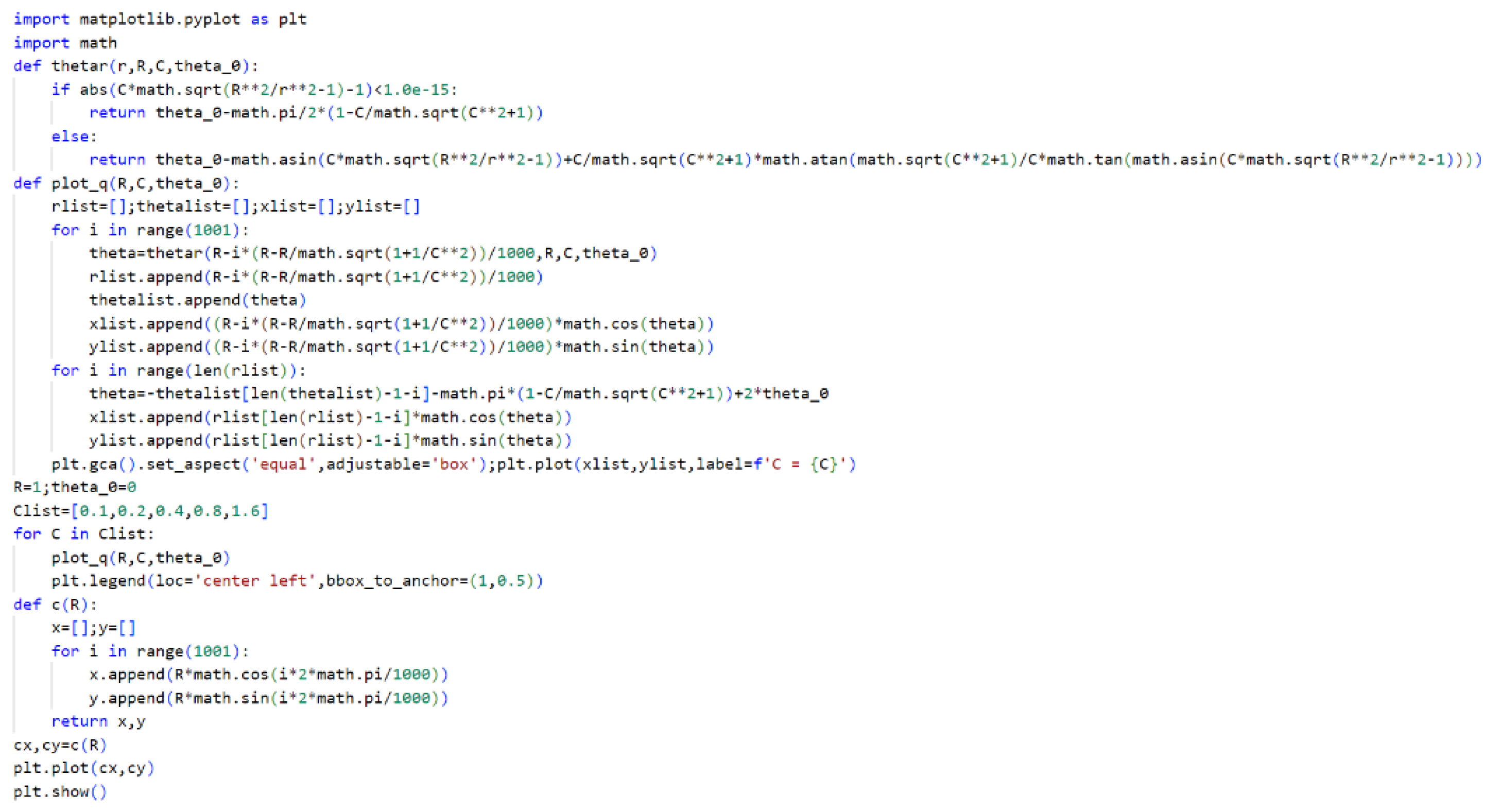
2.2.2. Visualization Code and Visualization Results
According to the design ideas described in
Section 2.2.1, the visualization code is shown above (which is also shown in
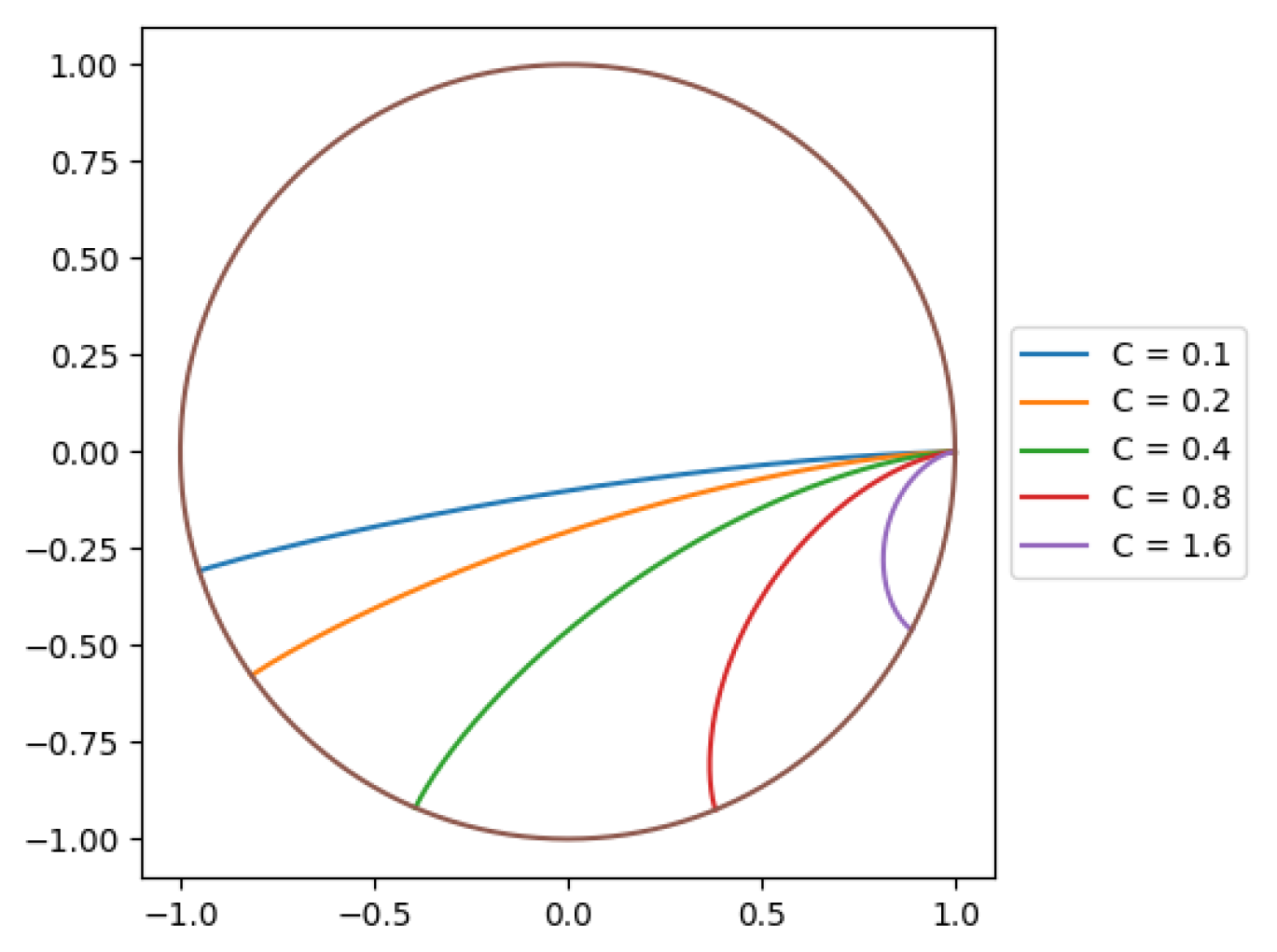
Figure 2), and the visualization result is shown in
Figure 3.
import matplotlib.pyplot as plt
import math
def thetar(r,R,C,theta_0):
if abs(C*math.sqrt(R**2/r**2-1)-1)<1.0e-15:
return theta_0-math.pi/2*(1-C/math.sqrt(C**2+1))
else:
return theta_0-math.asin(C*math.sqrt(R**2/r**2-1))+C/math.sqrt(C**2+1)*math.atan(math.sqrt(C**2+1)/C*math.tan(math.asin(C*math.sqrt(R**2/r**2-1))))
def plot_q(R,C,theta_0):
rlist=[];thetalist=[];xlist=[];ylist=[]
for i in range(1001):
theta=thetar(R-i*(R-R/math.sqrt(1+1/C**2))/1000,R,C,theta_0)
rlist.append(R-i*(R-R/math.sqrt(1+1/C**2))/1000)
thetalist.append(theta)
xlist.append((R-i*(R-R/math.sqrt(1+1/C**2))/1000)*math.cos(theta))
ylist.append((R-i*(R-R/math.sqrt(1+1/C**2))/1000)*math.sin(theta))
for i in range(len(rlist)):
theta=-thetalist[len(thetalist)-1-i]-math.pi*(1-C/math.sqrt(C**2+1))+2*theta_0
xlist.append(rlist[len(rlist)-1-i]*math.cos(theta))
ylist.append(rlist[len(rlist)-1-i]*math.sin(theta))
plt.gca().set_aspect('equal',adjustable='box');plt.plot(xlist,ylist,label=f'C = {C}')
R=1;theta_0=0
Clist=[0.1,0.2,0.4,0.8,1.6]
for C in Clist:
plot_q(R,C,theta_0)
plt.legend(loc='center left',bbox_to_anchor=(1,0.5))
def c(R):
x=[];y=[]
for i in range(1001):
x.append(R*math.cos(i*2*math.pi/1000))
y.append(R*math.sin(i*2*math.pi/1000))
return x,y
cx,cy=c(R)
plt.plot(cx,cy)
plt.show()
Figure 2.
Python Visualization Code.
Figure 2.
Python Visualization Code.
Figure 3.
Python Visualization Results.
Figure 3.
Python Visualization Results.
3. Python Visualization Result Analysis
As can be seen from
Figure 3, the smaller
C is, the longer the distance the particle moves inside the earth, and the closer the steepest descent line is to a straight line. When
θ0 is fixed, given an integral constant
C, there is only one steepest descent line. Here we can calculate the time required for the particle to move from the initial point to the end point along this steepest descent line:
Substituting
into the above formula, we can get
Substituting the upper and lower limits of the integral at points A and B, we get
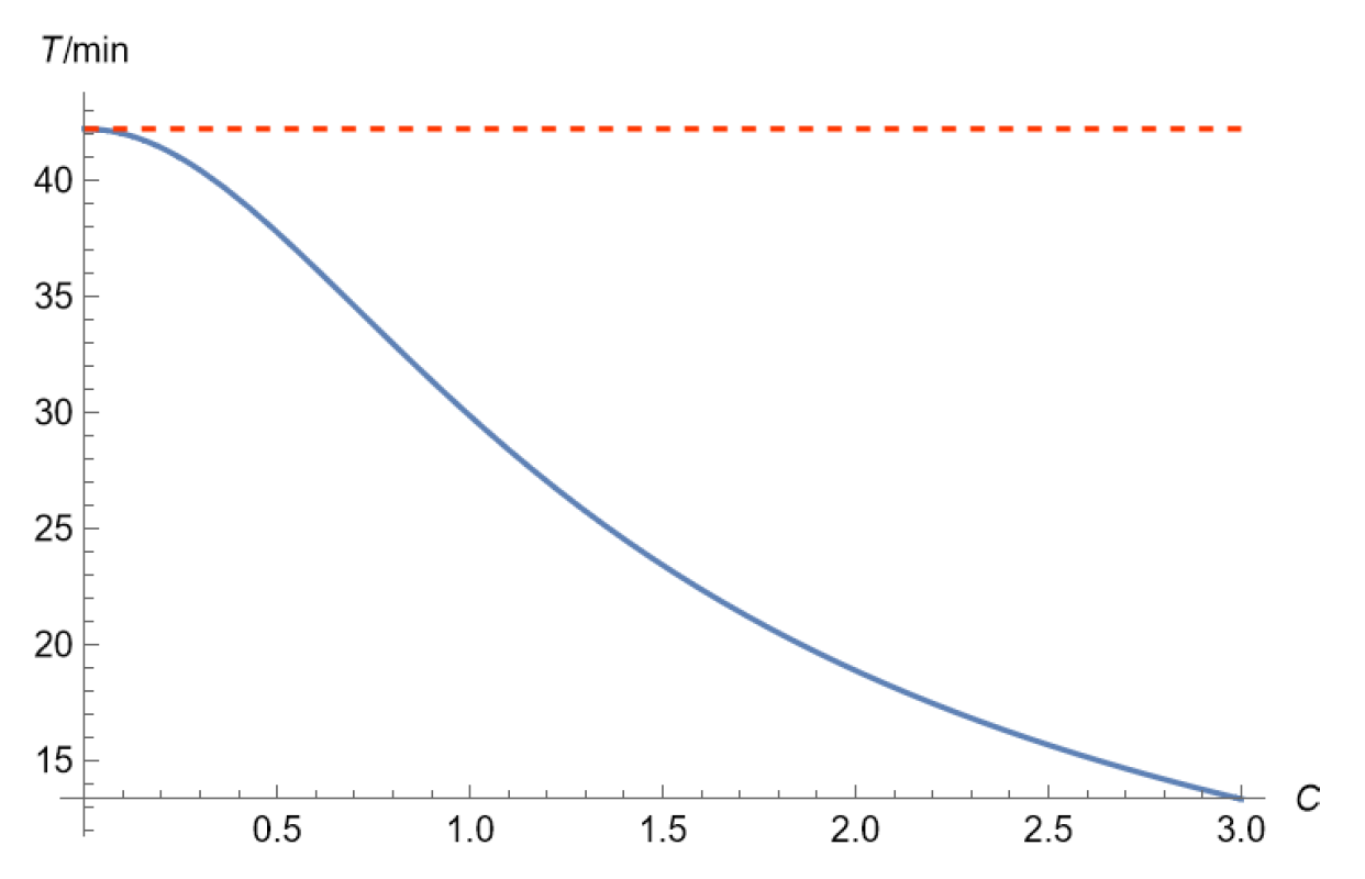
Using the Python visualization toolkit, write code to plotTagainst C, showing therelationship between the corresponding C values of particles in different tunnel curves and the time T required to travel from point A through the Earth's interior to point B (as shown in
Figure 4, the dashed line represents the reference value of 42 minutes in the case of degradation to a straight line). At this point, substitute the real data with a value of 1.24×10
-3 rad/s.
Next, let's consider the actual physical meaning of the integral constant
C. Assume that the angular coordinate of the particle leaving the earth tunnel is
θ ex , then from the analytical expression of the fastest curve in 2.1, we know that
Assume that the difference in angular coordinates of the particle entering and exiting the earth tunnel is
θ ab = θ 0 - θ ex (
θ ab ∈[0,
π ]), then the magnitude of the integral constant
C is
This formula gives the physical meaning of the integration constant.
Substituting the above formula back
into the equation, we get
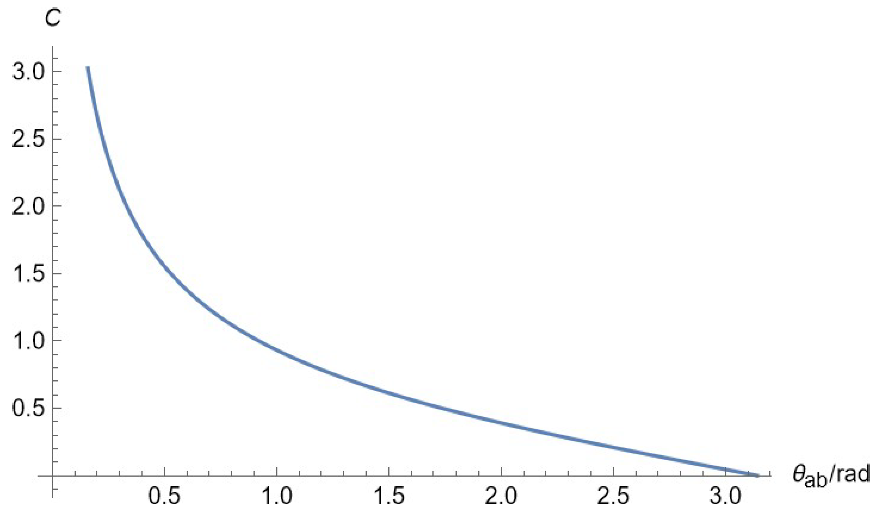
Similarly, toclearly understand the relationship between the angular coordinate difference θ ab and the corresponding dimensionless integration constant C, as well as the required time T, we use Python visualization toolkit,write code to plot T and C against θ
ab, as shown in
Figure 5 and
Figure 6.
When
θ ab =
π, the problem is reduced to the case of digging a straight earth tunnel inside the earth (as shown by the dashed line in
Figure 6). From the above equation combined with
Figure 4 and
Figure 6, it can be seen from the above formula that digging a straight earth tunnel inside the earth does not actually make the time taken by the particle from point
A to point
B through the earth's interior the shortest, and in general, the straight tunnel is the path that takes the longest time.
4. Conclusion and Expectation
Python's strength lies in its ability to handle large datasets and to integrate with other data analysis tools. However, it requires a certain level of programming knowledge and can be overkill for simple visualization tasks,while students and teachers possibly do not have the knowledge that supports the visualization process in Python.Also,visualization results generated using Python can sometimes appear less smooth when the number of manually controlled sampling points is insufficient. This limitation arises because the quality and smoothness of a visualization are highly dependent on the density and distribution of the data points. With fewer sampling points, the visual representation may not accurately capture the underlying patterns or trends in the data. Additionally, the lack of sufficient sampling points can lead to jagged or discontinuous lines in plots, which can be misleading or difficult to interpret,which might confuse the thinking of students. Furthermore, this issue can also affect the ability to interact with the visualization in real-time. Real-time interaction typically requires a dynamic and responsive system that can update the visualization as the user manipulates the data or explores different aspects of the visualization. When the data is sparse or the sampling points are not optimally distributed, the system may struggle to provide a seamless and responsive user experience. This can result in delays or inaccuracies in the visualization updates, which can hinder the user's ability to explore the data effectively and make informed decisions based on the visual insights.
All in all,in this paper, we explored the problem of the fastest motion of an object in a curved earth tunnel by building a mathematical model and using the Python visualization toolkit. Through in-depth analysis of the model, we not only derived the analytical expression of the brachistocentric curve, but also revealed the physical meaning of the integral constant C, which is related to the difference in the angular coordinates of the particle entering and exiting the earth tunnel. Our results show that, contrary to intuition, a straight tunnel is not always the fastest path, and a curved tunnel can significantly reduce the time it takes for an object to traverse the earth in most cases. In addition, this research method that combines mathematical software and physical models can help students better expand their thinking about physical models. With the assistance of software tools, even complex extended physical problems can become easy to understand and master, which is of great significance for improving teaching effectiveness and students' learning efficiency.
References
- Cui Shengzhe, Jia Weiyao, Zhu Jianhui. Using the shell theorem to solve the earth tunnel problem[J]. Discussion on Physics Teaching, 2024, 42(03):73-76.
- Luo Shuyuan, Hu Nan, Cai Liudong. Analysis and discussion of several motion cycles[J]. Bulletin of Physics, 2024, (02): 148-150.
- Ouyang Zhihui, Chen Haixiu. 42 minutes in the earth tunnel[J]. Discussion on Physics Teaching, 2023, 41(03): 63-64.
- Wu Daizong, Liu Yuying. Movement of objects in earth tunnels[J]. Physics and Engineering, 2020, 30(01): 73-79.
- Miao Lihua, Han Dejun. The answer is 42 - there are many questions but only one answer [J]. Physics Teacher, 2005, (10): 36-37.
- Liang Zhiqiang. Tunnel through the earth[J]. Journal of Taian Teachers College, 1998, (06): 35-37.
- Wang Changming. Motion of a free particle in a smooth tunnel in the earth[J]. University Physics, 1990, (05): 4-6.
- Huang Shichu. Discussion on the motion of objects in a straight tunnel through the earth[J]. Journal of Anhui Institute of Technology, 1987, (Z1): 139-148.
- Ding Guang-Tao. Damped brachistochrone problem and the relation between constraint and theorem of motion[J]. Acta Physica Sinica, 2014, 63(7): 070201-070201. [CrossRef]
|
Disclaimer/Publisher’s Note: The statements, opinions and data contained in all publications are solely those of the individual author(s) and contributor(s) and not of MDPI and/or the editor(s). MDPI and/or the editor(s) disclaim responsibility for any injury to people or property resulting from any ideas, methods, instructions or products referred to in the content. |
© 2024 by the authors. Licensee MDPI, Basel, Switzerland. This article is an open access article distributed under the terms and conditions of the Creative Commons Attribution (CC BY) license (http://creativecommons.org/licenses/by/4.0/).