Submitted:
09 October 2024
Posted:
18 October 2024
You are already at the latest version
Abstract
In underwater clustering and benchmark networks, nodes need to reduce the rate and energy consumption of acoustic communication while ensuring synchronization accuracy. In large-scale networks, the improvement of the efficiency of existing network time synchronization often relies on optimization of topological structures, and the improvement in efficiency within local areas is limited. This paper proposes a method to synchronize underwater time using the probability graph model. The method utilizes the positional and motion status information of sensor networks to construct a factor graph model for distributed network synchronization. By simplifying the marginal probability density function of the system clock difference, it can quickly calculate the clock difference parameters of nodes, thereby effectively improving the synchronization efficiency. Experimental results show that the method can complete global time synchronization within a cycle while achieving a clock difference correction accuracy higher than seconds, significantly optimizing the synchronization period and efficiency, and reducing the energy consumption of acoustic communication.
Keywords:
Underwater Network Time Synchronization
; Factor Graph Model
; Distributed Networking
1. Introduction
Network time synchronization refers to the process of synchronizing time across nodes in a network using network protocols. For surface time synchronization, it usually combines the standard time reference provided by GNSS and propagates time information through the network. Network time synchronization is widely used in data centers, distributed systems, communication networks, and other scenarios requiring time synchronization. It focuses on achieving time synchronization through network protocols in distributed computing environments, involving clock hierarchical architecture and adaptation to different network topologies.
The Network Time Protocol (NTP) is the most widely used network time protocol. It uses a hierarchical structure to organize time servers. Research in recent years has focused mainly on improving NTP security and resilience to interference, such as the work of Burbank et al. [1]. The Precision Time Protocol (PTP) is a typical centralized network protocol in which one device in the network is selected as the Master Clock and other devices act as slave Clocks, obtaining time from the Master Clock. Researchers have been working to improve the accuracy of PTP synchronization using hardware timestamps and clock filtering algorithms [2].
Network time synchronization methods are also widely applied in cloud computing and distributed databases. Research focuses on achieving reliable time synchronization in high-latency and unstable network environments [3]. It includes FTSP [4], RBS [5], and Delay Measurement et al. Time Synchronization for Wireless Sensor Networks (DMTS) [6]. The network structures of these protocols can be referenced for underwater time synchronization, but the synchronization process is not applicable due to the large propagation delay underwater. Compared to surface applications, underwater sensor nodes are usually powered by batteries, and the limited power supply severely restricts the computational and communication capabilities of the sensor nodes. Therefore, the structure of underwater networks is relatively simple and can generally be divided into three types based on network methods: centralized, distributed, and multi-hop, as shown in Figure 1.
In 2003, Ganeriwal et al. [7] proposed the Time Synchronization Protocol for Sensor Networks (TPSN) based on centralized network structures. Similarly to the NTP protocol, it classifies network nodes hierarchically and assigns each node a level number. The root node, which serves as the clock source for the entire network, is designated level 0, while other nodes synchronize with a node from the previous level, ultimately synchronizing all nodes with the root node. However, this method cannot prevent network paralysis caused by root node failure and is unsuitable for networks with highly mobile nodes.
In 2017, Wang Shuo et al. [8] proposed an energy-optimal clustering method for underwater sensor networks, dividing time synchronization into inter and intra cluster synchronization [9], and calculating the optimal number of clusters by solving mathematical expectations. This method is not suitable for highly mobile networks, as significant changes in network topology require recalculation of the optimal number of clusters and re-clustering.
In 2020, Kong Weiquan et al. [10] proposed a dual cluster head time synchronization algorithm for underwater sensor networks based on clustering. By selecting two nodes as primary and secondary cluster heads, it improved the network robustness and improved the accuracy and efficiency of time synchronization. It also considered the impact of node mobility on synchronization accuracy, reducing estimation errors to some extent by introducing advanced node mobility models. However, given the complexity of the mobility of the underwater network, this method is difficult to implement.
For time synchronization in mobile networks, the accuracy of synchronization can be improved by providing the assistance of dynamic nodes [11,12,13], or by employing more accurate models of network node mobility [14,15,16,17]. However, despite the benefits of clustering nodes in reducing the messaging overhead for time synchronization in underwater sensor networks and improving the overall network synchronization accuracy, there are still deficiencies when it comes to dealing with mobile nodes. Furthermore, in small areas, the efficiency gains from centralized networking synchronization are not significant.
Multi-hop networking offers higher robustness compared to clustering models. For example, Sun C et al. [18] proposed Multi-hop Time Synchronization for Underwater Acoustic Networks (MSUAN) in 2012, emphasizing the reduction of synchronization errors through multilevel timestamp exchanges. Subsequently, Wen J et al. [19] proposed an Improved Multi-Hop Time Synchronization for Underwater Acoustic Networks (IMSUAN) in 2013, improving synchronization accuracy by establishing a time synchronization tree and optimizing node listening mechanisms, and using global bias thresholds to filter out inaccurate timestamps.
However, both clustering models and multi-hop network models are more suitable for large-scale network nodes, i.e., when node communication distances cannot cover the entire network. In small-scale networks (where node communication distances can cover the network), both models are not different from centralized networks and are limited by central nodes. Moreover, the actual synchronization algorithms do not differ from the time synchronization algorithms between two points(such as DE-Sync [22]) and do not fully utilize the network information. In most cases, underwater sensor nodes, whether mobile submersibles or stationary underwater beacons, have some ability to acquire location information. Integrating location information with sound velocity information can greatly simplify the time-synchronization process. Higher location information accuracy can lead to higher time synchronization accuracy. However, the computational complexity brought about by multiinformation fusion and the communication pressure from distributed network structures increase the energy consumption burden of underwater networks. How to achieve rapid time synchronization in underwater networks while maintaining a certain level of energy consumption is the research objective of this paper.
To address these issues, this paper proposes a time synchronization method based on a probability graph model for underwater networks. This method solves the marginal probability density function of the system clock offset parameters and performs binary simplification to quickly calculate the clock offset parameters of various sensors within the local network, achieving dynamic time synchronization in distributed networks. Compared to conventional network time synchronization methods, the probability graph model-based time synchronization method employs distributed networking, reducing dependence on central nodes and improving network robustness. This method improves multi-user protocols, integrates location and sound velocity information, significantly enhancing synchronization efficiency, and reduces computational requirements for nodes through binary simplification of the algorithm.
2. Application Scenarios
The underwater network time synchronization methods discussed in this paper is applied in a scenario where sensor networks periodically synchronize their time reference. When node A receives a signal from node B, it records the reception time and its own position Similarly, each synchronization round can obtain time values: , , , , , and node positions: , , , which constitute one cycle of time synchronization for the sensor network. In addition,the network must measure the average sound velocity C in the water layer where it is located. The above describes a section of a research paper.
Figure 2.
Schematic diagram of underwater network time synchronization scenario.
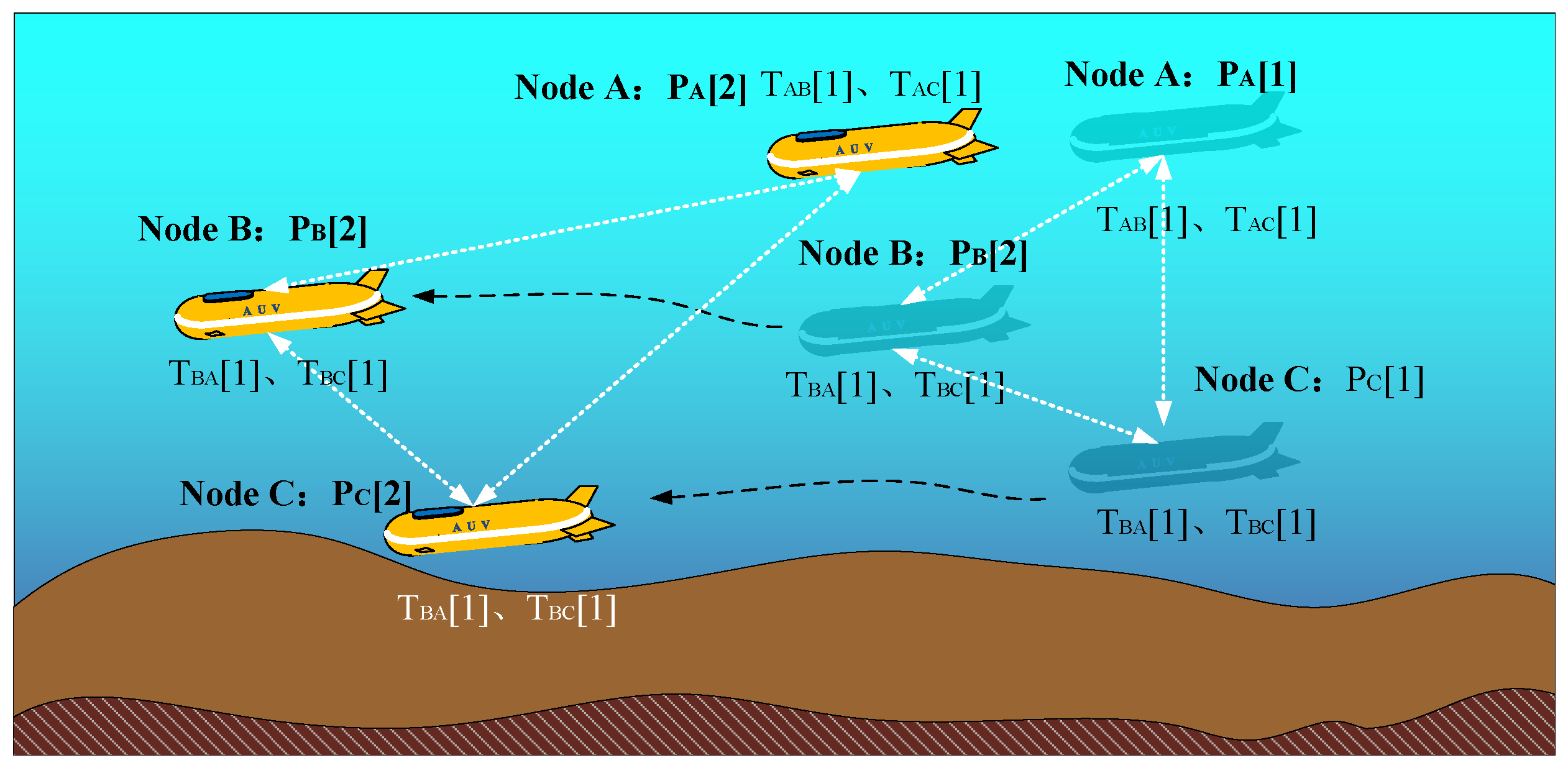

Table 1.
Measurement parameters table for network time synchronization Methods.
| Parameters | Explanations |
|---|---|
| The timestamp at which node i receives the synchronization message from node j during the interaction | |
| The position of node in at the interaction | |
| C | The average sound velocity in the water layer where the network is located |
1 Tables may have a footer.
3. Principles of Underwater Network Time Synchronization Methods
To simplify the existing network time synchronization protocol and increase synchronization efficiency, additional information is clearly needed as support. Information fusion would increase the computational burden on nodes, while reducing the central node’s constraints on the network. Adopting a distributed network would require further network communication resources. This paper attempts to utilize factor graph models to simplify the entire network time synchronization process, thereby reducing the communication and computational demands of network synchronization.
3.1. Network Configuration Methods
The probabilistic graph method adopts a distributed hierarchical network approach. Taking the underwater network in Figure 3 as an example (it is generally assumed that the communication range of the cluster head nodes is greater than that of ordinary nodes), the network can be divided into 6 networks based on the communication range of the nodes. Each network forms its own distributed network, while the five cluster head nodes form a larger distributed network. In this case, each node is not a central node for its local network, and the cluster head nodes only serve as time-reference standards for the local network rather than initiators of all synchronization activities. When a cluster head node fails, the distributed network can use the time of any node within the network as a reference, achieving unification of the local network.
The scope of hierarchical distributed networking is limited by the communication range of the cluster head nodes. For larger-scale networking, the communication distance of the cluster head nodes cannot cover the entire underwater acoustic network, which requires multi-hop-assisted networking. As shown in Figure 4, distributed networking is used within clusters, while multi-hop communication is employed between clusters.
3.2. Message Passing Scheme
Cluster-based networking and multihop networking can significantly improve synchronization efficiency in large-scale networks. However, these improvements are primarily based on optimizations in topological structure and offer no enhancement in local areas (within the communication coverage of a single node) compared to inter-platform time-synchronization methods.
The intracluster information transmission scheme (multiuser protocol) is shown in Figure 5. It is evident that existing network time-synchronization methods, while needing to consider information differentiation among multiple users, are fundamentally not different from one-way or two-way time-synchronization methods. They do not fully utilize the additional information available in sensor networks, thus missing the opportunity to simplify the time-synchronization process in underwater sensor networks.
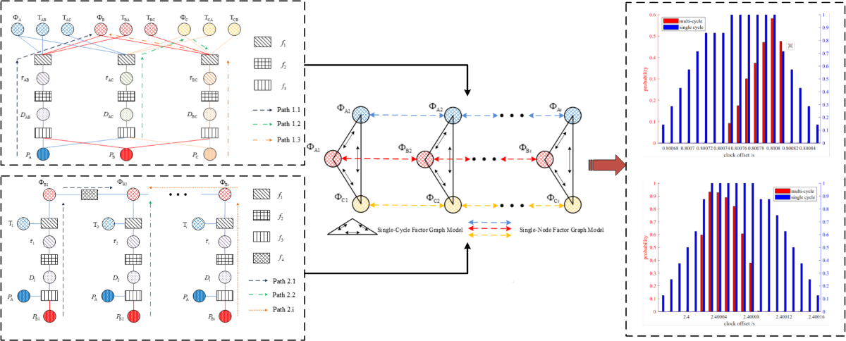
The probability graph method for time synchronization, as illustrated in Figure 6, differs from previously used methods that require multiple interaction cycles to complete a single time synchronization. In contrast, the probability graph method can complete a time synchronization in each interaction cycle (). In addition, multiple sets of interactions can further improve the accuracy of the synchronization.
3.3. Factor Graph Models
3.3.1. Single-Group Interaction Time Synchronization Model
This model is generally applied to underwater sensor networks (clusters, reference networks, etc.) that require high refresh rates. In this scenario, the reference points have certain initial position values and the unification of the time reference can be achieved through relative ranging. Due to the ability to achieve real-time time reference alignment, there is no need to correct clock drift.
The fusion parameters include reference position information, reference clock offset, relative ranging information, time delay difference measurement information, and relative ranging signal reception moments. At this point, the global function is represented as:
In 1, represents the set of clock offset for each reference beacon, denotes the set of all measurement signal reception times, represents the set of time delay difference measurements, is the set of range measurements, and is the set of underwater reference positions.
Taking the inter-beacon ranging among three beacons A, B, and C (with A as the reference beacon, as an example, the factor graph model as shown in the Figure 7:
represents the reference among signal reception time, time delay and reference clock offset. represents the functional relationship between the information from the range and the time delay difference. represents the functional relationship between the information from the range and the reference position.
Let:
The expression of the edge function
The relationship between clock offset , reception time T, and measured delay is
represents the measurement error of time, which follows . The function can be expressed as:
The relationship between range information D and time delay is
represents the measurement error of the sound velocity; it follows that . Therefore, the function can be expressed as:
The relationship between the reference position information P and the range information D :
represents the positional error, which can be represented by a distribution of . Then , , respectively, denote the horizontal and vertical coordinates of the reference point and represent the horizontal and vertical components of the distance .
Let then u follows a noncentral chi-square distribution with 2 degrees of freedom:
, the function can be expressed as
By analogy to the derivation of the reference B, the marginal probability density function for the clock offset of reference C can be obtained similarly.
3.3.2. Comprehensive Time Synchronization Model for Multiple Group Interactions
Compared to single-cycle interactions, a factor graph model that integrates information from multiple interactions can achieve higher accuracy of clock offset estimation. Taking multiple interactions between reference A and mobile platform B as an example, the single-node time synchronization factor graph model is as follows:
Figure 8.
Factor graph model for single node underwater network time synchronization.
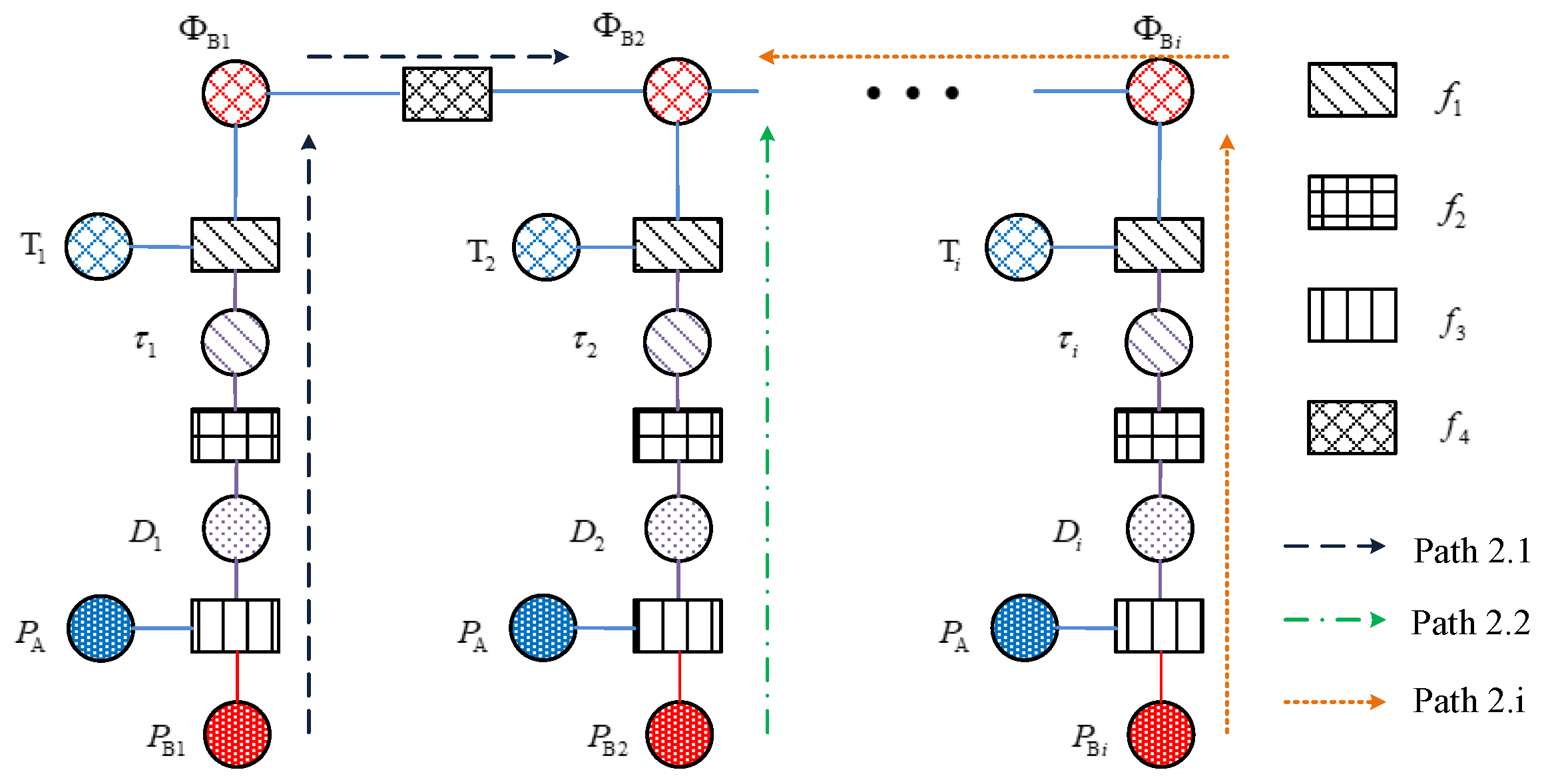
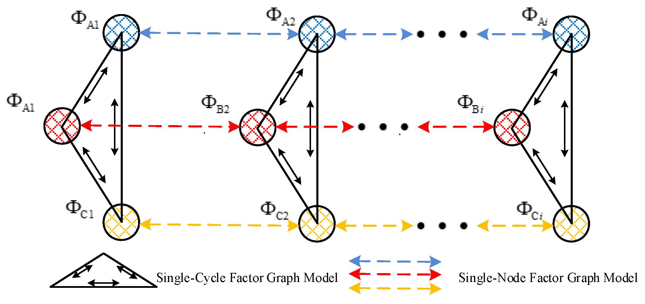
express the functional relationship between adjacent time interval clock offset. The multicycle interaction model is a combination of the single-cycle model and the single-node model.
Figure 9.
Factor graph model for multi-cycle underwater network time synchronization.
Let
n is the maximum number of interactions. Taking ’’ as an example, the expression for its marginal function is:
The relationship between the clock offset at time i (denoted as ) and the clock offset at time j (denoted as is:
Among them, represents the skew in clock frequency and represents the jitter error in the clock phase, which follows .
3.4. Binary Simplification
Under normal circumstances, the position, distance, delay, clock offset , and other information about the target to be estimated are distributed continuously, and the correlation functions between variables are also distributed continuously. Directly estimating the clock offset by calculating the expectation of the continuous distribution function has a high computational complexity. Therefore, the sampling concept is introduced to discretize the continuous distribution function. The most probable result of the clock offset distribution is divided into grids, each grid representing an estimated clock offset value. The final estimated result of the clock offset is obtained by weighted averaging of the estimated values for each grid. The main steps for calculating the weights are as follows. If the measured data set is known, fixed-interval scattered points can be used to represent the grid area . The weight of this grid area is represented by the value of the probability density function at the position . The calculation of the factor graph mainly focuses on the transmission and updating of messages. To reduce complexity, we adopt a binary mode for message transmission. The binary mode transforms the sum operations in the message transmission process into logical OR operations and product operations into logical AND operations, greatly reducing the computational load.
Based on binary mode, the probability density function of distance information can be simplified to
The probability density function of delay information can be simplified to
Under single-group interaction, the probability density function of node clock offset can be simplified to
The probability density function of clock offset between nodes under multiple interactions can be separately simplified to
represent the standard deviations of the respective probability density functions.The binary representation of message transmission is
3.5. Algorithm Process
This section focuses on the time synchronization scenario between underwater benchmarks. After establishing a factor graph model, the sum-product algorithm is employed to calculate the marginal probability function. Finally, to simplify the computational process, discretization and binary representation are adopted for the calculations.
The simplified algorithm flow is as follows:
Table 2.
Pseudocode of Single-Cycle Probability Graph Method
| Algorithm 1: Single-cycle probability graph time synchronization algorithm |
|---|
| Procedure Estimated clock offset( |
| Reference node A and n nodes to be synchronized |
| Sound velocity and reciprocal range observations |
| Position, speed of sound, time instant observed value accuracy |
| ) |
| Select any two points |
| Calculate the clock offset of node i at ,path 1.1 |
| Similarly |
| 4 For all , there exists a that satisfies 15 |
| 5 For all , there exists a that satisfies 16 |
| 6 For all , there exists a that satisfies 17 |
| Calculating the clock offset at node id when , Path 1.2 |
| Same as steps |
| Calculate the clock offset of node i in set , path 1.3 |
| For |
| Same as steps |
| Calculate the final clock offset of node i |
| Output |
Repeating for N cycles, the clock offset can be obtained for a single node, and by combining the single-node factor graph model, the estimated value of the comprehensive multicycle clock offset can be obtained.
Table 3.
Pseudocode of Multi-Cycle Probability Graph Method
| Algorithm 2: Comprehensive multi-cycle probability graph time synchronization algorithm |
|---|
| Procedure Estimated clock offset( |
| Multiple clock offset measurements for node i |
| //Single-cycle clock offset estimation accuracy |
| ) |
| Select the clock offset at time j for node i |
| Calculate the clock offset at time j for node i, following path 2.1 to end |
| 3 For all , there exists that satisfies the 19 |
| Calculate the final clock offset at time j |
| Output |
4. Field Experiments
4.1. Overview of the Experiment
On 3 April 2023, at 10:58 AM, an underwater cluster time synchronization experiment was conducted in the South China Sea at a depth of 3400 meters. The experiment involved the deployment and calibration of four seafloor beacon transponders, with a total duration of 3 hours.
Figure 10.
experimental site

The frequency band of the communication signal ranged from 2 to 4 kHz. The relative positions of the deployed beacons are shown in Figure 11 (Beacon J3 was excluded from subsequent data processing due to battery depletion and incomplete data collection).
The sound velocity profile was collected on April 3, 2023, at 19:10:09. The results of the acquisition of the sound velocity are shown in Figure 12.
The benchmark inter-interaction cycle is 20s, with J1, J2, and J4 having forwarding delays of 0s, 0.8s, and 2.4s respectively. The beacon clock source is an SA.45s rubidium clock model, with a cumulative drift of less than s over 135 hours. Therefore, it can be assumed that the clock offset remains constant during the experiment. Assuming that each beacon uses its transmission moment as the local clock’s 0 moment, the clock offset for each beacon are 0s, 0.8s, and 2.4s, respectively.
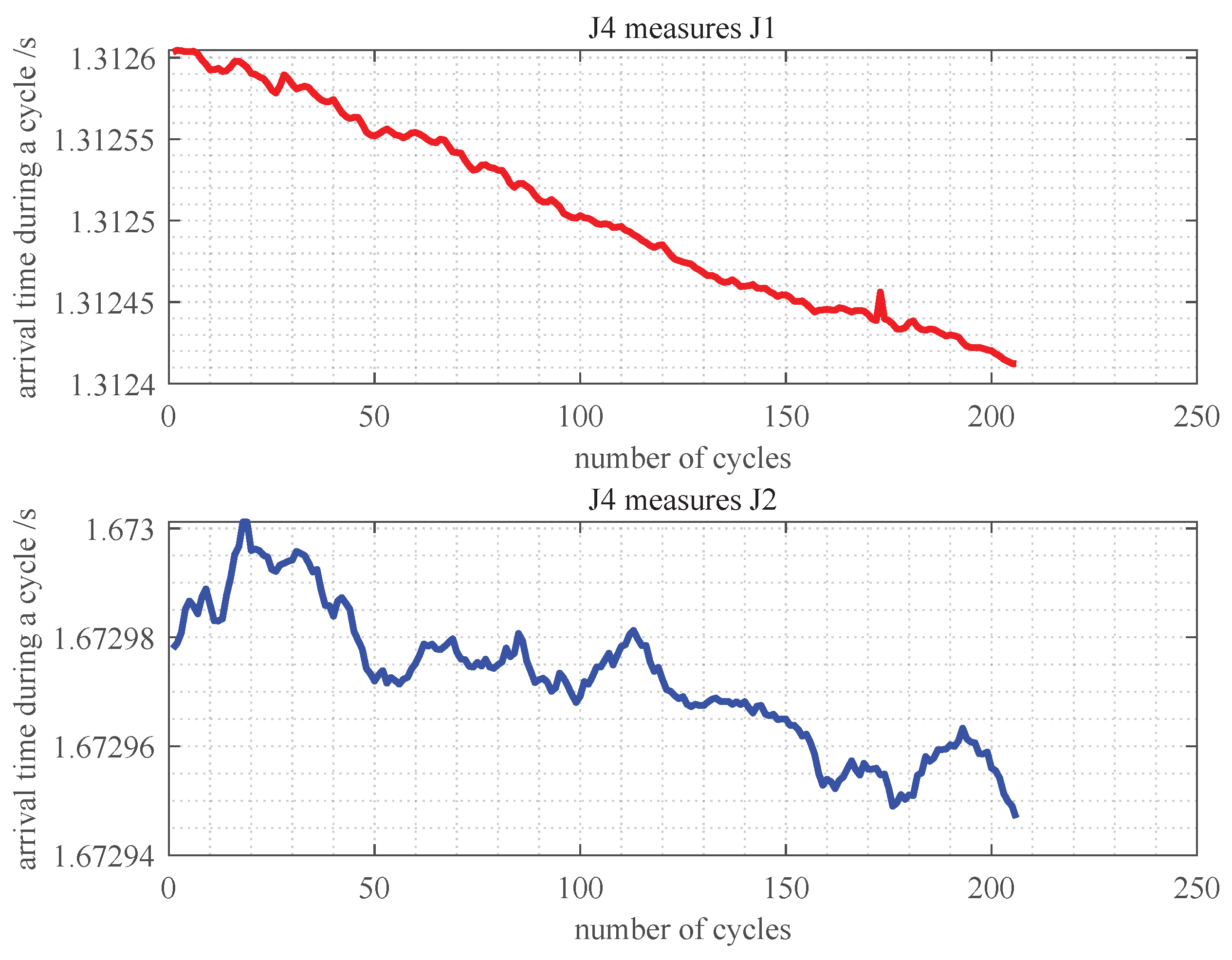
The experiment collected 206 cycles of intermeasurement signals with a 10 s cycle. Each beacon recorded the arrival times of the signals from other beacons, using its own transmission moment as a reference, as shown in Figure 13 to Figure 15. It can be seen that the fluctuation amplitude of the delay measurements is consistently below . This error is primarily due to variations in the velocity of the sound. This amplitude represents the upper limit of the accuracy of clock-offset measurement and serves as the main basis for setting the resolution in discrete calculations. Excessively high resolution would affect computation speed, while too low resolution would reduce synchronization accuracy. For these experimental data, the clock offset resolution was set to .
Figure 13.
Measurement timestamp of J1.
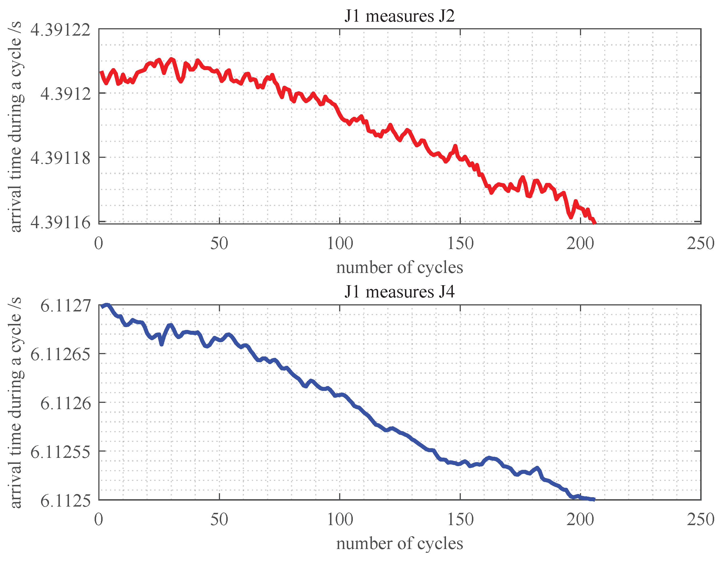
Figure 14.
Measurement timestamp of J2.
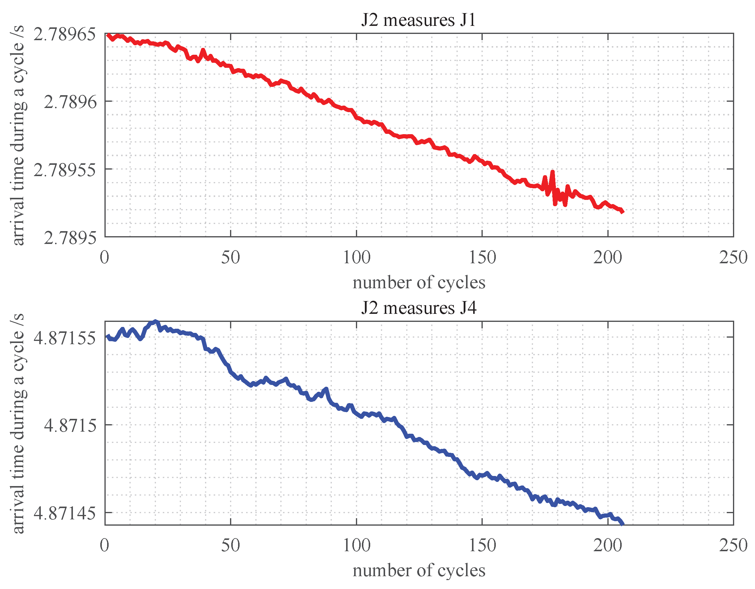
Figure 15.
Measurement timestamp of J4.
4.2. Experimental Results
Comparison between the single-cycle interaction model and the multicycle interaction model.
The experiment collected data from 206 cycles, although data from a single cycle is sufficient to solve for the beacon clock offset, as shown in Figure 16 andFigure 17. As redundant messages increase, the width of the peak gradually decreases, and the precision of synchronization progressively improves, approaching the resolution . The measurement accuracy of J2 is higher than s, while the measurement accuracy of J4 exceeds s. With increasing redundant messages, the peak width gradually narrows, and the synchronization precision progressively improves, convergent towards the resolution .
Comparison of Probability Graph Method and Conventional Time Synchronization under Single Node
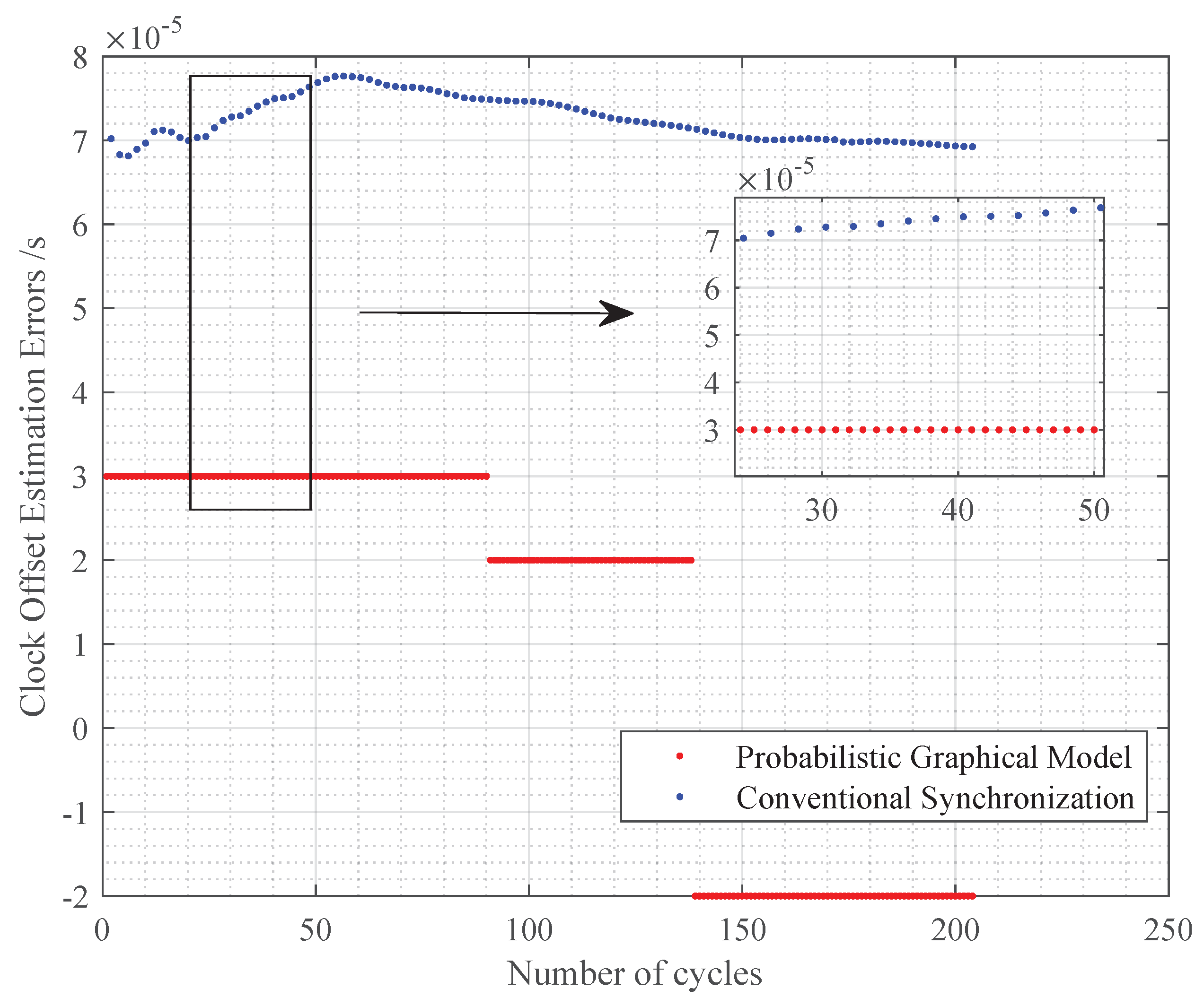
The comparison of the estimation results between the probabilistic graphical method and the Conventional Synchronization Methods (taking DE-Sync as an example) at different interaction frequencies is shown in Figure 18 and Figure 19. For the J2 beacon, the accuracy of the probabilistic graphical method is higher than , while the accuracy of the DE-Sync method approaches . For the J4 beacon, the accuracy of the probabilistic graphical method is higher than , while the accuracy of the DE-Sync method approaches. The clock offset estimation precision of both methods is of the same order of magnitude. However, the minimum synchronization cycle for a single beacon using the probabilistic graphical method is 3.4s, whereas the DE method requires 5 s and its cycle is limited by propagation delay, resulting in lower synchronization efficiency.
5. Discussion
This paper innovatively proposes an underwater network time synchronization method suitable for cluster targets, making full use of the known physical information between underwater sensor networks and greatly improving synchronization efficiency while maintaining synchronization accuracy. This method solves the problem of low efficiency in existing underwater time-synchronization algorithms when synchronizing time for multiple targets. After completion of the construction of the factor graph model for the known physical information between underwater sensor networks, the edge probability density function of the clock difference is quickly calculated to solve the clock difference parameters between units in the underwater sensor network. The experimental results show that, on the premise that its time synchronization accuracy is higher than , its synchronization period is only limited by the maximum clock difference in the cluster and can complete the timing of the entire network within a cycle. When the accuracy of arrival time measurement is not higher than and the resolution is , the estimation of time synchronization reaches the submillisecond order and the network synchronization efficiency is better than , meeting the general requirements of underwater sensor networks.
Author Contributions
Conceptualization, Y.O. and Y.Han; methodology, Y.O.; software, Y.O.; validation, Y.O., Z.W. and Y.He; formal analysis, Y.O.; investigation, Y.O.; resources, Y.Han; data curation, Y.O.; writing—original draft preparation, Y.O.; writing—review and editing, Y.O., Z.W. and Y.He; visualization, Y.O.; supervision, Y.Han; project administration, Y.Han; funding acquisition, Y.Han All authors have read and agreed to the published version of the manuscript.
Funding
Please add: This research was funded by the marine elastic PNT test system (national key research and development plan). Project No.: 2020YFB0505805.
Institutional Review Board Statement
Not applicable.
Informed Consent Statement
Not applicable.
Written informed consent has been obtained from the patient(s) to publish this paper.
Data Availability Statement
Data cannot be made publicly available due to privacy restrictions. Data are available from [Harbin Engineering University] for researchers who meet the criteria for access to confidential data.
Acknowledgments
This paper is the result of the construction and application demonstration of the marine elastic PNT test system (national key research and development plan). Project No.: 2020YFB0505805.
Conflicts of Interest
The authors declare no conflicts of interest.
Abbreviations
The following abbreviations are used in this manuscript:
| GNSS | Global Navigation Satellite System |
| NTP | Network Time Protocol |
| PTP | Precision Time Protocol |
| FTSP | Flooding Time Synchronization Protocol |
| RBS | Reference Broadcast Synchronization |
| DMTS | Delay Measurement Time Synchronization for Wireless Sensor Networks |
| TPSN | Time Synchronization Protocol for Sensor Networks |
| DE-Sync | Doppler-Enhanced Time Synchronization |
References
- Burbank,J.;Mills,D. Network Time Protocol Version 4: Protocol and Algorithms Specification. Heise Zeitschriften Verlag 2010.
- Lee,K.;Eidson,J. IEEE 1588 standard for a precision clock synchronization protocol for networked measurement and control systems. IEEE, 2002 2002. [CrossRef]
- Sivrikaya, F.; Yener, B. Time synchronization in sensor networks: a survey. IEEE Network 2004, 18(4), 45–50. [Google Scholar] [CrossRef]
- Elson, J. Fine-grained Network Time Synchronization using Reference Broadcasts. In Proceedings of the Conference on Embedded Networked Sensor Systems (SenSys’03); 2003.
- Maroti, M.; Kusy, B.; Simon, G. et al. The flooding time synchronization protocol. 2004.
- Ping, S. Delay Measurement Time Synchronization for Wireless Sensor Networks. Irb 2003.
- Xu, M.; Liu, G. Research on Cluster-Based Time Synchronization Technology in Underwater Acoustic Sensor Networks. Comput. Appl. 2013, 30, 4–10. [Google Scholar]
- Ganeriwal, S.; Kumar, R.; Srivastava, M.B. Timing sync protocol for sensor networks. In Proceedings of the International Conference on Embedded Networked Sensor Systems, Los Angeles, CA, USA, 05 November 2003; pp. 139–150.
- Wang, S.; Gao, M.; Xu, N. Research on Energy-Optimal Clustering Time Synchronization for Underwater Acoustic Sensor Networks. Comput. Sci. Technol. Dev. 2017, 27, 5–10. [Google Scholar]
- Kong, W.; Liu, G. Cluster-Based Dual-Cluster Head Time Synchronization Algorithm for Underwater Sensor Networks. Comput. Eng. 2020, 46, 8–14. [Google Scholar]
- Chang, S.; Li, J.; Gao, H. , et al. AUV-Assisted Time Synchronization Algorithm for Underwater Sensor Networks. Sens. Microsyst. 2015, 10, 137–140. [Google Scholar]
- Guo, Y.; Zhang, Z. Research on Time Synchronization for Large-Scale Underwater Sensor Networks. Electron. Inf. Sci. 2014, 36, 6–12. [Google Scholar]
- Feng, X.; Wang, Z.; Zhu, X. , et al. Research on Doppler-Assisted Time Synchronization Mechanism for Underwater Sensor Networks. J. Commun. 2017, 38, 7–16. [Google Scholar]
- Wang, H. Research on Time Synchronization Algorithm for Underwater Sensor Networks Based on Mobile Models. J. Commun. 2016, 37, 9–16. [Google Scholar]
- Huang, H.Q. Research on Passive Clock Synchronization Technology for Underwater Hidden Nodes. Ph.D. Dissertation, Xiamen University, Xiamen, China, 2018. [Google Scholar]
- Zennaro, D.; Tomasi, B.; Vangelista, L., et al. Light-Sync: A Low Overhead Synchronization Algorithm for Underwater Acoustic Networks In Proceedings of the OCEANS 2012, Yeosu, South Korea, 2012.
- Rhee, I. K.; Lee, J.; Kim, J. et al. Clock Synchronization in Wireless Sensor Networks: An Overview. Sensors 2009, 9, 56–85. [Google Scholar] [CrossRef] [PubMed]
- Sun, C.; Yang, F.; Ding, L. et al. Multi-hop Time Synchronization for Underwater Acoustic Networks. In Proceedings of the OCEANS 2012, Hamburg, Germany, 2012.
- Wen, J.; Ding, L.; Yang, F. et al. Improved Multi-hop Time Synchronization for Underwater Acoustic Networks. In Proceedings of the International Conference on Wireless Communications & Signal Processing, 2013.
- Shams, R.; Otero, P.; Aamir, M. et al. Joint Algorithm for Multi-Hop Localization and Time Synchronization in Underwater Sensor Networks Using a Single Anchor. IEEE Access 2021, 99, 1–7. [Google Scholar]
- Knapp, C. H. The Generalized Correlation Method for Estimation of Time Delay. IEEE Trans. Acoust. Speech and Signal Processing 1976, 24, 320–327. [Google Scholar] [CrossRef]
- Zhou, F.; Wang, Q.; Nie, D.H.; et al. DE-Sync: Doppler-Enhanced Time Synchronization for Mobile Underwater Sensor Networks. Sensors 2018, 18, 10–17. [Google Scholar] [CrossRef] [PubMed]
Figure 1.
Underwater Sensor Network Topology
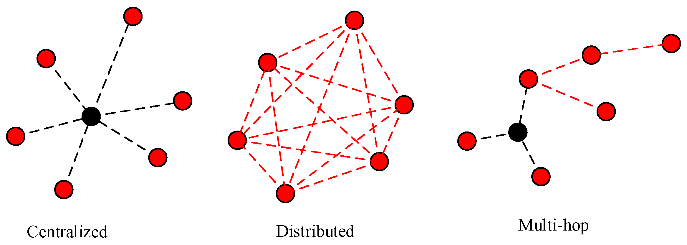
Figure 3.
Network topology structure of time synchronization Methods based on probabilistic graphical models.
Figure 3.
Network topology structure of time synchronization Methods based on probabilistic graphical models.
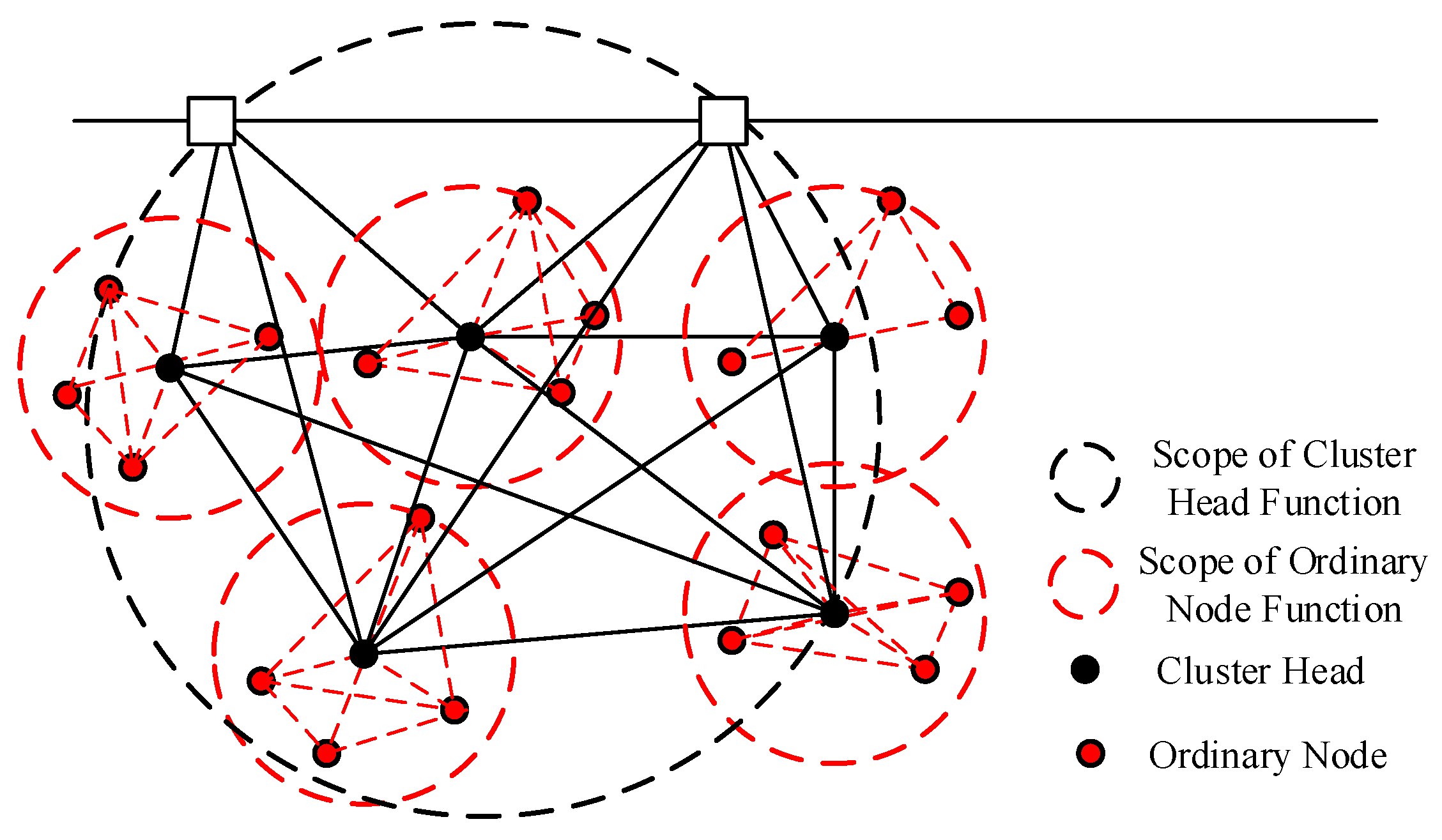
Figure 4.
Cluster-assisted probabilistic graphical model network topology structure.
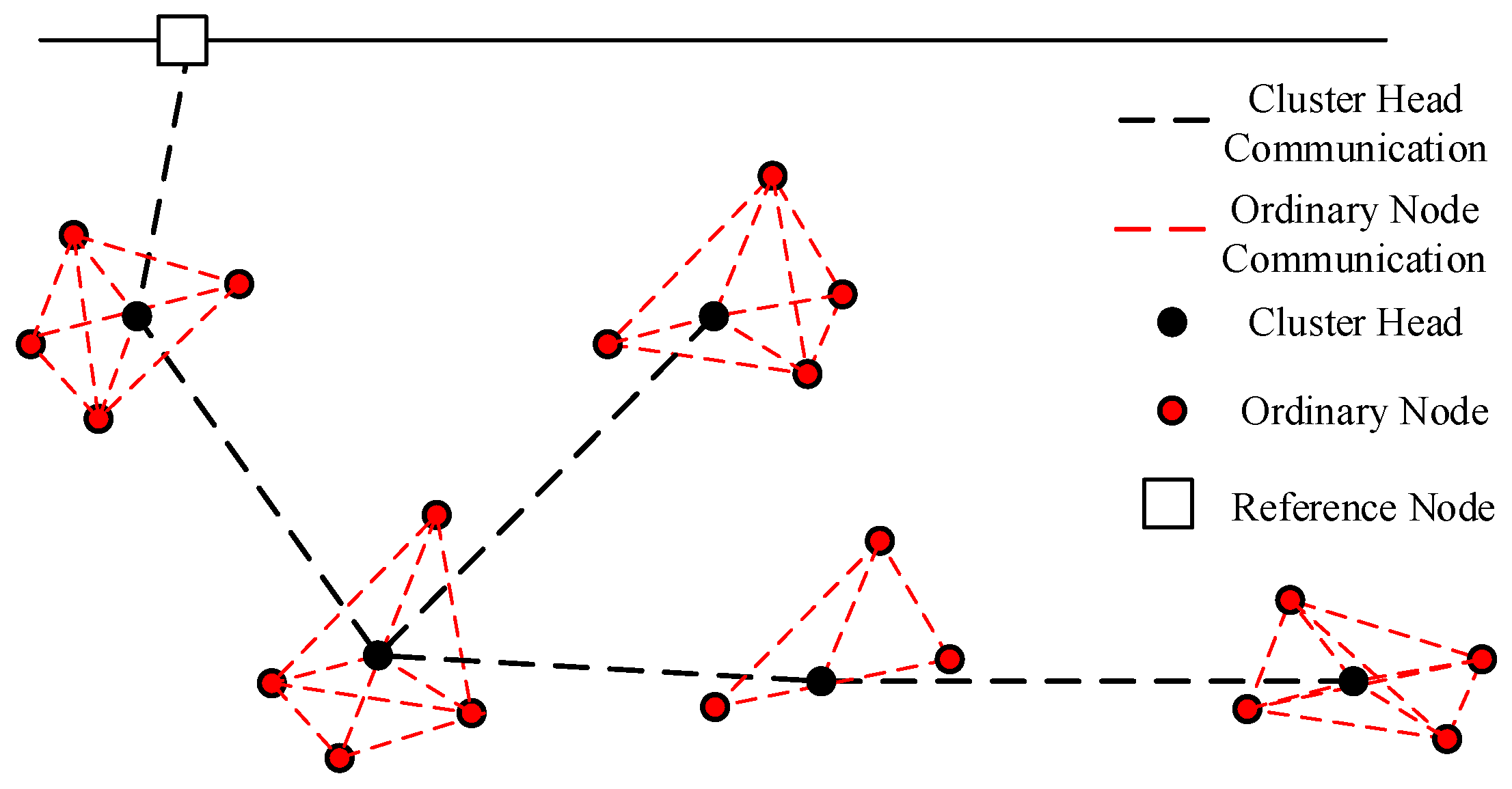
Figure 5.
Schematic diagram of intra-cluster time synchronization .
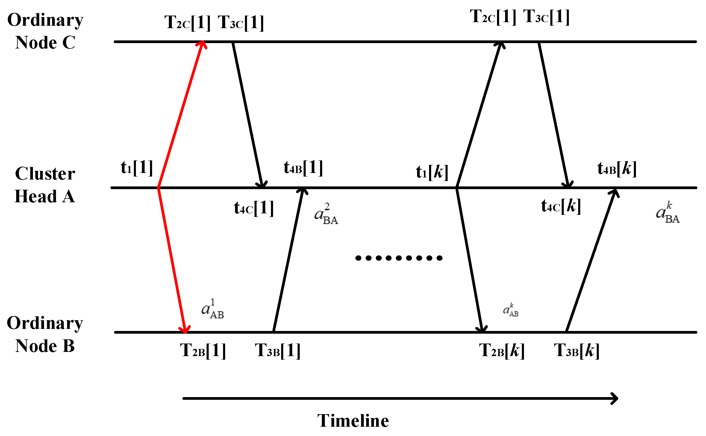
Figure 6.
Schematic diagram of intra-cluster time synchronization.
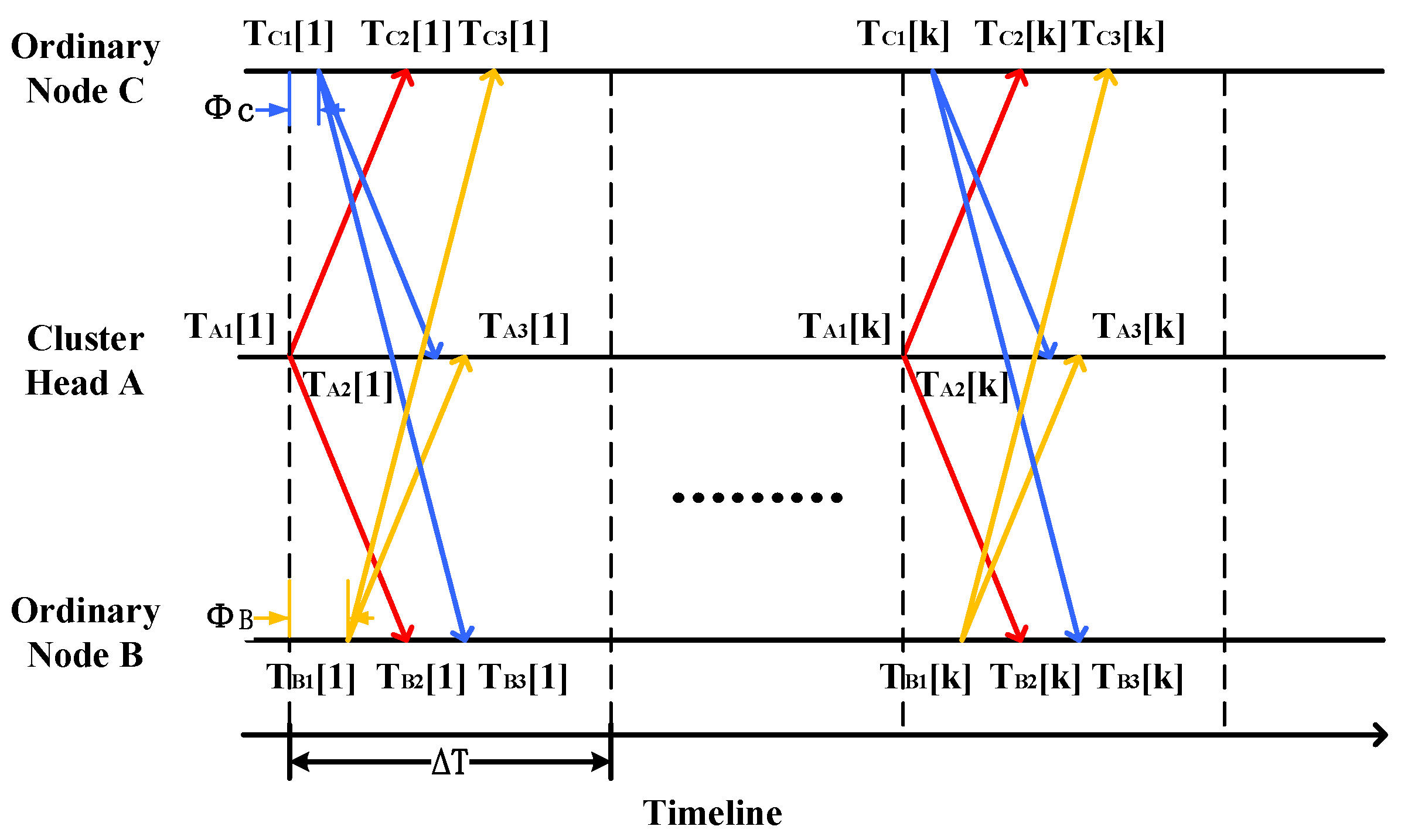
Figure 7.
Factor graph model for single-cycle underwater network time synchronization.

Figure 11.
Schematic diagram of sea trial beacon positions.
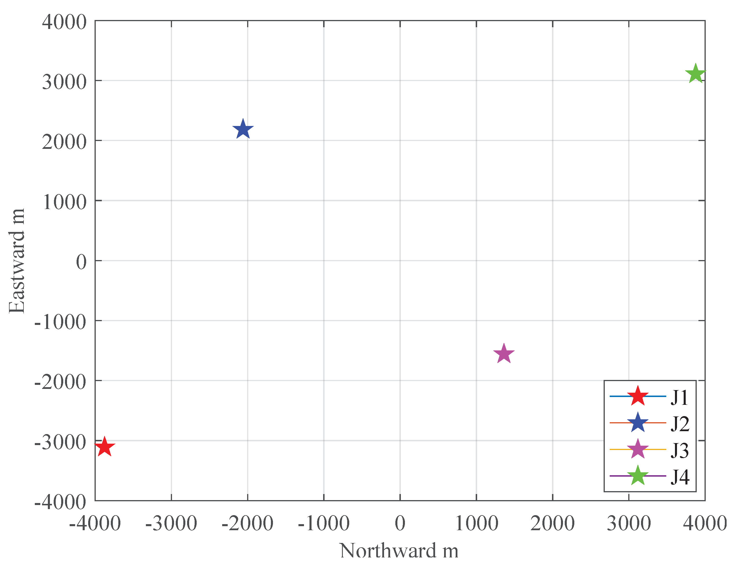
Figure 12.
Acoustic Velocity Profile.
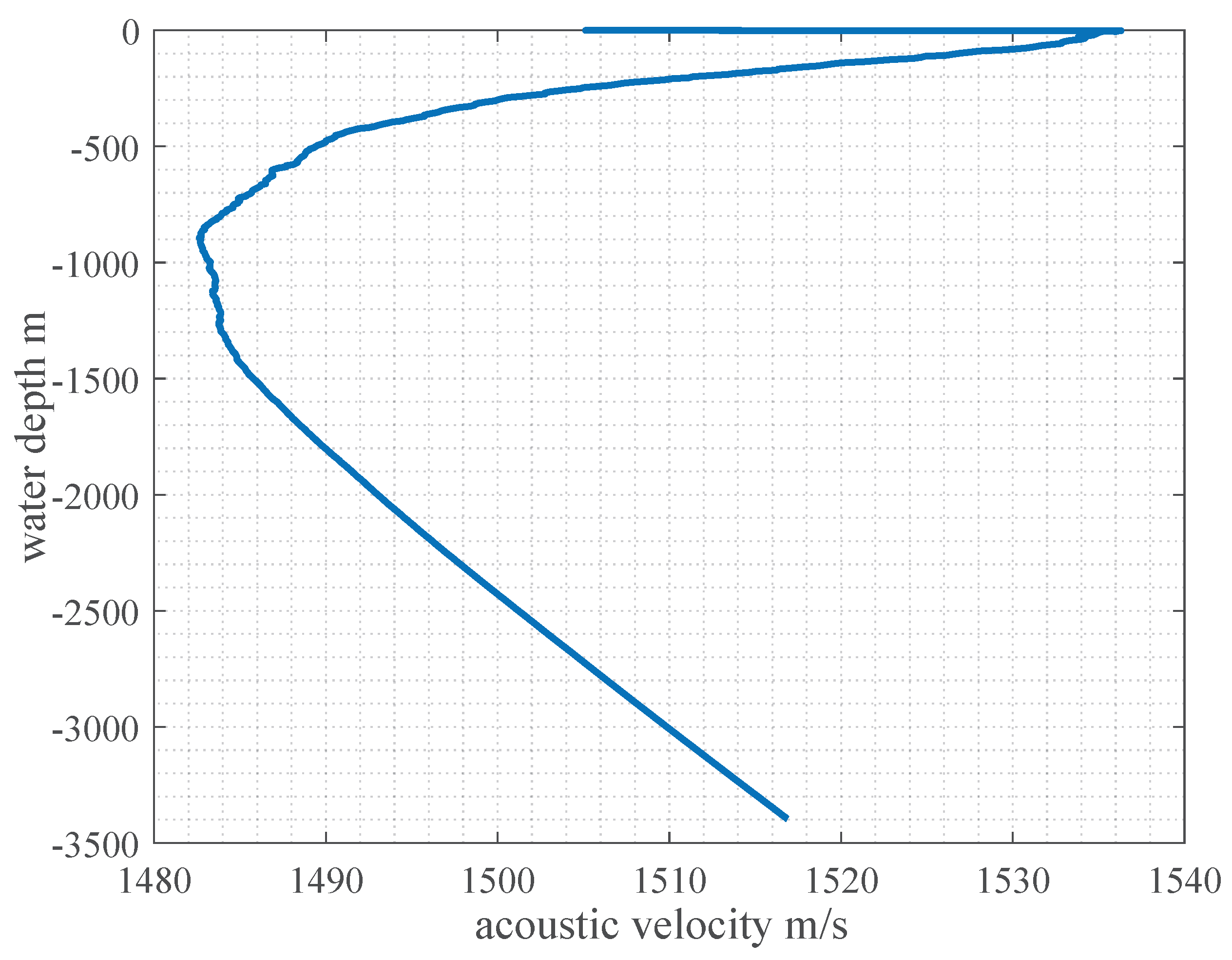
Figure 16.
Clock offset estimation of J2.

Figure 17.
Clock offset estimation of J4.
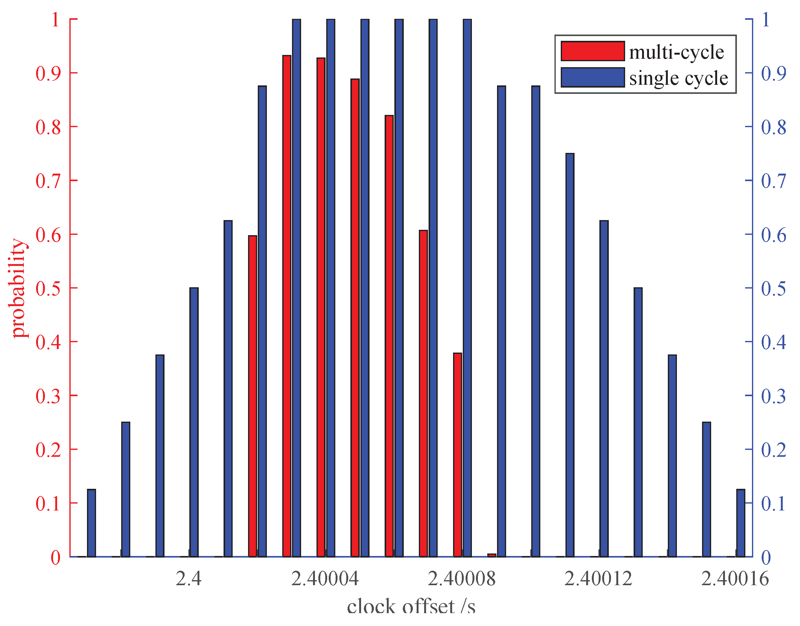
Figure 18.
Comparison of clock offset estimation errors for J2.
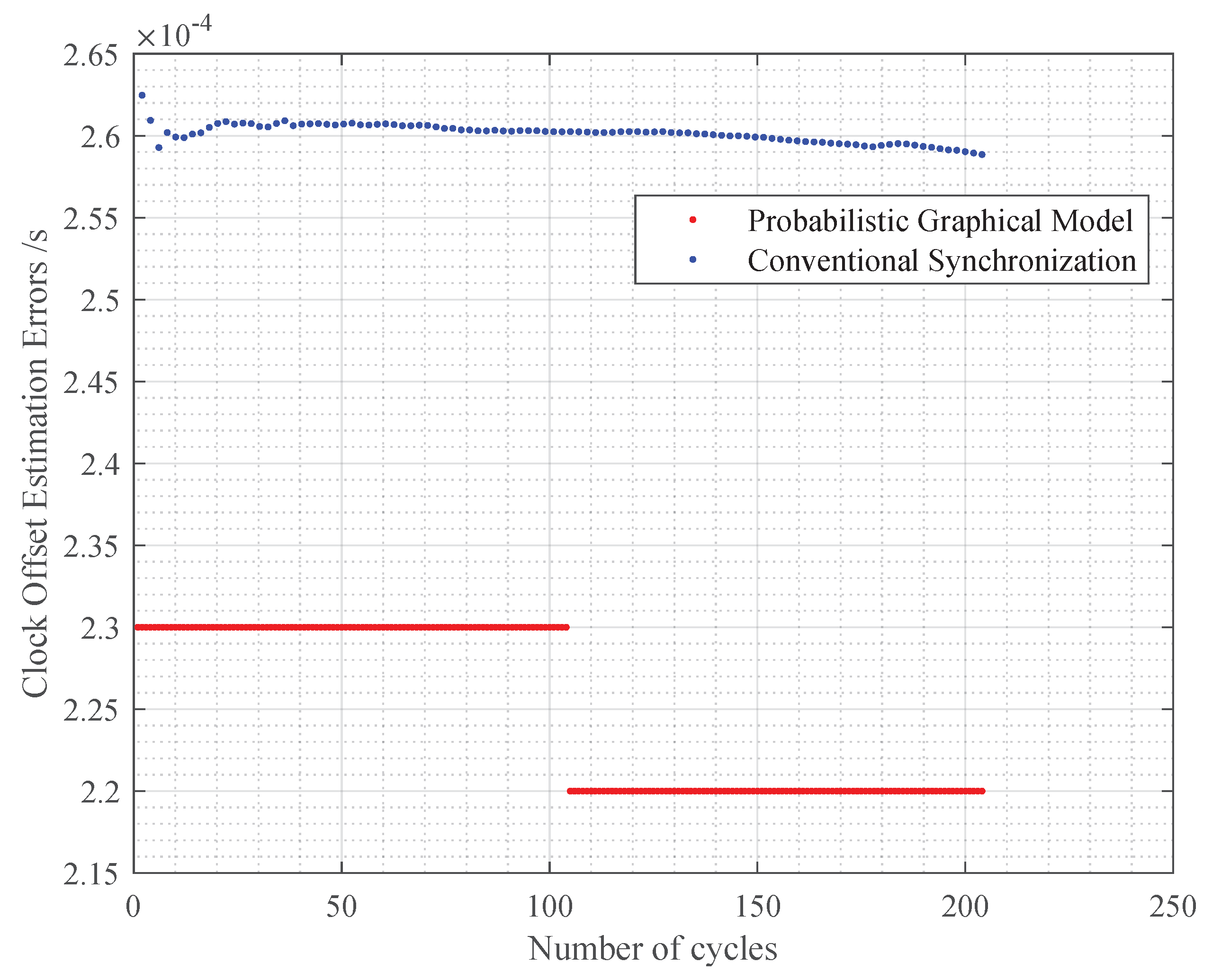
Figure 19.
Comparison of clock offset estimation errors for J4.
Disclaimer/Publisher’s Note: The statements, opinions and data contained in all publications are solely those of the individual author(s) and contributor(s) and not of MDPI and/or the editor(s). MDPI and/or the editor(s) disclaim responsibility for any injury to people or property resulting from any ideas, methods, instructions or products referred to in the content. |
© 2024 by the authors. Licensee MDPI, Basel, Switzerland. This article is an open access article distributed under the terms and conditions of the Creative Commons Attribution (CC BY) license (http://creativecommons.org/licenses/by/4.0/).
Copyright: This open access article is published under a Creative Commons CC BY 4.0 license, which permit the free download, distribution, and reuse, provided that the author and preprint are cited in any reuse.


