1. Introduction
Whale songs are frequently recorded on the hydrophones of the International Monitoring System (IMS) hydroacoustic network of the Comprehensive Nuclear-Test-Ban Treaty Organization (CTBTO) [
1]. A map showing the locations of all IMS stations, including the hydracoustic stations, is openly available [
2]. The larger whales, such as blue whales —
Balaenoptera musculus — and fin whales —
Balaenoptera physalus —, emit acoustic energy in the [15-50] Hz frequency range [
3], which can be used to assess the suitability of simple ocean-acoustic wave propagation models to estimate the location of the whales. A lot is unknown about whale vocalization (acoustic signal emitted by whales). Such questions as: the depth at which they emit the sound; if they emit the sound when only at certain depths; the depth-dependent interference of the direct signal with the surface reflection; the possible frequency — and depth — dependent radiation pattern of the acoustic emission, etc.., Attempts have been made to estimate the range from the in-water hydrophone IMS stations at which the signals are recorded. Even far ranges are considered in these attempts as it is well known that acoustic energy can travel very efficiently if it is guided in the Sound Fixing and Ranging (SOFAR) channel [
4]. Five of the six in-water hydrophone IMS stations consist of pairs of triplets of hydrophones close to oceanic islands. These island stations have one triplet deployed to the north and the other to the south of the island with the hydrophone deployment depths close to the general considered depth of the SOFAR channel of approximately 1000 m. This hydrophone depth provides excellent detections of hydro-acoustic signals originating from very far distances of 1000 s of kilometers if trapped in the SOFAR channel. The acquisition system of the hydrophones has a sampling frequency of 250 Hz which allows recordings of signals almost undisturbtly up to 100 Hz.
Previous works were concerned with whale tracking methods for basic understanding of animal behavior and mitigation of seismic airgun surveys on the animals. Methods have been developed to estimate the depth of a diving sperm whale —
Physeter macrocephalus— from the time difference between the direct arrival and the surface reflection, using two or three elements vertical or horizontal hydrophone arrays [
5]. Triangulation has been used to track the diving behavior of bowhead whales —
Balaena mysticetus — in the noisy environment of a seismic airgun survey [
5]. In both these examples, the signals emitted by the animal cover higher frequencies ([5-20] kHz and short duration < 25 ms) for sperm whales, and [0.2-2] kHz for bowhead whales). These higher frequencies are above the useful frequency range of the IMS hydrophones, and the present work studies signals emitted by likely fin whales, at frequencies below 0.1 kHz. Whale tracking has also been used in to compare the source level of fin whale signals recorded at an in-water hydrophone location in the Pacific Ocean and an Ocean Bottom Seismometer (OBS) in the Atlantic Ocean [
7]. Parabolic equation modeling is the central tool used to derive the source level of fin whales in the two regions [
8].
Other works do not specifically track whales but rather use characteristics of their calls and spatial and temporal statistics of the calls, for instance to get information on the population of blue whales in the southeast Indian Ocean and southwest Pacific Ocean [
9]. Temporal statistics have put in evidence that the dominant frequency of pygmy blue whales decreases with time over a period of 8 years [
10], and that the range of detectability of pygmy blue whales was estimated to be between 50 km and 200 km from the HA01 triplet [
11]. A range estimate of up to several tens of kilometers from the northern triplet of HA08 in the Chagos archipelago in the Indian Ocean, was obtained using a method based on two parameters: back-azimuth estimates using the signals on the three hydrophones; and amplitude decay estimates [
12]. At these distances, based on modeling up to 250 km, the amplitude of the whale signal decays roughly like the square root of the distance to the hydrophone, as expected from a cylindrical geometrical spreading. The calls were detected in records from January 2003 with a Short-Term Average/Long-Term Average (STA/LTA) method using a ratio threshold of 2.5.
At closer range, it is possible to make the assumption that the whale is close to the surface (whale depth is assumed to be zero), and then use the differences in the times of arrivals between the three hydrophones to estimate a location. This method was used to trace the path of a likely fin whale crossing the waters above hydrophone station HA01, Cape Leeuwin, Australia [
13]. In that work, the authors tracked the movement of the whale through the three hydrophones using the direct arrival from the whale signal. They also observed multiple scattered energy — one directly from the ocean bottom, another from the sea surface after reflection from the ocean bottom — as the whale position was close to being in the area directly above the hydrophones. Similar multiple scattered arrivals from the ocean bottom and sea surface had previously been observed in bottom-moored hydrophones in the Southern Ocean [
14]. In addition to water multiple reflections, crustal reflections were observed from fin whale calls recorded on ocean bottom seismometers in the straights of Juan de Fuca, between the USA and Canada [
15].
Tagged animal studies on fin and blue whales [
16] have been conducted and show some variability in the swimming depth of a fin whale between very shallow depth (10 m) and up to nearly 300 m. A deeper dive may occur amidst shallower ones. At shallow depths of vocalization of a fin whale, somewhere between the sea surface and 300 m depth, it may be difficult to differentiate in time between the direct path from the animal to the hydrophone, and the reflection from the sea surface. In [
13], a double peak in the autocorrelation and envelope of the first arrival may hint at this sea surface reflection. An elaborate approach [
17] based on modeling Lloyd’s mirror effect [
18] estimated the depth of vocalizing fin whales using the hydrophone and vertical component seismometer channels of Ocean Bottom Seismometers (OBS) and estimated a depth of 72 m in one of the examples. A shallow depth of 15 m was also estimated, for an individual fin whale localization, based on the modeling of travel times of multiple bottom and surface reflections, at the three hydrophones of the southern triplet of IMS hydroacoustic station HA11 [
19]. In the present work, data processing and location methods are applied to a data set recorded at the same hydrophone triplet, on 19 and 20 February 2024. A fin whale passed close to the triplet, similarly to the 26 July 2017 at HA01 [
13], and the multiple passages at HA11, between 2010 and 2022 [
19]. In addition to the use of travel time differences for location purposes, we compare observed amplitudes to estimated amplitudes from using a simple model with spherical spreading when whales are assessed to be at short range, within a 1.5 km of the center of the hydrophone triplet.
The next section introduces the 2024 data set, and the methods used to process the data and to find the vocalization locus of a passing fin whale assuming it is vocalizing at shallow depths. The parameters used in the localization are the time delays — or Time Differences of Arrival (TDOA) —between arrivals for the same call at three hydrophones in a triplet. An estimate of the depth of vocalization of the whale when located near two of the hydrophones is made later based on the amplitude ratios of these arrivals and the assumption that the amplitude decays as the inverse of the distance to the hydrophones. Based on a fit of the amplitude ratios for the same signal at the three hydrophones to the ratios of the distances to these hydrophones, an assessment of the values published for the hydrophone location and depths is also made. Applying a correction to these locations would better explain the amplitude data.
2. Data Acquisition and Processing Methods
2.1. Data Acquisition
The data set analyzed in this work was acquired at IMS hydroacoustic stations HA11.
Table 1 shows basic site location parameters for the hydrophones H11S1, H11S2, and H11S3 of the southern triplet of the station HA11S. For the reminder of this work, the identifiers S1, S2, S3, as shown in
Table 1 will be used for respectively H11S1, H11S2, and H11S3. A local coordinate system has the S1 hydrophone location as its origin and
Table 1 also shows the coordinates of the hydrophones in this local system.
Figure 1d is a simple local map showing the geometry of the triplet.
The data is openly available from the IRIS data center [
20] with network code IM.
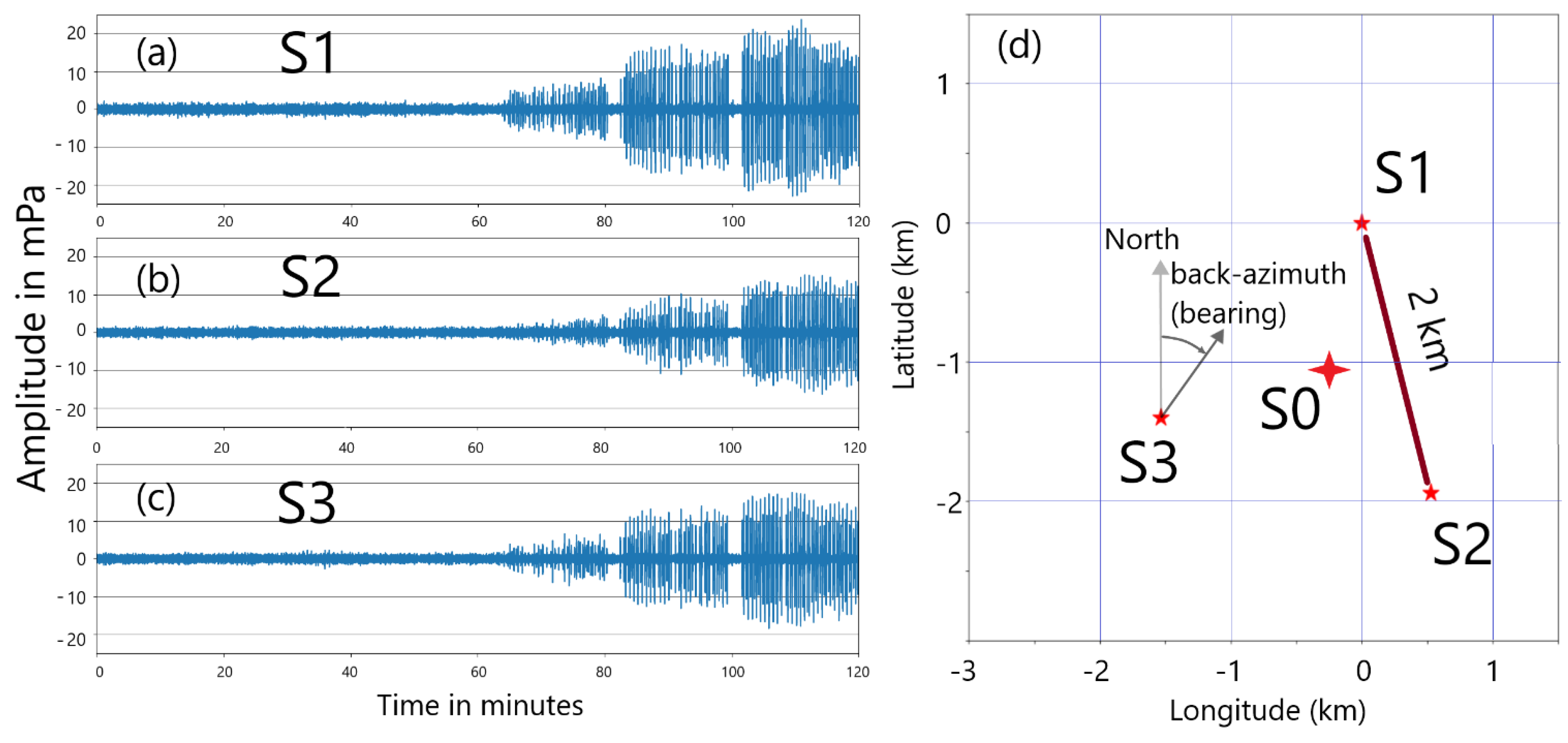
Figure 1a, 1b, and 1c show two hours of the three hydrophone traces at respectively S1, S2, and S3 at the beginning of the sequence of interest, starting at 21:00 UTC on 19 February 2024. The data of interest is clearly visible on the raw waveform starting at around 22:05 UTC, sixty-five minutes after the beginning of the trace. Several observations can be made regarding the features of the signal on the three waveforms:
The amplitude of the signal is increasing on all three waveforms starting from about one hour after time zero. This can easily be explained if the source is progressively getting closer to all three sensors until the end of the two-hour sequence.
The amplitudes at S1 and S3 are slightly higher than at S2.
There appears to be interruptions of two to three minutes in the sequences of calls at every fifteen to twenty minutes. Since it is well known that cetaceans surface at regular intervals to breathe, it seems natural to infer that these short interruptions correspond to the surfacing of a single individual, or several individuals surfacing in a synchronized fashion, and that the vocalizations happen while the animal dives between the surfacing.
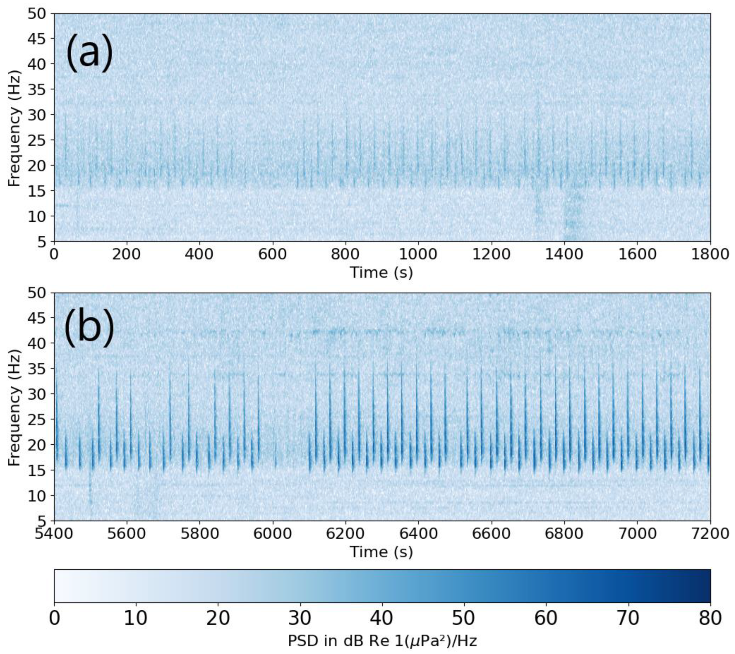
On the spectrogram for the same time interval, the beginning of the trace also shows the large amplitude individual transient arrivals in the [15-50] Hz band. This is illustrated by
Figure 2 showing the first and last 30 minutes of the two-hour interval. Observations beyond the previous ones can be made from the spectrograms:
Two types of calls are clearly visible on the spectrogram. One type has a broader bandwidth [17-40] Hz and higher centre frequency than the other one [15-25] Hz. These two types have previously been nomenclatured as type A for the lower frequency type and type B for the higher frequency [
19]. The two types are separated by about 25 s and generally alternate, but not always. An exception can be seen on
Figure 2 in an interval of about 100 s after 5600 s with three consecutive type B in that interval, and again twice at about 5800 s. This has an implication on the measurement of amplitudes, which shows a bimodal distribution as will be shown later in this work.
If the hypothesis that the interruptions in the calls are at the time of surfacing, the first call when the animal dives is the narrower lower frequency pulse (type A), and the last call is the broader, higher frequency call (type B)
2.2. Waveform Signal Processing
To estimate the location of the whale calls when the signal is strong, we start by picking individual signals out of the background noise using the STA/LTA ratio method, explained in [
22]. This method is often applied on seismic data (e.g. [
23]) for the purpose of automatic picking of seismic phases. In the present work, the STA time interval is 0.1 s and the LTA time interval 1 s. This method is also part of the hydroacoustic processing chain at the International Data Centre (IDC) of the CTBTO, as explained in detail in [
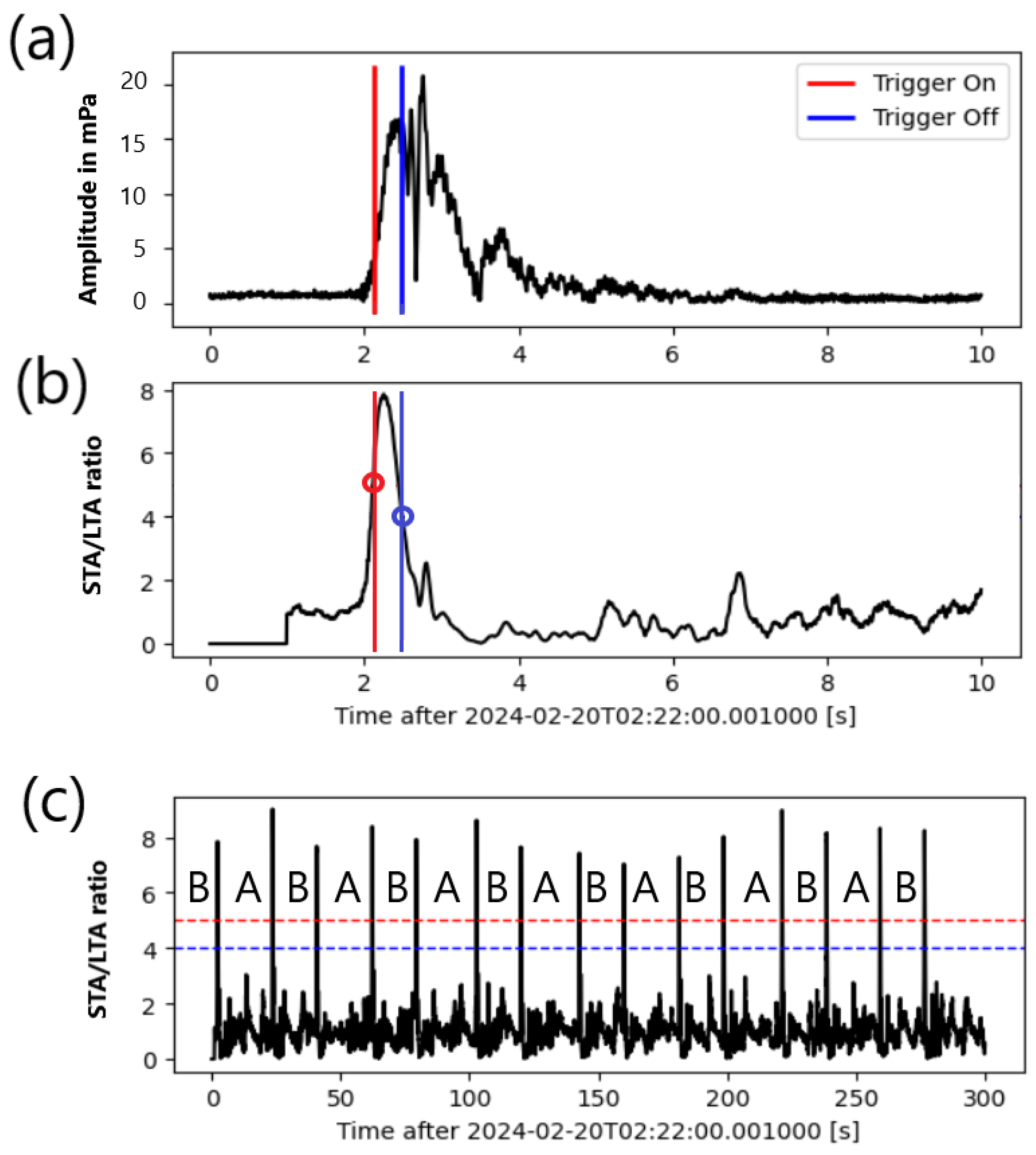
24]. In the present work, the STA/LTA method is used on the envelope of the waveform after bandpass filtering between [10-50] Hz, rather than directly on the waveforms themselves, avoiding the possible confusion between positive and negative maxima. The bandpass filter used is a fourth order Butterworth filter. This is illustrated by
Figure 3 where values of 5 for the trigger-on and 4 for trigger-off are used on a five-minute segment of data at hydrophone S1 starting at 2:20:00 UTC on the 20 February 2024. Fifteen detections are made in the time segment.
Figure 3a shows a close-up of the envelope of the first call in the sequence, which is identifed as a type B call.
Figure 3b shows the STA/LTA function for that call. For the same time interval, the same number of detections is made on the other two hydrophones, S2 and S3.
Figure 3c shows the fifteen calls, with the type identification placed before each call.
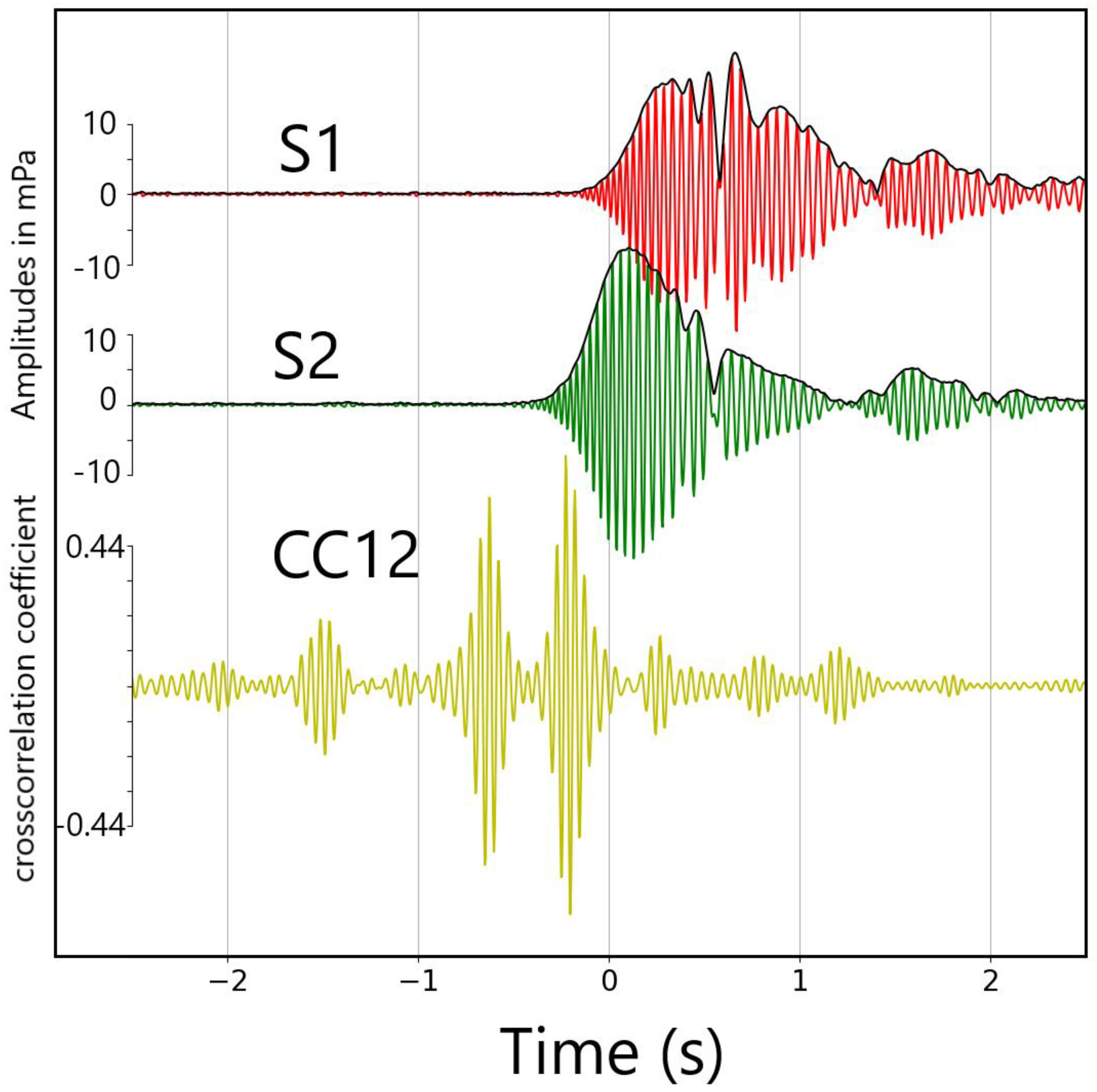
Figure 4‘s panels (a) to (c) show signals for the same call as in
Figure 3a at the three hydrophones on 10-second segments starting 2.5 seconds before the on-trigger times at hydrophone S1. TDOAs between the direct arrivals at the three hydrophones are clearly visible and emphasized by the thin blue lines on each of the three panels. They are marked as d12, d23, and d32 respectively for the delays between S2 and S1, S3 and S2, and S1 and S3.
Several methods were tested to compute TDOAs between the three hydrophones to assess a location for the source of the signals in the case when the signal is strong enough to trigger the detector with the parameters specified above:
1 – The first method is to compute TDOAs from the cross-correlations between S1 and the other two traces for each detection made at S1. The cross-correlations are computed on ten-second segments and the detection is confirmed on the three traces when the maximum of the cross-correlation is larger than 0.5.
2 – The second method is to use detections made on the other hydrophones if they fall within a three-second interval from the S1 detection. The TDOAs are then simply the time differences between the detection times.
Figure 5 illustrates the difference in TDOA computation between the two methods on the two-hour interval shown on
Figure 1. The detector found respectively 142, 124, and 131 detections on S1, S2, and S3 in that interval. Note that the first detection is made after 60 minutes, five additional detections are made between 75 and 80 minutes, and between 80 minutes and 120 minutes, the detection density is higher than two per minute.
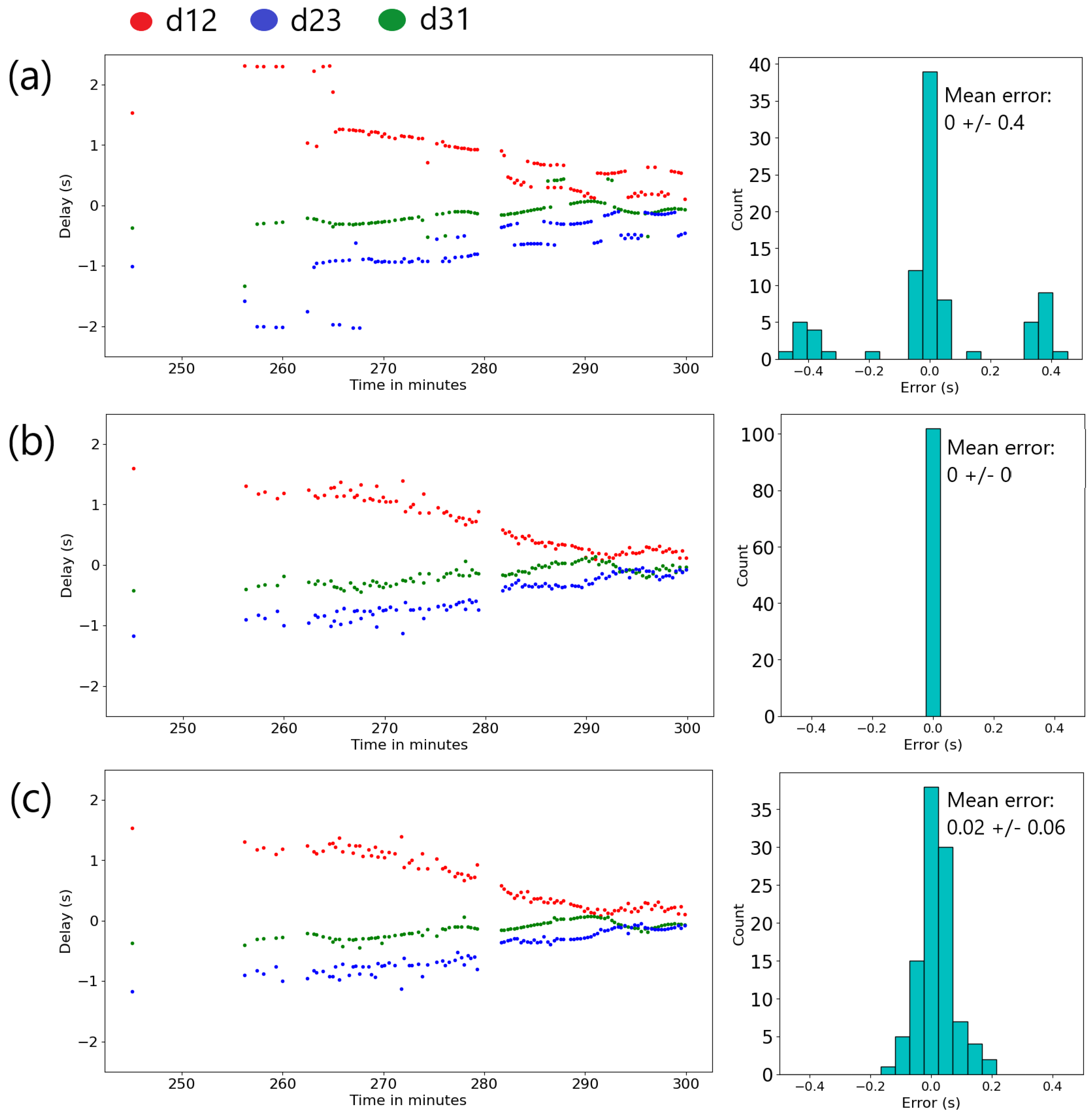
There are striking differences between the results of the two methods used to compute the delays. The cross-correlation based method 1 (
Figure 5a) shows higher consistency between the estimated values of the TDOA for consecutive calls, however there are sudden jumps in these values from one call to the next. These can be attributed to the reflected arrivals following the first arrival, which can be as large as the first arrival (see for instance S3 trace on
Figure 4). The picks-only method 2 (
Figure 5b) does not show these sudden jumps in the values of the TDOAs likely because the method ensures that the TDOAs will be computed on the first arrival and not later reflected arrivals. The consistency between two consecutive calls however is not as good as for method 1, partly because there is no guarantee that picks based on a value of STA/LTA optimize the alignment of waveforms. A natural improvement consists of using method 2 to get initial values and then refine the value of the TDOA via cross-correlation (
Figure 5c). In the remainder of this study, it will be referred to as “improved method 2”. The histograms on the right of each panel show the distribution of closure errors for each panel. The errors are always zero by construction for method 2 and can be large for method 1. This may happen for instance when the maximum of the cross-correlation corresponds to a correlation between a direct arrival and a reflected arrival. Improved method 2 shows that introducing a small shift based on the cross-correlation TDOA values increases the errors. The errors remain within a value of 0.2 seconds, however.
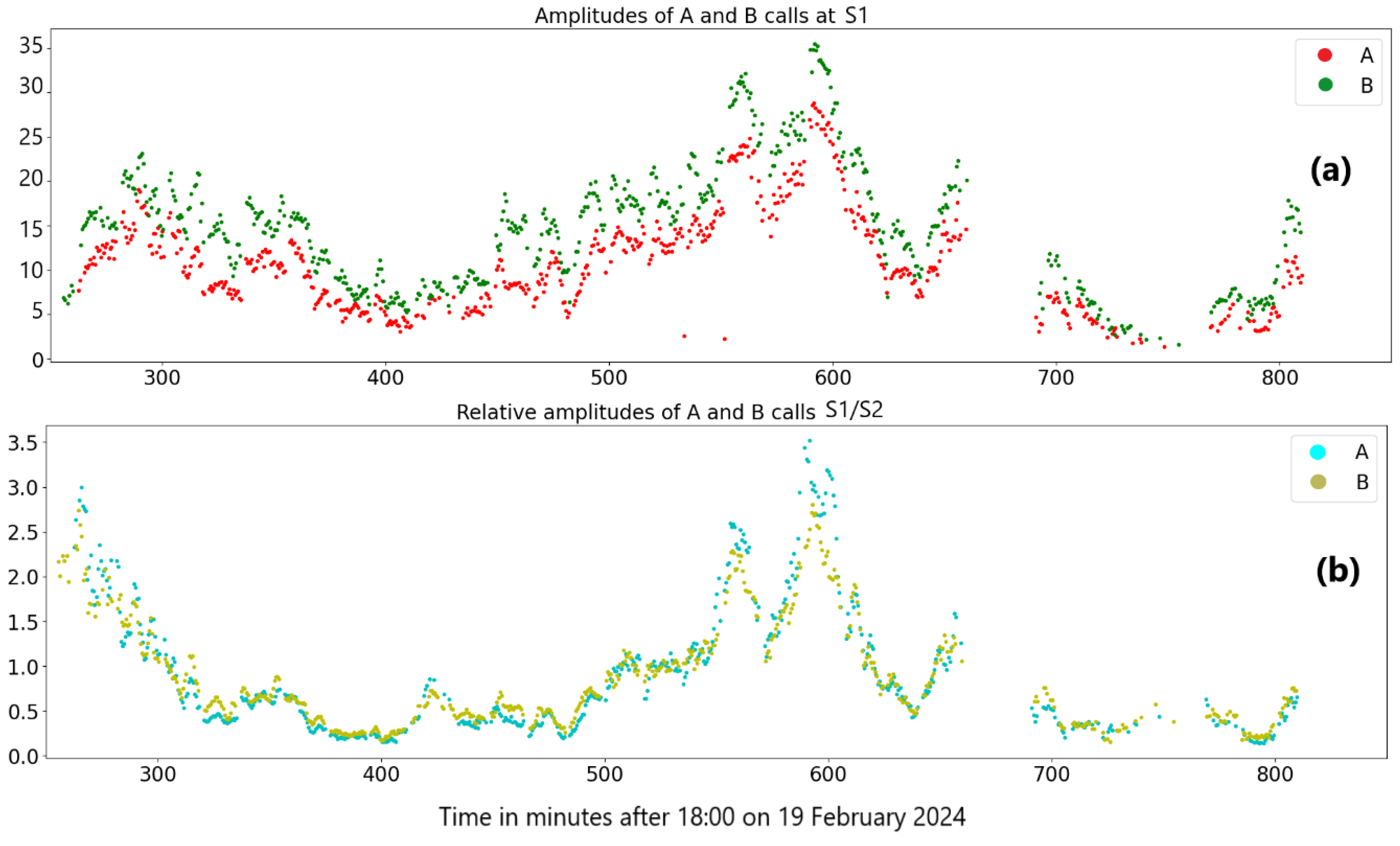
The amplitudes are computed as the maximum of the envelope in a 6s interval starting 2.5 s before the detection trigger time on S1.
Figure 6a illustrates the difference in amplitude between the A calls and the B calls. B calls have consistently higher amplitudes. When ratios are considered however, such as the ratio of the amplitude at S1 to the amplitude at S2, types A and B calls show a high degree of consistency. This will allow a comparison of this ratio to the ratio of distances once we have a location for each call.
The method described in the previous section is applicable when the calls have sufficient Signal to Noise Ratio (SNR) to be detectable via the STA/LTA (a value of 4 for the detection threshold was used in the example presented in
Figure 1,
Figure 2 and
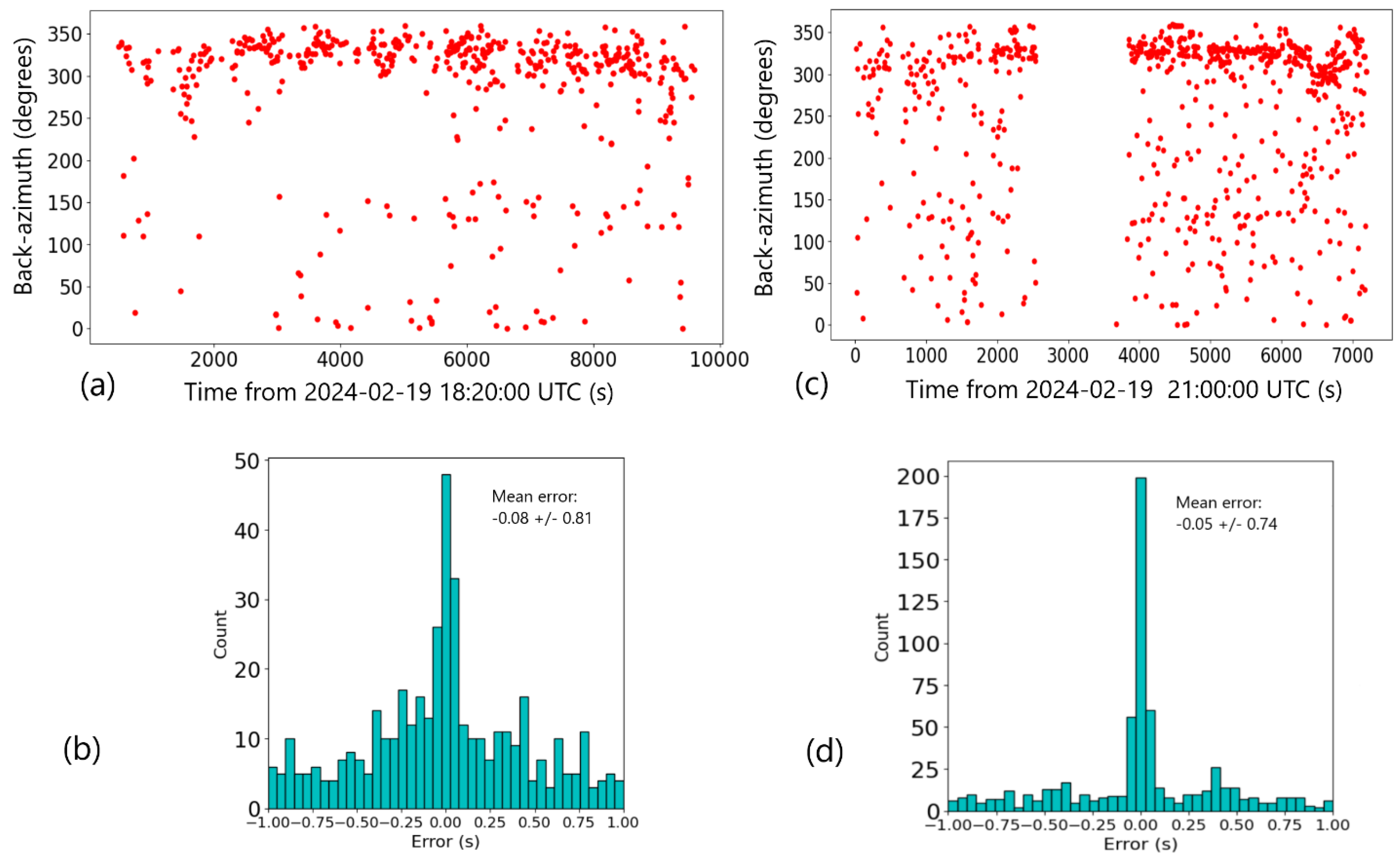
Figure 3). In the absence of sufficient energy at the receiver, it is still possible to obtain the direction of incoming signals using a cross-correlation method on segments of data, with no pre-determined picks, unlike the three methods previously mentioned. Preceding the two-hour segment studied so far, the amplitude of the signals is very low, but still visible on the spectrograms from about 18:20 UTC on 19 February 2024. The result of applying cross-correlations on segments is shown on
Figure 7 for the 2 hours and forty-minute period starting at 18:20 UTC and ending at 21:00 UTC and for the 21:00 to 23:00 UTC period previously processed based on STA/LTA picks. The computation of the TDOAs is much noisier than it is when the signal is sufficiently strong to warrant a power detector method, but the back-azimuth can still be estimated from that data and is shown on panel 7a. Clear trends are seen developing in the second hour of the segment, with a dominant back-azimuth between 300 and 350 degrees from north, and a hint of another back-azimuth 180 degrees from it, between 120 and 170 degrees. This latter back-azimuth may be due to back-scattering from the seamount known to underlie the southern triplet of H11A as described in [
21].
Figure 7a and
Figure 7c clearly show the continuity of the back azimuth between the earlier, low SNR signals (undetected with an STA/LTA threshold of 4) and the stronger signals when they reach the vicinity of the triplet of hydrophones. Panels 7b and 7d show the error estimates histograms similarly to
Figure 5. It may be possible to use amplitudes to estimate the range, as it would be expected to decay like the square-root of the distance, but this has not been attempted on this data.
2.3. Location Method by Grid Search
Since with large amplitudes (above 5000 μPa in the [10-50] Hz band), it is likely that the whale is close to the triplet of hydrophones, we assume straight line propagation and that the whale is close to the surface (whale depth is assumed to be zero). The localization of each call is then accomplished by a simple grid search to minimize the time TDOA differences between measured and modeled TDOAs at each hydrophone, assuming straight ray propagation and a water velocity of 1480 m/s. The latitude and longitude grid spacing is 25 m and the depth difference between the source and receivers is set constant during the search. Specifically, the grid search is initially done over a 12.5 by 12.5 kilometers area to locate the first call. For subsequent calls, the search is limited to an area 2.5 by 2.5 kilometers, since the animal cannot travel far from one call to the next.
3. Results
3.1. Location by Grid Search for the Minimum of Root Mean Square (RMS) of Delay Residuals
While the depth at which the whale vocalizes is an unknown, one can assume that it is shallower than the depth of the hydrophones. In a first attempt at tracking the motion of the vocalizing whale, it is assumed to be at the surface of the ocean. Improved method 2, explained in section 2.2, was used to extract the parameters of interest (absolute times of picks, TDOAs between hydrophones, amplitudes of the signal). The amplitudes are computed on the signal’s envelopes such as the one shown on
Figure 3(d). The depth will trade-off with the projection on the horizontal plane (epicentre in seismology). A way around this is when sensors are directly above the fault in seismology, or directly below the whale for the hydrophones, provided an estimate of the location and origin time are available.
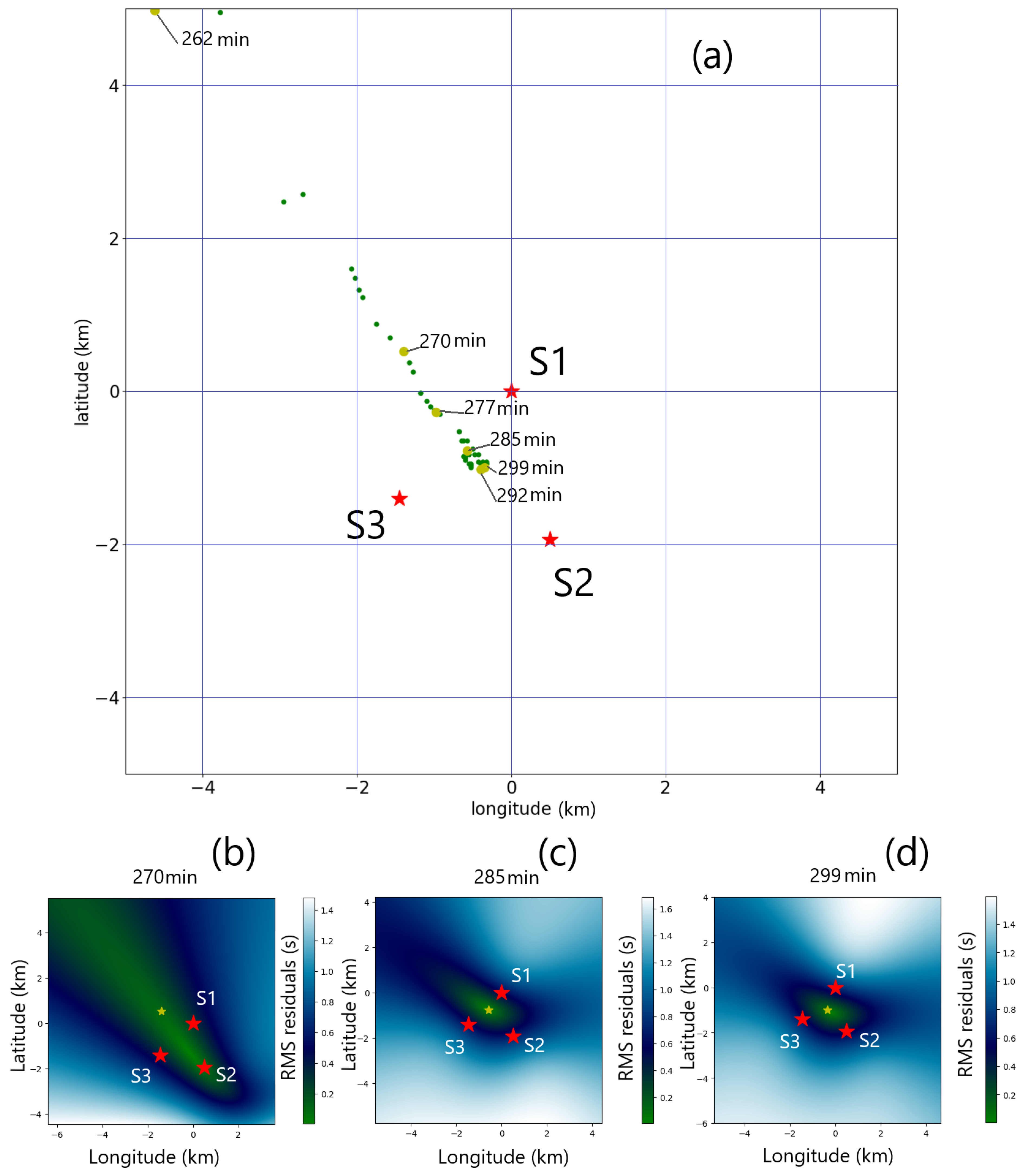
Figure 8a shows a map with the results of the localization of all 49 A calls for the two-hour data set starting at 21:00 UTC on 19 February 2024 (shown on
Figure 1). Note the progression of the whale from the northwest to the center of the triplet during this interval.
Figure 8b,
Figure 8c, and
Figure 8d are maps of the residuals for three of the points indicated by yellow dots on the map. The minimum of the residual is indicated by a yellow star and the value of the residual is shown on a 10 km by 10 km square. It is apparent that the two points (minutes 285 and 299) which fall inside the perimeter defined by the triplet have a better spatial resolution than the point (minute 270) which lays outside of the perimeter. The residual surface for that latter case has a shape elongated along the direction from the center of the triplet to its minimum. The back-azimuth from the center of the triplet is well constrained, but not the distance to the minimum.
3.2. Using the Amplitude Ratios to Assess a Simple Propagation Model
All calls between 21:00 UTC on 19 February and 14:00 UTC on 20 February with a location close to the center of the hydrophone triplets were gathered into a single data set. A value of 4 for the STA/LTA trigger-on value was used in this case, and a value of 2 for the trigger-off. A total of 597 A calls and 600 B calls were initially detected.
The assumption that the decay in amplitude is as 1/R, where R is the distance between the source and the receiver, breaks down when the propagation becomes mostly horizontal for a source far away from the triplet. As demonstrated on
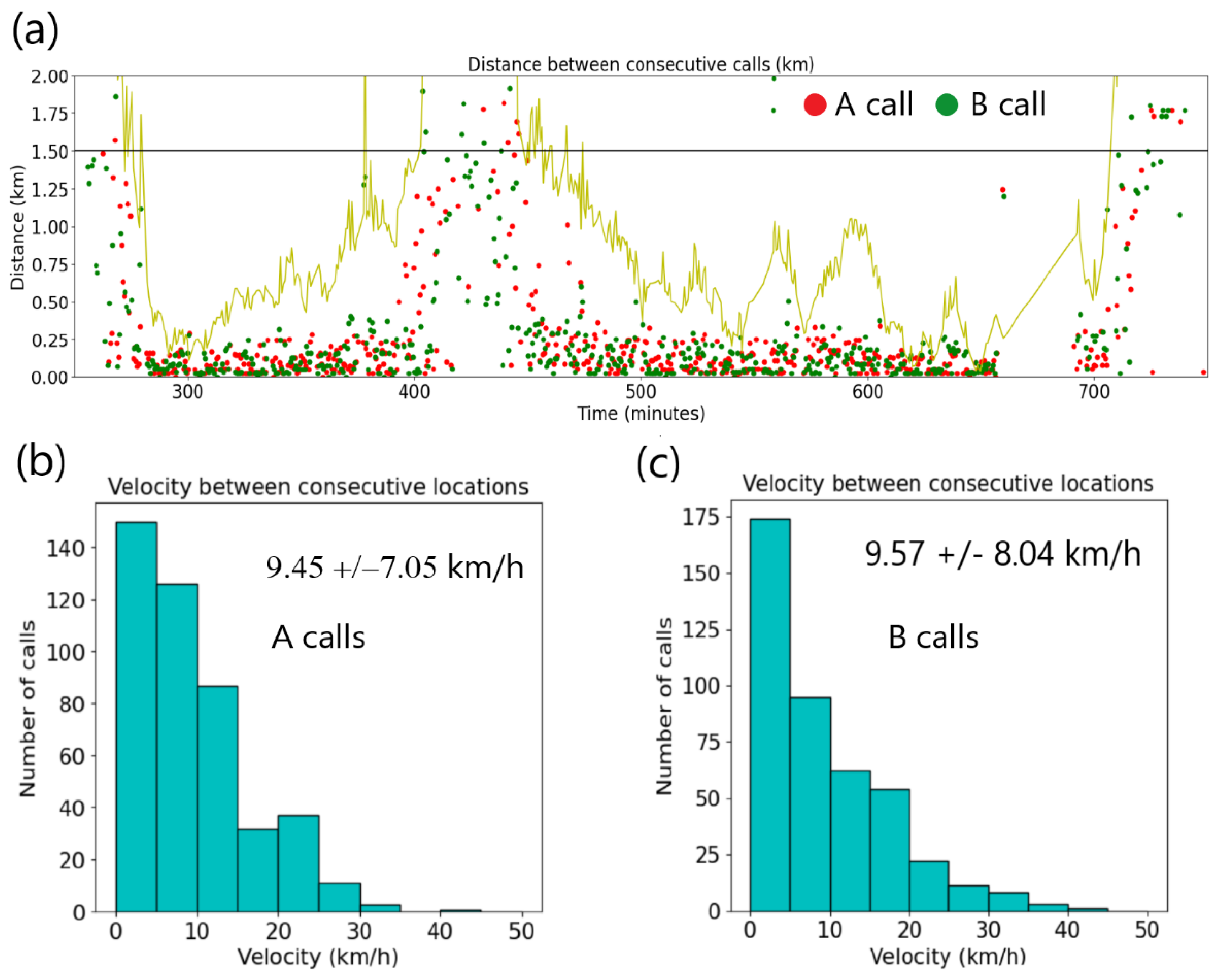
Figure 8, the uncertainty on the location of a call is greater when the whale is outside of the perimeter of the triplets. This is also reflected in the average distance between consecutive calls as shown on
Figure 9. The yellow line is the distance of the location of calls to the center of the triplet. When that distance falls below 1.5 km, shown by the solid black line, the distance between consecutive calls is concentrated around or below 0.25 km, indicating that a more accurate location is obtained inside of the circle of 1.5 km. The distances between consecutive calls have large average values and standard deviation when outside of the 1.5 km radius circle, as can be seen on
Figure 9a between approximately 400 and 450 minutes.
Figure 9 also shows the histograms of estimated swim velocity of the whale when inside the 1.5 km circle, eliminating non-physical outlier values of velocity larger than 50 km/h. This results in a reduced number of 447 A calls and 430 B calls on which velocity statistics are computed. An average value of 9.45 ± 7.05 km/h between two consecutive A calls and 9.57 ± 8.04 km/h between consecutive B calls is compatible with what is known about the swim velocity of fin whale, which have a maximum swim speed of 37 km/h, or about 20 knots [
3].
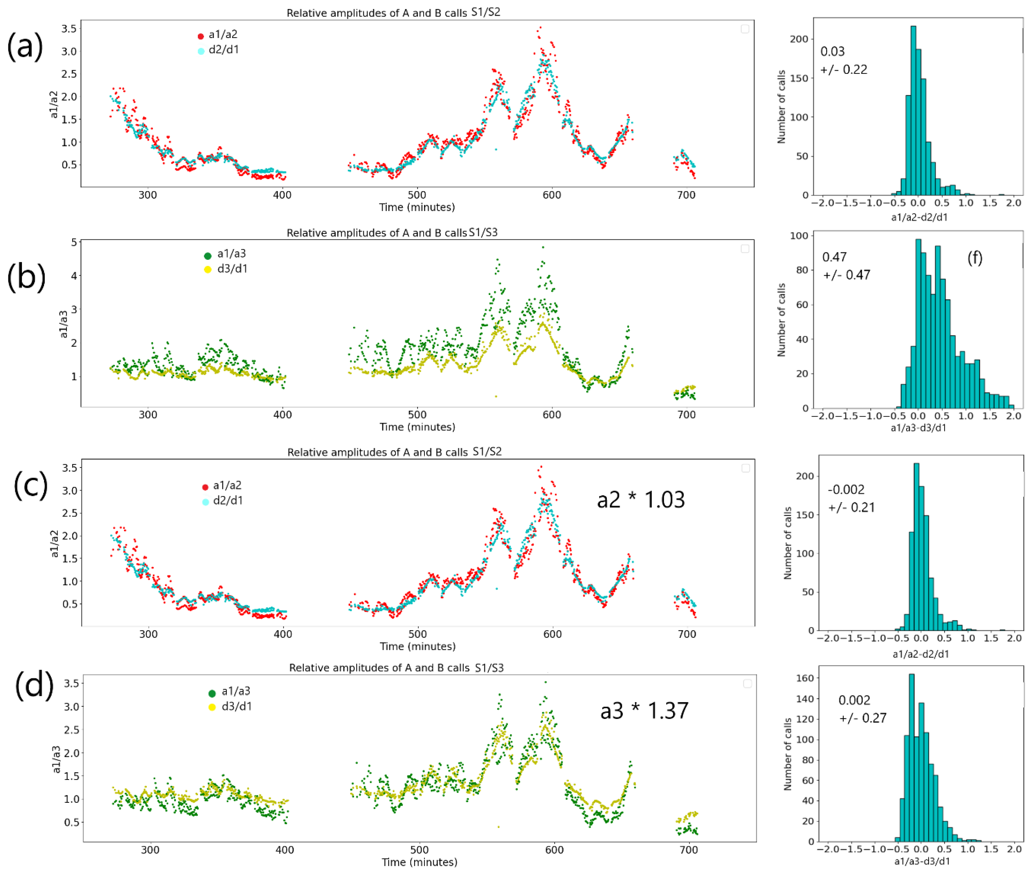
The relative amplitudes were discussed in section 2.2, and it was concluded that the A and B calls, while exhibiting different absolute amplitudes in the frequency band considered, the relative amplitudes between hydrophones show consistency between the two types of calls.
Figure 10 shows the variations and histograms of the relative amplitudes a1/a2 and a1/a3 where a1, a2, a3 are respectively the amplitudes measured at S1, S2, and S3. The measured (a1/a2) and theoretical (d2/d1) values follow each other quite closely, while a1/a3 and d3/d1 depart from each other, as emphasized by the histogram of the differences. When using only the calls within the 1.5 km limit from the center of the triplet and eliminating outliers (residuals of |a1/a2-d2/d1| more than 1 and |a1/a3-d3/d1| more than 2), the biases are computed from the average ratios of (d2/d1) to (a1/a2). The biases are respectively 1.03 for a1/a2, and 1.37 for a1/a3. If the larger bias observed at S3 originates from the need to adjust the calibration of that hydrophone, it should be possible to observe the same kind of average differences for hydroacoustic arrivals propagating horizontally on large distances before reaching the triplet, of which there is a very large database at the IDC. This is however beyond the scope of this study.
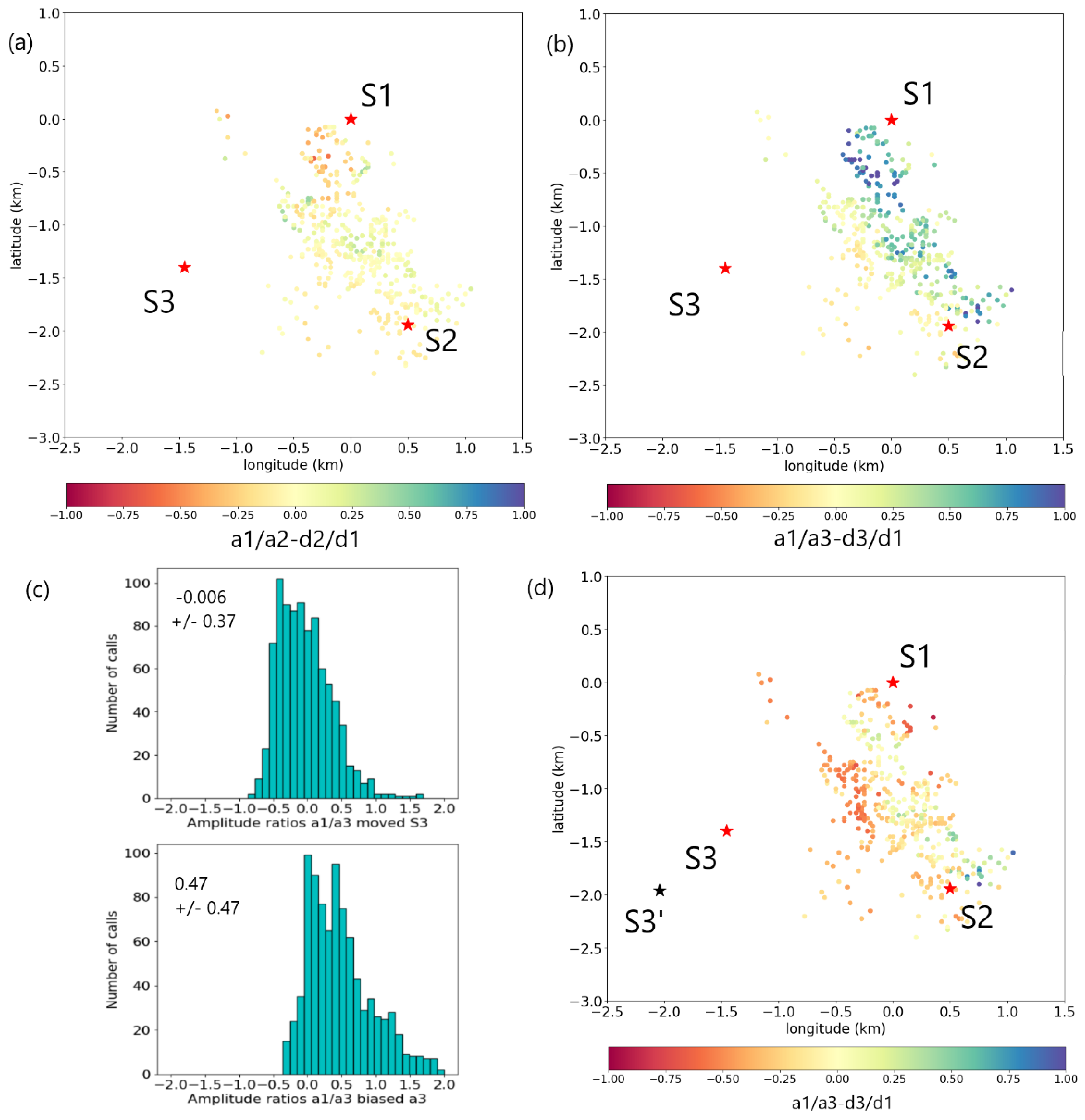
Figure 11 shows a spatial mapping of the residuals.
Figure 11a displays a1/a2-d2/d1 with low absolute values of the residuals, slightly negative values around S1, and slightly positive values midway between S1 and S2. The a1/a3-d3/d1 residuals show an apparent positive slope roughly from S3 to the S1-S2 line (
Figure 11b). A possible explanation for the discrepancies observed in the residuals in
Figure 11b is that the S3 hydrophone’s position is not correct and that it is located further away from the S1-S2 line than the coordinates used in this study indicate. Testing this hypothesis for a point located as shown on
Figure 11d as S3’, it is found that the constant bias is indeed removed from the distribution for point S3’ at coordinates (-2.04 km, -1.96 km, S3 hydrophone depth unchanged) on the S1-S3 line at a distance 1.4 times larger than the distance S1-S3.
The standard deviation of residuals after moving the location of S3 to S3’ is higher than when a constant bias correction on S3 amplitudes is applied. One also has to keep in mind that the calculation of the vocalization locations itself depends on the location of S3, and that these locations have not been updated in this work before re-calculating the residuals.
3.2. Taking Advantage of Dense Coverage Close to S1 and S2 to Estimate Depths
The amplitude bias between S1 and S2 seems to be minimal, and therefore it should be possible to compare amplitudes of received calls with locations directly above the hydrophones. In that case, the distance to the closest hydrophone is the depth difference between the vocalization and the hydrophone. Assuming that the calls have the same source levels, and that the depth of the source is similar, the relative amplitudes a1/a2 at S1 should be similar to the relative amplitudes a2/a1 at S2.
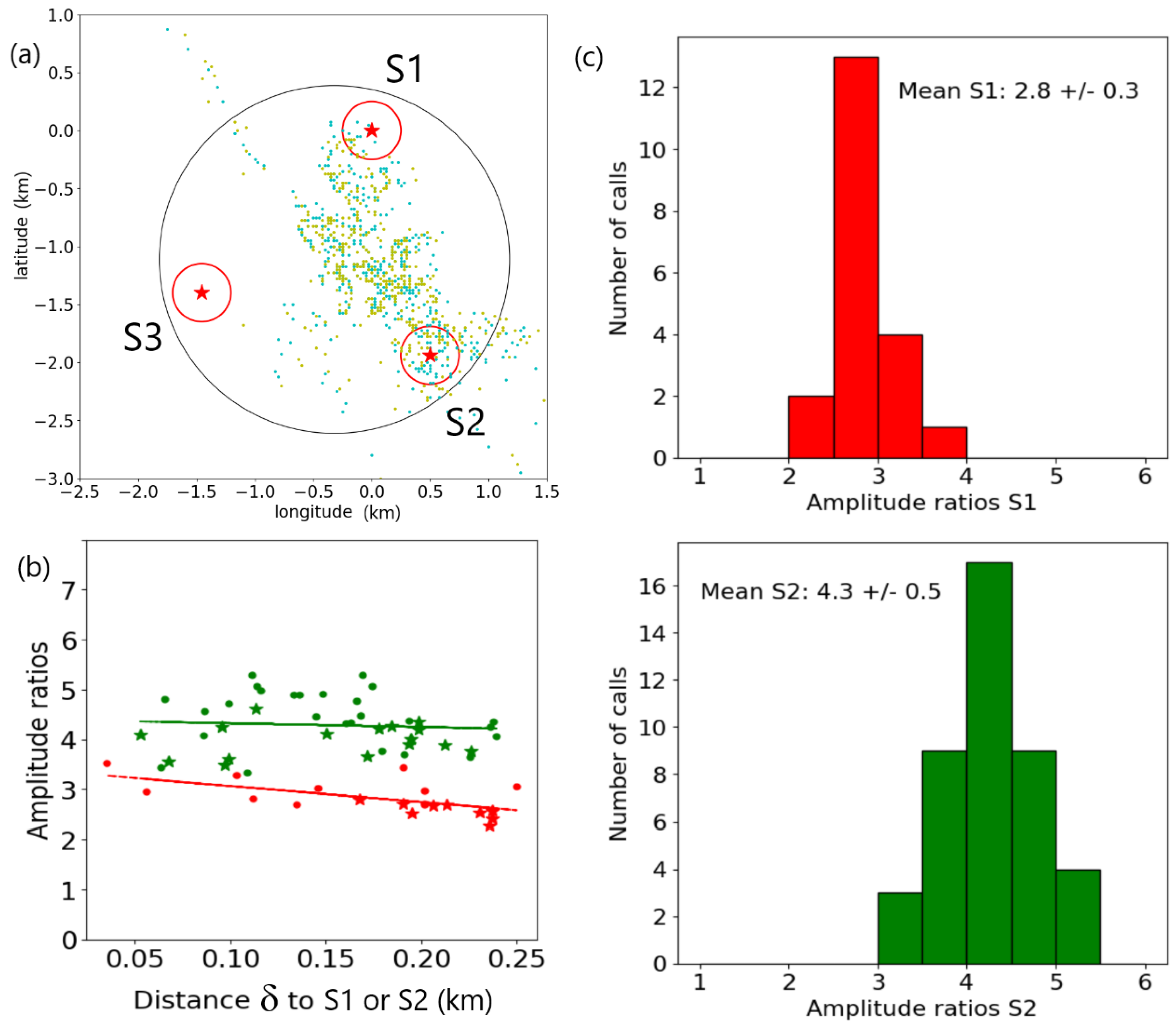
Figure 12a shows a map of call locations with a circle of 1.5 km in radius and circles of 250 m in radius around each of the three hydrophone locations.
The relative ratios a1/a2 are shown in red on
Figure 12b for the calls within the 250 m circle at S1, and a2/a1 are shown in green for the calls within the 250 m circle at S2, for a passage of the whale between 23:40 on the 19 February and 00:40 on the 20 February. The linear fit — a1/a2 = 3.39 – 3.21 δ with coefficient of determination r2 = 0.37 —extrapolates to a value of 3.39 at S1 and the linear fit —a1/a2 = 4.40 – 0.75 δ with coefficient of determination r2 = 0.006 — extrapolates to 4.40 at S2. A calls are marked as dots while B calls are marked as stars. When the values published in [
16] are used for the hydrophone depths, a ratio of:
would be expected for a whale depth, w=0m, at the surface, where h1 and h2 are the hydrophone depths of respectively S1 and S2 and D is the horizontal distance between them, which is 2 km. For w=20 m:
Figure 12b does indeed show that a ratio of
is measured close to S1, which is compatible with the above estimates using distances, and the linear fit extrapolates to a value of 3.39 at S1, from which a value of 135 m for the depth of vocalization of the whale can be derived. With the standard deviation of 0.3 for the ratio, the vocalization depth interval is 70 m to 190 m.
Conversely, at S2, the amplitude ratio would be expected to be:
This is to be compared with the measured value of at S2, and in this case, there is a discrepancy between the theoretical (from distance ratios) and observed values. The linear fit extrapolates to 4.40 at S2, meaning a value of 255 m for the depth. One possible explanation is that the vocalization depths is larger when it is close to S2. If a value of 0.5 is used for the standard deviation, the depth interval estimate is 190 m to 305 m.
Depths of the S1 and S2 hydrophones may have evolved since they were measured at respectively 750 m and 724m. For instance, assuming that S1 is now at a depth of 855 m, the values measured would account for a vocalization depth of 250 m when in the vicinity of S1 and S2.
4. Discussion
Waveforms originating from vocalizing whales recorded on the IMS hydro acoustics station HA11S have been presented and analysed for the possibility to localize the whales by TDOAs on each hydrophone in the station. The waveforms recorded for each whale call on each hydrophone are rendered complex by the presence of the water surface reflection and multiple water bottom reflections. This leads to issues with methods based purely on waveform cross-correlation such as the PMCC method [
25], when the vocalization happens close to the hydrophone. Some reflections are as energetic as the first, direct arrival, causing confusion as to which peak in the cross-correlation functions are to be used. The measurement of the amplitudes is also affected by the multiplicity of the arrivals, and perhaps a more sophisticated method than the one used in this study could be used to pick the amplitude of the first arrival with confidence, rather than assuming it will be the highest value of amplitude within a six second segment.
According to [
27], both triplets at HA11 were deployed around a seamount. It may not be a coincidence but rather directed by foraging around that seamount that initially, as shown on
Figure 8, the whale appears to head towards the seamount and to slow down around it.
The results shown in this paper are inconclusive regarding the depth of the vocalizations, partly because analysis of the amplitudes casts some doubt on the exact value of the hydrophone depths. It should be possible to extract the waveform of the original signal by assuming a spectral shape, pitch variation, and minimum phase for each of the A and B types of call, using wavelet deconvolution techniques from the seismic exploration industry [
26]. Waveform modeling using a method that identifies individual arrivals, such as ray methods, should then become feasible, leading to estimations of the reflection coefficients and more exact whale depths estimates.
The location results shown in this paper are relying on the exactitude of the location and depths of the hydrophones. It is likely that there are in fact differences of possibly a few tens of meters between the depths of the three hydrophones, as the mooring cable lengths were pre-established during deployment, but the exact water depth at which the hydrophones were dropped is likely to have deviated from the depth of the target locations, even though a very precise bathymetry was acquired before the deployment. Analysis of the amplitudes of the signals exploited in this work points to a possible underestimate of the depths of S1, and a possible need for either correcting the S3 location to a point further from S1 and S2 or taking into account a possible calibration correction of the hydrophone at S3. A simple study of a large number of horizontally propagating signals recorded at the triplet should be able to confirm or infirm a calibration issue. In analyzing the amplitude of the signals, the assumption was made that the source of sound is spherically symmetrical, with no azimutally or vertically dependent radiation pattern. It may be possible, in a more refined analysis, to use the direction of motion of the whale as a substitute for the position of the animal and detect any variation in the strength of the signal depending on the position of the receiver with respect to the whale and its front to rear axis.
An inversion problem using both amplitudes and delay residuals to estimate potential corrections to the hydrophone locations may be possible if a very large number of calls are collected. Early attempts at doing so using the locations derived from the delays and the residuals from the amplitudes yield unrealistically large corrections. It would also be beneficial to search the data for additional similar sequences, providing better coverage especially close to the S3 hydrophone.
Given the very close relationship between the locations and relative amplitudes of A and B calls, it is expected that either the source of the calls is a single animal, at least in contiguous periods of time, or if they are from two distinct animals, their relationship must be quite symbiotic. A different conclusion was reached by the authors of [
19], on very similar data from February 2019, also from HA11S. They concluded that A and B calls originated from two different animals. Our analysis could be repeated on the data set they used, with the addition of an analysis of the amplitudes in addition to the TDOAs.
5. Conclusions
The sequence of calls studied in this work has a long duration and the tracks followed by the whale allow for a good coverage of the area directly above the triplets. It was shown that using the amplitude ratios of the signal at two different hydrophones, when the source is in the near field, less than 1.5 km horizontally from the centre of the triplet, can be of interest. The amplitude ratios between S1 and S2 confirm that amplitudes follow the expected decay rule of being inversely proportional to the distance between source and receiver. This is however not the case for the amplitude ratios between S1 and S3. Several hypotheses may explain this, including that the relative location of S3 with respect to S1 and S2 needs to be corrected. Another possibility is that the amplitude radiation pattern of the calls is not isotropic, and there is a need to account for amplitudes decaying with the angle between the source-receiver line and the direction of propagation of the whale. Further collection of similar data with increased coverage may resolve which hypothesis explains the data best.
The A and B calls vocalization locations are very close to each other, and the variation from call to call of their relative amplitudes are extremely similar. This tends to show that either they originate with the same animal or from two animals with a very symbiotic relationship.
The estimated average swimming speed of the whale between A calls is 9.45 ± 7.05 km/h, and 9.57 ± 8.04 km/h between B calls. This is obtained when the cetacean is located less than 1.5 km from the center of the triplet, where locations and therefore distances swimmed are more accurately determined. The swim speed estimate is compatible with what is known about the maximum speed of 37 km/h (20 knots) for these cetaceans [
3].
A study of the residuals of observed amplitude ratios minus distance ratios and of the amplitude ratios when the whale is in the immediate proximity of hydrophones S1 on one hand and S2 on the other hand leads to the belief that corrections may be needed to the depths of the hydrophones.
As a general conclusion amplitude may be a source of information additional to the travel times provided that sensor locations are estimated within a few meters and that more is known about the radiation pattern of the acoustic sources.
Author Contributions
Conceptualization, R.L. and P.N..; methodology, R.L.; software, R.L.; formal analysis, R.L.; data curation, R.L.; writing—original draft preparation, R.L.; writing—review and editing, P.N.; All authors have read and agreed to the published version of the manuscript.
Funding
This research received no external funding
Data Availability Statement
The data from IMS hydroacoustic station HA11 is open available at the IRIS data center [
18]. The data from HA01 as shown on
Figure 1 can be obtained via the vDEC [
25] mechanism of the CTBTO.
Conflicts of Interest
The authors declare no conflicts of interest.
References
- CTBTO Web site www.ctbto.org (last accessed 12 November 2024).
- IMS map https://www.ctbto.org/sites/default/files/2024-10/IMS_Map_FRONT_BACK_AUGUST_2021_web2.pdf (last accessed 12 November 2024).
- International Whaling Commission. https://iwc.int/about-whales (last accessed 7 July 2024).
- Munk, W. H. (1974). “Sound channel in an exponentially stratified ocean with applications to SOFAR,” J. Acoust. Soc. Am. 55, 220–226. [CrossRef]
- Thode, Aaron. (2004). Tracking sperm whale (Physeter macrocephalus) dive profiles using a towed passive acoustic array. The Journal of the Acoustical Society of America. 116. 245-53. [CrossRef]
- Thode, A. M., Kim, K. H., Blackwell, S. B., Greene, C. R., Nations, C. S., McDonald, T. L., et al. (2012). Automated detection and localization of bowhead whale sounds in the presence of seismic airgun surveys. J. Acoust. Soc. Am. 131, 3726–3747. [CrossRef]
- Miksis-Olds, J. L., Harris, D. V., and Heaney, K. D. (2019a). “Comparison of estimated 20-Hz pulse fin whale source levels from the tropical Pacific and Eastern North Atlantic Oceans to other recorded populations,” J. Acoust. Soc. Am. 146(4), 2373–2384. [CrossRef]
- Harris, D. V., Miksis-Olds, J. L., Vernon, J. A., and Thomas, L. (2018). “Fin whale density and distribution estimation using acoustic bearings derived from sparse arrays,” J. Acoust. Soc. Am. 143(5), 2980–2993. [CrossRef]
- Balcazar, Naysa E., Joy S. Tripovich, Holger Klinck, Sharon L. Nieukirk, David K. Mellinger, Robert P. Dziak, Tracey L. Rogers, Calls reveal population structure of blue whales across the southeast Indian Ocean and the southwest Pacific Ocean, Journal of Mammalogy, Volume 96, Issue 6, 24 November 2015, Pages 1184–1193. [CrossRef]
- Gavrilov, A. N., McCauley, R. D., Salgado-Kent, C., Tripovich, J., & Burton, C. (2011). Vocal characteristics of pygmy blue whales and their change over time. The Journal of the Acoustical Society of America, 130(6), 3651-3660. [CrossRef]
- Gavrilov, A. N., & McCauley, R. D. (2013). Acoustic detection and long-term monitoring of pygmy blue whales over the continental slope in southwest Australia. The Journal of the Acoustical Society of America, 134(3), 2505-2513. [CrossRef]
- Le Bras, Ronan J., Heidi Kuzma, Victor Sucic, Götz Bokelmann; Observations and Bayesian location methodology of transient acoustic signals (likely blue whales) in the Indian Ocean, using a hydrophone triplet. J. Acoust. Soc. Am. 1 May 2016; 139 (5): 2656–2667. [CrossRef]
- Le Bras, Ronan J. and Peter Nielsen, (2017), Range estimates of whale signals recorded by triplets of hydrophones, AGU Fall Meeting. [CrossRef]
- Sirovic, A., Hildebrand, J. A., & Wiggins, S. (2007). Blue and fin whale call source levels and propagation range in the Southern Ocean. Journal of the Acoustical Society of America, 122(2), 1208-1215. https://escholarship.org/uc/item/8mr3c6vn. [CrossRef]
- Kuna, V. M., John L. Nábělek, Seismic crustal imaging using fin whale songs. Science 371,731-735(2021). [CrossRef]
- Stimpert, A.K., DeRuiter, S.L., Falcone, E.A. et al.. Sound production and associated behavior of tagged fin whales (Balaenoptera physalus) in the Southern California Bight. Anim Biotelemetry 3, 23 (2015). [CrossRef]
- Pereira, A., Danielle Harris, Peter Tyack, Luis Matias, 2020, On the use of the Lloyd's Mirror effect to infer the depth of vocalizing fin whales. J. Acoust. Soc. Am. 1 November 2020; 148 (5): 3086–3101. [CrossRef]
- Lloyd, Humphrey (1831). "On a New Case of Interference of the Rays of Light". The Transactions of the Royal Irish Academy. 17. Royal Irish Academy: 171–177. ISSN 0790-8113. JSTOR 30078788. Retrieved 2021-05-29.
- Zhu, J., Wen, L. (2024), Hydroacoustic study of fin whales around the Southern Wake Island: Type, vocal behavior, and temporal evolution from 2010 to 2022, J. Acoust. Soc. Am. 155, 3037–3050. [CrossRef]
- Various Institutions. (1965). International Miscellaneous Stations [Data set]. International Federation of Digital Seismograph Networks. [CrossRef]
- Lawrence, M., G. Haralabus, M. Zampolli, D. Metz, (2024). Comprehensive Nuclear-Test-Ban Treaty Organization, Vienna, (2024). The Comprehensive Nuclear-Test-Ban Treaty Hydroacoustic Network, in Kalinowski, M.B., Haralabus, G., Labak, P., Mialle, P., Sarid, E., Zampolli, M. (eds); Published by the Provisional Technical Secretariat of the Preparatory Commission for the Comprehensive Nuclear-Test-Ban Treaty Organization, Austria. https://www.ctbto.org/sites/default/files/2024-07/20240618-CTBTO%2025th%20Anniversary%20booklet%20Final%20HRes.pdf (last accessed 8/8/2024).
- Trnkoczy A. (2002), Understanding and parameter setting of STA/LTA trigger algorithm IASPEI New Manual of Seismological Observatory Practice 2 01 20 Bormann P. [CrossRef]
- Allen R.V. (1978), Automatic earthquake recognition and timing from single traces, Bull. seism. Soc. Am. 68 1521, 1532. [CrossRef]
- Le Bras, R. J., P. Mialle, N. Kushida, P. Bittner, P. Nielsen, (2024). Developments in Hydroacoustic Processing for Nuclear Test Explosion Monitoring, in Kalinowski, M.B., Haralabus, G., Labak, P., Mialle, P., Sarid, E., Zampolli, M. (eds); Published by the Provisional Technical Secretariat of the Preparatory Commission for the Comprehensive Nuclear-Test-Ban Treaty Organization, Austria. https://www.ctbto.org/sites/default/files/2024-07/20240618-CTBTO%2025th%20Anniversary%20booklet%20Final%20HRes.pdf (last accessed 8/8/2024).
- Cansi, Y. and Le Pichon, A. (2009) Infrasound Event Detection Using the Progressive Multi-Channel Correlation Algorithm. Handbook of Signal Processing in Acoustics, Springer, New York, 1425-1435. [CrossRef]
- Yi, Boyeon & Lee, Gwang & Kim, Han-Joon & Jou, Hyeong-Tae & Yoo, Dong-Geun & Ryu, Byong-Jae & Lee, Keumsuk. (2013). Comparison of wavelet estimation methods. Geosciences Journal. 17. [CrossRef]
- Braving storms. Constructing hydroacoustic station HA11 Wake Island. https://www.ctbto.org/news-and-events/news/braving-storms-constructing-hydroacoustic-station-ha11-wake-island (last accessed 22/7/2024).
- VDEC. https://www.ctbto.org/resources/for-researchers-experts/vdec (last accessed 10/7/2024).
Figure 1.
(a), (b), and (c) show two hours of unfiltered hydrophone data starting at 21:00 UTC on 19 February 2024 for, respectively, the S1, S2, and S3 hydrophones. At the one-hour mark approximately, frequent (approximately once every 25 seconds) impulsive signals are visible and increasing in amplitude towards the end of the section. The amplitudes are in mPa, and the horizontal lines are the -10, -20, 10, and 20 mPa levels. (d) Shows the basic geometry with the S1 hydrophone being the origin of the local coordinate system. S0 marks the center of the triplet and the arrow next to S3 shows how the back-azimuth is measured from North. The latitude and longitude differences are in kilometers. The absolute latitude and longitude of the S1 hydrophone are respectively 15.50827 degrees North and 166.700272 degrees East.
Figure 2.
Spectrograms of the first 30 minutes (a), and the last 30 minutes (b) of the two hours of waveforms for S2 shown on
Figure 1. An FFT length of 1024 points with 512 points overlap was used to compute the whole spectrogram over the 7200 s. The first 30 minutes and last 30 minutes were then windowed. The Nyquist frequency is 125 Hz. The frequency resolution is 0.244 Hz (512 intervals in [0-125] Hz) and the time resolution is 2.05 s.
Figure 3.
Illustration of the STA/LTA detection method on a 10 second interval with a single call at S1. (a) envelope of the first signal with red and blue time lines to show respectively the trigger-on and triger-off times. (b) STA/LTA function of the first signal. In addition to the time lines showing the trigger-on and trigger-off, the circle markers show their respective threshold values of 5 and 4 (c) STA/LTA of the envelope of the five-minute interval with fifteen calls. Each call is labelled A or B according to its center frequency. The red and blue horizontal dotted lines show the trigger-on and trigger-off thresholds.
Figure 4.
Traces S1, S2, and their crooscorrelation function CC12 for the call shown in
Figure 3. The zero on the time axis is the time of the pick on S1. The maximum of CC12 is 0.73 for a time shift of -0.23 s.
Figure 4.
Traces S1, S2, and their crooscorrelation function CC12 for the call shown in
Figure 3. The zero on the time axis is the time of the pick on S1. The maximum of CC12 is 0.73 for a time shift of -0.23 s.
Figure 5.
Panel (a) shows the results of picking TDOAs based on method 1 (cross-correlation), and panel (b) is based on method 2 (STA/LTA picks only). Panel (c) shows the result of improved method 2, obtained by adjusting (b) with cross-correlation values when TDOAs obtained with the two different methods are within a tenth of a second of each other. Red dots are the delays (d12) between S1 and S2, the green dots, the TDOAs (d31) between S1 and S3, and the blue dots are the TDOAs between S2 and S3 (d23). On the right of each panel is a histogram of the errors estimated from the difference between the measured TDOAs e=(d12+d23+d31) which should theoretically be zero.
is called the closure and is described in detail in [
25].
Figure 6.
(a) Illustration of the amplitude differences between A and B types of calls. The amplitude measures for type A is consistently higher than for type B. The amplitude scale is in mPa. (b) Shows the consistency of the relative amplitudes for types A and B, in this case amplitude at S1 divided by amplitude at S2.
Figure 7.
Panels (a) and (b) show the results of applying a crosscorrelation method on 5 s segments with 50% overlap, on time interval [18:20 - 21:00] UTC on 19 February 2024. Panels (c) and (d) are for interval [21:00 - 23:00] UTC. Panels (a) and (c) show the back-azimuth estimates when a threshold correlation value of 0.3 for at least one of the three cross-correlations is used. Panels (b) and (d) show the histograms of error estimates for the respective time intervals.
Figure 8.
Panel (a) is a map showing the location of all A calls (small green dots) detected during the two-hour interval shown on
Figure 1. Six of the calls are shown with larger yellow dots and labeled in minutes, corresponding to the detection time on S1 after 18:00 UTC on 19 February 2024, and show the progression of the whale from the northwest of the triplet to its center. The red stars are the locations of the hydrophones. Panel (b) to (d) are the surfaces of the time delay residuals at the time indicated. The yellow star shows the location of the minimum of the RMS of delay residuals for the three specific calls. Note that panels (b) to (d) show ten-kilometers squares centered on the yellow star.
Figure 9.
(a) Distances between consecutive calls of the same type based on locations derived from the TDOAs for the A and B calls. The red dots correspond to the A calls and the green dots to the B calls. The yellow line shows the distance from the B calls to the centre of the triplet. Since the A and B calls are close to each other, the line derived from the A calls would be very similar. The solid black indicates 1.5 km. (b) shows the histogram of estimated speed between two consecutive A calls when inside the 1.5 km line for the two different calls (c) shows the histograms of velocity estimates between consecutive B calls.
Figure 10.
Relative measured amplitudes a1/a2 (a) and a1/a3 (b) displayed as a function of time when the call location is within 1.5 km of the triplet centre. The scale is in minutes from 18:00 on 19 February 2024. For comparison, the distance ratios d2/d1 and d3/d1 are displayed on the same graphs. When a constant bias of 1.03 and 1.37 are applied to respectively a2 and a3, the graphs are displayed in (c) and (d). The histograms of the residuals (a1/a2-d2/d1) and (a1/a3-d3/d1) corresponding to each time series are shown to the right of each time series along with their mean and standard deviation.
Figure 11.
Spatial mapping of residuals a1/a2-d2/d1 (a) and a1/a3-d3/d1 (b). Note the higher amplitudes of the residuals in (b), which a plane sloping from the S1-S2 line towards S3 would fit. (c) Histograms of the a1/a3-d3/d1 residuals with original S3 (bottom) and moved S3’ (top). (d) Residuals a1/a3-d3/d1 when S3 is moved to S3’.
Figure 12.
(a) Map of all calls analyzed in the study. 597 A calls are in cyan, 600 B calls in yellow. The large circle is centered in the middle of the triplet and has a radius of 1.5 km. The small red circles are centered on each hydrophone and have a radius of 250 m. (b) Amplitude ratios a1/a2 in red, and a2/a1 in green, displayed as a function of distance for calls within 250 m of the hydrophones. (c) Histogram of the amplitude ratios a1/a2 for calls close to S1. (d) Histogram of the amplitude ratios a2/a1 for calls close to S2.
Table 1.
Basic geometry parameters for HA11S triplet. Water depth is 1174 m.
Table 1.
Basic geometry parameters for HA11S triplet. Water depth is 1174 m.
| Hydrophone |
Identifier |
Latitude
Longitude*
(decimal degree) |
Latitude
Longitude
(km from S1) |
Depth
(m) |
| H11S1 |
S1 |
18.50827
166.700272 |
0.000
0.000 |
739**
750*** |
| H11S2 |
S2 |
18.49082
166.705002 |
-1.939
0.498 |
739**
742*** |
| H11S3 |
S3 |
18.49568
166.686462 |
-1.399
-1.455 |
739**
724*** |
|
Disclaimer/Publisher’s Note: The statements, opinions and data contained in all publications are solely those of the individual author(s) and contributor(s) and not of MDPI and/or the editor(s). MDPI and/or the editor(s) disclaim responsibility for any injury to people or property resulting from any ideas, methods, instructions or products referred to in the content. |
© 2024 by the authors. Licensee MDPI, Basel, Switzerland. This article is an open access article distributed under the terms and conditions of the Creative Commons Attribution (CC BY) license (http://creativecommons.org/licenses/by/4.0/).