
Submitted:
26 April 2023
Posted:
03 May 2023
You are already at the latest version
Abstract
Semidiurnal tidal currents can exceed 5 ms−1 in Minas Passage, Bay of Fundy, where a tidal energy demonstration area has been designated to generate electricity using marine hydrokinetic turbines. The risk of harmful fish-turbine interaction cannot be dismissed for either migratory or local fish populations. Individuals belonging to several fish populations have been acoustically-tagged and monitored by using acoustic receivers moored within Minas Passage. Detection efficiency ρ is required as the first step to estimate probability of fish-turbine encounter. Moored Innovasea HR2 receivers and high residency (HR) tags were used to obtain detection efficiency ρ as a function of range and current speed, for near-seafloor signal paths within the tidal energy development area. Strong tidal currents moved moorings so HR tag signals, and their reflections from the sea surface, were used to measure ranges from tags to receivers. HR2 self-signals that reflected off the sea surface showed which moorings were displaced to lower and higher levels on the seafloor. Some of the range testing paths had anomalously low ρ which might be attributed to variable bathymetry blocking the line of sight signal path. Clear and blocked signal paths accord with mooring levels. Application of ρ is demonstrated for calculation of abundance, effective detection range, and detection-positive intervals. High residency signals were better detected than pulse position modulation (PPM) signals. Providing the presently obtained ρ applies to tagged fish that swim higher in the water column, there is a reasonable prospect that probability of fish-turbine encounter can be estimated by monitoring fish that carry HR tags.
Keywords:
detection efficiency
; effective detection range
; abundance
; tidal energy
; MHK turbine
; fish-turbine encounter
1. Introduction
The ocean is vast and largely opaque to human senses. Acoustic telemetry tags have been used in many ways to study the ecology and behaviour of fish. Strategically placed arrays of acoustic receivers can be used to observe and quantify migration [1,2,3] or demonstrate seasonal presence [4] and indicate species’ residency patterns [5,6]. With a sufficient density of acoustic receivers, localization can be achieved so that fish can be tracked with high resolution and their behavior studied within a small area [7,8,9]. Detection range experiments [10,11,12] quantify how efficiently acoustic tag transmissions are detected as a function of range and environmental conditions and such knowledge is fundamental for designing experiments to achieve all of the above.
Detection of an acoustic signal from a tagged fish indicates presence in some sense but has restricted value as an ecological variable. Ecology is usually measured and modelled in terms of variables like abundance; sometimes quantified in terms of the number individuals per unit area at some location [13]. Probability of detecting known signal transmissions as a function of range enables the effective detection area to be defined and so detection range experiments are, therefore, fundamental for converting detected signals from acoustically tagged fish into metrics for ecological interpretation.
Our motivation for undertaking detection range measurements is closely related to the quantification of abundance. Specifically, our ultimate goal is to quantify the probability that a fish belonging to some local population will encounter marine hydrokinetic (MHK) turbines [14,15] that are to be deployed at the Fundy Ocean Research Center for Energy tidal energy demonstration (TED) area in Minas Passage, Bay of Fundy, Canada (Figure 1).
Vertically-averaged tidal current can be in excess of 5 ms in the TED area and the associated power density is enticing for deployment of MHK turbines that convert tidal kinetic energy to electricity [16,17]. Large tidal range can result in about 60% of the water in Minas Basin flowing in and out through Minas Passage in a semidiurnal tidal cycle [18], so some fish that are commonly found in Minas Basin also pass through the TED area in Minas Passage [19]. Minas Passage is also the sole corridor for migratory diadomous fish populations that utilize Minas Basin and its associated freshwater tributaries for reproduction and rearing. Of the species of fish commonly found in Minas Basin [20], acoustic telemetry measurements made in Minas Passage have been reported for striped bass Morone saxatilis [4], Atlantic sturgeon Acipenser oxyrinchus [2], alewife Alosa pseudoharengus [3], and Atlantic salmon Salmo salar and American eel Anguilla rostrata [21]. Acoustic telemetry work continues on the above species as well as tomcod Microgadus tomcod, spiny dogfish Squalus acanthias and American shad A. sapidissima.
Fast current makes the TED area a difficult place to deploy scientific instruments and adversely affects acoustic telemetry [12,22,23]. Active acoustic measurements (echosounders) are also difficult to utilize [24,25] and have the added disadvantage of not being able to identify the species of a target. Since 2010, Innovasea VR2W receivers have been used in Minas Passage to monitor Atlantic sturgeon, striped bass and American eel that carried Innovasea acoustic tags that use pulse position modulation (PPM) of a 69 kHz carrier frequency [21]. Ambient sound level greatly increased when current was fast and PPM tags could only be detected at close range [12]. Furthermore, at small range, close proximity detection interference (CPDI) [11] causes further uncertainty for signal detection [12]. A 69 kHz PPM tag signal consists of eight 10 ms pulses spaced over a few seconds, so signals are transmitted infrequently because of the energy cost and the need to avoid interference by pulses originating from another tag. Few 69 kHz PPM signals can be transmitted before fast currents sweep a tagged fish beyond the detection range of a VR2W receiver so tagged fish were detected. This presents an impediment for estimating fish-turbine encounter probability because it is encounters at high current speeds that are of most interest.
Given the lower ambient sound level at higher frequencies [12], some of the tagging effort has shifted to using Innovasea 170 kHz high residency (HR) tags in recent years. HR tags encode information by abrupt phase changes within a 6 ms pulse, so HR signals can be transmitted much more frequently than PPM signals and many signals can reach a moored HR2 receiver before the current sweeps a tagged fish out of range. Alewives carrying HR tags that transmitted signals every 1-2 s were detected making many passes through Minas Passage on flood and ebb tides [3] even though the HR2 receiver array monitored only a small portion of the width of the passage. The apparent advantages of HR tags motivates the present measurements of their detection efficiency as a function of range and current speed.
HR technology has additional capabilities that were judged of potential use at our study site. The ability of HR2 receivers to separately identify a HR signal and its reflection allows calculation of range between a receiver and a transmitting tag that is at a known depth. HR signals reflected from the sea surface can also be used to monitor the depth of a HR2 receiver. These capabilities turned out to be crucial for measuring detection efficiency and the ability of the HR2 receiver to detect both 170 kHz HR and 180 kHz PPM signals enables a clear comparison of detection efficiency for those two signal types.
2. Materials and Methods
2.1. Moorings Design and Instrument Layout
Seven moorings were deployed for 32 d (9 April to 11 May 2021) on the volcanic plateau within the TED area (Figure 1). The line of moorings was orthogonal to the flood-tide current velocity. Each mooring consisted of a 240 kg anchor (a steel chain link) that was tethered by a 3 m riser chain to an acoustic release that was housed within the streamlined hull of a SUBS-Model A2 (Open Seas Instrumentation Inc.). Ideally, the moorings would hold HR2 receivers well clear of the seafloor to prevent blocking of transmission paths but strong, turbulent currents make severe mooring tilt inevitable using the available buoyancy-based, mooring technology [12]. The location was selected for its relatively flat and regular seafloor which was anticipated to minimize blocking of sound signals travelling between moored HR2 receivers.
Mooring deployment was during low tide with the intent of separating moorings by 50 m. Currents are never really slack in the TED area so navigation is difficult. Table 1 documents the research vessel position at the time each mooring was released overboard from the stern. The research vessel’s GPS was about 10 m forward of the drop position so acoustic methods must be used to check and refine estimates of mooring separation. HR tags were attached to the top of the SUBS tail fin at sites 1 and 7. HR tags transmitted 143 dB signals with 170 kHz HR signals set to a random delay interval of 1.8-2.2 s and 180 kHz PPM signals set to 15-25 s delay. Due to a miscommunication with the manufacturer, both of the HR tags turned off at about 1832 UTC on 23 Apr 2021, a little short of halfway through the experiment. It was intended that all HR2 receivers be set to transmit 143 dB HR signals within a random delay interval of 4-6 s, but the delay interval was mistakenly set to 25-35 s for site 3.
Every 10 minutes the HR2 receivers recorded water temperature and the tilt angle of the HR2 from vertical. 10 minute sampling is adequate when using water temperature to estimate sound speed but underresolves fluctuations in SUBS orientation. Nevertheless, in a statistical sense, the tilt measurements indicate whether or not a SUBS maintains streamlined orientation relative to the current.
2.2. Types of HR Signals that are Detected by a HR2 Receiver
A HR2 receiver records detected signals according to the time they are detected and their identity. Presently we define five types of HR signals that are detected by HR2 receivers. For a given purpose, detected signals may be useful or a hindrance depending upon their type.
Type HR are signals that travel along a direct path from some other source to the detecting HR2 receiver. The other source might be a tag or a different HR2. Type HR are signals that are transmitted from some other source but are reflected off the sea surface before reaching the detecting HR2.
Type HR is classified by Innovasea as a “SELF DET” and is a HR signal that a HR2 both transmits and records at the time of transmission. Type HR is when a HR2 receiver detects a reflection of its own HR transmission. HR signals are usually reflected from the sea surface but sometimes they are reflected from deeper objects nearby the mooring.
Rarely, the HR transmission can interact with a very nearby object in such a way as to create a signal with a fake identity. Remarkably, the transmitting HR2 will correctly record the identity and time at which the HR was transmitted and fractionally later will also record the time of arrival of the fake signal along with its fake identity. This will be called a HR signal. Very infrequently, the transmitting HR2 will detect such fake signals after they have been reflected from the sea surface. Sometimes the fake signal is detected by an HR2 that is different from that from which it originated.
2.3. Removal of Some HR for Estimating Detection Efficiency
Acoustic impedance is much greater in water than air so the sea surface reflects sound very well [26]. A HR signal that is detected by a HR2 receiver (but was not transmitted by that receiver) might have travelled a direct path from transmitter to receiver or it might have travelled a path corresponding to reflection from the sea surface. Sometimes the same transmitted signal will be detected twice, first the HR signal and a fraction of a second later the HR. In such circumstances the HR signals are easy to identify because the time lapse from the HR is very much less than the time lapse between successive transmissions (Table 1).
Let be the number of transmissions that were detected after travelling both a direct (d) and (∧) reflected (r) path, corresponding to detected signals. For estimating detection efficiency, we must remove the reflected signals that closely follow signals that travelled a direct path.
2.4. Removal of HR for Calculating Mooring Separation
HR signals (received after reflection from the sea surface) are troublesome if included in the data set used for synchronizing clocks on two HR2 receivers and measuring the distance between those receivers. Usually HR are also a hindrance when using an array of receivers to localize the position of a tagged fish, although they can also be valuable for such calculations providing special care is taken [27].
The total number of detected signals , from X transmisisons, can be written in a form that is relevant for calculating mooring separation
where is the number of transmissions that were detected after travelling a direct (d) path and (∧) were not (∼) detected after travelling a reflected (r) path. is the number of transmissions that were not detected after travelling a direct path but were detected after travelling a reflected path. transmissions were detected for both direct and reflected paths. As before, it is easy to remove the reflections that immediately follow detection of a direct-path signal so the the number of detected transmissions is
The undetected transmissions can be written so the total number of transmissions is
That leaves troublesome reflected signals within the detected signals which cannot be identified and removed before synchronizing clocks and calculating mooring separation. Let us, therefore, evaluate the extent to which those reflected signals are present.
Calculation of synchonization and separation first requires matching a short sequence of transmissions to a sequence of detections. Such matching is best achieved when the proportion of transmissions that are detected is large, i.e., is .
Signals travelling both reflected and direct paths suffer signal attenuation and distortion as they travel through the turbulent water volume and both must rise above the same ambient noise level to be detected. These things effect the probability of detecting a transmission in a way that is similar for both direct and reflected paths, perhaps more for reflected signals that transit a path that is significantly longer than the direct path. Reflected signals suffer additional distortion and scattering from a roughened sea surface which introduces a probability that an incident signal will be reflected sufficiently cleanly for the possibility of detection. Thus detection of reflected signals scales as relative to signals on a direct path. This suggests that scales as , scales as , and scales as . When is small and is large
and the troublesome reflections are rare.
2.5. HR2 Depth Relative to the Sea Surface
When a HR2 receiver detects a reflection HR of its own transmission HR then there is a high probability that that reflection was from the sea surface. In such circumstances the vertical distance is the speed of sound c multiplied by half the time lapse between when the HR signal was transmitted and when it was detected. Speed of sound was calculated following [28] by using temperature measured by the HR2, using hydrostatic pressure at half the mooring depth in Table 1, and by assuming ppt salinity. Previous measurements in Minas Passage indicated salinities in the range 30.5 to 32 ppt [29,30,31] with tidal excursion causing salinity to sometimes vary by as much as 1 ppt [30]. Current also influences sound wave propagation but signal paths are approximately orthogonal to the current so the effect is minimal.
Reflections from the sea surface give a gappy time series for the height of the water column above the HR2. For each day, at each site, a regression fit to tidal harmonics (M2, S2, N2, M4) was then used to obtain a daily averaged estimate of depth along with its 95% confidence interval.
2.6. HR2 Synchronization and Site Separation
By taking care to reference the HR2 to UTC soon before/after mooring deployment/recovery, much of the clock skew could be removed. It is then less computationally difficult to pattern-match a time-sequence of HR transmissions from one HR2 to a corresponding (possibly gappy) time-sequence of HR signals detected by a neighbouring HR2. Times at which signals are detected and transmitted enable more accurate synchronization and calculation of the separation between receivers.
Consider that HR2 receivers and are separated by some unknown range r and that there is an unknown clock offset so that at an instant when receiver records time the receiver records time . In order to calculate separation range r and time offset we write the travel-time equations for two signals. Receiver transmits signal i at time and receives signal i at time
where c is the speed of sound. Receiver transmits signal j at time and receives that signal at time
It is now trivial to solve the above equations for r
and
as functions of the transmission and reception times that the two receivers recorded for signals i and j. Current has minimal influence on the calculation of r because moorings are aligned across the current (Figure 1).
2.7. Separation Between Tags and HR2 Receivers
A first estimate of separations between moorings can be obtained from latitudes and longitudes in Table 1. Separations between HR tags and HR2 receivers were also calculated from the time lag between reception of a tag transmission travelling a direct path and a path that reflected from the sea surface. In order to make this calculation we assume that the HR2 receiver and the tag are at the same depth D below the seasurface. This amounts to synchronous signals being sent from two sources separated by in the vertical. For sufficiently large D this amounts to a large aperture. Using the Pythagorean identity, separation range r is then calculated as
This equation is a simplification of a calculation [27] for obtaining the range and depth of a harbour porpoise (Phocoena phocoena). Lag distance also varies with tidal elevation. Before applying (11), linear regression was used to remove tidal constituents (M2, S2, N2, M4) from .
2.8. Tidal Current and Significant Wave Height
The present study measures how detection efficiency varies as a function of vertically-averaged tidal currents computed from the finite volume coastal ocean model FVCOM [16,17,32]. For present purposes, tidal currents and surface elevation were computed and stored at 10 minute intervals at site latitudes and longitudes documented in Table 1. Modelled currents do not capture fluctuations associated with turbulent eddies but are otherwise representative of ADCP current measurements in the TED area [33].
Throughout this study, we will use s to denote the signed tidal current speed, so s is positive on the flood tide and negative on the ebb tide. Tidal elevation and significant wave height were measured north of the TED area (-64.4040, 45.3690).
3. Results
Measuring detection efficiency is not trivial in the TED area. Moorings may move, so range r between moorings must be measured throughout the study. Proper account must be taken of signals taking direct and reflected paths. Interpretation of signals transmitted over near-seafloor paths requires an assessment of vertical level for each mooring.
3.1. Transmission Between HR2 Receivers: Reflected Signals
Table 2 documents the number of HR transmissions from one site X and the number that were detected by a neighbouring site. The total number of detected HR signals was because there were transmissions that were detected after travelling both a direct and reflected path. For calculating range between sites, it is important that the reflections be removed. is typically 5-6% of the detected signals so failure to remove reflections can cause estimates of detection efficiency to exceed 1.
Detected transmissions,, include reflections that cannot be identified and removed but are troublesome for clock synchronization and calculating distance between HR2 receivers. The number of troublesome reflections that remain in the time series, , was calculated using (6) and values in Table 2 are consistent with scaling relationships (4). is small compared to , except for transmissions between sites 5 and 6. Nevertheless, we expect that and might might vary with environmental conditions so there may be times when is a smaller/larger proportion of than the averaged values in Table 2 might indicate.
Detection of reflections is expected to depend upon physical factors which vary with respect to time. It is not possible to construct a time series of reflected signals but it is possible to construct a time series of signals that were detected on both direct and reflected paths at each site. Stratifying this time series with respect to tidal elevation shows that reflections are 2.57 times more commonly detected when tidal elevation is below its 25th percentile than when it is above its 75th percentile. Stratifying this time series with respect to significant wave height shows that reflections are 5.15 times more commonly detected when significant wave height is below its 25th percentile than when it is above its 75th percentile.
3.2. Vertical Coordinate of the HR2 Receivers
Mooring locations and depths (Table 1) could only be roughly determined at time of deployment. Times at which an HR2 receiver transmits a self signal HR and then detects the reflection of that signal HR can be used to determine subsurface depth of the HR2 receiver. Subsurface depth of the HR2 receivers varies mostly due to the rise and fall of the tide (Figure 2) but at site 2 there is also a step-like depth increase for the latter half of the deployment. At site 4 some signals are reflected from a subsurface object (e.g. a boulder on the seafloor) that is initially about 10 m from the mooring, transitioning to about 12 m from the mooring and then disappearing during the latter part of the deployment. The inset in Figure 2 shows that reflections from the nearby object occur on the flood tide. This indicates horizontal mooring movement and forebodes that bathymetric features can interfere with signal reception.
Reflections of self signals from the sea surface give gappy time series of subsurface depth. Reflections that were obviously not from the sea surface were first removed. At each site, a regression fit to tidal harmonics (M2, S2, N2, M4) was then applied for each day of measurements so the fitted mean gives daily-averaged subsurface depth (Figure 3). In the latter portion of the deployment period, the mooring at site 2 slips downwards whereas the mooring at site 6 was dragged slightly upwards. Initially all HR2 receivers were m from the same level, but their levels varied by almost 2 m at the end of the experiment.
3.3. Separation of HR2 Receivers
Begin by eliminating the HR signals. Pattern matching time-sequences of transmissions to detections then gives values for travel-time equations (7) and (8). A pair of HR2 receivers can then be synchronized and their separation distance calculated using (10) and (9). An ensemble of many signals can be transmitted and received within a period that is sufficiently short for clock drift and site separation to have negligible change. Within an ensemble there are relatively few outliers and they are usually easy to recognize and remove. (Failing to remove the signals results in many more outliers and makes their removal difficult and tedious.) Averaging each ensemble gave separation ranges.
Figure 4 shows that for the first few days following deployment, there is some small variation in the separations between sites 2-3 and 5-4 but this is of little consequence for measuring detection efficiency. Left insets of Figure 4 show order 1 m changes in separation that are associated with tidal current, as though some mooring anchors were dragged slightly back and forth with the tide. These small changes of separation are too large to be attributed to changes in the speed of sound that might be caused by; tidal changes in hydrostatic pressure, errors in temperature measurements, or any physically pausible change in salinity.
Major variations in station separation (Figure 4) happened 26-28 April during spring tides (Figure 2) and were timed with the flood tide. This is consistent with the TED area having faster flood currents than ebb currents [16], so overall mooring displacement is most likely towards the east.
Separation between sites 2 and 5 changed little except for briefly moving a little closer together within the period 25-Apr to 2-May. In that same period, the right inset (Figure 4) shows transmissions from the HR2 at site 5 are reflected from a nearby object for a time interval that is coincident with sites 2 and 5 being a little closer together. Figure 3 indicates the site 2 mooring settling into deeper water. The most straightforward interpretation is that movement of site 5 accounts for most of the small change in separation between sites 2 and 5 whereas site 2 shuffled into a local hollow but otherwise was approximately stationary.
Given that site 5 moved little, site 6 moved by more than 100 m during 26-28 April 2021. Most likely sites 3, 4, and 6 all moved to an extent that was consequential for measuring detection range. Nevertheless, the separation ranges shown in Figure 4 are sufficient for estimating detection efficiency of signals transmitted by one HR2 and received by another — although different ranges apply at different times for the same pair of instruments.
The 240 kg anchor weight had been thought sufficient to prevent mooring movement on the volcanic plateau. Movement was greatest at site 6. Figure 5 shows HR2 measurements of the angle that the HR2 at site 6 was tilted from the vertical which corresponds to SUBS tilt from a streamlined orientation into the current. Such tilt measurements cannot resolve pitch from roll and yaw but they are indicative of lift and drag forces. When current speed is less than 2 ms the tilt is mostly in the range 10-15 (red bars in Figure 5) which is consistent with a stable lift-generating SUBS alignment. These low speed tilts occur on both the flood (45%) and ebb (55%) tides. Current speeds greater than 3 ms mostly happen (99%) on the flood tide. During fast, flood tides the tilt is distributed over a broad range, consistent with unstable alignment of the SUBS. In order to visualize the full variation of tilt, the distributions are also plotted on a log-linear scale in Figure 5. Large changes in tilt suggest large forces. The forces that the SUBS applies to the anchor are not just drag and lift, the fluctuating SUBS movement also causes inertial forces due to mass of the SUBS plus the virtual mass associated with the mass of seawater that the SUBS displaces [34].
On the flood tide, drifters accelerate to achieve higher speed as they pass over the volcanic plateau of the TED area (Figure 5). On average, the speed increment approaches 0.5 ms but individual drifter tracks show a good deal of variability that can be attributed to large-scale turbulent eddies. The flat, hard surface of the volcanic plateau may also make moorings vulnerable to movement. It is unclear whether mooring movement can be expected at sites that are not on the volcanic plateau.
3.4. Separation Ranges from Tags to HR2 Receivers
Ranges from tags (sites 1 and 7) to HR2 receivers were calculated from positions estimated at the time of deployment (second column of Table 3). Ranges from tags to HR2 receivers are only required up until 1832 23 Apr 2021 when the tags turned off. During that time, there was little movement of the HR2 moorings at sites 2 through 5 (Figure 4). Temperature measurements were interpolated to the time of each signal to obtain sound speed c and therefore the lag-distance . After removing tidal constituents, and subsurface depth m were substituted into (11) to obtain ranges in the third column of Table 3. Uncertainty in causes negligible error in the calculation of range r. On the other hand, varying D by m caused % change in range. Mooring separations obtained from are judged more reliable than those based upon estimates of drop position.
3.5. Detection Efficiency: Tag to HR2
Separations between HR tags and HR2 receivers were stable Table 3 while tags operated. No record is kept of when each tag transmitted but on average each tag is expected to transmit 300 times during a 10-minute interval. For each 10-minute time interval, there is a corresponding signed current speed s obtained from FVCOM. A specific tag-HR2 pair corresponds to a specific range and detected transmissions are then distributed as a function of s in 0.25 ms increments. The ratio of the number of signals detected to the number transmitted gives an estimate of detection efficiency for HR signals between a tag-HR2 pair.
The receiver at site 4 detected the tag at site 1 poorly compared to the tag at site 7 (Figure 6) even though both transmission paths had very similar ranges. Poor reception of signals travelling the 1,4 path might result from flood tide swinging the moorings so that the signal propagation path becomes blocked by a high spot in the bathymetry. High resolution bathymetry is available for the study area but although ranges between sites are accurately determined, the positions of the moorings are not. It was not possible, therefore, to test whether or not a particularly high spot existed on or near the 1,4 path. Given that the ultimate goal of such receiver arrays is to detect tagged fish that are usually well clear of the bottom, it was deemed appropriate to neglect results from the 1,4 path.
With two tags each detected by five receivers, there are 10 transmitter-receiver pairs at ranges marked by magenta line-ticks on the range axis of Figure 7. Ignoring the 1,4 path, Figure 7 shows contours of detection efficiency . It appears that the 1,5 and 1,3 paths might also have suffered some diminution of signal detection on the flood tide; less than that seen for the 1,4 path, but similar in form. Detection efficiency drops off rapidly when ms. Currents are faster on the flood tide, so estimates of detection efficiency are available for currents in the range ms.
3.6. Detection Efficiency: HR2 to HR2
HR2 moorings afford five receivers and five transmitters that transmitted and received HR signals throughout the study. The experiment was designed to measure two-way signal propagation along 10 transmission paths for a month. Figure 8 shows a time series of detection efficiency (calculated for 10-minute intervals) for HR signals transmitted between sites 4 and 5. Even for fast currents, while range is m. Mooring movement subsequently increases range to m and similarly fast currents cause a substantial reduction in although it always remained above 0. Results shown in Figure 8 contribute information near two ranges, and that is how they will be used for the calculation of .
Figure 4 shows separation for four pairs of sites, one of which is largely stable the others quite variable. Considering time series of separations between all HR2 sites, we identified 15 ranges that accommodated the majority of site-to-site separations to within a small uncertainty (Table 4). These ranges are marked with magenta on the vertical axis of Figure 9. Dotted magenta indicates ranges for which detection efficiency was poor compared with neighbouring ranges. Poor detection efficiency may result from the signal path being blocked by bathymetry. Figure 3 shows that site 6 was most elevated throughout the measurement period and this corresponds to site 6 featuring in most ranges for which detection efficiency was relatively high and the signal was deemed not to be blocked (Table 4).
It can be shown that poor performance at some ranges cannot be explained by statistical variability. Given the categorical nature of signal detection, the standard error of is where N is the number of independent measurements used to calculate . Estimates of are obtained from a great many instances and, except for the fastest flood/ebb currents, by averaging over many 10 minute intervals. Standard error is too small to explain the variability of that is seen in Figure 9. Rather, variation in is more likely associated with physical mechanisms (like mooring tilt and bathymetric blocking) or errors made while modelling currents. Given this balance of probabilities, it seems that measurements in Figure 9 that are judged to suffer from blocking should be discarded when calculating values for that are appropriate for detecting tagged fish that swim well clear of the seafloor.
Our experimental design did not adequately resolve how well signals are detected at ranges less than 40 m. Near 40 m range, Figure 8 indicates that detection probabilities greater than 0.4 are achievable on the fast flood current during a spring tide. This raises a prospect that, to a reasonable approximation, results shown in Figure 7 and Figure 9 might be made complete if detection efficiency can be estimated at very small range.
3.7. Detection Efficiency at Very Small Range
The Innovasea HR2 receiver delivers very few (if any) false detections that correspond to a specified HR tag identity. For example, the tags (ID’s 61676 and 61677) at sites 1 and 7 turned off 13.9 days into the present experiment. Before turning off, those tag ID’s were detected a total of 2.6 million times by the five HR2 receivers but they were not detected during the subsequent 18.1 days of the experiment.
A different type of false signal was found. The HR2 receiver (serial number 461550) at site 3 transmitted a HR signal with ID 62554 every 25-35 s. That HR2 detected a HR signal with ID 25202 a total of 2444 times and it was detected throughout the duration of the range test. (Innovasea confirmed that they had never manufactured a HR tag with that ID.) Analysis of times between consecutive HR transmissions corresponded to an underlying transmission interval in the range 25-35 s, as though the time series was a gappy version of signals being transmitted by the HR2 at site 3.
Of the 2444 HR signals, 2433 were detected at site 3 with a lag of s after that HR2 had transmitted its self signal. That lag corresponds to a transmission distance of 1.250 m. Our physical interpretation is that the HR2 was detecting a reverberation of its self-signal that was caused by the two flotation spheres housed within the SUBS. The other 11 times that HR was detected at site 3 it lagged the self signal by s which corresponded to detection after being reflected back from the sea surface.
For present purposes, regard the HR signal as having been transmitted 2444 times from site 3 and detected 2444 times at site 3. At greater range, HR was detected 503, 341, 267 and 27 times at sites 2, 4, 5 and 6, respectively. Blue bars in Figure 10 show the distribution of current when it is uniformly sampled though the experimental period. Current speed at the times when HR was detected at sites 2, 4, 5, and 6 had a different distribution (orange bars) which is consistent with detection at long range being much less likely when current speed is high. Current speeds at the times that HR was recorded at site 3 had a distribution (green bars) that was very similar to that for uniform sampling (blue). A fair interpretation is that, for current speeds in the TED area, very nearly all transmitted HR signals would be detected at 1.25 m range.
3.8. Detection Efficiency and Detection-Positive Interval
Detection efficiency has been modeled as a function . Temporal variation about this averaged formulation is expected because ambient sound level influences signal detection but ambient sound is only related to s in a statistically-averaged sense. It is, therefore, important to assess how might apply to the detection of the presence of a tagged fish during some interval that is sufficiently long so as to span many transmissions and sufficiently brief relative to tidal time scales so as to ensure that the same value of s applies.
Consider a tag that transmits every s that is present at a range r from an HR2 receiver when current is s. On average, the probability that a interval will be detection-positive is
is thus obtained as 1 minus the probability that none of the transmissions are detected. The calculation depends upon an assumption that detection of a transmitted signal does not influence the probability that the next transmission will be detected.
To test the applicability of (12), consider HR signals transmitted by the tag at site 7 and detected by the HR2 receiver at site 4 (Figure 6). The HR tag transmitted signals every s from a range of m for 13.86 days. Over that measurement period, each s interval was assessed detection-positive if one or more signals were detected and otherwise detection negative. Black crosses in Figure 11 show the fraction of detection-positive intervals for each speed bin. Detection efficiency for HR signal propagation between these sites can be substituted into (12) to also estimate the fraction of detection-positive s intervals (blue circles).
At low current speeds the detection efficiency is high and all intervals are detection positive, as expected. Lower detection efficiency at higher current speeds results in an appreciable fraction of the intervals being detection-negative and measurements show more detection negative intervals than expected from (12). This demonstrates that detection of a HR signal is not independent of whether the previous signal was detected. Obviously, if a given number of detected signals have a clumped distribution then there will be more detection-negative intervals than for a random distribution.
3.9. Detection Efficiency and Area of Effective Detection
Our present interest is to use near-seafloor HR2 receivers to detect tagged fish that are sufficiently clear of the seafloor so that the signal path from fish to moored HR2 receiver is unlikely to be blocked by bathymetric features. Removing these blocked paths (Table 4), and extrapolating to all signals detected at near-zero range, gives as contoured in Figure 12.
If a tagged fish is detected by a HR2 then provides a means to estimate the area within which the fish is expected to be located. Surrounding the position of the detecting HR2, an area of effective detection can be calculated (13) by integrating over the horizontal plane.
A is the area within which the tagged fish are effectively detected in a statistical sense. A might be conceptualized as an effective area within which the probability of detecting a tagged fish is 1 and outside of which the tagged fish would not be detected. Of course, no such sharp transitions exist so sometimes a tagged fish within A will not be detected and sometimes a tagged fish outside A will be detected.
Given tag signals from tagged fish where those signals are all detected throughout some time period T when current was s, then an estimate of abundance (number of tagged fish per unit area in the horizontal plane) can be obtained
where is the tag transmission interval. This is the elemental concept that can be used to convert signals detected by a receiver to an estimate of fish abundance.
Corresponding to the idea of an effective area for detecting tags, the range of effective detection is defined by
If is obtained from those transmission paths that do not appear to be blocked (Figure 12) then is as plotted by the blue line in Figure 13. Including blocked transmission paths in has the effect of diminishing R for fast flood currents (red line) but otherwise causes little change. Considering obtained from tag transmissions (Figure 9), and assuming that all signals are detected at very close range, gives larger effective range in slow currents (yellow line in Figure 13) but underestimates effective range in fast flood currents.
Having obtained the effective range, it is possible to describe the concept of effective detection area in a more quantitative way than above. Begin by calculating the inner area
by integrating only out to the effective radius R. The proportion of detected signals that originate within a physical space bounded by (within the effective area) is then given by the ratio . For present measurements of detection efficiency, this ratio is about 0.8 when current is slow. At higher current speeds, we might think of as being less step-like with respect to range which increases the likelihood that a detected fish may be outside the effective range.
3.10. Comparison of 170kHz-HR and 180kHz-PPM signals
Tags at sites 1 and 7 transmit more frequently than the HR2 receivers and there was little mooring movement during the period for which tags transmitted. Thus the detection of tag signals by the HR2 receivers provides the most reliable head-to-head comparison of detection efficiency for HR and PPM signals. Figure 7 shows detection efficiency for tag HR signals and the same procedure was used to obtain detection efficiency for tag PPM signals. The ratio of detection efficiencies (Figure 14) shows that HR signals are better detected than PPM signals, particularly at large range and in fast currents.
4. Discussion
Using tidal MHK turbines [14,15] to harvest kinetic energy [16] may offset some carbon emissions caused by Earth’s large human population relying on fossil fuel [35]. To address concern about fish-turbine encounters, acoustically-tagged fish have been monitored in Minas Passage since 2010. Most of that work used Innovasea 69 kHz PPM tags [2,4,6], but poor detection efficiency [12] has hindered reliable calculation of fish-turbine encounters when tidal currents are fast at the TED area in Minas Passage [36].
Present results show that 170 kHz HR signals are better detected than 180 kHz PPM signals and that this is especially so as range and current speeds increase. Also, HR signals do not suffer from CPDI [11] and can be transmitted much more frequently than PPM signals. Considering all these factors, HR tags will be more effective than PPM tags for studying fish-turbine encounters in Minas Passage. Recently, alewives with HR tags have been measured making multiple passes through the Minas Passage TED area [3] so presently obtained detection efficiency raises a prospect for reliable calculation of probability of alewife-turbine encounter.
Some illustrative progress on the MHK turbine encounter problem has been made using passive drifters [19]. While collision probability of drifters with MHK turbines at the TED area is a matter of concern for engineers and scientists, it does not directly translate to the fish-turbine encounter probability because the drifters were usually deployed on quasi-stable tracks that pass through the Minas Passage whereas fish might have quite different distributions depending on how they utilize their broader habitat [2,3,4,6]. Whereas a drifter track is well-resolved in space and time, the position of an acoustically tagged fish is entirely unknown except for those rare occasions when it is detected by a receiver. It is obvious when a tagged drifter passes by an array of receivers without being detected but there is no way to know how many times a tagged fish passes by without being detected.
Detection efficiency measurements expand the utility of detected signals from tagged fish. Given accurate detection efficiency and detected signals from tagged individuals belonging to a local population, equation (14) provides an estimate for abundance, . If those signals were detected by HR2 receivers at the TED area in Minas Passage, then is an estimate of the number of tagged individuals per unit area. Fish in the water column are expected to approximately move with the water when current speed is fast [19]. Given the vertical distributions of tagged fish [2,4], it is then straightforward to estimate the flux of tagged fish through a cross-current area that would, at some future time, be swept by the blades of a tidal MHK turbine. Probability that an individual belonging to a local population would encounter such a turbine can then be estimated by prorating according to the number of tagged individuals belonging to that population. Some fish might avoid the site when a MHK turbine is actually installed [37], while others may pass through a MHK turbine without being harmed [38], so the probability of encounter provides an upper limit on probability that an individual belonging to the population of interest may be harmed. Such metrics are directly relevant to population modelling [39] and thence to objective regulation of MHK turbines and fisheries.
The ability of the HR2 receiver to identify and record HR signals in quick succession showed that the probability was typically that a received pulse followed a direct path as opposed to being reflected from the sea surface. Probability of detecting a PPM signal depends upon the reception of 8 direct-path pulses without corruption by a reflected pulse. Making the physically plausible assumption that 69 kHz PPM pulses are reflected similarly to 170 kHz HR pulses, the probability of a PPM signal being corrupted by a reflected pulse is which is consistent with CPDI [11,12] being caused by pulses reflected from the sea surface. This was not unexpected because seawater has much greater acoustic impedance than air [26] and non-breaking surface waves are characterized by broad troughs and crests with maximum steepness less than 1/7 [40]. Other high frequency sound pulses have previously been observed to reflect from the sea surface with relatively little distortion compared to the highly scattered signals that reflect off the seafloor [27]. Furthermore, the present work demonstrated that the probability of receiving a reflected signal decreases with increasing significant wave height; a result that mechanistically supports an observation by others of low CPDI for an experiment conducted in choppy waters [11].
Careful account must be taken of reflected HR signals in order to ensure that the same signal is not counted twice when measuring detection efficiency. With respect to signals received from a tagged fish, there is no way to know whether an isolated signal travelled a direct or reflected path. Arguably this does not matter for measuring detection efficiency because both instances represent a single detection for a single transmitted signal. While reflected signals may not warrant mention for acoustic localization in very shallow water [9], the present work demonstrates that they matter when the tag is at greater depth because the source-to-receiver travel time of a reflected signal becomes quite different from that taking the direct path. Sometimes that difference can be useful for localization [27] but it is usually a hindrance. The present work found that most reflected signals could be identified and removed because they closely followed a signal taking a direct path.
Provided that HR2 moorings are within range of one and other, it may be possible to calibrate for the times that tagged fish are detected. When tagged fish are detected, concurrent measurement of might refine the estimate of area of effective detection and thus abundance. Alternatively, when tagged fish are not detected we can discern whether this might be due to a poorly performing HR2 receiver. A poorly performing HR2 receiver might also be indicated if it detects few reflections of its self signal compared to neighboring receivers. Separation of moorings can also be measured as a test that moorings have remained in place while fish are being monitored. Similarly, it is easy to monitor instrument depth when a HR2 receiver detects a reflection of its own HR signal. Where bathymetry is highly variable — as it is south of the TED area — such depth monitoring might indicate a HR2 mooring has slipped into a crevace. All these matters are of concern for accurate interpretation of measurements made in Minas Passage, where the available technology is pushed right to the edge of its capability.
Available mooring systems only enabled tags and receivers to be placed near the seafloor whereas tagged fish that we study usually swim well clear of the seafloor when they are in Minas Passage [2,4,41]. The range test could only measure signal paths that travelled from a near seafloor source to a near seafloor receiver. A 170 kHz sound wave has wavelength mm and so little energy can be expected to diffract around a much bigger object that obstructs the direct path from transmitter to receiver. Ray theory applies and there is an acoustic shadow zone behind the object [42]. Such blocking is not representative for detection of tagged fish that swim higher in the water column, so we presently consider it to be a source of error for the measurement of . For that reason, measurements from some signal paths were discarded because comparison with other paths of similar length made it obvious that signals were blocked by obstacles on the seafloor (Table 4). This procedure can remove the most obvious errors but it cannot ensure that those paths that remained did not, themselves, suffer from some degree of signal blocking, especially when fast currents tilt the mooring line [12]. Given that is of most interest in fast currents, it is necessary to resolve the possibility of such systematic error in order to calculate probabilities of encounter with confidence.
To confirm that the present measurements of HR detection efficiency apply for a tagged fish, measurements can been made by suspending tags beneath a drifter that passes over a receiver array. It is logistically difficult to use drifting tags to measure for all current speeds and ranges, but quasi-stable trajectories [19] do pass through Minas Passage when current is fast and thereby provide a means to test the applicability of present measurements of under conditions of concern. Consider a tagged-drifter (or tagged-fish) that transmits with interval and moves at speed past a fixed HR2 mooring. The number of signals that are expected to be detected can be calculated by integrating over the path taken by the drifter and multiplying by the number of signals transmitted along the path. Whereas the path of a tagged fish is not known, GPS measurements can accurately give the path of a drifter that carries tags. If our estimates of are accurate, should be comparable with the number of detections that are observed when the drifter passes by a receiver. Appropriate drifter measurements will be reported shortly [43].
5. Conclusions
- In fast tidal currents it is most advantageous for an array of HR2 receivers to be spaced so each HR2 can detect signals from its neighbours.
- Detection efficiency is variable over short intervals and values are not independent from one interval to the next.
- The concept of effective detection area has been introduced and can be calculated from detection efficiency. Effective detection area enables detected signals to be converted to an estimate of the abundance of tagged fish.
- Interpreting monitoring measurements in terms of fish-turbine encounter probability [36] has been held back for lack of confidence in previous estimates of at the TED area. Providing drifter measurements [43] confirm the present estimates of , there is every prospect of reliably calculating fish-turbine encounter probability [44] for a few of the many species of fish that are found in Minas Passage [20].
Author Contributions
Conceptualization, B.S., C.B. and D.H.; methodology, B.S. and D.H.; software, B.S.; formal analysis, B.S.; resources, B.S. and D.H.; data curation, B.S.; writing—original draft preparation, B.S.; writing—review and editing, B.S., C.B., L.M. and D.H.; visualization, B.S.; project administration, D.H.; funding acquisition, D.H. and B.S. All authors have read and agreed to the published version of the manuscript.
Funding
This research was funded by Natural Resources Canada (award ERPP-RA-07).
Data Availability Statement
The data sets analyzed during the current study are available from the corresponding author on reasonable request.
Acknowledgments
Jessica Douglas and Dylan DeGrace assisted with field work. Moorings were deployed and recovered with the assistance of Mike Huntley and the crew of the Nova Endeavour.
Conflicts of Interest
The authors declare no conflict of interest. The funders had no role in the design of the study; in the collection, analyses, or interpretation of data; in the writing of the manuscript; or in the decision to publish the results.
Abbreviations
The following abbreviations are used in this manuscript:
| FORCE | Fundy Ocean Research Centre for Energy |
| TED | Tidal Energy Demonstration |
| PPM | Pulse Position Modulation |
| HR | High Residency |
| HR2 | High residence receiver |
| CPDI | Close Proximity Detection Interference |
| FVCOM | Finite-Volume Coastal Ocean Model |
| GPS | Global Positioning System |
| UTC | Coordinated Universal Time |
| ADCP | Acoustic Doppler Current Profiler |
References
- Chavarie, L.; Honkanen, H.M.; Newton, M.; Lilly, J.M.; Greetham, H.R.; Adams, C.E. The benefits of merging passive and active tracking approaches: New insights into riverine migration by salmonid smolts. Freshwater Ecology 2022, 13, e4045. [Google Scholar] [CrossRef]
- Stokesbury, M.J.W.; Logan-Chesney, L.M.; McLean, M.F.; Buhariwalla, F.F.; Redden, A.M.; Beardsall, J.W.; Broome, J.; Dadswell, M.J. Atlantic sturgeon spatial and temporal distribution in Minas Passage, Nova Scotia: a region of future tidal power extraction. PLoS One 2016, 11. [Google Scholar] [CrossRef]
- Tsitrin, E.; Sanderson, B.G.; McLean, M.F.; Gibson, A.J.F.; Hardie, D.C.; Stokesbury, M.J.W. Migration and apparent survival of postspawning alewife (Alosa pseudoharengus) in Minas Basin, Bay of Fundy. Animal Biotelemetry 2022, 10. [Google Scholar] [CrossRef]
- Keyser, F.; Redden, A.M.; Sanderson, B.G. Winter presence and temperature-related diel vertical migration of Striped Bass Morone saxatilis in an extreme high flow passage in the inner Bay of Fundy. Canadian Journal of Fisheries and Aquatic Sciences 2016, 73, 1777–1786. [Google Scholar] [CrossRef]
- Kessel, S.; Hussey, N.; Crawford, R.; Yurkowski, D.; O’Neill, C.; Fisk, A. Distinct patterns of arctic cod (boreogadus saida) presence and absence in a shallow high arctic embayment, revealed across open-water and ice-covered periods through acoustic telemetry. Polar Biology 2009, 39, 1057–1068. [Google Scholar] [CrossRef]
- Keyser, F.M. Patterns in the movement and distribution of striped bass (Morone saxatilis) in Minas Basin and Minas Passage. MSc thesis, Acadia University, Department of Biology, 2015.
- Martins, E.G.; Gutowsky, L.F.G.; Harrison, P.M.; Mills Flemming, J.E.; Jonsen, I.D.; Zhu, D.Z.; Leake, A.; Patterson, D.A.; Power, M.; Cooke, S.J. Behavioral attributes of turbine entrainment risk for adult resident fish revealed by acoustic telemetry and state-space modeling. Animal Biotelemetry 2014, 2. Available online: http://www.animalbiotelemetry.com/content/2/1/13. [CrossRef]
- McLean, M.F.; Simpfendorfer, C.A.; Heupel, M.R.; Dadswell, M.J.; Stokesbury, M.J.W. Diversity of behavioural patterns displayed by a summer feeding aggregation of Atlantic sturgeon in the intertidal region of Minas Basin, Bay of Fundy, Canada. Mar. Ecol. Prog. Ser. 2014, 59–69. [Google Scholar] [CrossRef]
- Guzzo, M.M.; Van Leeuwen, T.E.; Hollins, J.; Koeck, B.; Newton, M.; Webber, D.M.; Smith, F.I.; Bailey, D.M.; Killen, S.S. Field testing a novel high residence positioning system for monitoring the fine-scale movements of aquatic organisms. Methods in Ecology and Evolution 2018, 9, 1478–1488. [Google Scholar] [CrossRef] [PubMed]
- Kessel, S.T.; Cooke, S.T.; Heupel, M.R.; Hussey, N.E.; Simpfendor, C.A.; Vagle, S.; Fisk, A.T. A review of detection range testing in aquatic passive acoustic telemetry studies. Rev Fish Biol Fisheries 2014, 24, 199–218. [Google Scholar] [CrossRef]
- Kessel, S.T.; Hussey, N.E.; Webber, D.M.; Gruber, S.H.; Young, J.M.; Smale, M.J.; Fisk, A.T. Close proximity detection interference with acoustic telemetry: the importance of considering tag power output in low ambient noise environments. Animal Biotelemetry 2015, 3. [Google Scholar] [CrossRef]
- Sanderson, B.G.; Buhariwalla, C.; Adams, M.; Broome, J.; Stokesbury, M.; Redden, A.M. Quantifying detection range of acoustic tags for probability of fish encountering MHK devices. In Proceedings of the 12th European Wave and Tidal Energy Conference, Cork, Ireland, 27 Aug-1st Sept 2017. [Google Scholar]
- Krebs, C.J. ; Ecology: The Experimental Analysis of Distribution and Abundance, 6th ed.; Pearson Benjamin Cummings, San Francisco, 2009.
- Jeffcoate, P.; McDowell, J. Performance of PLAT-I, a floating tidal energy platform for inshore applications. In Proceedings of the 12th European Wave and Tidal Energy Conference 27th Aug -1st Sept 2017, Cork, Ireland.
- Murray, J. Evolution of a solution for low cost tidal stream energy. Journal of Ocean Technology. 2021, 16(1), 1–8. [Google Scholar]
- Karsten, R.; McMillan, J.; Lickley, M.; Haynes, R. Assessment of tidal current energy in the Minas Passage, Bay of Fundy. Journal of Power and Energy 2008, 222(A3), 289–297. [Google Scholar] [CrossRef]
- Karsten, R. An assessment of the potential of tidal power from Minas Passage, Bay of Fundy, using three-dimensional models. In Proceedings of the ASME 2001 30th International Conference on Ocean, Offshore and Arctic Engineering, OMEA2011-49249, Rotterdam, Netherlands; 2011. [Google Scholar]
- Sanderson, B.G.; Redden, A.M. Perspective on the risk that sediment-laden ice poses to in-stream tidal turbines in Minas Passage, Bay of Fundy. International Journal of Marine Energy 2015, 10, 52–69. [Google Scholar] [CrossRef]
- Sanderson, B.G.; Stokesbury, M.J.W.; Redden, A.M. Using trajectories through a tidal energy development site in the Bay of Fundy to study interaction of renewable energy with fish. Journal of Ocean Technology 2021, 16(1), 50–70. [Google Scholar]
- Dadswell, M J; Spares, A D; Porter, E; Porter, D. Diversity, abundance and size structure of fishes and invertebreates captured by an intertidal fishing weir at Bramber, Minas Basin, Nove Scotia. In Proceedings of the Nova Scotia Institute of Science, Volume 50, Number 2, 2020, 283-318.
- Redden, A.M.; Stokesbury, M.J.W.; Broome, J.E.; Keyser, F.M.; Gibson, A.J.F.; Halfyard, E.A.; McLean, M.F.; Bradford, R.; Dadswell, M.J.; Sanderson, B.; Karsten, R. Acoustic tracking of fish movements in the Minas Passage and FORCE Demonstration Area: Pre-turbine Baseline Studies (2011-2013) (2014). Available online: https://tethys.pnnl.gov/publications/acoustic-tracking-fish-movements-minas-passage-force-demonstration- area-pre-turbine (accessed on 19 November 2022).
- Adams, M.; Sanderson, B.G.; Redden, A.M. Comparison of co-deployed drifting passive acoustic monitoring tools at a high flow tidal site: C-pods and icListenHF hydrophones. Journal of Ocean Technology 2019, 14, 61–83. Available online: https://www.thejot.net/archive-issues/.
- Tollit, D.; Joy, R.; Wood, J.; Redden, A.; Booth, C.; Boucher, T.; Porskamp, P.; Oldreive, M. Baseline presence of and effects of tidal turbine installation and operations on harbor porpoise in Minas Passage, Bay of Fundy, Canada. Journal of Ocean Technology 2019, 14, 24–48. Available online: https://www.thejot.net/archive-issues/.
- Viehman, H.; Boucher, T.; Redden, A.M. Winter and summer differences in probability of fish encounter (spatial overlap) with MHK devices. In: Committee, E.T. (ed.) Proceedings of the 12th European Wave and Tidal Energy Conference, 27 Aug-1 Sept 2017, Cork, Ireland (2017).
- Viehman, H.A.; Hasselman, D.J.; Douglas, J.; Boucher, T. The ups and downs of using active acoustic technologies to study fish at tidal energy sites. Frontiers of Marine Science, 2022, 9. [Google Scholar] [CrossRef]
- Lighthill, J. ; Waves in Fluids. Cambridge University Press, Cambridge, 1980.
- Sanderson, B.G.; Adams, M.J.; Redden, A.M. Using reflected clicks to monitor range and depth of Atlantic harbour porpoise. Journal of Ocean Technology 2019, 14, 85–100. Available online: https://www.thejot.net/archive-issues/.
- Mackenzie, K.V. Discussion of sea water sound-speed determinations. The Journal of the Acoustical Society of America 1981, 70, 801–806. [Google Scholar] [CrossRef]
- Bousfield, E.L.; Leim, A.H. The fauna of Minas Basin and Minas Channel. National Museum of Canada Bulletin 1959, 166, 1–30. [Google Scholar]
- Oceans Ltd: Appendix 5: Currents in Minas Basin (2010). Available online: https://fundyforce.ca/document-collection/environmental-assessment-2009 (accessed on 18 November 2022).
- Stewart: Oceanographic measurements — salinity, temperature, suspended sediment & turbidity, Minas Passage Study Site (2010). Available online: https://fundyforce.ca/document-collection/ (accessed on 18 November 2022).
- Chen, C.; Beardsley, R.C.; and Cowles, G. An Unstructured-Grid, Finite-Volume Coastal Ocean Model (FVCOM) System. Oceanography, 2006, 19, 78–89. [Google Scholar] [CrossRef]
- Passage and Minas Basin (2011). 2022. Available online: https://fundyforce.ca/document-collection/assessment-of-the-potential-of- tidal-power-from-minas-passage-and-minas-basin (accessed on 18 November 2022).
- Lighthill, J. ; An Informal Introduction to Theoretical Fluid Mechanics. Oxford University Press, Oxford, 1986.
- May, R.M. Ecological science and tomorrow’s world. Philosphical Transactions of the Royal Society B 2010, 365, 41–47. [Google Scholar] [CrossRef] [PubMed]
- Sanderson, B.G.; Redden, A.M. Use of fish tracking data to model striped bass turbine encounter probability in Minas Passage (2016). Available online: https://oera.ca/research-portal (accessed on 19 November 2022).
- Viehman, H.A.; Zydlewski, G.B. Fish interactions with a commercial-scale tidal energy device in the natural environment. Estuaries and Coasts 2015, 38 (Suppl 1), 214–252. [Google Scholar] [CrossRef]
- Amaral, S.V.; Bevelhimer, M.S.; Cada, G.F.; Giza, D.J.; Jacobson, P.T.; McMahon, B.J.; Pracheil, B.M. Evaluation of behavior and survival of fish exposed to an axial-flow hydrokinetic turbine. North American Journal of Fisheries Management 2015, 35, 97–113. [Google Scholar] [CrossRef]
- Gibson, A.J.F.; Myers, R.A. A statistical, age-structured, life history based, stock assessment model for anadromous alosa. In: Limburg, K.E., Waldman, J.R. (eds.) Biodiversity and Conservation of Shads Worldwide, pp. 275–283. 2003. [Google Scholar]
- LeBlond, P.H.; Mysak, L.A. Waves in the Ocean. Elsevier, New York, 1978.
- Renkawitz, M.D.; Sheehan, T.F.; Goulette, G.S. Swimming depth, behavior, and survival of Atlantic salmon postsmolts in Penobscot Bay, Maine. Transactions of the American Fisheries Society 2012, 141, 1219–1229. [Google Scholar] [CrossRef]
- Morse, P.M.; Ingard, K.U. Theoretical Acoustics. McGraw-Hill, New York, 1968.
- Sanderson, B.G.; Hasselman, D.J. Using drifters equipped with acoustic tags to verify the utility of detection efficiency measurements for estimating probability of fish-turbine encounter. J. Mar. Sci. Eng. Submitted.
- Sanderson, B.G.; Karsten, R.; Solda, C.; Hardie, D.C.; Hasselman, D.J. Probability of Atlantic salmon post-smolts encountering a tidal turbine installation in Minas Passage, Bay of Fundy. J. Mar. Sci. Eng. Submitted.
Figure 1.
Location of the mooring array on a flat volcanic plateau within the TED area on the northern side of Minas Passage, Bay of Fundy, Nova Scotia. The present study used seven moorings that are numbered from south to north. Depth contours are labelled in 5 m intervals.
Figure 1.
Location of the mooring array on a flat volcanic plateau within the TED area on the northern side of Minas Passage, Bay of Fundy, Nova Scotia. The present study used seven moorings that are numbered from south to north. Depth contours are labelled in 5 m intervals.
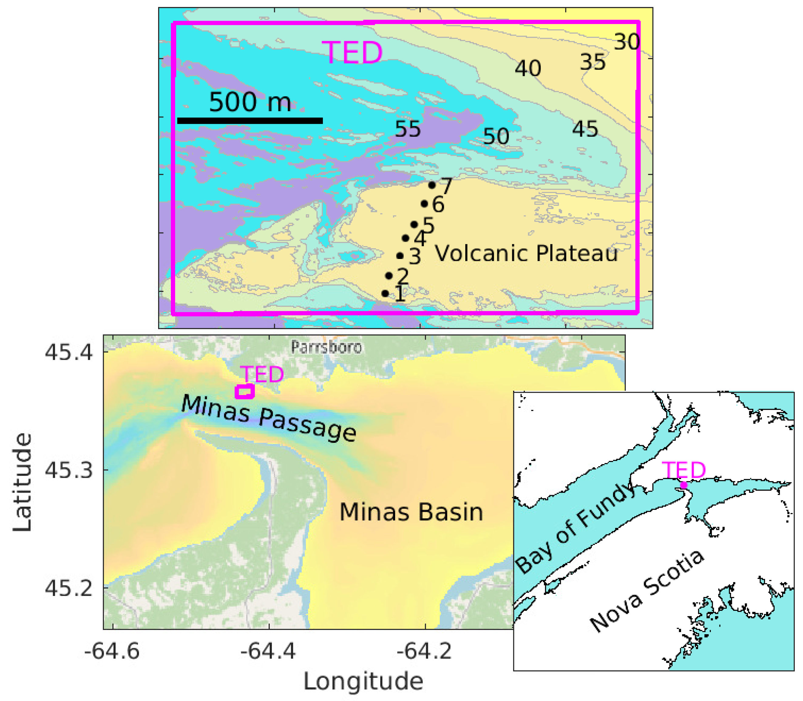
Figure 2.
Subsurface depth of the HR2 obtained from HR signals and their reflection from the sea surface.
Figure 2.
Subsurface depth of the HR2 obtained from HR signals and their reflection from the sea surface.
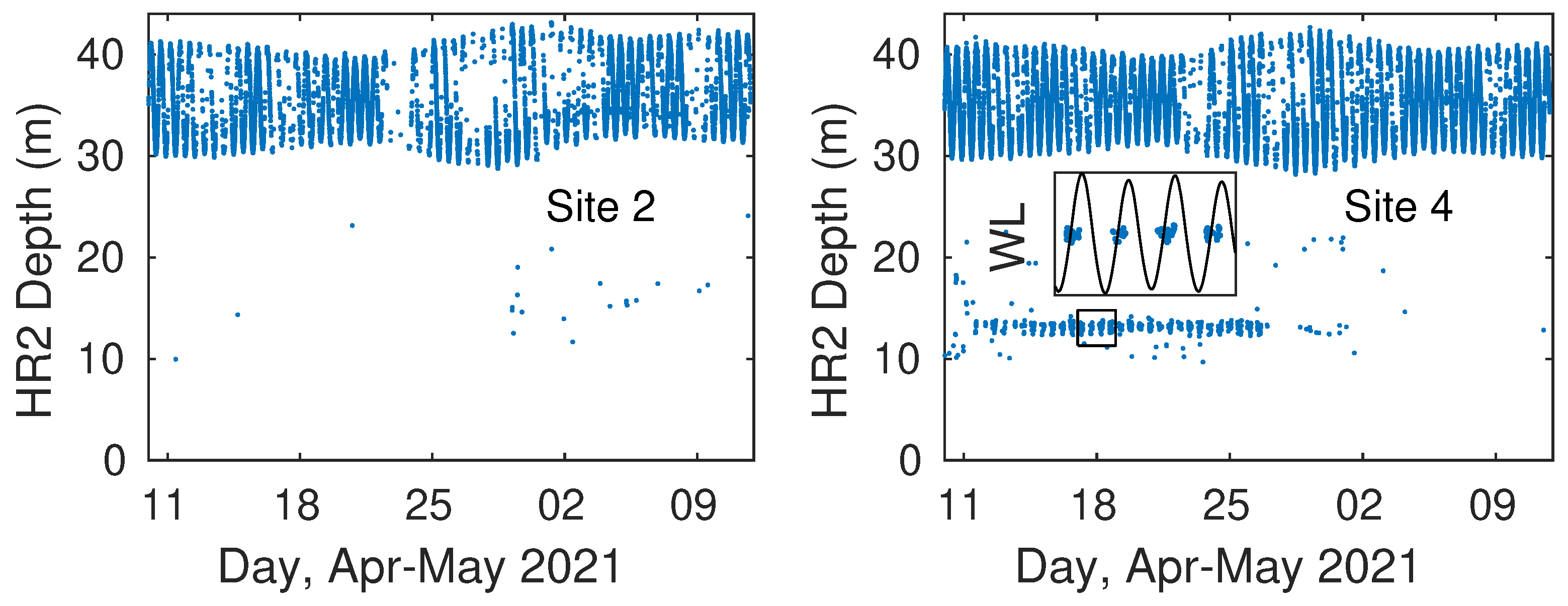
Figure 3.
Daily-averaged depths of the HR2 receivers. Vertical wiskers indicate the 95% confidence interval.
Figure 3.
Daily-averaged depths of the HR2 receivers. Vertical wiskers indicate the 95% confidence interval.
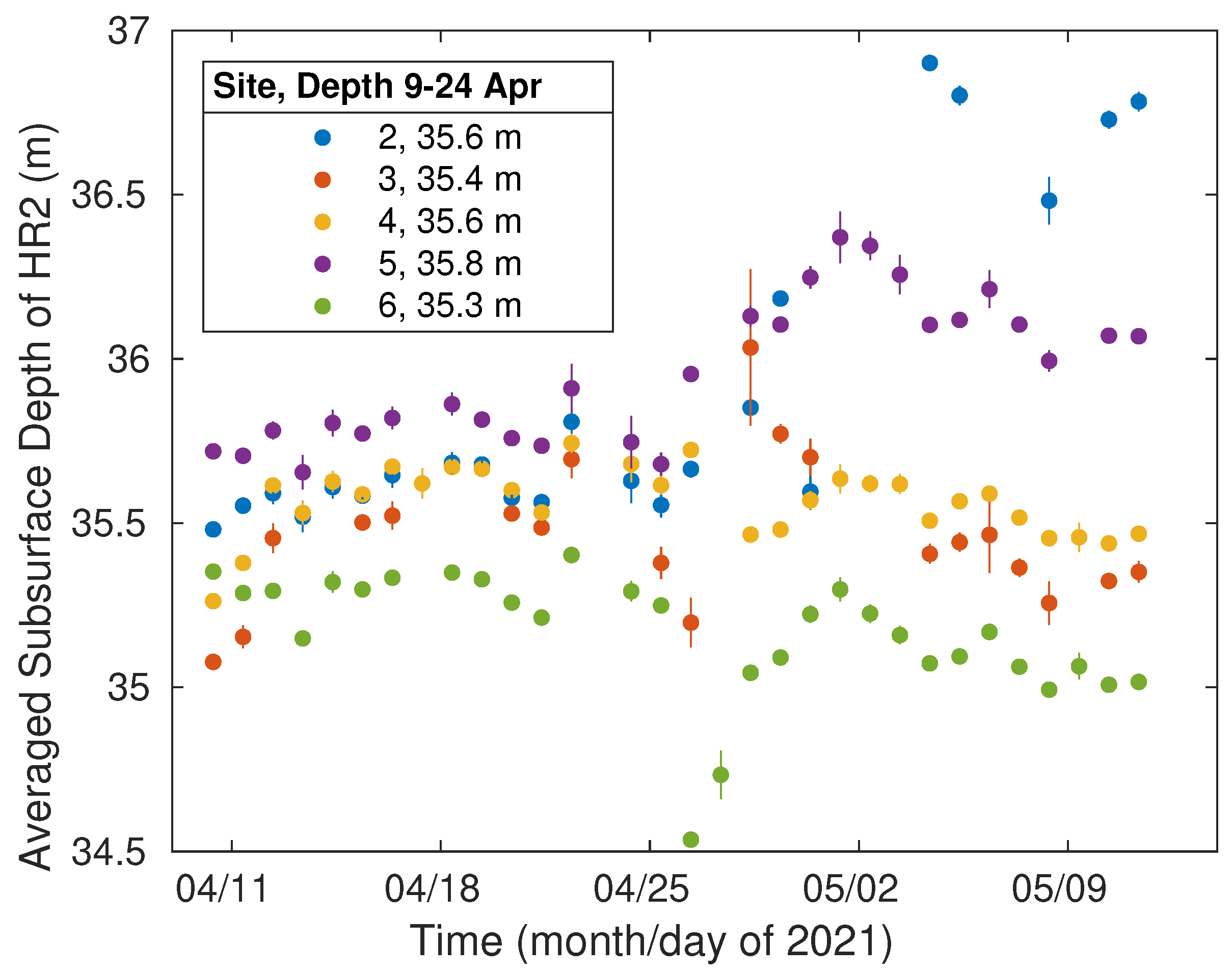
Figure 4.
Separations between stations. Left insets show separation changing by about 1 m over the semidiurnal tidal time scale. The lower left inset also plots normalized tidal current (gray). Right inset shows depth at site 5 and also distance to a nearby reflective object.
Figure 4.
Separations between stations. Left insets show separation changing by about 1 m over the semidiurnal tidal time scale. The lower left inset also plots normalized tidal current (gray). Right inset shows depth at site 5 and also distance to a nearby reflective object.
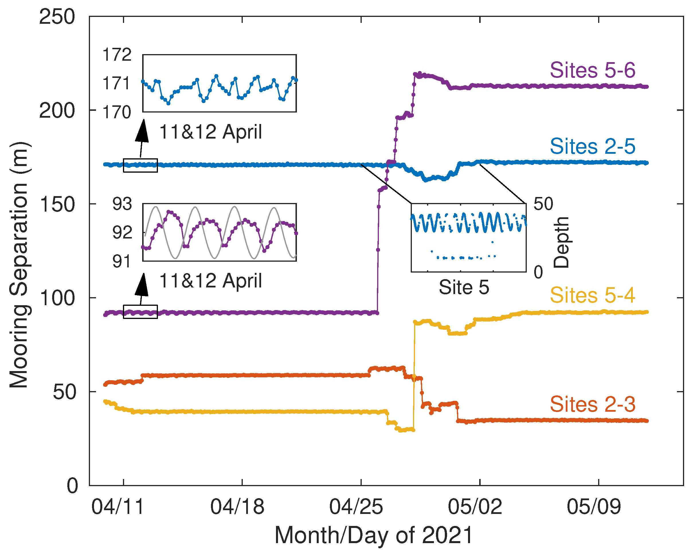
Figure 5.
Tilt measured by the HR2 at site 6 (top) and current along drifter tracks that passed over the volcanic plateau (bottom).
Figure 5.
Tilt measured by the HR2 at site 6 (top) and current along drifter tracks that passed over the volcanic plateau (bottom).
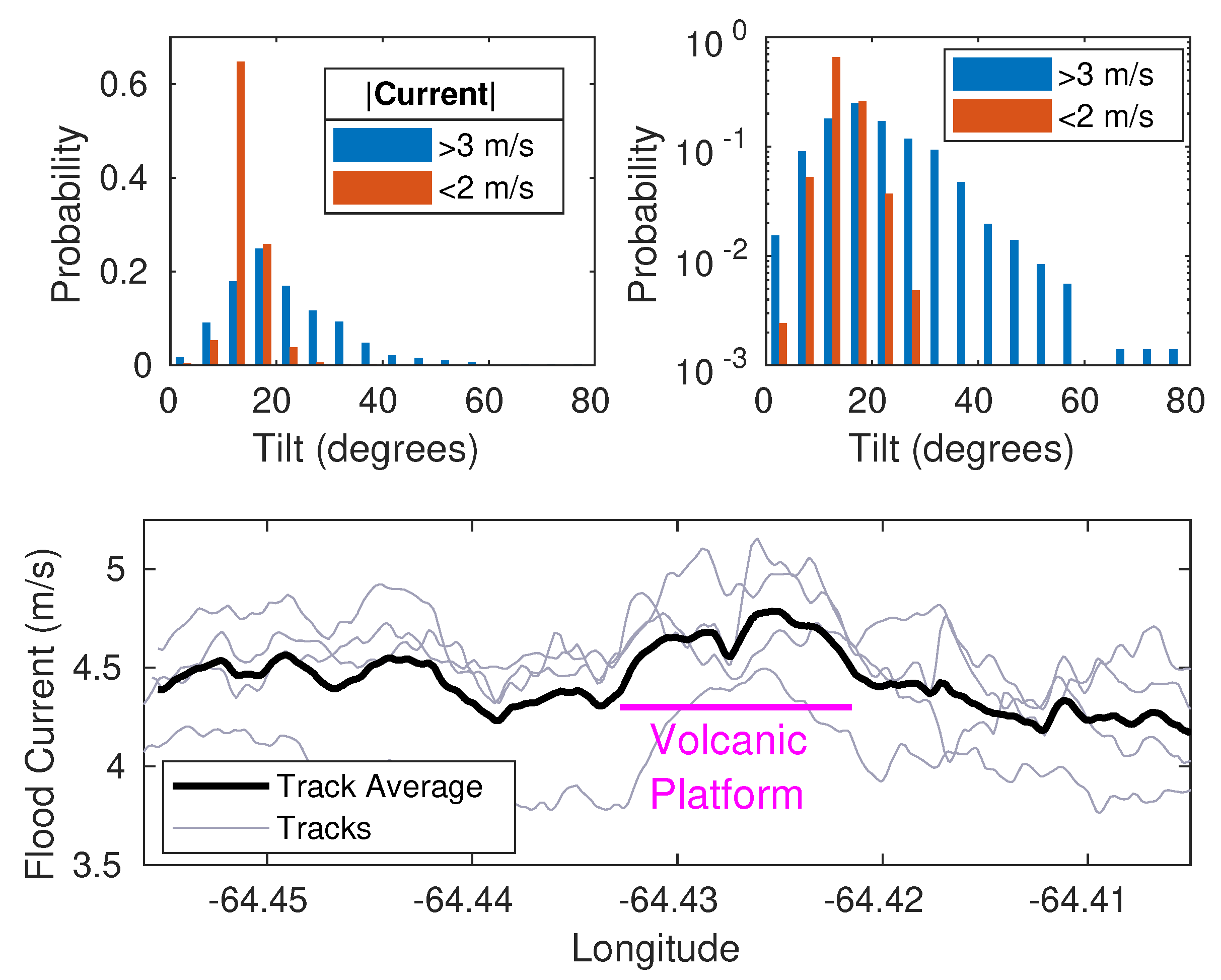
Figure 6.
Comparison of detection efficiency for signal propagation from site 1 to 4 (193 m range) and from site 7 to 4 (202 m range).
Figure 6.
Comparison of detection efficiency for signal propagation from site 1 to 4 (193 m range) and from site 7 to 4 (202 m range).
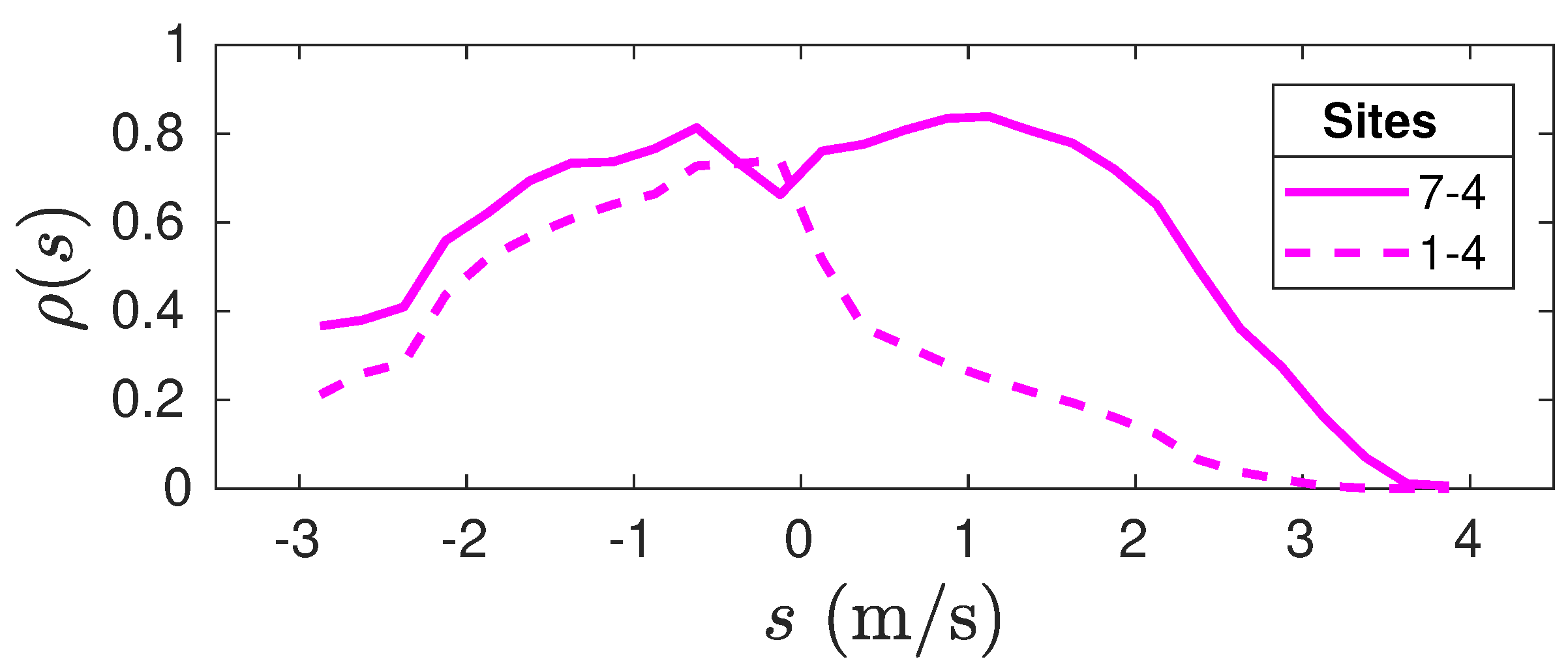
Figure 7.
Detection efficiency as a function of current speed (positive flood, negative ebb) and range for HR signals transmitted by the tags and detected by HR2 units. Measurements were obtained at ranges between sites indicated by labelling beside magenta line-ticks.
Figure 7.
Detection efficiency as a function of current speed (positive flood, negative ebb) and range for HR signals transmitted by the tags and detected by HR2 units. Measurements were obtained at ranges between sites indicated by labelling beside magenta line-ticks.
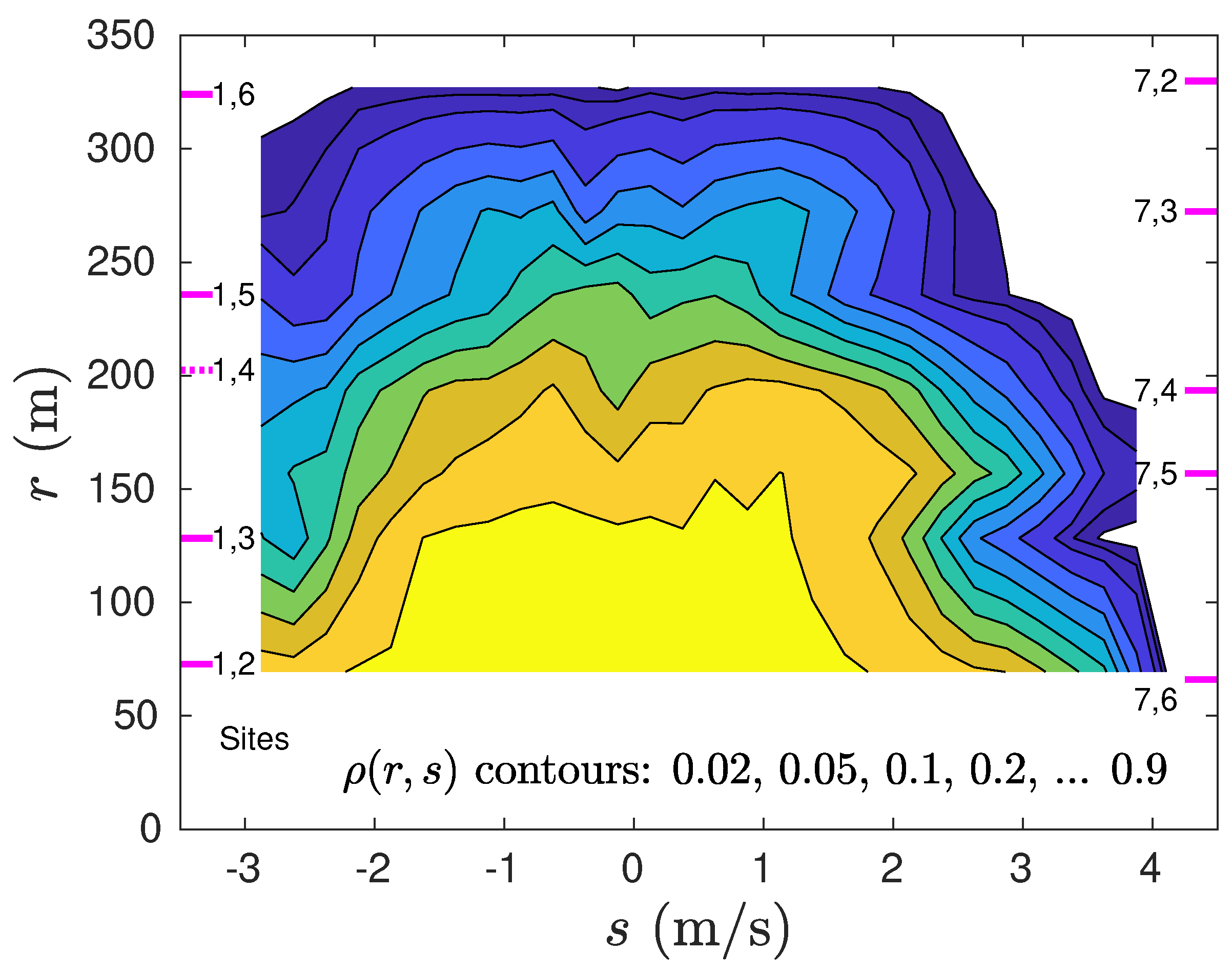
Figure 8.
Probability that HR transmissions between sites 4 and 5 will be detected during each 10 minute interval (blue). Green shading shows flood tide normalized by 5 ms. Red shows range between the sites.
Figure 8.
Probability that HR transmissions between sites 4 and 5 will be detected during each 10 minute interval (blue). Green shading shows flood tide normalized by 5 ms. Red shows range between the sites.
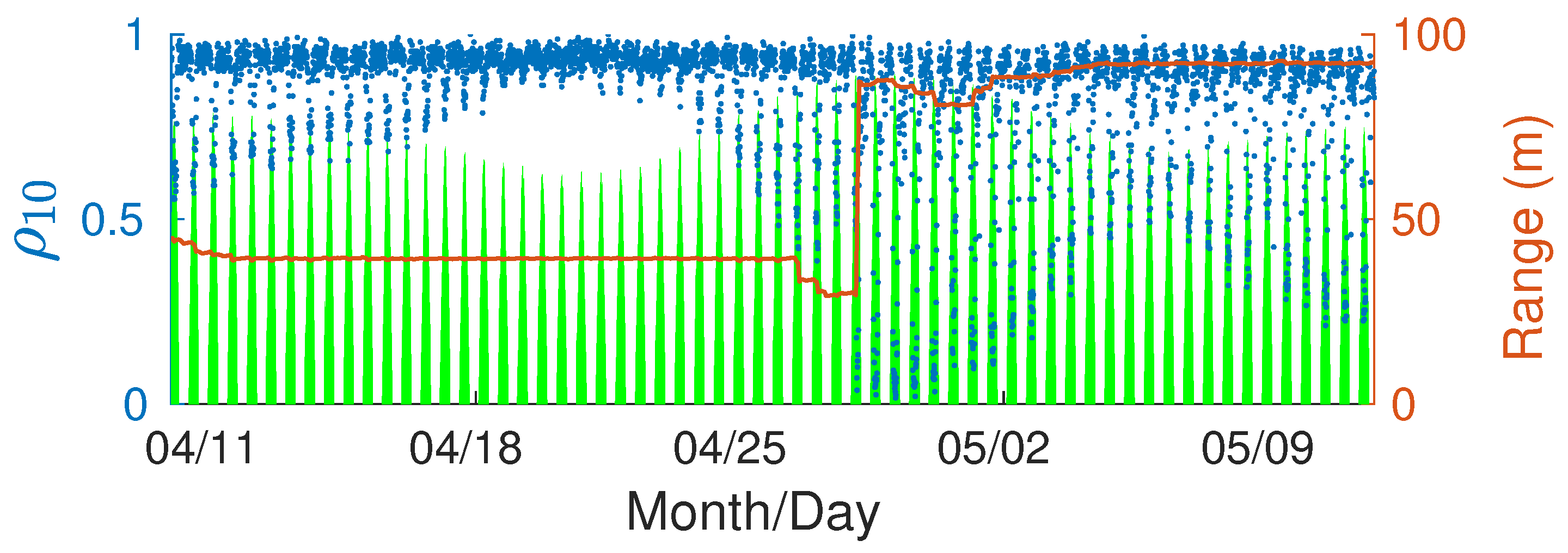
Figure 9.
Detection efficiency, HR signals transmitted by one HR2 and detected by another HR2. Ranges measured are indicated in magenta and sites associated with each range are labeled to the right.
Figure 9.
Detection efficiency, HR signals transmitted by one HR2 and detected by another HR2. Ranges measured are indicated in magenta and sites associated with each range are labeled to the right.
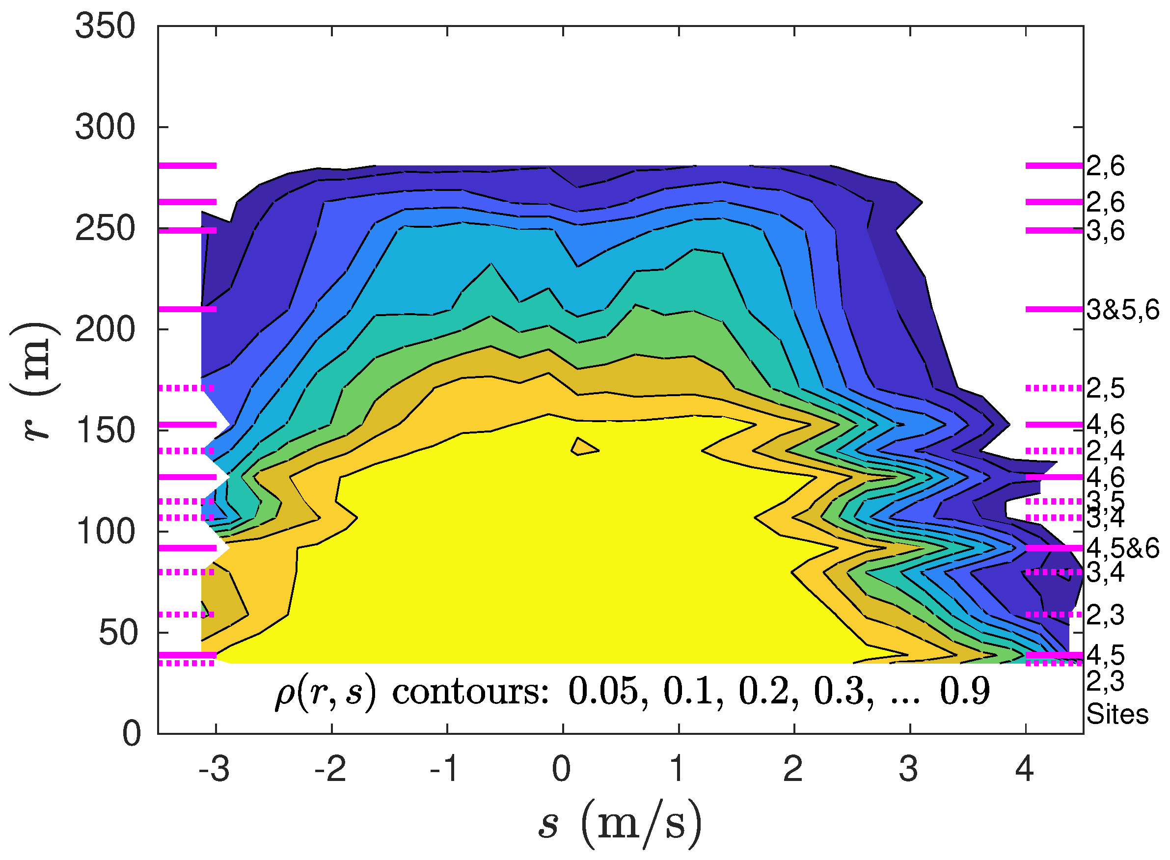
Figure 10.
Distribution of current when sampled uniformly (blue), sampled when the HR signal was detected at 1.25 m range (green), and sampled when HR was detected at more distant sites (orange). Wiskers on the probability density function indicate ± two standard errors.
Figure 10.
Distribution of current when sampled uniformly (blue), sampled when the HR signal was detected at 1.25 m range (green), and sampled when HR was detected at more distant sites (orange). Wiskers on the probability density function indicate ± two standard errors.
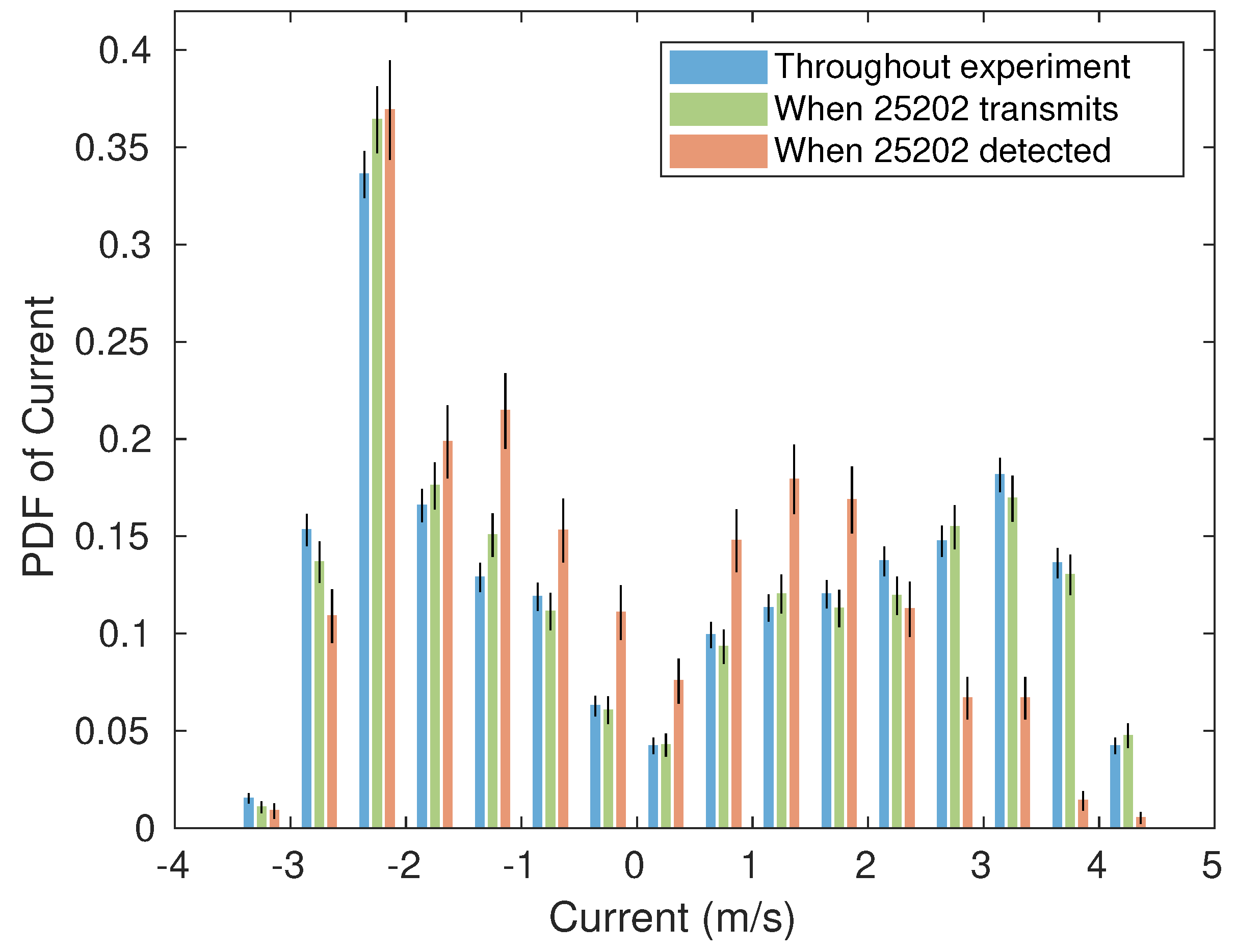
Figure 11.
Detection efficiency underestimates the probability of a detection-positive 120 s interval.
Figure 11.
Detection efficiency underestimates the probability of a detection-positive 120 s interval.
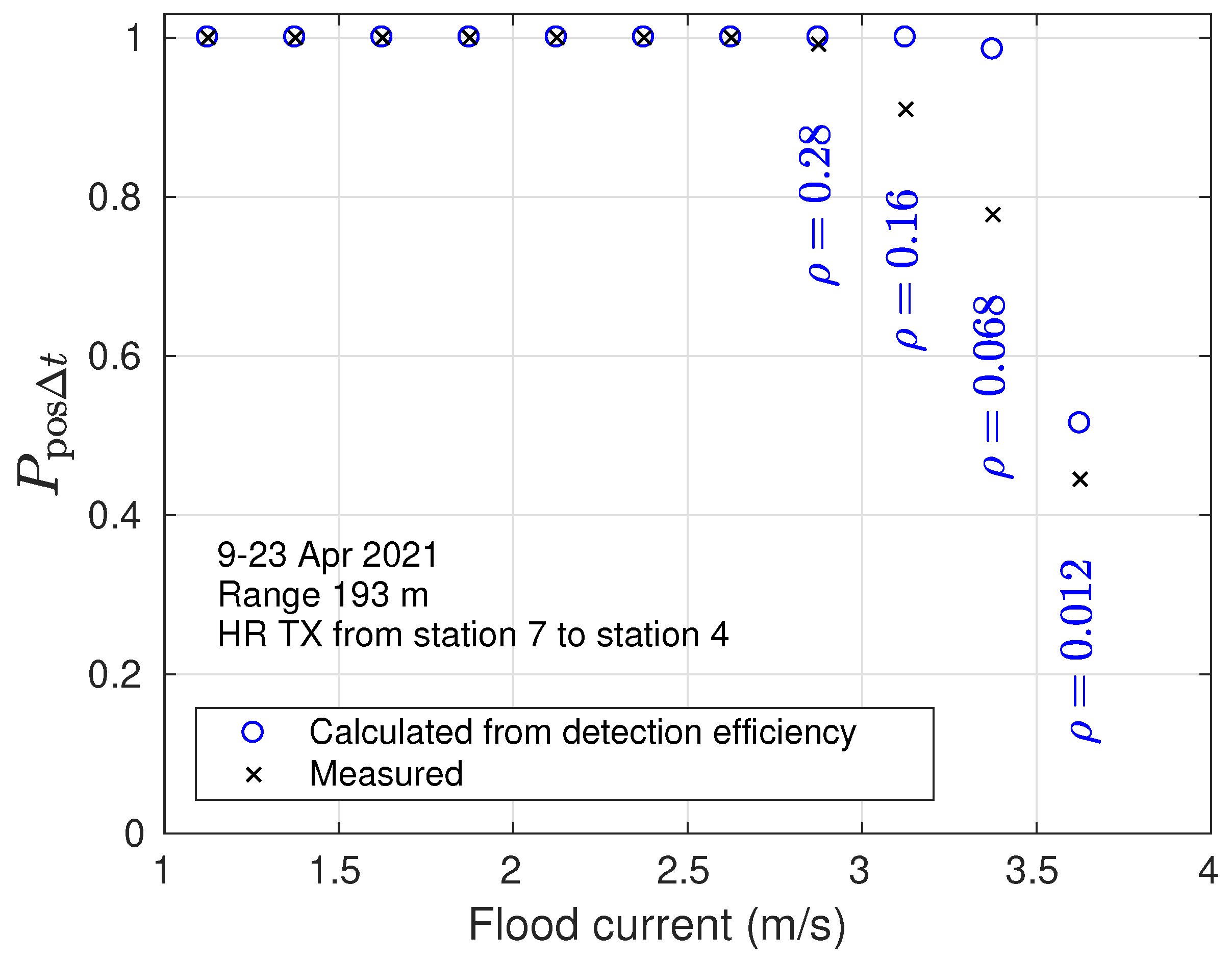
Figure 12.
Finalized detection efficiency is obtained by selecting those HR2-HR2 propagation paths that do not appear to be blocked by variations in seafloor topography. It is also considered that all HR signals would be detected at near-zero range, regardless of current speed. Tag-HR2 transmissions were used to add probabilities at the greatest range (green line, top-right corner).
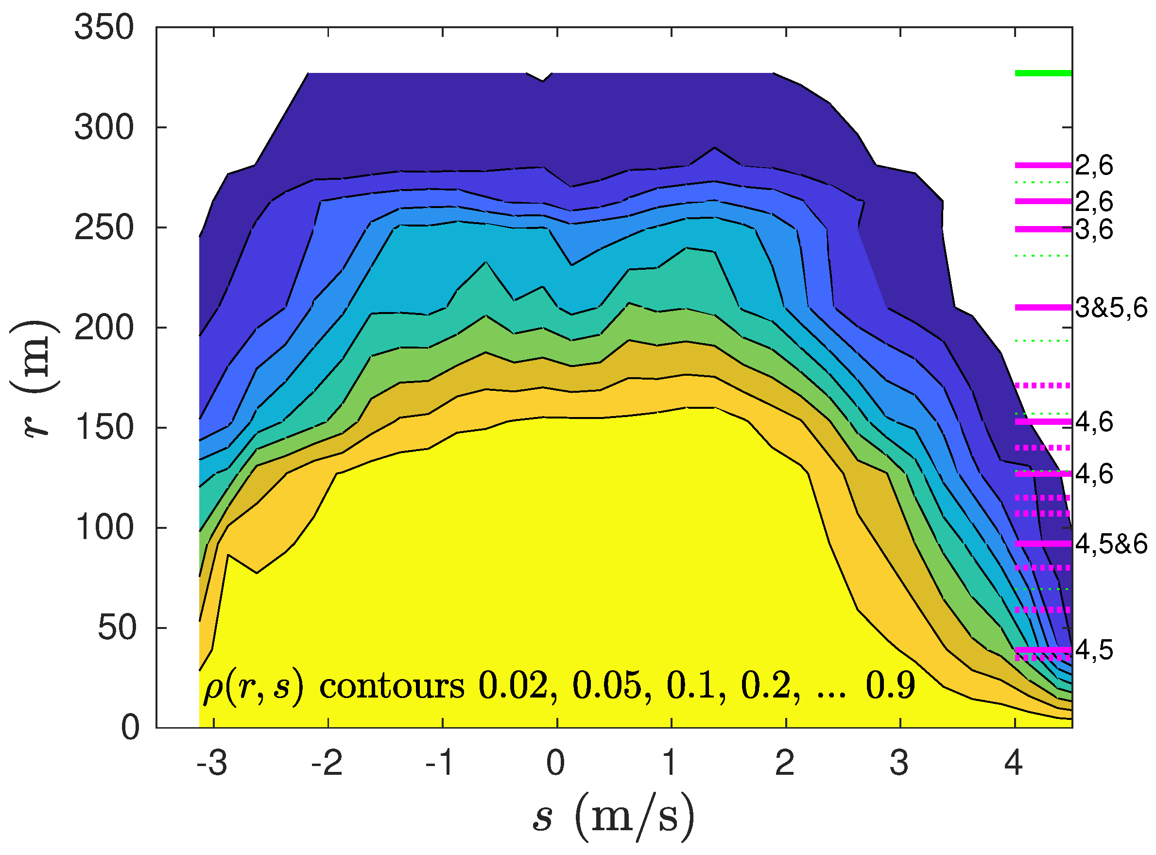
Figure 13.
Effective detection range obtained by integrating the probability that an HR signal is detected. Using HR2-to-HR2 transmission paths that do not exhibit obvious blocking (blue), all of the HR2-to-HR2 transmission paths that were measured (red), and tag-HR2 transmission paths (orange).
Figure 13.
Effective detection range obtained by integrating the probability that an HR signal is detected. Using HR2-to-HR2 transmission paths that do not exhibit obvious blocking (blue), all of the HR2-to-HR2 transmission paths that were measured (red), and tag-HR2 transmission paths (orange).
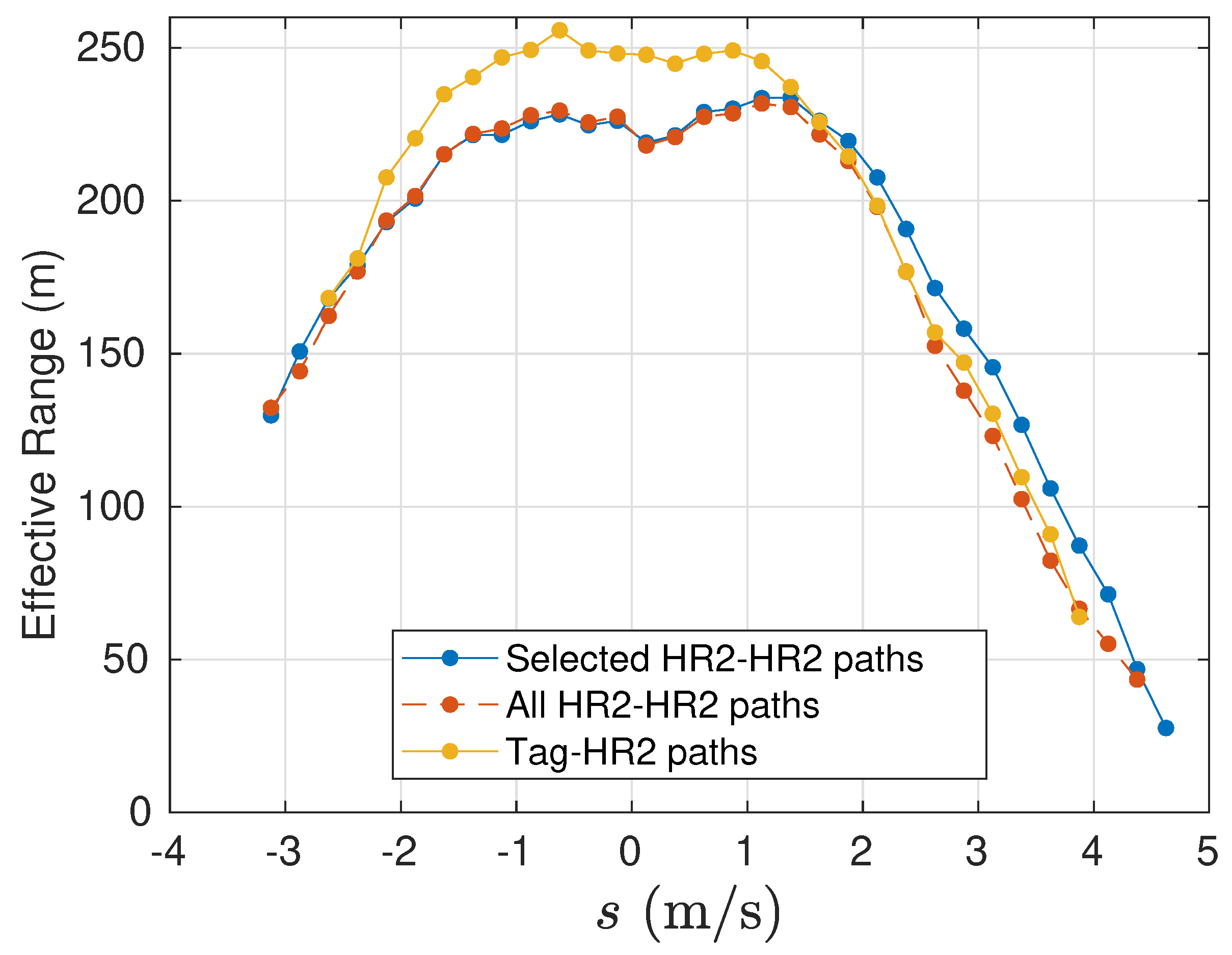
Figure 14.
Ratio of detection efficiency of HR tag signals relative to detection efficiency of PPM tag signals. Contours are on a geometric scale.
Figure 14.
Ratio of detection efficiency of HR tag signals relative to detection efficiency of PPM tag signals. Contours are on a geometric scale.
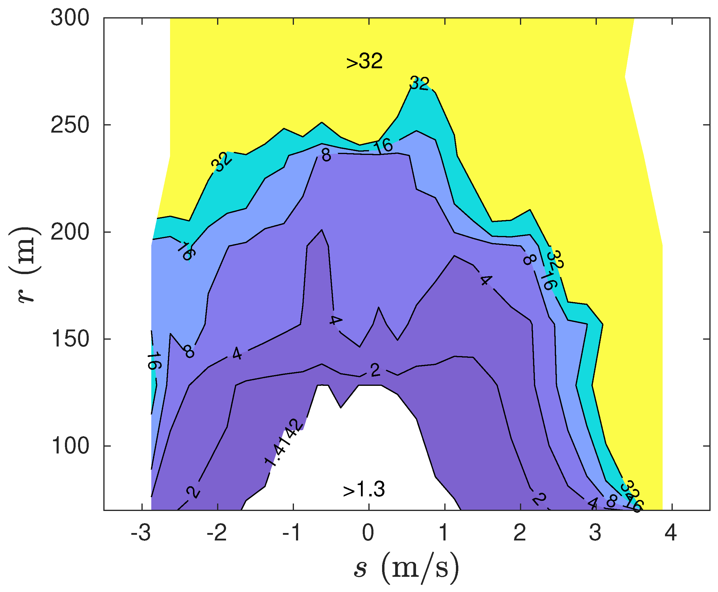

Table 1.
Mooring locations and depths at low tide.
| Site | Latitude | Longitude | Depth (m) | Device | HR TX-interval (s) |
|---|---|---|---|---|---|
| 1 | 45.3623 | -64.4316 | 34 | Tag | 1.8-2.2 |
| 2 | 45.3628 | -64.4314 | 33 | HR2 | 4-6 |
| 3 | 45.3634 | -64.4310 | 32 | HR2 | 25-35 |
| 4 | 45.3640 | -64.4308 | 34 | HR2 | 4-6 |
| 5 | 45.3644 | -64.4304 | 34 | HR2 | 4-6 |
| 6 | 45.3650 | -64.4300 | 34 | HR2 | 4-6 |
| 7 | 45.3656 | -64.4296 | 33 | Tag | 1.8-2.2 |
Table 2.
The number of HR signals transmitted X and detected between sites.
| Sites | X | Number removed | Troublesome number | |||
|---|---|---|---|---|---|---|
| 621816 | 537521 | 27686 | 4619 | 0.8644 | 0.0515 | |
| 620704 | 452490 | 30101 | 12349 | 0.7290 | 0.0665 | |
| 1053057 | 932725 | 51033 | 7021 | 0.8857 | 0.0547 | |
| 1055051 | 567080 | 34185 | 33396 | 0.5375 | 0.0603 |
Table 3.
Ranges from tags to HR2 receivers. GPS ranges are from vessel position when the mooring was dropped overboard.
Table 3.
Ranges from tags to HR2 receivers. GPS ranges are from vessel position when the mooring was dropped overboard.
| Tag-HR2 sites | Drop range (m) | range (m) |
|---|---|---|
| 1-2 | 62 | 73 |
| 1-3 | 139 | 128 |
| 1-4 | 202 | 202 |
| 1-5 | 257 | 236 |
| 1-6 | 337 | 324 |
| 7-2 | 345 | 330 |
| 7-3 | 267 | 272 |
| 7-4 | 204 | 193 |
| 7-5 | 149 | 157 |
| 7-6 | 69 | 66 |
Table 4.
Ranges used to calculate detection efficiency.
| n | Separation (m) | Mooring Sites | Transmission Characteristic |
|---|---|---|---|
| 1 | 2,3 | blocking | |
| 2 | 4,5 | no blocking | |
| 3 | 2,3 | blocking apparent | |
| 4 | 3,4 | blocking apparent | |
| 5 | 4,5 & 5,6 | no blocking | |
| 6 | 3,5 | blocking | |
| 7 | 3,5 | blocking | |
| 8 | 4,5 | no blocking | |
| 9 | 2,4 | blocking | |
| 10 | 4,6 | no blocking | |
| 11 | 2,5 | blocking | |
| 12 | 3,6 & 5,6 | no blocking | |
| 13 | 3,6 | no blocking | |
| 14 | 2,6 & a few at 3,6 | no blocking | |
| 14 | 2,6 | no blocking |
Disclaimer/Publisher’s Note: The statements, opinions and data contained in all publications are solely those of the individual author(s) and contributor(s) and not of MDPI and/or the editor(s). MDPI and/or the editor(s) disclaim responsibility for any injury to people or property resulting from any ideas, methods, instructions or products referred to in the content. |
© 2023 by the authors. Licensee MDPI, Basel, Switzerland. This article is an open access article distributed under the terms and conditions of the Creative Commons Attribution (CC BY) license (http://creativecommons.org/licenses/by/4.0/).
Copyright: This open access article is published under a Creative Commons CC BY 4.0 license, which permit the free download, distribution, and reuse, provided that the author and preprint are cited in any reuse.


