
Submitted:
13 October 2024
Posted:
15 October 2024
You are already at the latest version
Abstract
The communication space allows for the exchange of information and ensures the movement of material flows and passenger flows. By communication space, we mean the movement of information and material flows of various natures based on transport systems, in this case, air transport systems. The direction and intensity of these flows to varying degrees reflect the main social and economic processes. Time series reflecting the intensity of passenger flows and cargo transportation over a given time horizon were selected as a source of information used for analysis. An information-theoretical measure based on the assessment of entropy transfer between time series elements is used as a research tool. Based on the obtained paired estimates of entropy transfer between the selected time series, an entropy transfer matrix is formed, which allows considering a set of time series as a communication system within the framework of system analysis. The resulting matrices are used to form entropy transfer graphs, which allow investigating the properties of time series based on directed graph analysis methods. The article examines examples of the analysis of the cognitive model of transportation, the analysis of the regional communication space, and the analysis of changes in the global communication field.
Keywords:
air transportation
; passengers flows
; cargo flows
; communication space
; time series
; transfer entropy
; entropy transfer graph
; analytics and cognitive computing
1. Introduction
Communication is one of the driving factors of development of human society [1]. Communication, according to Luhmann’s theory, is a key type of operation of social systems; it constitutes systems and ensures their differentiation and reproduction. Social systems and society are communications; systems consist of interconnected communications; society is a special form of social system, including all possible communications [2]. Everything that is not communication is excluded from the operational area of social systems; if there is communication, there is society. If it is possible to identify the signs of communication, then we can talk about the existence of society. If there are no communications in the system, then it is impossible to talk about the existence of a social system. The communication space is a set of communication links of various natures that are generated and perceived by communication agents. Communication agents are understood as separate individuals, groups of individuals, as well as cultural, social, or political institutions. It should be taken into account that each society under consideration forms a unique communication space with its own characteristics and features [3].
In the 21st century, the world communication space is usually associated with the media, the Internet, and the virtual information field [4,5]. However, we should not forget about the real communication processes associated with the movement of a large number of people, including in a short time. These processes are provided exclusively by means of transport systems. For the socio-cultural space, it is not so much the geographical location of the centers of social and cultural attraction that plays an important role, but their transport accessibility. This allows for the formation of a much more complex system of interconnected peripheral and central nodes. On the one hand, transport systems and transport processes are an effective tool for the dense internal aggregation of different spatial segments within the world as a whole. On the other hand, transport facilitates the expansion of individual civilizations into the outside world [6,7]. In this case, not only the ability to get to a certain point in space in a certain time is important, but also the dependence of the economic and cultural components of a given geographic point on transport communications. Despite the fact that individual regions of the world are developing in different directions, the general trend in the development of global society is interconnectedness. This point of view is reflected in one of the modern concepts of world development, namely, connectography. This social hypothesis reflects a new developing trend, which is characterized by active human mobility both from the position of tourism and from the position of migration. Also, within the framework of this hypothesis, an active global exchange of material and intellectual resources is implied. Connectography substantiates the transition from traditional political geography to functional geography. In other words, within the framework of this concept, the emphasis shifts from the official division of the world into countries and regions towards the infrastructure that ensures global socio-cultural and economic ties [8].
Globalization and high technologies contribute to a radical change in the modern socio-cultural and economic space, as well as the system of relationships in it. Transport communications have always played a key role in intercultural exchange between regions, both within individual countries and for the world as a whole. The peculiarities of the formation of transport communications are associated with differences in the economic and geographical position of regions of the world and individual states [9].
A region of the world is determined by the unity of the social, economic, political, and cultural spaces of the countries included in it. The spatial and communication factor is taken into account when studying the history and prospects for the development of society, allowing us to identify key points and time periods based on observed population movements.
Transport systems, regardless of their nature, be it land, air, or water transport, initially have a communication nature. At the present stage, transport is associated primarily with tourism, urbanization, population migration, and globalization [10]. When moving to a new stage of development, regions strive for planned and long-term development of transport infrastructure [11]. In this case, one should focus on global trends in socio-economic development.
Modern air transport is undoubtedly one of the most reliable, high-tech, and high-speed. Air transport occupies a leading position in regional and global passenger transportation, and transports a significant portion of important cargo [12]. Unlike automobile or rail transport, the air transport system allows for the reconstruction of existing routes and the creation of new ones quite easily. The total length of the network of the world air routes is approaching ten million kilometers (Figure 1, [13]). The number of airports in the world is constantly changing due to the construction of new ones and the closure of old airports. However, according to the Federal Aviation Administration (FAA), there are currently about 19,000 airports in the world [14]. The emergence and development of aviation have significantly changed society, both regionally and globally. Air transport has accelerated the processes of socio-cultural interaction and influenced the increase in the number and diversity of communication processes. This has affected people’s daily lives. An example is the express delivery of mail and goods. The cultural aspect is affected by the opportunity to attend theatres, concerts, exhibitions, and sporting events in other cities and sometimes in other countries.
Qualitative leaps in the development of air transport were associated with the development of new types of jet aircraft, including wide-body aircraft. New technologies used in the creation of aircraft and their components and units, including jet engines, have made it possible to significantly improve the performance characteristics of aircraft and, consequently, reduce the life cycle costs of aircraft and aircraft engines [15,16]. This made it possible to increase the efficiency of transportation by increasing the size and range of airliners, reduce ticket prices, and increase the intensity of economic and socio-cultural exchange between Asia and the rest of the world in the late 1980s and in 2010 [9].
Other important factors changing the air transport landscape include the emergence of low-cost carriers (LCCs), the deregulation of air travel since the late 1970s, and the liberalization of emerging air travel markets such as China, Indonesia, India, and Brazil [17]. Open skies agreements have played an important role in the development of air transport. Thanks to the signing and implementation of such agreements, the number of restrictions on the nomenclature of carriers and possible routes within the airspace specified in the agreement between the countries has been sharply reduced. The liberalization of air travel in general (a process that includes deregulation and privatization) has led to the growth and diversity of air transport links and increased the adaptability of the global air transport network [18].
In our study, air transport is considered a complex organizational and technical system interacting with various other complex economic and social systems [18]. When defining a system as an object of study, particular attention is paid to the interconnectedness of the system elements [19]. The formed relationships determine the behavior of the system as a whole. In this case, it is not always possible to explicitly determine the influence of some subsystems on others [20].
In our case, to solve the problem, we consider constructing a model of a communication system based on information about passenger and freight flows, since in general they reflect the dynamics of social and economic processes in modern society.
Currently, various methods and algorithms for analyzing time series have been developed that allow constructing various models based on collected statistical data [21,22].
A system model constructed on the basis of time series can be described as a system of differential equations, graphs, and other tools. In this study, we selected the apparatus of discrete mathematics—graphs, which are a popular and effective tool for analyzing complex systems reflecting the behavior of the communication space [23,24].
When analyzing complex systems, an analysis method is used based on the decomposition of the system into subsystems and the construction of hierarchical relationships between them [25,26]. Depending on the level of the hierarchical subsystem: the executive level, the coordination level, and the planning level, it is necessary to build models that reflect the properties of each of these levels. When considering the air transport system, one can identify a hierarchy of problem solving for analyzing communication at the regional level, the level between regions, and the global level of interregional transportation.
2. Methods of Analysis
Statistical data reflecting the quantitative characteristics of passenger and cargo flows at selected time intervals are used as a source of analysis of the communication space. The data is obtained from open sources (reports and databases) and is presented in the form of time series.
When formalizing the problem statement, mathematical objects are used: time series, matrices, the concept of entropy, entropy transfer, graphs, entropy transfer graphs. Next, we will consider the elements of the analysis used to construct entropy transfer graphs, on the basis of which we can draw a conclusion about the properties of the communication space under consideration.
2.1. Problem Formulation
We consider a system Ks, based on a set of time series S:
where n is the number of time series used in the analysis of the system Ks.
S = [s1, s2, …, sn ],
It is necessary to construct a model of the communication system Ks, using time series set and presented as a transfer entropy graph.
2.2. Procedure for Constructing an Entropy Transfer Graph
When analyzed the influence of one process over time on another process, a measure of influence called transfer entropy (TE) is used [27]. This measure refers to theoretical-information characteristics and is based on Shannon’s information entropy.
To analyze the system of time series Ks, we need to construct a mapping (algorithm) that would allow us to move from a set of time series to a matrix whose elements would reflect the mutual influence of selected pairs of time series over a given time interval.
Thus, we need to determine a set of pairs of numbers over a certain time interval, which allows us, on the one hand, to evaluate the influence of time series in the context of their direction of influence on each other and, on the other hand, to obtain a pair of quantitative characteristics when constructing an information transfer matrix.
The matrix elements reflect the systemic connections in a set of time series.
When constructing a matrix whose elements are pairs of numbers, we fold the Ks system into a real matrix Ms.
Then, the matrix Ms now can be associated with the adjacency matrix of the GTE graph.
Applied the matrix Ms, the entropy transfer graph GTE can be constructed. The vertices of this matrix are the names of time series, and the edges determine the presence of a connection between the vertices; the weights of the edges reflect the strength of the influence of one process in time on another process.
The structure of this graph reflects the entropy of the system. The value of entropy of this graph depends on the adopted measure.
In the simplest case, the entropy of a matrix is determined depend on its structural properties. For example it is the power of the set of the weights |V| of matrix MTE, where V is the set of edges of the MTE matrix.
One of the graph analysis algorithms that can be useful in our case is the analysis of the maximum flow on graphs [28].
Maximum flow route can be used in the analysis of the properties of various transport networks. It allows you to estimate the throughput of the selected route on graphs.
2.3. Method of Analyzing the Communication Properties of Air Transportation
Next, the problem of analyzing communications at various levels of territorial organization is considered: regional, federal and world regions. The subject of analysis is data sets presented in the form of time series reflecting the flows of transported passengers and cargo transportation in certain periods of time. The main research tool is an information-theoretical measure based on the assessment of the transfer of entropy between the elements of time series.
It should be noted that if the data are presented in the form of multivariate time series, the analysis is carried out on the basis of paired comparisons at specified time intervals, which allows us to construct a matrix of paired comparisons. This matrix is then used as a conjugacy matrix when constructing an entropy transfer graph.
The resulting matrices for different time intervals are considered as adjacency matrices for entropy transfer graphs, which allow us to study the properties of the system represented by time series based on various graph analysis methods.
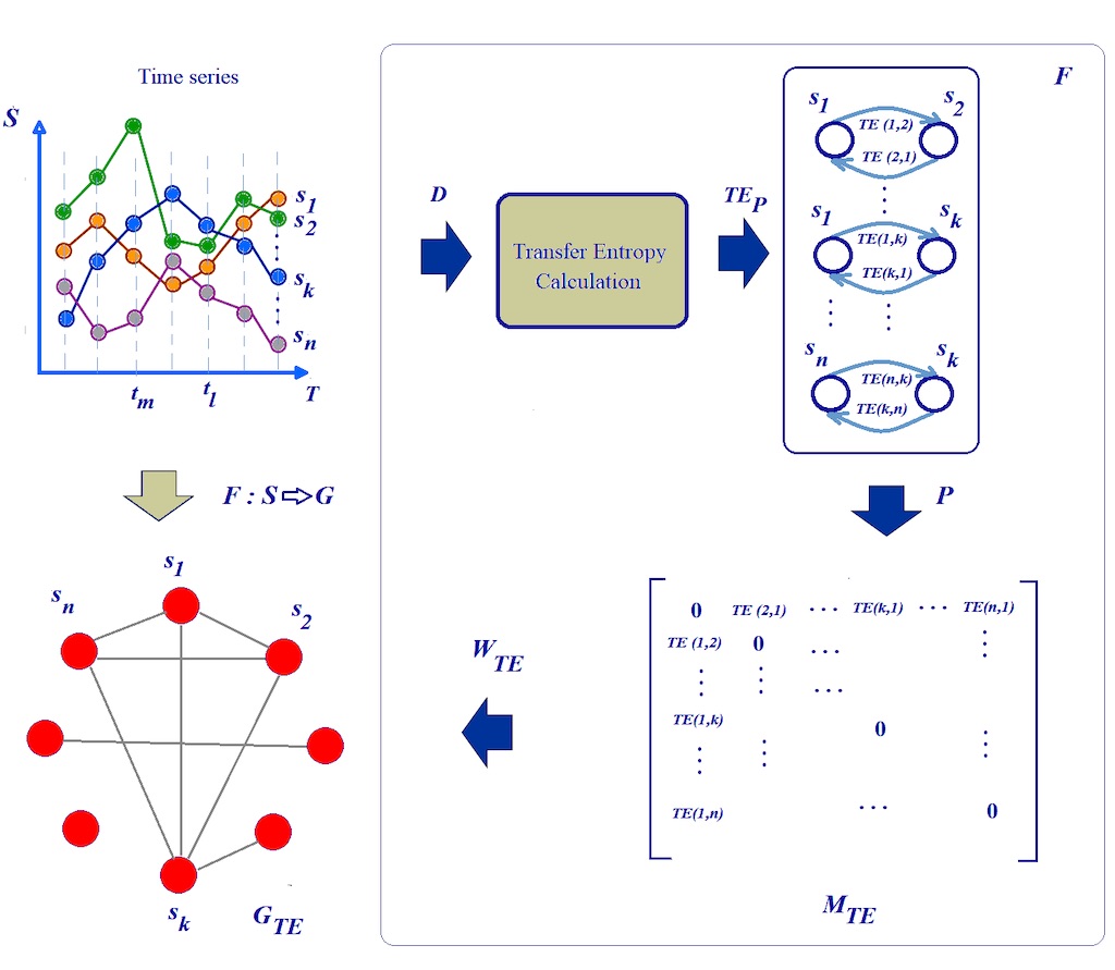
Figure 2 shows the main stages of the formation of the entropy transfer graph GTE based on the time series system Sn, where Sn are time series, D are the values of the time series on the selected time interval tm, P is a set of paired estimates pmi,j, MTE is a matrix composed of the values of paired estimates of the transfer of entropy, GTE is a graph (model) of the system of communication interactions of processes, F is a mapping of S into graph G.
3. Case Studies
In Section 3.1 we will consider the analysis of the communication space for passenger transportation in the system of one region. In Section 3.2 we will consider the problem of analyzing the communication space using the example of interregional transportation and the center. In Section 3.3 we will consider the problem of analyzing changes in the properties of the communication space over a long time horizon using the example of regional world passenger transportation.
3.1. Regional Transportation
The airport network reflects the economic and social characteristics of the region and is an integral part of the transport system for the carriage of passengers and cargo by air. Airports provide reliable logistics links within the region, countries, and regions of the world. Airport congestion, and thus passenger traffic, reflects the geographical, social, and economic characteristics of the region, directly affecting the characteristics of the communication space. Airport capacity statistics reflect the overall traffic of aircraft, the directions of air transport movement, and the intensity of the flow of passengers and cargo.
Let us further consider the analysis of the activities of the airport network of one region over a certain period of time using the example of Great Britain. Statistical data were collected by the Civil Aviation Authority [29]. The statistics reflect the operating characteristics of more than 60 airports in Great Britain from 1981 to 2015. Figure 3 shows curves reflecting the main characteristics of the intensity of traffic flows: total traffic density, air transport traffic density, and cargo traffic density.
Figure 4 shows the corresponding flow change curve for registered passengers over the same period of time.
Using the previously presented method for analyzing the mutual influence of processes Sn (n=1…4), we determine the values of the set of paired estimates of transfer entropy P and form the MTE matrix. The calculation results are presented in Table 1.
Next, we present the data from Table 1 as a directed graph GTE = (N,V), where N is the set of vertices describing processes in time, V is the set of edges whose weights reflect the information measure of entropy transfer between processes.
Figure 5a shows the GTE graph, where node 1 is Total Movements, node 2 is Air Transportation Movements, node 3 is Terminal Passengers, node 4 is Freight Tonness.
Figure 5b shows the approximation of the GTE graph in the form of a GTES graph, in which edges with small weights (c<0.095) are removed. The GTES graph reflects the cause-and-effect relationship between the processes of organizing transportation.
This model in the form of a GTES graph can be used as a knowledge representation model for forming a data structure in a graph database, which can be used to solve various problems of analyzing the activities of the country’s airport network and assessing the performance indicators of the passenger and cargo transportation system, which in turn will allow assessing the properties of the communication space.
3.2. Analysis of the Communication Space of the Center and Regions
The regional transport system is a complex of subsystems interacting with regional systems of air transport, land transport and water transport. The organization of these systems has a hierarchical structure, requiring the solution of problems of coordination and synchronization of transportation participants [11].
A large role in the airport system is given to aviation hubs, allowing solving problems of synchronization and coordination in transportation system.
Let us consider an example how we can analyze the communication space of the center and regions.
The airports of Moscow were chosen as air hubs: Vnukovo Airport, Domodedovo Airport and Sheremetyevo Airport. The airports of Ufa city, Yekaterinburg city and Chelyabinsk city were chosen as regional airports. These airports are used for the transportation of goods and passengers, including the movement of labor capital, tourist flows, influencing the social landscape of the regions. They are usually having deep connection connected with large aviation hubs.
The analysis of the communication space is carried out on the basis of statistics of passenger and cargo flows for all selected airports (from 01.01.2018 to 31.08.2018). The statistical data are presented in the form of graphs in Figure 6 and Figure 7 [30]
Next, based on the available statistical information, we will construct the MTE matrix for the GTE graph, the weight values of which are presented in Table 2. The GTE vertices are numbered in accordance with the row numbers in Table 2, i.e., 1 – Yekaterinburg, 2 – Chelyabinsk, 3 – Ufa, 4 – Moscow (Vnukovo), 5 -Moscow (Domodedovo), 6 – Moscow (Sheremetyevo).
An illustration of the obtained results in the form of a graph model is presented in Figure 8. From the analysis of the communication space based on the obtained results, it follows that there is some heterogeneity in the communication spaces for regional air transport hubs and the center, which requires increasing the efficiency of solving the problems of managing the coordination of regions and the center.
3.3. Air Transportation between World Regions and Communication Space
When analyzing time series that describe processes in a system, in our case, a communication space based on air transportation, the task of analyzing a set of regional subsystems as a single whole arises, which would reflect the properties of the global communication space
In this example, an analysis of passenger transport flows between different regions of the world is performed, which allows us to evaluate the dynamic properties of the world communication space. The following statistical regions of the world according to ICAO were selected: Africa Eastern and Southern, Africa Western and Central, Arab World, Central Europe and the Baltics, East Asia & Pacific, Europe & Central Asia, European Union, Latin America & Caribbean, Middle East & North Africa, North America, South Asia, Sub-Saharan Africa [31]. The integrating indicator is the total registered indicator of passenger transportation volume: World. Figure 9 shows the geography of these regions.
Figure 10 shows curves describing the change in the flow of air passenger traffic in regions and between regions of the world for the period 1970-2021. The data was divided into decades, which allows us to assess the changes in the influence of regions on communication directions over these years.
Table 3, Table 4, Table 5, Table 6, Table 7, Table 8 and Table 9 show the results of calculating transfer entropy by decades.
Sets of GTE graphs obtained on the basis of the analysis of transfer entropy for different time periods presented in Table 3, Table 4, Table 5, Table 6, Table 7, Table 8 and Table 9 are shown in Figure 11, Figure 12, Figure 13, Figure 14, Figure 15, Figure 16 and Figure 17.
Let us further consider the results of the analysis of changes in the directions of air passenger flows over time, as an illustration of the dynamics of the communication space.
Analysis of changes in the communication space based on air transport between regions of the world shows dynamic features of changes in the properties of this space, which corresponds to the concepts of nonequilibrium complex dynamic systems, or the process of self-organization. Communication flows change dynamically depending on economic, political, social and technological factors. Analysis of the communication space allows us to assess the state of the world system from the standpoint of its sustainable development.
3.4. TE Graph Max Flows Analysis
Next, we will consider an example of constructing maximum entropy transfer flows based on the algorithm for determining the maximum flow in the graph [28].
As an example, we will consider the period from 2001 to 2010 (Figure 18).
Figure 19a–d shows the results of calculating the maximum flows between the selected nodes of the GTE graph (2001-2010). When designating the graph vertices, the abbreviations of statistical regions according to the ICAO version were used.
The presented results of the analysis can be useful in assessing the development of the communication field between regions over a given period of time.
For following statistical regions of the world according to ICAO [31] that were selected the following abbreviations were applied in Figure 19: AE&S - Africa Eastern and Southern, AW&C - Africa Western and Central, AW- Arab World, CE&B - Central Europe and the Baltics, EA&P - East Asia & Pacific, E&CA - Europe & Central Asia, EU - European Union, LA&C - Latin America & Caribbean, ME&NA - Middle East & North Africa, NA -North America, SA - South Asia, SSA - Sub-Saharan Africa, W - World.
So, we can conclude that the results of analysis obtained showed that transfer entropy flows between world regions change dynamically depending on political, economic, social and technological factors that manifest themselves over a historical period of time.
4. Conclusions
The basis for sustainable development of modern society is the communication space. The article considers the problem of analyzing the communication space at various levels of its organization of regions, federation and regions of the world based on air transportation data.
A method for analyzing communication space is proposed based on the construction of a graph model of entropy transfer, which is based on time series and an entropy transfer algorithm.
The object of analysis is a set of time series reflecting the flows of transported passengers and cargo, and the tool is the transfer of entropy between time series.
The results obtained showed that transfer entropy flows change dynamically depending on political, economic, social and technological factors that manifest themselves over a historical period of time.
The analysis of cargo flows and passenger flows is carried out using the example of a region, regions and the center, regions of the world.
Based on the analysis of the activities of the airport network of a region, a graph model is built, which can be used as a model of the data structure in a graph database to solve various problems of assessing the performance indicators of the regional airport network and the system of passenger and cargo transportation, thereby allowing to assess the structure of the communication space.
An example of applying the theoretical-information approach to the analysis of air transportation between regions and hubs of the center in order to study the features of communication spaces is considered.
An analysis of the communication space based on air transportation between regions of the world was conducted, which revealed dynamic features of changes in the properties of the communication space. This is consistent with the behavior of complex dynamic systems and corresponds to the processes of self-organization in these systems.
In general, the analysis of the communication space allows us to assess the state of society from the standpoint of sustainable development.
Author Contributions
Conceptualization, S.V.; methodology, S.V. and N.K.; investigation, N.K.; writing—original draft preparation, N.K.; writing—review and editing, S.V.; supervision, S.V. All authors have read and agreed to the published version of the manuscript.
Funding
This research received no external funding.
Institutional Review Board Statement
Not applicable.
Informed Consent Statement
Not applicable.
Data Availability Statement
Data supporting the results presented in this paper are available upon reasonable request.
Conflicts of Interest
The authors declare no conflicts of interest.
References
- Luhmann, N. ; Social Systems; Stanford University Press: Stanford, UK, 1995. [Google Scholar]
- Borch, C. ; Niklas Luhmann: In Defence of Modernity; Routledge: Milton Park, UK, 2011. [Google Scholar]
- Castells, M. ; The Information age: Economy, Society and Culture; Wiley-Blackwell: Malden, USA, 2000. [Google Scholar]
- Fortner, R.S. ; International communication: History, conflict, and control of the global metropolis, 1st ed.; Cengage Learning: Boston, USA, 1992. [Google Scholar]
- Thussu, D.K. ; International Communication: Continuity and Change, 3rd ed., Bloomsbury Academic: London, UK, 2018.
- Stevenson, R. L. Defining International Communication as a Field. Journalism Quarterly 1992, 69, 543–553. [Google Scholar] [CrossRef]
- New Frontiers in International Communication Theory; Editor Semati, M. ; Rowman & Littlefield: Lanham, USA, 2004.
- Khanna. P.; Connectography: Mapping the Future of Global Civilization; Random House: New York, USA, 2016. [Google Scholar]
- Bowen, J. ; Rodrigue J-P. The Geography of Transport Systems, 6th ed.; Routledge: New York, USA. 2024. [Google Scholar]
- Graham, B. ; Geography and Air Transport; Wiley: Hoboken, USA, 1995. [Google Scholar]
- Faizullin, F.S; Valeev, S.S; Kondratyeva, N.V. Analysis of Regional Air Transportation System as Subsystem of Communication Space, In Proceedings of the International Conference Communication Strategies of Information Society (CSIS 2018), 2019, Atlantis Press, pp. 274-278. [Google Scholar] [CrossRef]
- Adey,P. ; Budd L.; Hubbard P. Flying Lessons: Exploring the Social and Cultural Geographies of Global Air Travel, Progress in Human Geography 2007, 31(6), pp. 773-791. [Google Scholar]
- Live Air Traffic. Available online: www.flightradar24.com (02.10.2024).
- Federal aviation administration. Available online: https://www.faa.gov/ (accessed on 02.10.2024).
- Valeev, S.; Kondratyeva, N. Design of Nonlinear Control of Gas Turbine Engine Based on Constant Eigenvectors. Machines 2021, 9, 49. [Google Scholar] [CrossRef]
- Valeev, S.; Kondratyeva, N. Life Test Optimization for Gas Turbine Engine Based on Life Cycle Information Support and Modeling. Energies 2022, 15, 6874. [Google Scholar] [CrossRef]
- Bowen, J. Low-Cost Carriers in Emerging Countries, 1st ed.; Elsevier: Amsterdam, Netherlands, 2019. [Google Scholar]
- O’Connell, J.F.; Williams, G. Air Transport in the 21st Century. Key Strategic Developments; Routledge: Milton Park, UK, 2011. [Google Scholar]
- Valeev, S.S.; Kondratyeva, N.V. Aviation industry stochastic model based on big data concept. Uchenye Zapiski Kazanskogo Universiteta. Seriya Fiziko-Matematicheskie Nauki 2018. 160 (2), 392-398.
- Valeev, S.S; Kondratyeva, N. V, Large scale system management based on Markov decision process and big data concept. In Proceedings Conference of the 2016 IEEE 10th International Conference on Application of Information and Communication Technologies (AICT), Baku, Azerbaijan, 12-14 Oct. 2016, pp. 6-9.
- Wang, Y.; Zhan, J.; Xu, X.; Li, L.; Chen, P.; Hansen, M. Measuring the resilience of an airport network. Chin. J. Aernaut. 2019, 32, 2694–2705. [Google Scholar] [CrossRef]
- Shi, Z.; Zhang, H.; Li, Y.; Zhou, J. Air Traffic Sector Network: Motif Identification and Resilience Evaluation Based on Subgraphs. Sustainability 2023, 15, 13423. [Google Scholar] [CrossRef]
- Cong, W.; Hu, M.; Dong, B.; Wang, Y.; Feng, C. Empirical analysis of airport network and critical airports. Chin. J. Aeronaut. 2016, 29, 512–519. [Google Scholar] [CrossRef]
- Yang, H.; Le, M.; Wang, D. Airline Network Structure: Motifs and Airports’ Role in Cliques. Sustainability 2021, 13, 9573. [Google Scholar] [CrossRef]
- Zanin, M.; Lillo, F. Modelling the air transport with complex networks: A short review. Eur. Phys. J. Spec. Top. 2013, 215, 5–21. [Google Scholar] [CrossRef]
- Kurant, M.; Thiran, P. Extraction and analysis of traffic and topologies of transportation networks. Phys. Rev. E. 2006, 74, 036114. [Google Scholar] [CrossRef] [PubMed]
- Schreiber, T. Measuring Information Transfer. Physical Review Letters 2000, 85, 461–464. [Google Scholar] [CrossRef] [PubMed]
- Cederbaum, I. On the optimal operation of communication nets. Journal of the Franklin Institute 1962, 274, 130–141. [Google Scholar] [CrossRef]
- UK Airport Data. Available online: https://www.caa.co.uk/data-and-analysis/uk-aviation-market/airports/uk-airport-data/ (accessed on 02.10.2024).
- Federal Air Transport Agency. Available online: https://favt.gov.ru/en/ (accessed on 02.10.2024).
- ICAO Statistical regions. Available online: https://unitingaviation.com/amp/news/economic-development/the-air-transport-monthly-monitor-for-february-2021/ (02.10.2024).
- A Network Map of the World’s Air Traffic Connections. Available online: https://www.visualcapitalist.com/air-traffic-network-map/ (accessed on 02.10.2024).
- The World Bank Group. Available online: https://data.worldbank.org/indicator/IS.AIR.PSGR (accessed on 02.10.2024).
Figure 1.
Air Transportation clusters [13].
Figure 1.
Air Transportation clusters [13].
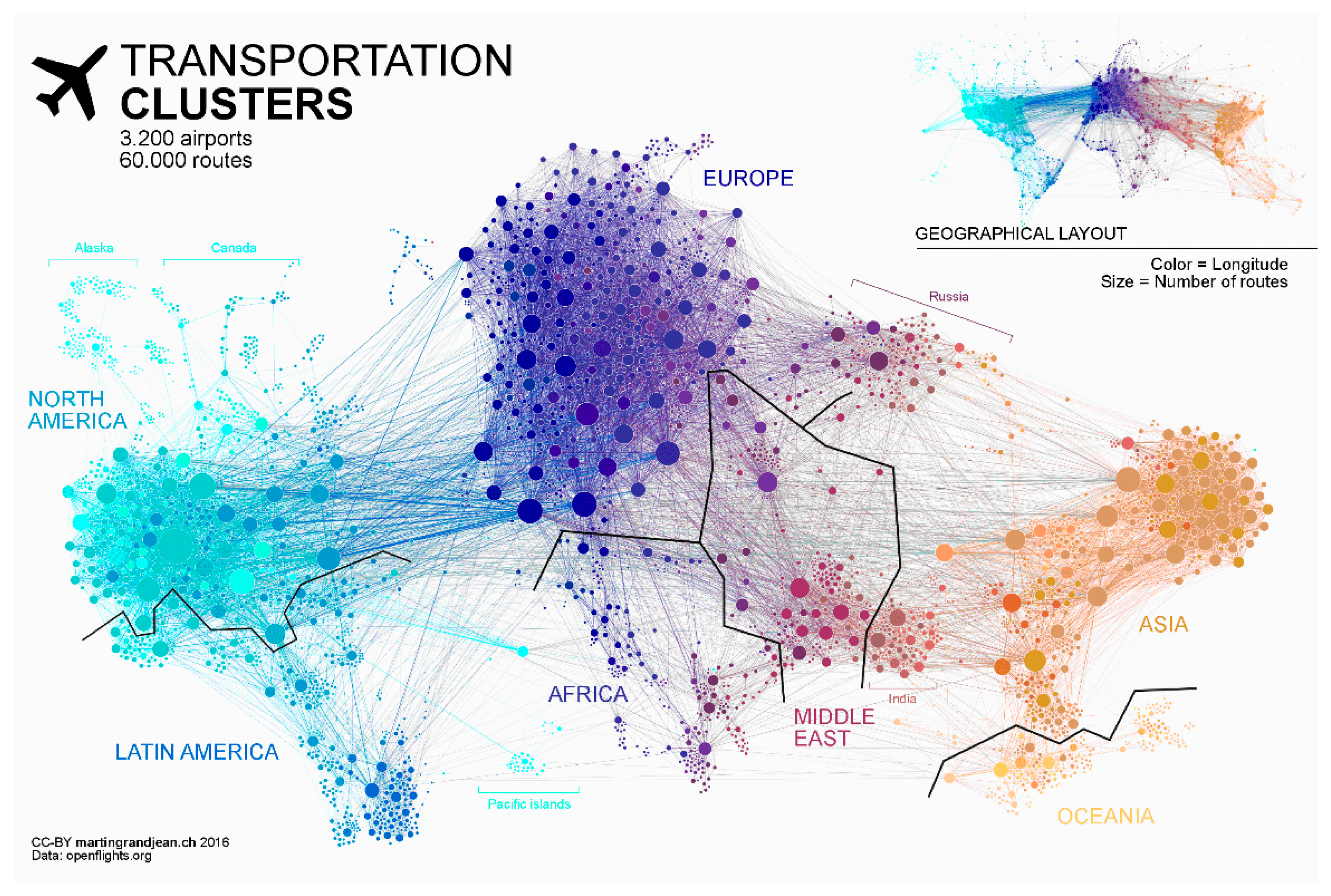
Figure 2.
Methodology of time series system represented with transfer entropy graph model.
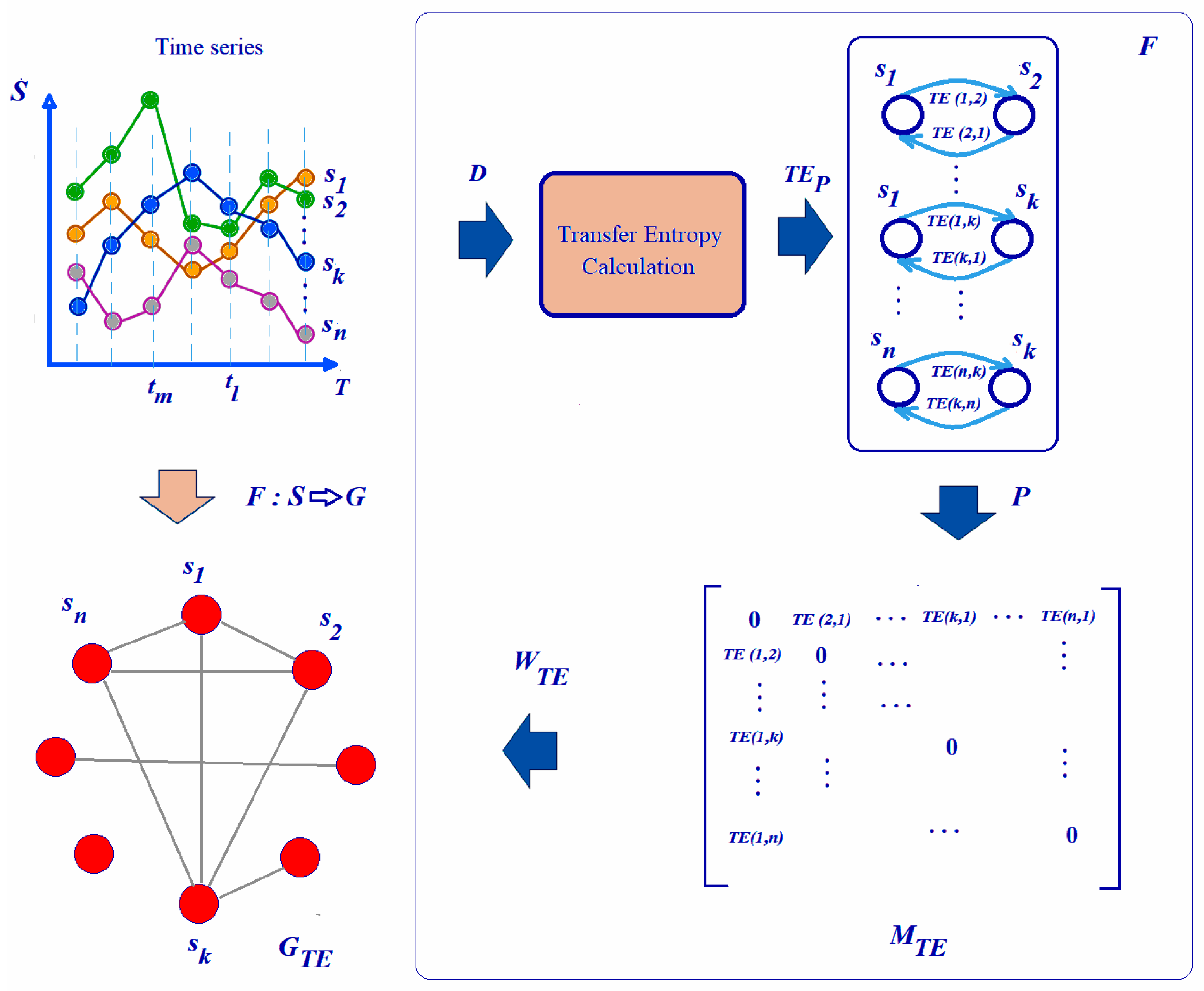
Figure 3.
Air transport statistics on cargo [29].
Figure 3.
Air transport statistics on cargo [29].
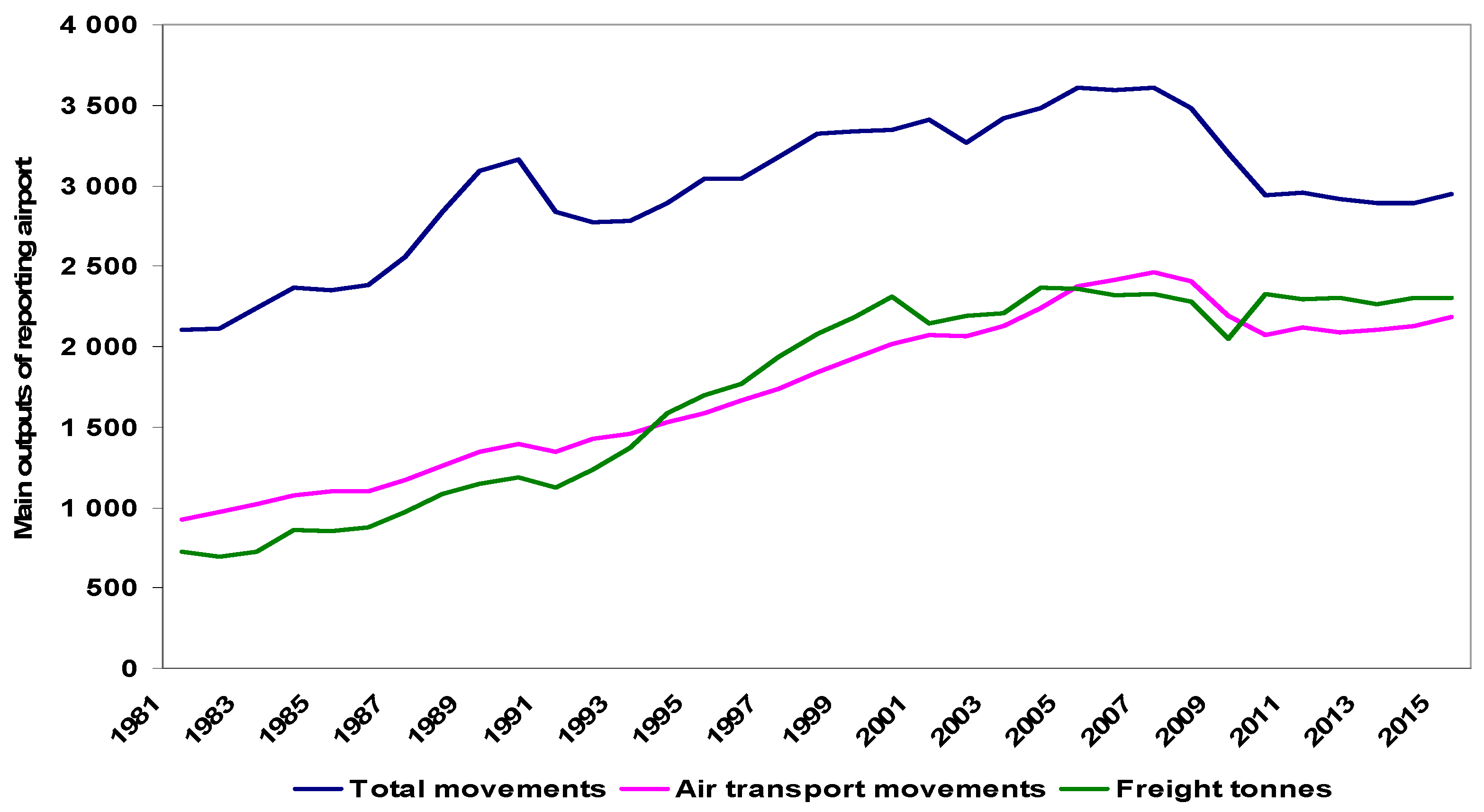
Figure 4.
Air transport statistics on passengers [29].
Figure 4.
Air transport statistics on passengers [29].
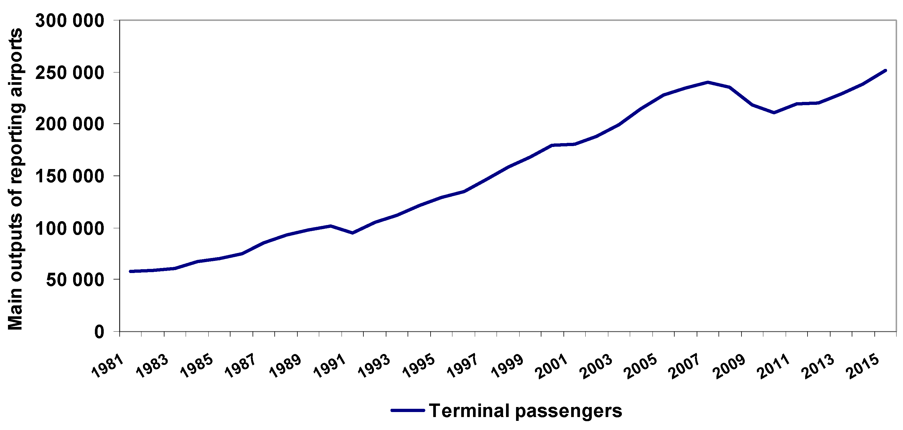
Figure 5.
Graphs GTE (a) and GTES (b) for movements, passengers and fright statistics.
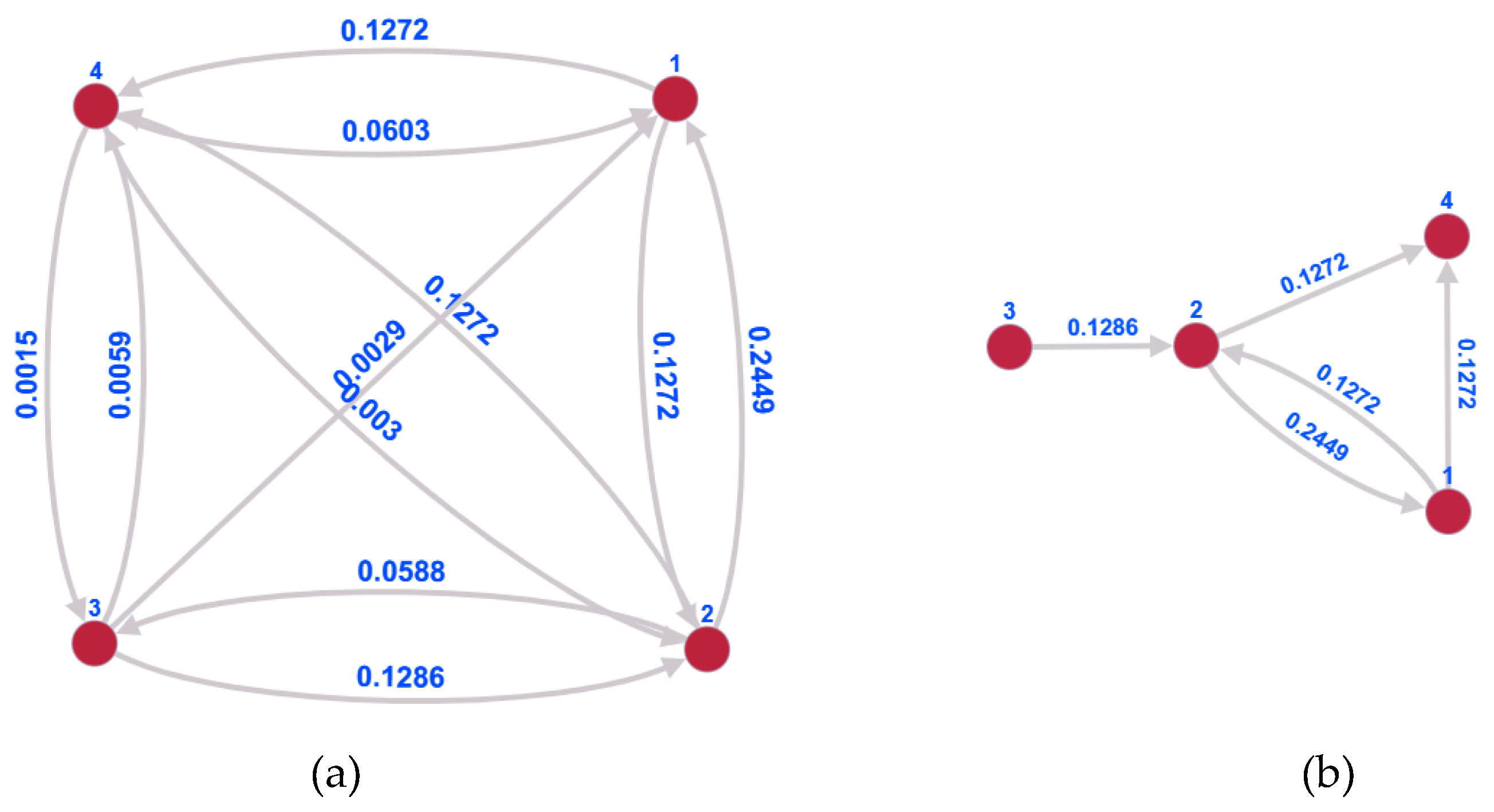
Figure 6.
Passengers flow for 2018 [30].
Figure 6.
Passengers flow for 2018 [30].
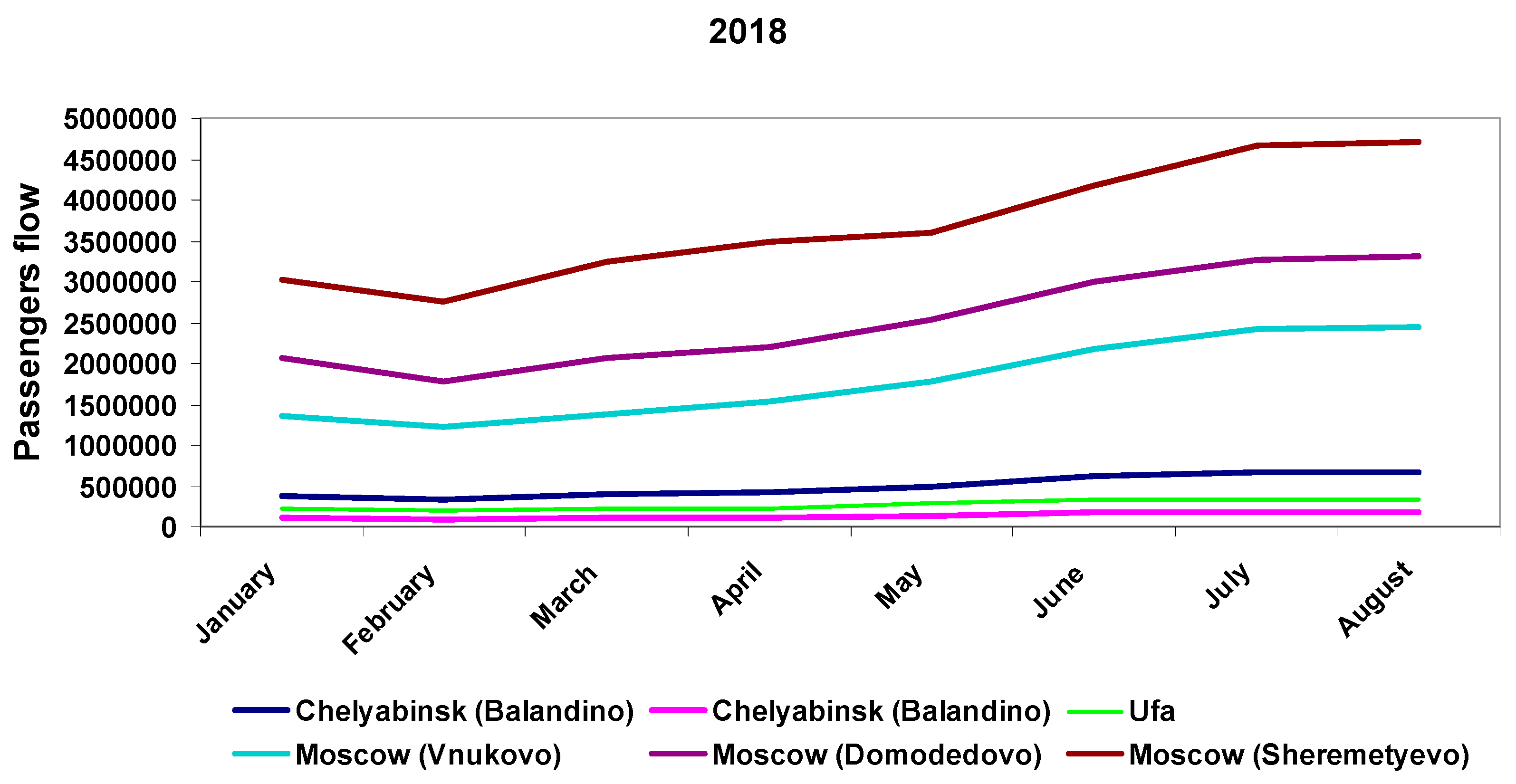
Figure 7.
Freight flow for 2018 [30].
Figure 7.
Freight flow for 2018 [30].
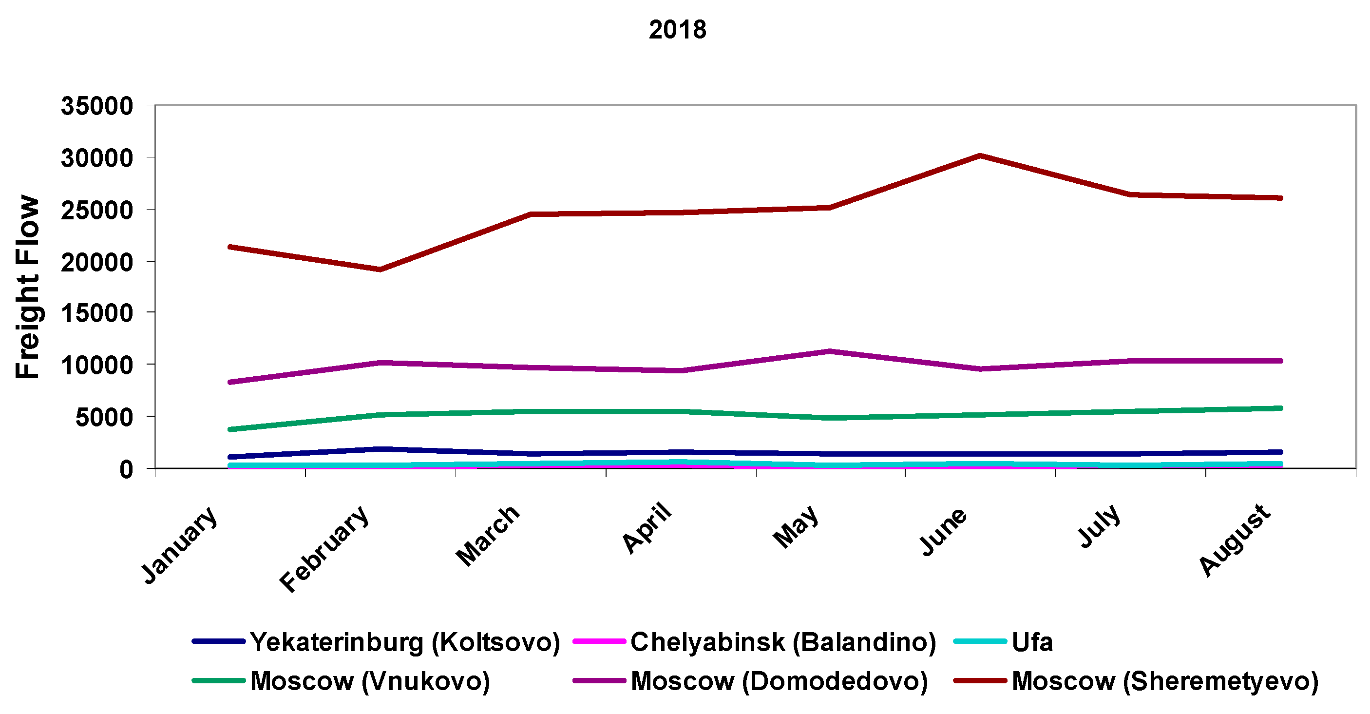
Figure 8.
Graph GTE for total movement, air transport movements: (a) Terminal passengers; (b) freight.
Figure 8.
Graph GTE for total movement, air transport movements: (a) Terminal passengers; (b) freight.
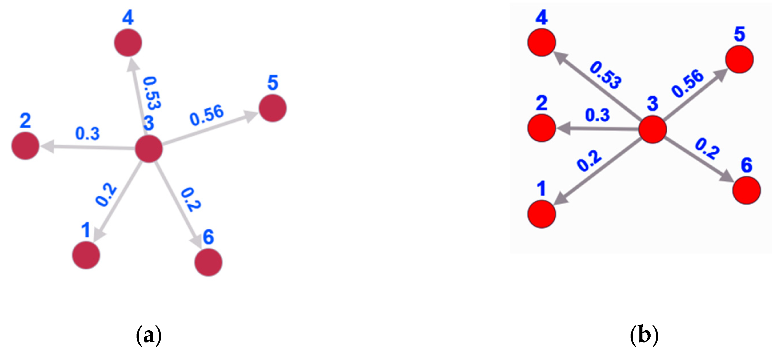
Figure 9.
ICAO Statistical regions [32].
Figure 9.
ICAO Statistical regions [32].
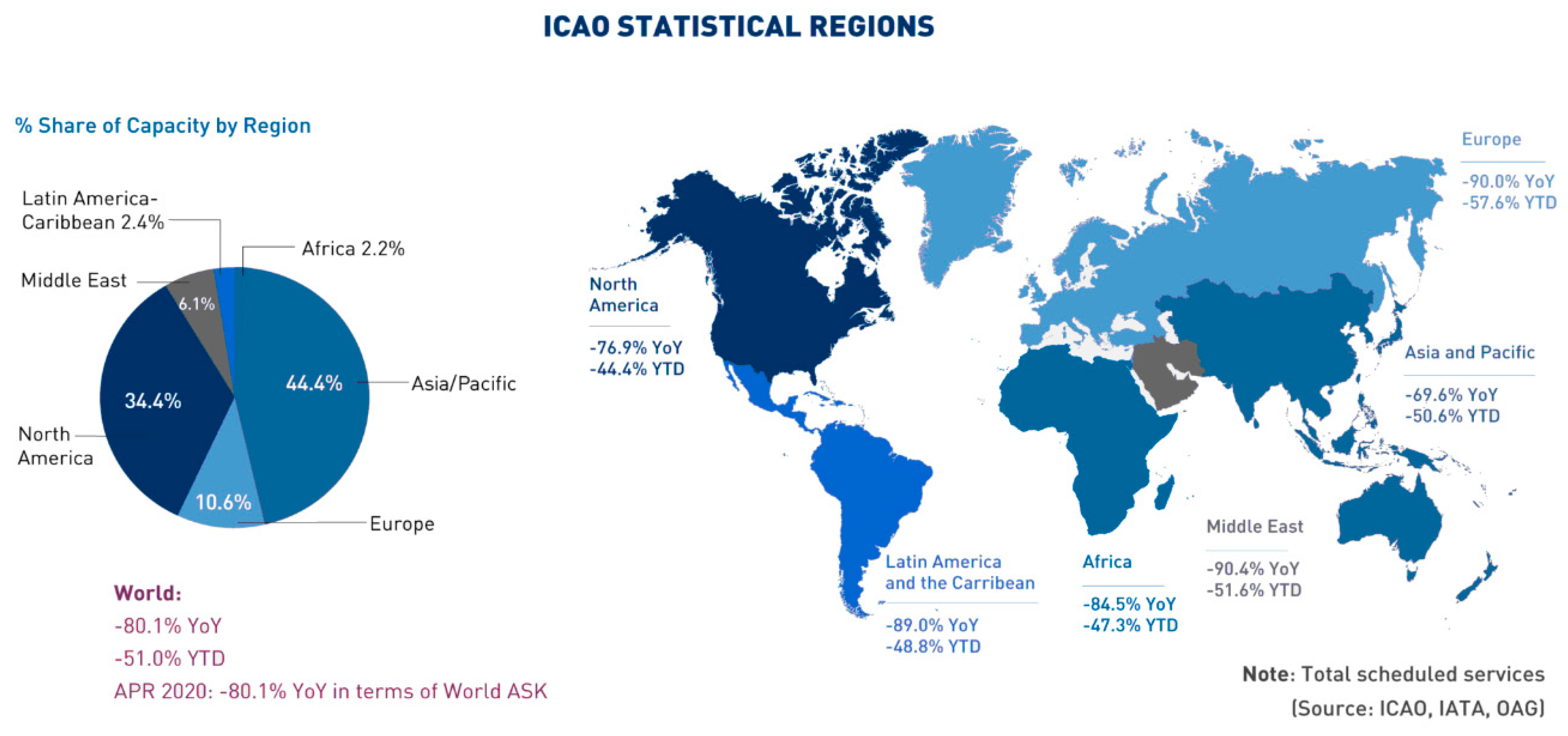
Figure 10.
Plot describing the change in the flow of passenger air traffic in the world for the period 1970-2021 years [33].
Figure 10.
Plot describing the change in the flow of passenger air traffic in the world for the period 1970-2021 years [33].
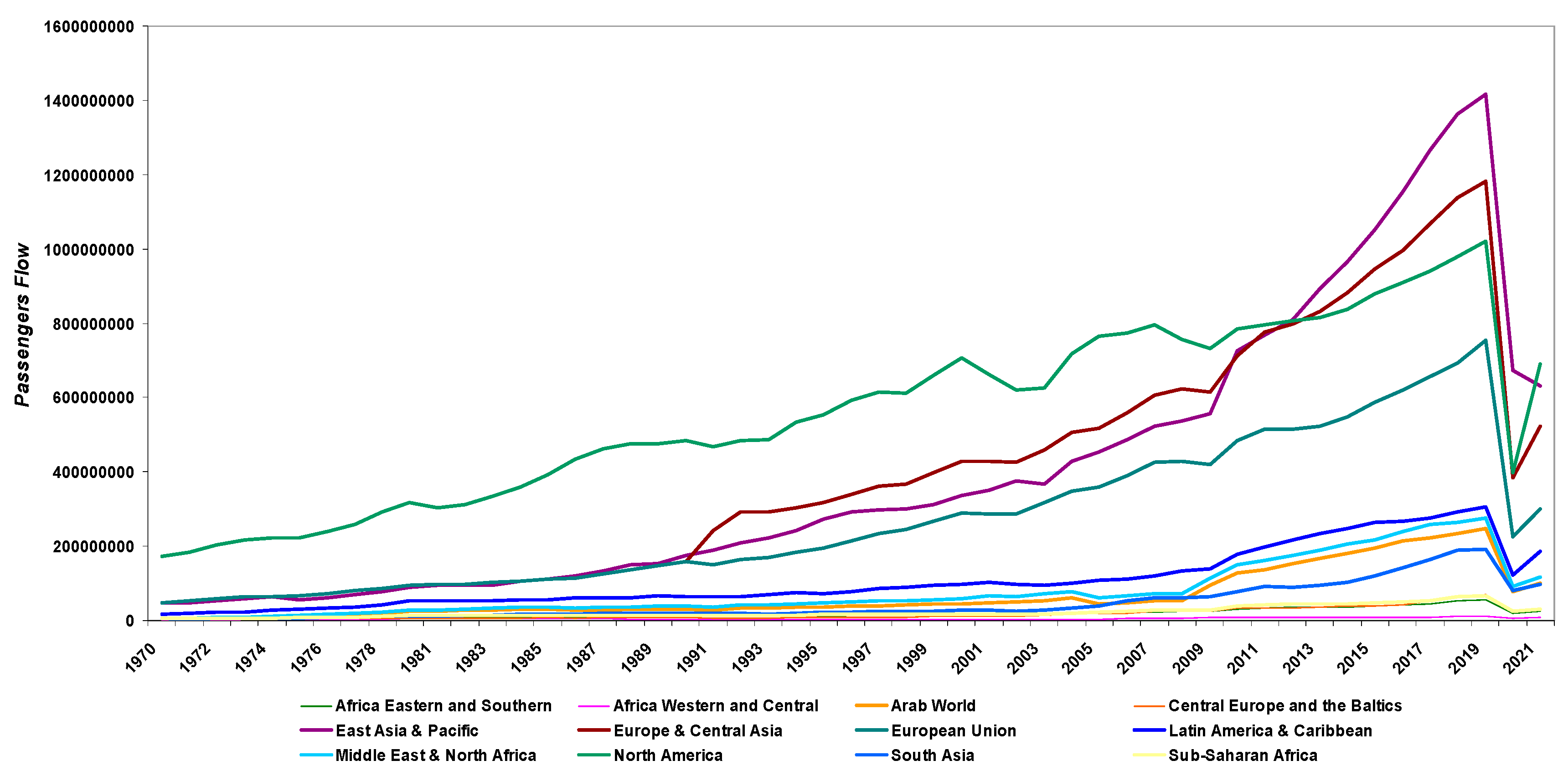
Figure 11.
TE graph for 1970-1980.
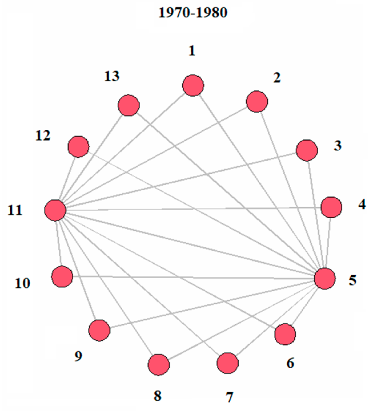
Figure 12.
TE graph for 1980-1990.
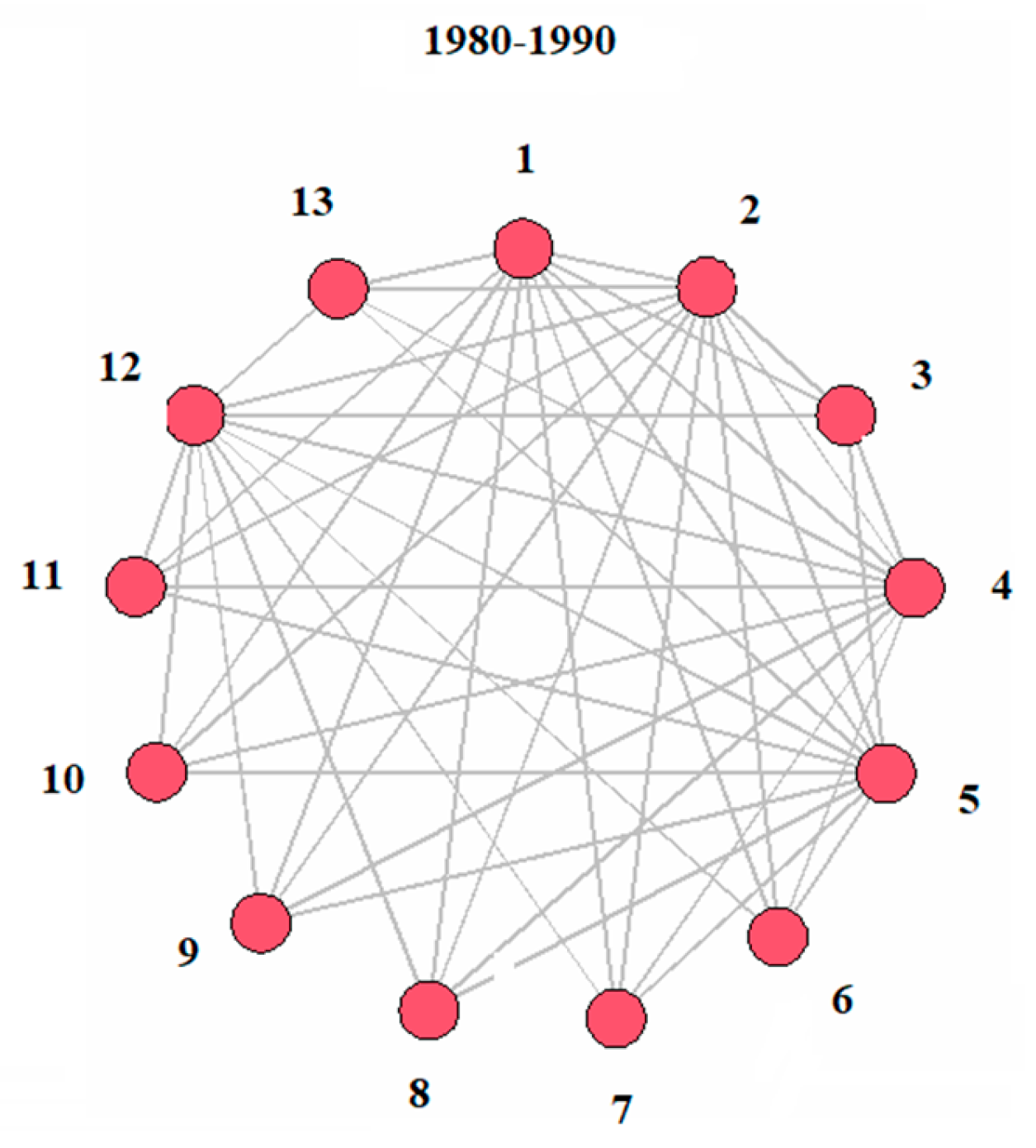
Figure 13.
TE graph for 1991-2000.
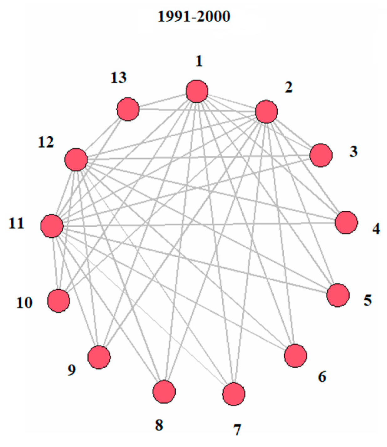
Figure 14.
TE graph for 2001-2010.
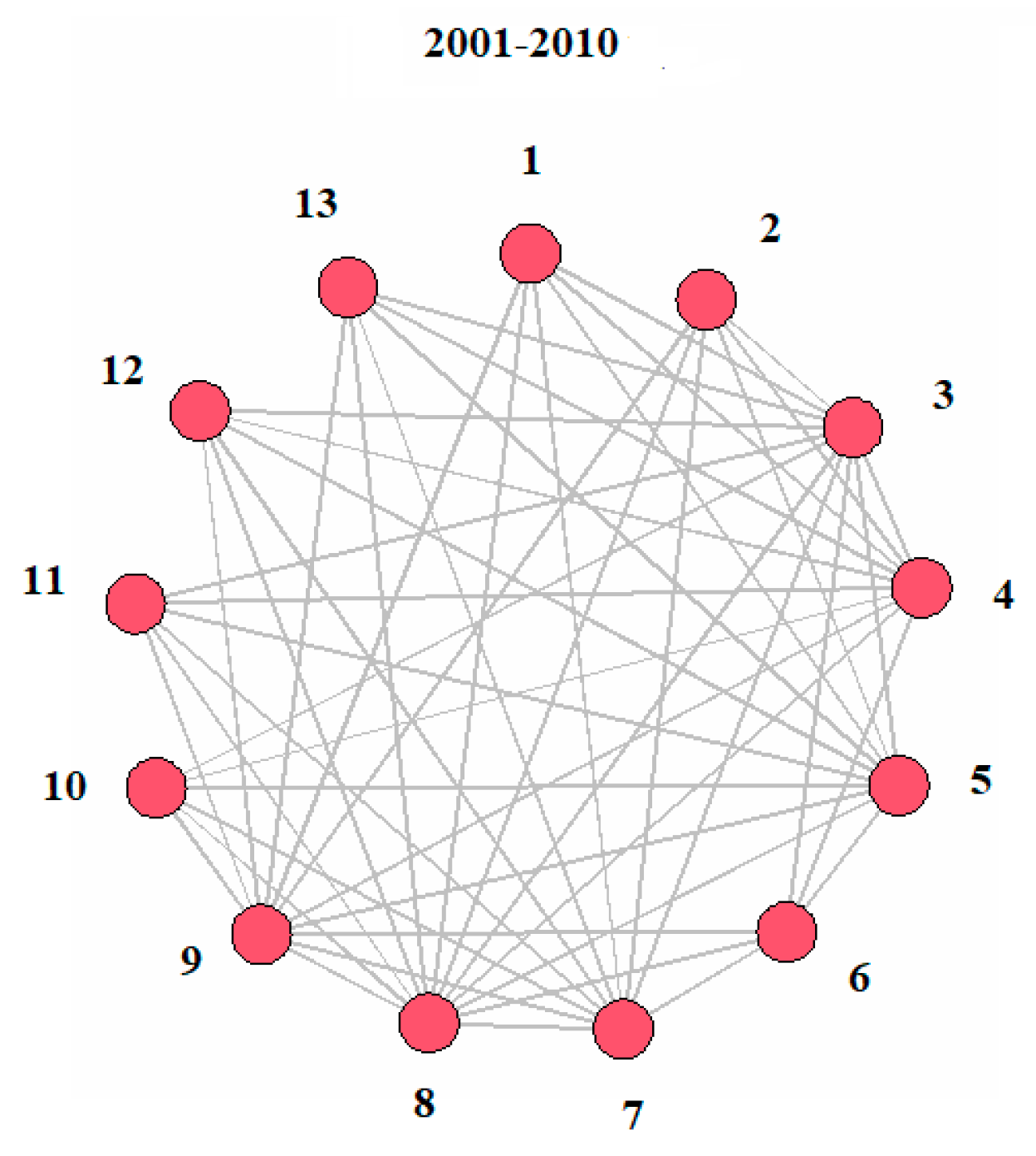
Figure 15.
TE graph for 2011-2021.
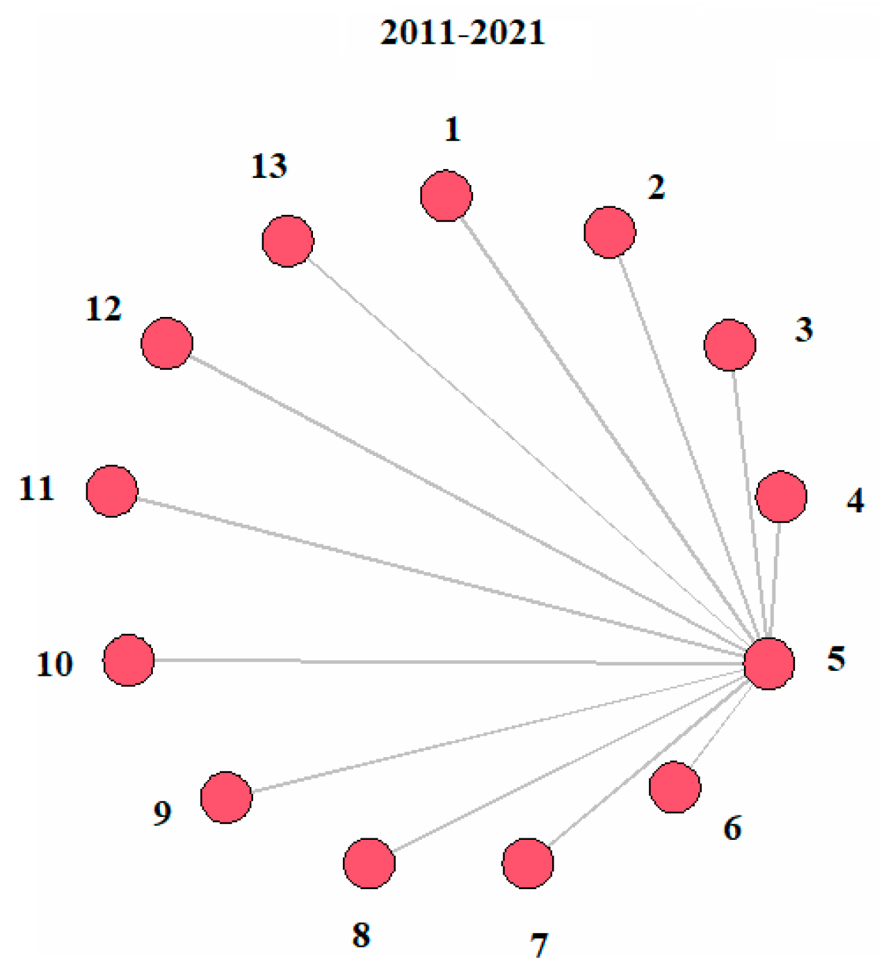
Figure 16.
TE graph for 1970-2021.
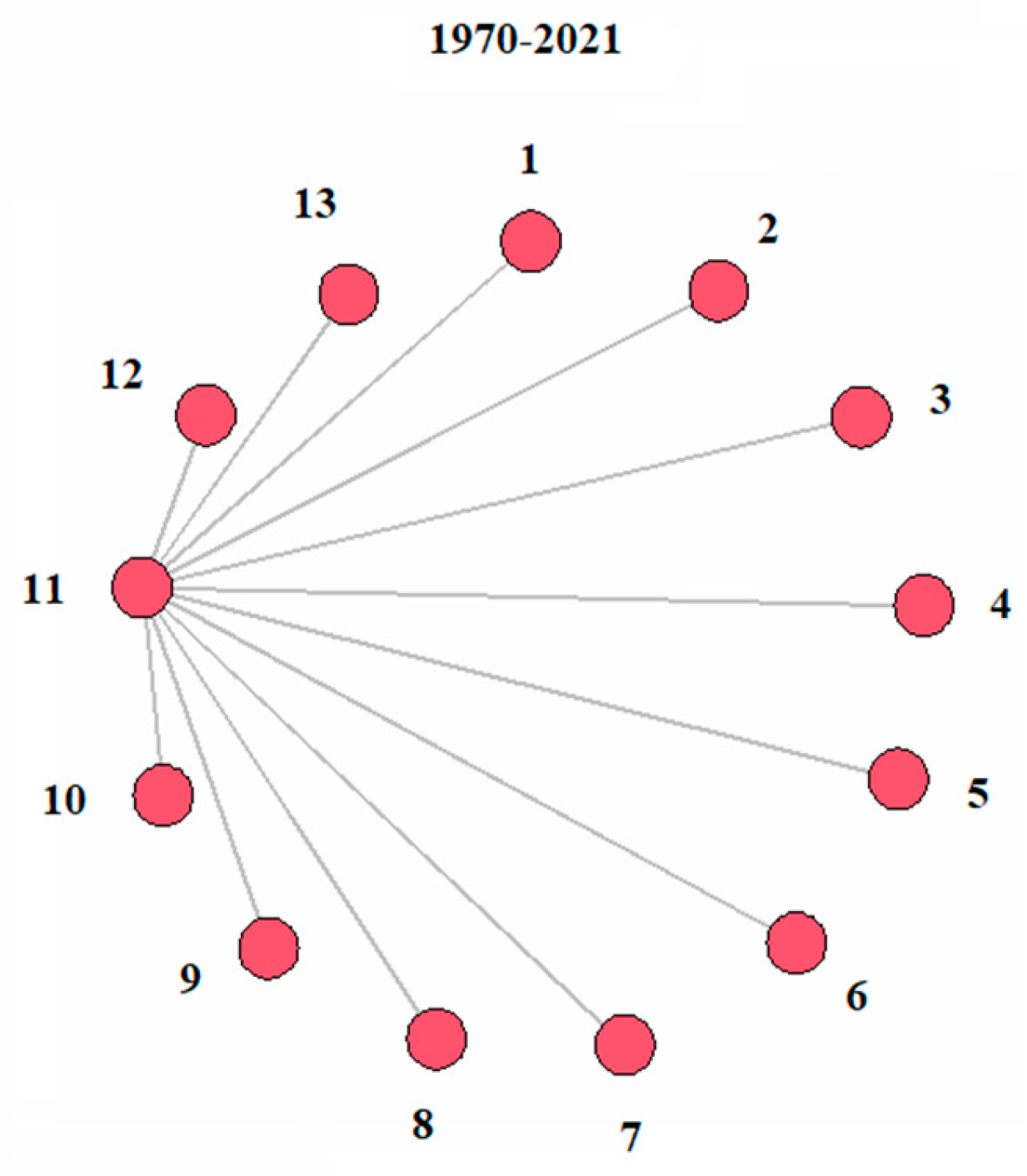
Figure 17.
TE graph for 2006-2015.
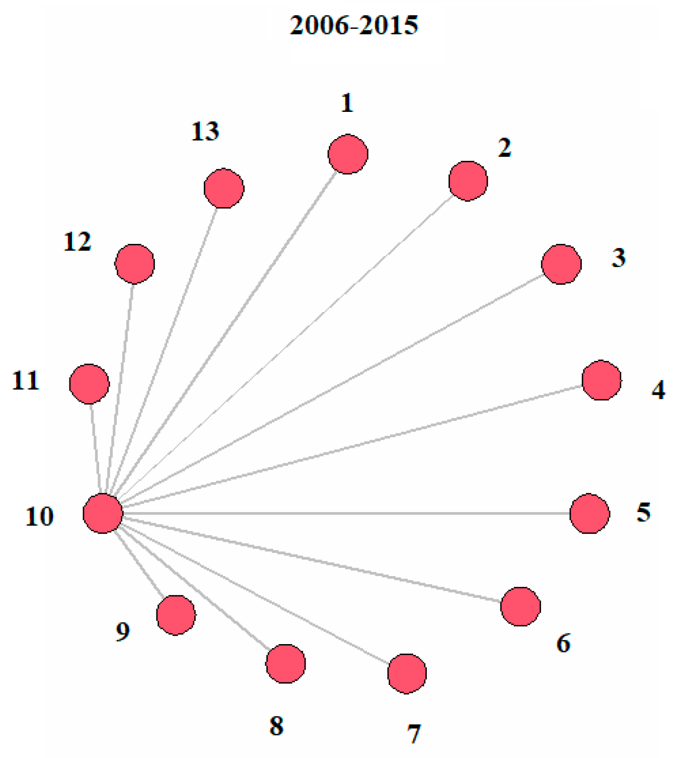
Figure 18.
Plot describing the change in the flow of passenger air transport in the world for the period 2001-2010 [33].
Figure 18.
Plot describing the change in the flow of passenger air transport in the world for the period 2001-2010 [33].
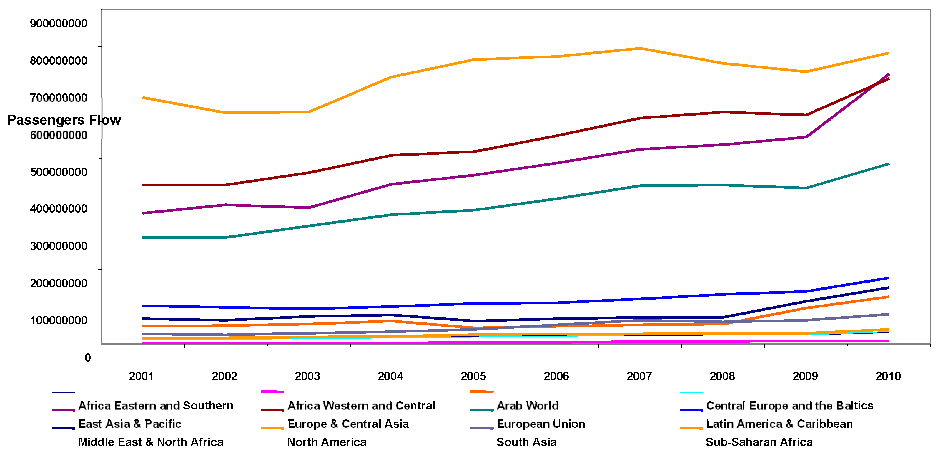
Figure 19.
GTE and maximum flow for different pairs regions for the period 2001-2010: (a) GTE without Max Flows analysis; (b) Max Flow from Source: SSA to Sink: EU; (c) Max Flow from Source: SSA to Sink: LA&C; (d) Max Flow from Source: SSA to Sink: AW&C.
Figure 19.
GTE and maximum flow for different pairs regions for the period 2001-2010: (a) GTE without Max Flows analysis; (b) Max Flow from Source: SSA to Sink: EU; (c) Max Flow from Source: SSA to Sink: LA&C; (d) Max Flow from Source: SSA to Sink: AW&C.
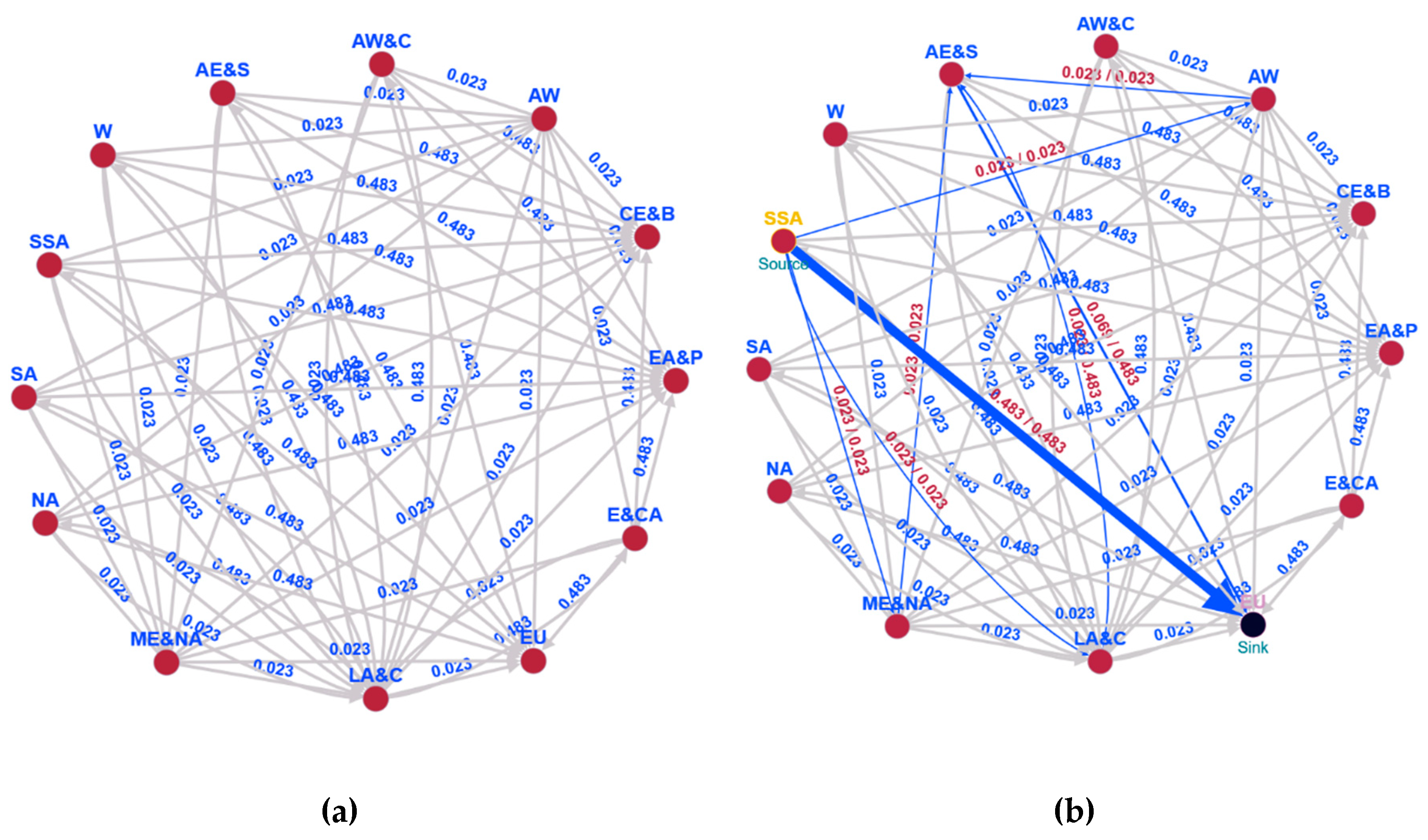
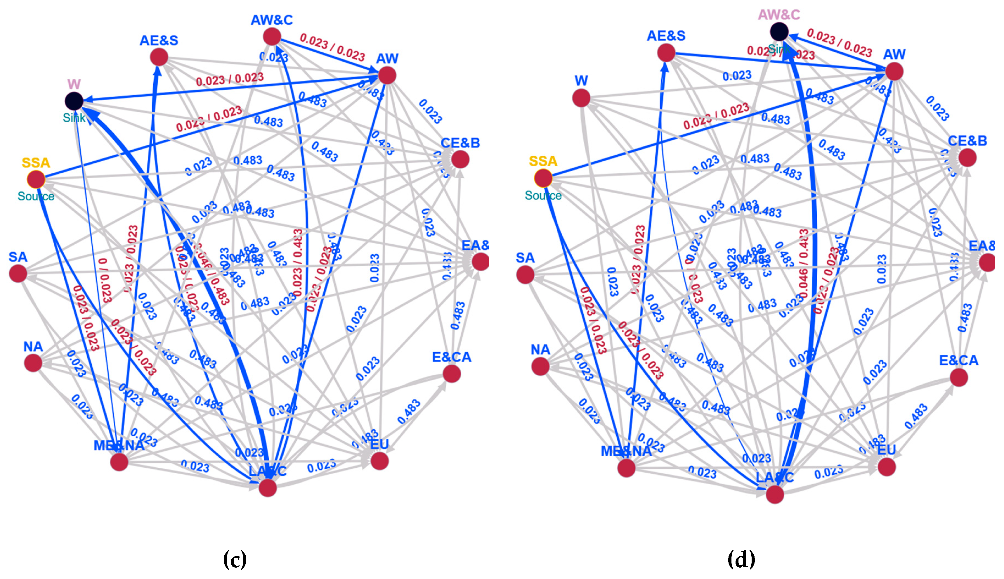

Table 1.
Transfer entropy from Y to X based on movements, passengers and fright statistics.
| Y | X | |||
|---|---|---|---|---|
| Total Movements |
Air Transport Movements | Terminal Passengers |
Fright Tonnes |
|
| Total Movements | 0 | 0.13 | 0 | 0.13 |
| Air Transport Movements | 0.25 | 0 | 0 | 0.13 |
| Terminal Passengers | 0 | 0.13 | 0 | 0 |
| Fright Tonnes | 0 | 0 | 0 | 0 |
Table 2.
Transfer entropy from Y to X based on regional transportation statistics.
| Y | X | |||||
|---|---|---|---|---|---|---|
| Yekaterinburg | Chelyabinsk | Ufa | Moscow (Vnukovo) |
Moscow (Domodedovo) |
Moscow (Sheremetyevo) |
|
| Yekaterinburg | 0 | 0 | 0.4 / 0 | 0 | 0 | 0 |
| Chelyabinsk | 0 | 0 | 0 | 0 | 0 | 0 |
| Ufa | 0 / 0.2 | 0 / 0.3 | 0 | 0.3 / 0.53 | 0.3 / 0.56 | 0.5 / 0.2 |
| Moscow (Vnukovo) | 0 | 0 | 0 | 0 | 0 | 0 |
| Moscow (Domodedovo) | 0 | 0 | 0 | 0 | 0 | 0 |
| Moscow (Sheremetyevo) | 0 | 0 | 0 | 0 | 0 | 0 |
Table 3.
Transfer entropy values for 1970-2021.
| 1970-1921 | 1 | 2 | 3 | 4 | 5 | 6 | 7 | 8 | 9 | 10 | 11 | 12 | 13 |
|---|---|---|---|---|---|---|---|---|---|---|---|---|---|
| Africa Eastern and Southern | Africa Western and Central | Arab World | Central Europe and the Baltics | East Asia & Pacific | Europe & Central Asia | European Union | Latin America & Caribbean | Middle East & North Africa | North America | South Asia | Sub-Saharan Africa | World | |
| Africa Eastern and Southern | 0 | 0 | 0 | 0 | 0 | 0 | 0 | 0 | 0 | 0 | 0.18 | 0 | 0 |
| Africa Western and Central | 0 | 0 | 0 | 0 | 0 | 0 | 0 | 0 | 0 | 0 | 0.18 | 0 | 0 |
| Arab World | 0 | 0 | 0 | 0 | 0 | 0 | 0 | 0 | 0 | 0 | 0.18 | 0 | 0 |
| Central Europe and the Baltics | 0 | 0 | 0 | 0 | 0 | 0 | 0 | 0 | 0 | 0 | 0.18 | 0 | 0 |
| East Asia & Pacific | 0 | 0 | 0 | 0 | 0 | 0 | 0 | 0 | 0 | 0 | 0.18 | 0 | 0 |
| Europe & Central Asia | 0 | 0 | 0 | 0 | 0 | 0 | 0 | 0 | 0 | 0 | 0.18 | 0 | 0 |
| European Union | 0 | 0 | 0 | 0 | 0 | 0 | 0 | 0 | 0 | 0 | 0.18 | 0 | 0 |
| Latin America & Caribbean | 0 | 0 | 0 | 0 | 0 | 0 | 0 | 0 | 0 | 0 | 0.18 | 0 | 0 |
| Middle East & North Africa | 0 | 0 | 0 | 0 | 0 | 0 | 0 | 0 | 0 | 0 | 0.18 | 0 | 0 |
| North America | 0 | 0 | 0 | 0 | 0 | 0 | 0 | 0 | 0 | 0 | 0.18 | 0 | 0 |
| South Asia | 0.04 | 0.04 | 0.04 | 0.04 | 0 | 0.04 | 0 | 0.04 | 0.04 | 0.04 | 0 | 0.04 | 0 |
| Sub-Saharan Africa | 0 | 0 | 0 | 0 | 0 | 0 | 0 | 0 | 0 | 0 | 0.18 | 0 | 0 |
| World | 0 | 0 | 0 | 0 | 0 | 0 | 0 | 0 | 0 | 0 | 0.18 | 0 | 0 |
Table 4.
Transfer entropy values for 1970-2080.
| 1970-1980 | 1 | 2 | 3 | 4 | 5 | 6 | 7 | 8 | 9 | 10 | 11 | 12 | 13 |
|---|---|---|---|---|---|---|---|---|---|---|---|---|---|
| Africa Eastern and Southern | Africa Western and Central | Arab World | Central Europe and the Baltics | East Asia & Pacific | Europe & Central Asia | European Union | Latin America & Caribbean | Middle East & North Africa | North America | South Asia | Sub-Saharan Africa | World | |
| Africa Eastern and Southern | 0 | 0 | 0 | 0 | 0.2 | 0 | 0 | 0 | 0 | 0 | 0.45 | 0 | 0 |
| Africa Western and Central | 0 | 0 | 0 | 0 | 0.2 | 0 | 0 | 0 | 0 | 0 | 0.45 | 0 | 0 |
| Arab World | 0 | 0 | 0 | 0 | 0.2 | 0 | 0 | 0 | 0 | 0 | 0.45 | 0 | 0 |
| Central Europe and the Baltics | 0 | 0 | 0 | 0 | 0.2 | 0 | 0 | 0 | 0 | 0 | 0.45 | 0 | 0 |
| East Asia & Pacific | 0 | 0 | 0 | 0 | 0 | 0 | 0 | 0 | 0 | 0 | 0.45 | 0 | 0 |
| Europe & Central Asia | 0 | 0 | 0 | 0 | 0.2 | 0 | 0 | 0 | 0 | 0 | 0.45 | 0 | 0 |
| European Union | 0 | 0 | 0 | 0 | 0.2 | 0 | 0 | 0 | 0 | 0 | 0.45 | 0 | 0 |
| Latin America & Caribbean | 0 | 0 | 0 | 0 | 0.2 | 0 | 0 | 0 | 0 | 0 | 0.45 | 0 | 0 |
| Middle East & North Africa | 0 | 0 | 0 | 0 | 0.2 | 0 | 0 | 0 | 0 | 0 | 0.45 | 0 | 0 |
| North America | 0 | 0 | 0 | 0 | 0.2 | 0 | 0 | 0 | 0 | 0 | 0.45 | 0 | 0 |
| South Asia | 0 | 0 | 0 | 0 | 0.2 | 0 | 0 | 0 | 0 | 0 | 0 | 0 | 0 |
| Sub-Saharan Africa | 0 | 0 | 0 | 0 | 0.2 | 0 | 0 | 0 | 0 | 0 | 0.45 | 0 | 0 |
| World | 0 | 0 | 0 | 0 | 0.2 | 0 | 0 | 0 | 0 | 0 | 0.45 | 0 | 0 |
Table 5.
Transfer entropy values for 1981-1990.
| 1981-1990 | 1 | 2 | 3 | 4 | 5 | 6 | 7 | 8 | 9 | 10 | 11 | 12 | 13 |
|---|---|---|---|---|---|---|---|---|---|---|---|---|---|
| Africa Eastern and Southern | Africa Western and Central | Arab World | Central Europe and the Baltics | East Asia & Pacific | Europe & Central Asia | European Union | Latin America & Caribbean | Middle East & North Africa | North America | South Asia | Sub-Saharan Africa | World | |
| Africa Eastern and Southern | 0 | 0.02 | 0 | 0.02 | 0 | 0 | 0 | 0 | 0 | 0 | 0 | 0 | 0 |
| Africa Western and Central | 0 | 0 | 0 | 0 | 0 | 0 | 0 | 0 | 0 | 0 | 0 | 0 | 0 |
| Arab World | 0.23 | 0.02 | 0 | 0.48 | 0.5 | 0 | 0 | 0 | 0 | 0 | 0 | 0.023 | 0 |
| Central Europe and the Baltics | 0.23 | 0.02 | 0 | 0 | 0 | 0 | 0 | 0 | 0 | 0 | 0 | 0.023 | 0 |
| East Asia & Pacific | 0.23 | 0.02 | 0 | 0 | 0 | 0 | 0 | 0 | 0 | 0 | 0 | 0.023 | 0 |
| Europe & Central Asia | 0.23 | 0.02 | 0 | 0.48 | 0.5 | 0 | 0 | 0 | 0 | 0 | 0 | 0.023 | 0 |
| European Union | 0.23 | 0.02 | 0 | 0.48 | 0.5 | 0 | 0 | 0 | 0 | 0 | 0 | 0.023 | 0 |
| Latin America & Caribbean | 0.23 | 0.02 | 0 | 0.48 | 0.5 | 0 | 0 | 0 | 0 | 0 | 0 | 0.023 | 0 |
| Middle East & North Africa | 0.23 | 0.02 | 0 | 0.48 | 0.5 | 0 | 0 | 0 | 0 | 0 | 0 | 0.023 | 0 |
| North America | 0.23 | 0.02 | 0 | 0.48 | 0.5 | 0 | 0 | 0 | 0 | 0 | 0 | 0.023 | 0 |
| South Asia | 0.23 | 0.02 | 0 | 0.48 | 0.5 | 0 | 0 | 0 | 0 | 0 | 0 | 0.023 | 0 |
| Sub-Saharan Africa | 0 | 0.02 | 0 | 0.48 | 0 | 0 | 0 | 0 | 0 | 0 | 0 | 0 | 0 |
| World | 0.23 | 0.02 | 0 | 0.48 | 0.5 | 0 | 0 | 0 | 0 | 0 | 0 | 0.023 | 0 |
Table 6.
Transfer entropy values for 1991-2000.
| 1991-2000 | 1 | 2 | 3 | 4 | 5 | 6 | 7 | 8 | 9 | 10 | 11 | 12 | 13 |
|---|---|---|---|---|---|---|---|---|---|---|---|---|---|
| Africa Eastern and Southern | Africa Western and Central | Arab World | Central Europe and the Baltics | East Asia & Pacific | Europe & Central Asia | European Union | Latin America & Caribbean | Middle East & North Africa | North America | South Asia | Sub-Saharan Africa | World | |
| Africa Eastern and Southern | 0 | 0.48 | 0 | 0 | 0 | 0 | 0 | 0 | 0 | 0 | 0.483 | 0 | 0 |
| Africa Western and Central | 0.02 | 0 | 0 | 0 | 0 | 0 | 0 | 0 | 0 | 0 | 0.023 | 0.023 | 0 |
| Arab World | 0.48 | 0.02 | 0 | 0 | 0 | 0 | 0 | 0 | 0 | 0 | 0.023 | 0.483 | 0 |
| Central Europe and the Baltics | 0.48 | 0.02 | 0 | 0 | 0 | 0 | 0 | 0 | 0 | 0 | 0.023 | 0.483 | 0 |
| East Asia & Pacific | 0.48 | 0.02 | 0 | 0 | 0 | 0 | 0 | 0 | 0 | 0 | 0.023 | 0.483 | 0 |
| Europe & Central Asia | 0.48 | 0.02 | 0 | 0 | 0 | 0 | 0 | 0 | 0 | 0 | 0.023 | 0.483 | 0 |
| European Union | 0.48 | 0.02 | 0 | 0 | 0 | 0 | 0 | 0 | 0 | 0 | 0.023 | 0.483 | 0 |
| Latin America & Caribbean | 0.48 | 0.02 | 0 | 0 | 0 | 0 | 0 | 0 | 0 | 0 | 0.023 | 0.483 | 0 |
| Middle East & North Africa | 0.48 | 0.02 | 0 | 0 | 0 | 0 | 0 | 0 | 0 | 0 | 0.023 | 0.483 | 0 |
| North America | 0.48 | 0.02 | 0 | 0 | 0 | 0 | 0 | 0 | 0 | 0 | 0.023 | 0.483 | 0 |
| South Asia | 0.02 | 0 | 0 | 0 | 0 | 0 | 0 | 0 | 0 | 0 | 0 | 0.023 | 0 |
| Sub-Saharan Africa | 0 | 0.48 | 0 | 0 | 0 | 0 | 0 | 0 | 0 | 0 | 0.483 | 0 | 0 |
| World | 0.48 | 0.02 | 0 | 0 | 0 | 0 | 0 | 0 | 0 | 0 | 0.023 | 0.483 | 0 |
Table 7.
Transfer entropy values for 2001-2010.
| 2001-2010 | 1 | 2 | 3 | 4 | 5 | 6 | 7 | 8 | 9 | 10 | 11 | 12 | 13 |
|---|---|---|---|---|---|---|---|---|---|---|---|---|---|
| Africa Eastern and Southern | Africa Western and Central | Arab World | Central Europe and the Baltics | East Asia & Pacific | Europe & Central Asia | European Union | Latin America & Caribbean | Middle East & North Africa | North America | South Asia | Sub-Saharan Africa | World | |
| Africa Eastern and Southern | 0 | 0 | 0.02 | 0 | 0 | 0 | 0 | 0.48 | 0.02 | 0 | 0 | 0 | 0 |
| Africa Western and Central | 0 | 0 | 0.02 | 0 | 0 | 0 | 0 | 0.48 | 0.02 | 0 | 0 | 0 | 0 |
| Arab World | 0.02 | 0.02 | 0 | 0 | 0 | 0.02 | 0 | 0.02 | 0 | 0.02 | 0.023 | 0.023 | 0 |
| Central Europe and the Baltics | 0.48 | 0.48 | 0.02 | 0 | 0 | 0.48 | 0 | 0.02 | 0.02 | 0.48 | 0.483 | 0.483 | 0.5 |
| East Asia & Pacific | 0.48 | 0.48 | 0.02 | 0 | 0 | 0.48 | 0 | 0.02 | 0.02 | 0.48 | 0.483 | 0.483 | 0.5 |
| Europe & Central Asia | 0 | 0 | 0.02 | 0 | 0 | 0 | 0 | 0.48 | 0.02 | 0 | 0 | 0 | 0 |
| European Union | 0.48 | 0.48 | 0.02 | 0 | 0 | 0.48 | 0 | 0.02 | 0.02 | 0.48 | 0.483 | 0.483 | 0.5 |
| Latin America & Caribbean | 0.02 | 0.02 | 0.02 | 0 | 0 | 0.02 | 0 | 0 | 0.02 | 0.02 | 0.023 | 0.023 | 0 |
| Middle East & North Africa | 0.02 | 0.02 | 0 | 0 | 0 | 0.02 | 0 | 0.02 | 0 | 0.02 | 0.023 | 0.023 | 0 |
| North America | 0 | 0 | 0.02 | 0 | 0 | 0 | 0 | 0.48 | 0.02 | 0 | 0 | 0 | 0 |
| South Asia | 0 | 0 | 0.02 | 0 | 0 | 0 | 0 | 0.48 | 0.02 | 0 | 0 | 0 | 0 |
| Sub-Saharan Africa | 0 | 0 | 0.02 | 0 | 0 | 0 | 0 | 0.48 | 0.02 | 0 | 0 | 0 | 0 |
| World | 0 | 0 | 0.02 | 0 | 0 | 0 | 0 | 0.48 | 0.02 | 0 | 0 | 0 | 0 |
Table 8.
Transfer entropy values for 2011-2021.
| 2011-2021 | 1 | 2 | 3 | 4 | 5 | 6 | 7 | 8 | 9 | 10 | 11 | 12 | 13 |
|---|---|---|---|---|---|---|---|---|---|---|---|---|---|
| Africa Eastern and Southern | Africa Western and Central | Arab World | Central Europe and the Baltics | East Asia & Pacific | Europe & Central Asia | European Union | Latin America & Caribbean | Middle East & North Africa | North America | South Asia | Sub-Saharan Africa | World | |
| Africa Eastern and Southern | 0 | 0 | 0 | 0 | 0.5 | 0 | 0 | 0 | 0 | 0 | 0 | 0 | 0 |
| Africa Western and Central | 0 | 0 | 0 | 0 | 0.5 | 0 | 0 | 0 | 0 | 0 | 0 | 0 | 0 |
| Arab World | 0 | 0 | 0 | 0 | 0.5 | 0 | 0 | 0 | 0 | 0 | 0 | 0 | 0 |
| Central Europe and the Baltics | 0 | 0 | 0 | 0 | 0.5 | 0 | 0 | 0 | 0 | 0 | 0 | 0 | 0 |
| East Asia & Pacific | 0 | 0 | 0 | 0 | 0 | 0 | 0 | 0 | 0 | 0 | 0 | 0 | 0 |
| Europe & Central Asia | 0 | 0 | 0 | 0 | 0.5 | 0 | 0 | 0 | 0 | 0 | 0 | 0 | 0 |
| European Union | 0 | 0 | 0 | 0 | 0.5 | 0 | 0 | 0 | 0 | 0 | 0 | 0 | 0 |
| Latin America & Caribbean | 0 | 0 | 0 | 0 | 0.5 | 0 | 0 | 0 | 0 | 0 | 0 | 0 | 0 |
| Middle East & North Africa | 0 | 0 | 0 | 0 | 0.5 | 0 | 0 | 0 | 0 | 0 | 0 | 0 | 0 |
| North America | 0 | 0 | 0 | 0 | 0.5 | 0 | 0 | 0 | 0 | 0 | 0 | 0 | 0 |
| South Asia | 0 | 0 | 0 | 0 | 0.5 | 0 | 0 | 0 | 0 | 0 | 0 | 0 | 0 |
| Sub-Saharan Africa | 0 | 0 | 0 | 0 | 0.5 | 0 | 0 | 0 | 0 | 0 | 0 | 0 | 0 |
| World | 0 | 0 | 0 | 0 | 0.5 | 0 | 0 | 0 | 0 | 0 | 0 | 0 | 0 |
Table 9.
Transfer entropy values for 2005-2016.
| 2005-2016 | 1 | 2 | 3 | 4 | 5 | 6 | 7 | 8 | 9 | 10 | 11 | 12 | 13 |
|---|---|---|---|---|---|---|---|---|---|---|---|---|---|
| Africa Eastern and Southern | Africa Western and Central | Arab World | Central Europe and the Baltics | East Asia & Pacific | Europe & Central Asia | European Union | Latin America & Caribbean | Middle East & North Africa | North America | South Asia | Sub-Saharan Africa | World | |
| Africa Eastern and Southern | 0 | 0 | 0 | 0 | 0 | 0 | 0 | 0 | 0 | 0.02 | 0 | 0 | 0 |
| Africa Western and Central | 0 | 0 | 0 | 0 | 0 | 0 | 0 | 0 | 0 | 0.02 | 0 | 0 | 0 |
| Arab World | 0 | 0 | 0 | 0 | 0 | 0 | 0 | 0 | 0 | 0.02 | 0 | 0 | 0 |
| Central Europe and the Baltics | 0 | 0 | 0 | 0 | 0 | 0 | 0 | 0 | 0 | 0.02 | 0 | 0 | 0 |
| East Asia & Pacific | 0 | 0 | 0 | 0 | 0 | 0 | 0 | 0 | 0 | 0.02 | 0 | 0 | 0 |
| Europe & Central Asia | 0 | 0 | 0 | 0 | 0 | 0 | 0 | 0 | 0 | 0.02 | 0 | 0 | 0 |
| European Union | 0 | 0 | 0 | 0 | 0 | 0 | 0 | 0 | 0 | 0.02 | 0 | 0 | 0 |
| Latin America & Caribbean | 0 | 0 | 0 | 0 | 0 | 0 | 0 | 0 | 0 | 0.02 | 0 | 0 | 0 |
| Middle East & North Africa | 0 | 0 | 0 | 0 | 0 | 0 | 0 | 0 | 0 | 0.02 | 0 | 0 | 0 |
| North America | 0 | 0 | 0 | 0 | 0 | 0 | 0 | 0 | 0 | 0 | 0 | 0 | 0 |
| South Asia | 0 | 0 | 0 | 0 | 0 | 0 | 0 | 0 | 0 | 0.02 | 0 | 0 | 0 |
| Sub-Saharan Africa | 0 | 0 | 0 | 0 | 0 | 0 | 0 | 0 | 0 | 0.02 | 0 | 0 | 0 |
| World | 0 | 0 | 0 | 0 | 0 | 0 | 0 | 0 | 0 | 0.02 | 0 | 0 | 0 |
Disclaimer/Publisher’s Note: The statements, opinions and data contained in all publications are solely those of the individual author(s) and contributor(s) and not of MDPI and/or the editor(s). MDPI and/or the editor(s) disclaim responsibility for any injury to people or property resulting from any ideas, methods, instructions or products referred to in the content. |
© 2024 by the authors. Licensee MDPI, Basel, Switzerland. This article is an open access article distributed under the terms and conditions of the Creative Commons Attribution (CC BY) license (https://creativecommons.org/licenses/by/4.0/).
Copyright: This open access article is published under a Creative Commons CC BY 4.0 license, which permit the free download, distribution, and reuse, provided that the author and preprint are cited in any reuse.


