Some Approximation Properties of Two Dimensional Chlodovsky-Bernstein Operators Based on (P, Q) Integer

1. Introduction

Approximation theory is fast becoming a key instrument not only in classical approximation theory but also in other fields of mathematics such as differential equations, orthogonal polynomials and geometric design. Since Korovkin’s famous theorem was first published in 1950, the issue of approximation by linear positive operators has became increasingly important area as part of approximation theory. A considerable amount of literature has been published on that [1,2,10,12,14,15,23,24].

In the past two decades, the applications of $q-$calculus in approximation theory have been studied extensively. Firstly, the Bernstein polynomials based on $q-$integers was done by Lupaş [6]. As approximation of $q-$Bernstein polynomials studied by Lupaş is better than classical one under convenient choice of q, many authors introduced q-generalization of many operators and examined several approximation properties. Several studies have revealed that [3,7,8,13].

In recent years, Mursaleen et al. have focused on $(p,q)$-calculus in approximate by linear positive operator and proposed $(p,q)-$analogue of Bernstein operators [20,21]. They computed uniform convergence of the operators and rate of convergence. For some recent study directed to $(p,q)$-operators, we can refer the readers to [17,18,19,26,27].

The main motivation in this paper, to the best of authors knowledge, no study about approximate two variable operator has been found so far using $(p,q)$ calculus. In the present study, we define the two dimensional Chlodovsky type Bernstein operators based on $(p,q)-$integer. We examine approximation properties of our new operator by the help of Korovkin-type theorem. In addition, we present the local approximation properties and establish the rates of convergence by means of the modulus of continuity and the Lipschitz type maximal function. Also, we give a Voronovskaja type theorem for this operators. Another important aim of this study is to examine weighted approximation properties of these our operators on ${\mathbb{R}}_{+}^2=[0,\infty )\times [0,\infty )$. In order to get these results, we will apply the weighted Korovkin type theorem.

Let us recall some definitions and notations regarding the concept of $(p,q)-$calculus. The $(p,q)-$integer of the number n is defined by

$${\left[n\right]}_{p,q}:={\displaystyle \frac{p^n-q^n}{p-q}},n=1,2,3\dots ,0<q<p\le 1.$$

The $(p,q)-$factorial ${\left[n\right]}_{p,q}!$ and the $(p,q)-$binomial coefficients are defined as :

$${\left[n\right]}_{p,q}!:=\left\{\begin{array}{cc}{\left[n\right]}_{p,q}{\left[n-1\right]}_{p,q}\cdots {\left[1\right]}_{p,q},\hfill & n\in \mathbb{N}\\ 1,\hfill & n=0\end{array}\right..$$

and

$${\left[\begin{array}{c}n\\ k\end{array}\right]}_{p,q}={\displaystyle \frac{{\left[n\right]}_{p,q}!}{{\left[k\right]}_{p,q}!{\left[n-k\right]}_{p,q}!}},0\le k\le n.$$

Further, the $(p,q)-$binomial expansions are given as

$${(ax+by)}_{p,q}^n=\sum _{k=0}^n{p}^{\left({\displaystyle \genfrac{}{}{0pt}{}{n-k}{2}}\right)}{q}^{\left({\displaystyle \genfrac{}{}{0pt}{}{k}{2}}\right)}{a}^{n-k}{b}^k{x}^{n-k}{y}^k.$$

and

$${(x-y)}_{p,q}^n=(x-y)(px-qy)(p^{2}x-q^{2}y)\cdots (p^{n-1}x-q^{n-1}y).$$

Further information related to $(p,q)-$calculus can be found in [25,28].

2. Construction of the Operators

Recently, Ansari and Karaisa [16] have defined and studied $(p,q)-$analogue of Chlodovsky operators as follows:

$$C_{n,p,q}\left(f;x\right)={\displaystyle \frac{1}{p^{n(n-1)/2}}}\sum _{k=0}^n{\left[\begin{array}{c}n\\ k\end{array}\right]}_{p,q}{p}^{k(k-1)/2}{\left({\displaystyle \frac{x}{b_n}}\right)}^k{\left(1-{\displaystyle \frac{x}{b_n}}\right)}_{p,q}^{n-k-1}f\left({\displaystyle \frac{{\left[k\right]}_{p,q}}{{\left[n\right]}_{p,q}{p}^{k-n}}}{b}_n\right),$$

(1)

where

$${\left(1-{\displaystyle \frac{x}{b_n}}\right)}_{p,q}^{n-k-1}=\prod _{s=0}^{n-k-1}\left(p^s-q^s{\displaystyle \frac{x}{b_n}}\right).$$

For $0<q_1,q_2<p_1,p_2\le 1$, we define Chlodovsky type two dimensional Bernstein operator based on $(p,q)-$integers as follows:

$$C_{n,m}^{(p_1,q_1),(p_1,q_1)}\left(f;x,y\right)=\sum _{k=0}^n\sum _{j=0}^m{\mathrm{\Phi }}_{n,k}(p_1,q_1;x){\mathrm{\Phi }}_{m,j}(p_2,q_2;y)f\left({\displaystyle \frac{{\left[k\right]}_{p_1,q_1}}{{\left[n\right]}_{p_1,q_1}{p}_1^{k-n}}}{\alpha }_n,{\displaystyle \frac{{\left[j\right]}_{p_2,q_2}}{{\left[m\right]}_{p_2,q_2}{p}_2^{j-m}}}{\beta }_m\right),$$

(2)

for all $n,m\in N$, $f\in C\left(I_{{\alpha }_n{\beta }_m}\right)$ with $I_{{\alpha }_n{\beta }_m}=\{(x,y):0\le {\alpha }_n\le x,0\le {\beta }_m\le y\}$ and $C\left(I_{{\alpha }_n{\beta }_m}\right)=\{f:I_{{\alpha }_n{\beta }_m}⟶R\mathrm{is}\mathrm{continuous}\}$. Here $\left({\alpha }_n\right)$ and $\left({\beta }_m\right)$ be increasing unbounded sequences of positive real numbers such that

$$\begin{array}{ccc}\hfill \underset{n\to \infty }{lim}{\displaystyle \frac{{\alpha }_n}{{\left[n\right]}_{p_1,q_1}}}& =& 0,\hfill \end{array}$$

(3)

$$\begin{array}{ccc}\hfill \underset{m\to \infty }{lim}{\displaystyle \frac{{\beta }_m}{{\left[m\right]}_{p_2,q_2}}}& =& 0.\hfill \end{array}$$

(4)

Also, the basis elements are

$$\begin{array}{ccc}\hfill {\mathrm{\Phi }}_{n,k}(p_1,q_1;x)& =& p_1^{{\displaystyle \frac{k(k-1)-n(n-1)}{2}}}{\left[\begin{array}{c}n\\ k\end{array}\right]}_{p_1,q_1}{\left({\displaystyle \frac{x}{{\alpha }_n}}\right)}^k\prod _{s=0}^{n-k-1}\left(p_1^s-q_1^s{\displaystyle \frac{x}{{\alpha }_n}}\right),\hfill \\ \hfill {\mathrm{\Phi }}_{m,j}(p_2,q_2;y)& =& p_2^{{\displaystyle \frac{j(j-1)-m(m-1)}{2}}}{\left[\begin{array}{c}m\\ j\end{array}\right]}_{p_2,q_2}{\left({\displaystyle \frac{y}{{\beta }_m}}\right)}^j\prod _{s=0}^{m-j-1}\left(p_2^s-q_2^s{\displaystyle \frac{y}{{\beta }_m}}\right).\hfill \end{array}$$

Now, we need following lemmas for proving our main results.

Lemma 1. [16] 

$$\begin{array}{ccc}\hfill C_{n,p,q}\left(1;x\right)& =& 1,\hfill \\ \hfill C_{n,p,q}\left(e_1;x\right)& =& x,\hfill \\ \hfill C_{n,p,q}\left(e_2;x\right)& =& {\displaystyle \frac{p^{n-1}{b}_n}{{\left[n\right]}_{p,q}}}x+{\displaystyle \frac{q{[n-1]}_{p,q}}{{\left[n\right]}_{p,q}}}{x}^2\hfill \\ \hfill C_{n,p,q}\left(e_3;x\right)& =& {\displaystyle \frac{b_n^{2}x}{{\left[n\right]}_{p,q}^2}}{p}^{2n-2}+{\displaystyle \frac{(2p+q)q{[n-1]}_{p,q}{x}^2{b}_n}{{\left[n\right]}_{p,q}^2}}{p}^{n-1}+{\displaystyle \frac{q^3{[n-1]}_{p,q}{[n-2]}_{p,q}{x}^3}{{\left[n\right]}_{p,q}^2}},\hfill \\ \hfill C_{n,p,q}\left(e_4;x\right)& =& {\displaystyle \frac{b_n^{3}x}{{\left[n\right]}_{p,q}^3}}{p}^{3n-3}+{\displaystyle \frac{q(3p^2+3qp+q^3){[n-1]}_{p,q}{b}_n^2{x}^2}{{\left[n\right]}_{p,q}^3}}{p}^{2n-4}\hfill \\ & & +{\displaystyle \frac{q^3(3p^2+2pq+q^2){[n-1]}_{p,q}{[n-2]}_{p,q}{b}_n{x}^3}{{\left[n\right]}_{p,q}^3}}{p}^{n-3}+{\displaystyle \frac{q^6{[n-1]}_{p,q}{[n-2]}_{p,q}{[n-3]}_{p,q}{x}^4}{{\left[n\right]}_{p,q}^3}}.\hfill \end{array}$$

From Lemma 1, we have following:

Lemma 2. 

$$\begin{array}{ccc}\hfill C_{n,m}^{(p_1,q_1),(p_2,q_2)}\left(1;x,y\right)& =& 1,\hfill \\ \hfill C_{n,m}^{(p_1,q_1),(p_2,q_2)}\left(s;x,y\right)& =& x,\hfill \\ \hfill C_{n,m}^{(p_1,q_1),(p_2,q_2)}\left(t;x,y\right)& =& y,\hfill \\ \hfill C_{n,m}^{(p_1,q_1),(p_2,q_2)}\left(st;x,y\right)& =& xy,\hfill \\ \hfill C_{n,m}^{(p_1,q_1),(p_2,q_2)}\left(s^2;x,y\right)& =& {\displaystyle \frac{p_1^{n-1}{\alpha }_n}{{\left[n\right]}_{p_1,q_1}}}x+{\displaystyle \frac{q_1{[n-1]}_{p_1,q_1}}{{\left[n\right]}_{p_1,q_1}}}{x}^2,\hfill \\ \hfill C_{n,m}^{(p_1,q_1),(p_2,q_2)}\left(t^2;x,y\right)& =& {\displaystyle \frac{p_2^{m-1}{\beta }_m}{{\left[m\right]}_{p_2,q_2}}}y+{\displaystyle \frac{q_2{[m-1]}_{p_2,q_2}}{{\left[m\right]}_{p_2,q_2}}}{y}^2.\hfill \end{array}$$

Using Lemma 2 and by linearity of $C_{n,m}^{(p_1,q_1),(p_2,q_2)}$, we have

Remark 1. 

$$\begin{array}{ccc}\hfill C_{n,m}^{(p_1,q_1),(p_2,q_2)}\left({(t-x)}^2;x,y\right)& =& {\displaystyle \frac{-p_1^{n-1}{x}^2}{{\left[n\right]}_{p_1,q_1}}}+{\displaystyle \frac{x{p}_1^{n-1}{\alpha }_n}{{\left[n\right]}_{p_1,q_1}}},\hfill \end{array}$$

(5)

$$\begin{array}{ccc}\hfill C_{n,m}^{(p_1,q_1),(p_2,q_2)}\left({(s-y)}^2;x,y\right)& =& {\displaystyle \frac{-p_2^{m-1}{y}^2}{{\left[m\right]}_{p_2,q_2}}}+{\displaystyle \frac{y{p}_2^{m-1}{\beta }_m}{{\left[m\right]}_{p_2,q_2}}}.\hfill \end{array}$$

(6)

Theorem 1. 

Let $q_1:=\left(q_{1,n}\right)$, $p_1:=\left(p_{1,n}\right)$, $q_2:=\left(q_{2,m}\right)$, $p_2:=\left(p_{2,m}\right)$ such that $0<q_{1,n},q_{2,m}<p_{1,n},p_{2,m}\le 1$. If

$$\begin{array}{c}\hfill \underset{n}{lim}{p}_{1,n}=1,\underset{n}{lim}{q}_{1,n}=1,\underset{m}{lim}{p}_{2,m}=1,\underset{m}{lim}{q}_{2,m}=1,\underset{n}{lim}{p}_{1,n}^n=a_1\mathrm{and}\underset{m}{lim}{p}_{1,m}^m=a_2,\end{array}$$

(7)

the sequence $C_{n,m}^{(p_1,q_1),(p_2,q_2)}\left(f;x,y\right)$ convergence uniformly to $f(x,y)$, on $[0,a]\times [0,b]=I_{ab}$ for each $f\in C\left(I_{ab}\right)$, where $a,b$ be reel numbers such that $a\le {\alpha }_n$, $b\le {\beta }_m$ and $C\left(I_{ab}\right)$ be the space of all real valued continuous function on $I_{ab}$ with the norm

$$\begin{array}{c}\hfill {\Vert f\Vert }_{C\left(I_{ab}\right)}=\underset{(x,y)\in I_{ab}}{sup}\left|f(x,y)\right|.\end{array}$$

Proof. 

Assume that the equities (7),(3) and (4) are holds. Then, we have

$$\begin{array}{c}\hfill {\displaystyle \frac{p_{1,n}^{n-1}{\alpha }_n}{{\left[n\right]}_{p_{1,n},q_{1,n}}}}\to 0,{\displaystyle \frac{p_{2,m}^{m-1}{\beta }_m}{{\left[m\right]}_{p_{2,m},q_{2,m}}}}\to 0,{\displaystyle \frac{q_{1,n}{\left[n\right]}_{p_{1,n},q_{1,n}}}{{\left[n\right]}_{p_{1,n},q_{1,n}}}}\to 1\mathrm{and}{\displaystyle \frac{q_{2,m}{\left[m-1\right]}_{p_{2,m},q_{2,m}}}{{\left[m\right]}_{p_{2,m},q_{2,m}}}}\to 1.\end{array}$$

as $n,m⟶\infty$. From Lemma 2, we obtain ${lim}_{n,m\to \infty }{C}_{n,m}^{(p_1,q_1),(p_2,q_2)}\left(e_{ij};x,y\right)=e_{ij}(x,y)$ uniformly on $I_{ab}$, where $e_{ij}(x,y)=x^i{y}^j,0\le i+j\le 2$ are the test functions. By Korovkin’s theorem for functions of two variables was presented by Volkov [29], it follows that ${lim}_{n,m\to \infty }{C}_{n,m}^{(p_1,q_1),(p_2,q_2)}\left(f;x,y\right)=f(x,y)$, uniformly on $I_{ab}$, for each $f\in C\left(I_{ab}\right)$. □

3. Rate of Convergence

In this section, we compute the rates of convergence of operators $C_{n,m}^{(p_1,q_1),(p_2,q_2)}$ to $f(x,y)$ by means of the modulus of continuity. Proceeding further, we provide a summary of the notations and definitions of the modulus of continuity and the Peetre’s $K-$functional for bivariate real valued functions.

For $f\in C\left(I_{ab}\right)$, the complete modulus of continuity for a bivariate case is defined as follows:

$$\omega (f,\delta )=sup\left\{|f(t,s)-f(x,y)|:\sqrt{{(t-x)}^2+{(s-y)}^2}\le \delta \right\}.$$

for every $(t,s),(x,y)\in I_{ab}$. Further, partial moduli of continuity with respect to x and y are defined as

$$\begin{array}{ccc}\hfill {\omega }^1(f,\delta )& =& sup\left\{|f(x_1,y)-f(x_2,y)|:y\in [0,b]\mathrm{and}|x_1-x_2|\le \delta \right\}\hfill \\ \hfill {\omega }^2(f,\delta )& =& sup\left\{|f(x,y_1)-f(x,y_2)|:x\in [0,a]\mathrm{and}|y_1-y_2|\le \delta \right\},\hfill \end{array}$$

It is obvious that they satisfy the properties of the usual modulus of continuity [11].

For $\delta >0$, the Peetre-K functional [22] is given by

$$\begin{array}{c}\hfill K(f,\delta )=\underset{g\in C^2\left(I_{ab}\right)}{inf}\left\{{\parallel f-g\parallel }_{C\left(I_{ab}\right)}+\delta {\parallel g\parallel }_{C^2\left(I_{ab}\right)}\right\},\end{array}$$

where $C^2\left(I_{ab}\right)$ is the space of functions of f such that f, ${\displaystyle \frac{{\partial }^{j}f}{\partial x^j}}$ and ${\displaystyle \frac{{\partial }^{j}f}{\partial y^j}}$$(j=1,2)$ in $C\left(I_{ab}\right)$. The norm $\parallel .\parallel$ on the space $C^2\left(I_{ab}\right)$ is defined by

$$\begin{array}{c}\hfill {\parallel f\parallel }_{C^2{I}_{ab}}={\parallel f\parallel }_{C\left(I_{ab}\right)}+\sum _{j=1}^2\left({∥{\displaystyle \frac{{\partial }^{j}f}{\partial y^j}}∥}_{C\left(I_{ab}\right)}+{∥{\displaystyle \frac{{\partial }^{j}f}{\partial y^j}}∥}_{C\left(I_{ab}\right)}\right).\end{array}$$

Now, we give an estimate of the rate of convergence of operators $C_{n,m}^{(p_1,q_1),(p_2,q_2)}$.

Theorem 2. 

Let $f\in C\left(I_{ab}\right)$. For all $x\in I_{ab}$, we have

$$\left|C_{n,m}^{(p_1,q_1),(p_2,q_2)}-f\left(x,y\right)\right|\le 2\omega \left(f;{\delta }_{n,m}\right),$$

where

$$\begin{array}{ccc}\hfill {\delta }_{n,m}^2& =& {\displaystyle \frac{a{\alpha }_n{p}_1^{n-1}}{{\left[n\right]}_{p_1,q_1}}}+{\displaystyle \frac{b{\beta }_m{p}_2^{m-1}}{{\left[m\right]}_{p_2,q_2}}}.\hfill \end{array}$$

Proof. 

By definition the complete modulus of continuity of $f(x,y)$ and linearity and positivity our operator, we can write

$$\begin{array}{ccc}\hfill |C_{n,m}^{(p_1,q_1),(p_2,q_2)}\left(f;x,y\right)-f(x,y)|& \le & C_{n,m}^{(p_1,q_1),(p_2,q_2)}\left(\left|f\right(t,s)-f(x,y\left)\right|;x,y\right)\hfill \\ & \le & C_{n,m}^{(p_1,q_1),(p_2,q_2)}\left(\omega \left(f;\sqrt{{(t-x)}^2+{(s-y)}^2}\right);x,y\right)\hfill \\ & \le & \omega (f,{\delta }_{n,m})\left[{\displaystyle \frac{1}{{\delta }_{n,m}}}{C}_{n,m}^{(p_1,q_1),(p_2,q_2)}\left(\sqrt{{(t-x)}^2+{(s-y)}^2};x,y\right)\right].\hfill \end{array}$$

Using Cauchy-Scwartz inequality, from (5) and (6), one can write following

$$\begin{array}{ccc}& & |C_{n,m}^{(p_1,q_1),(p_2,q_2)}\left(f;x,y\right)-f(x,y)|\hfill \\ & \le & \omega (f,{\delta }_{n,m})\left[1+{\displaystyle \frac{1}{{\delta }_{n,m}}}{\left\{C_{n,m}^{(p_1,q_1),(p_2,q_2)}\left({(t-x)}^2+{(s-y)}^2;x,y\right)\right\}}^{1/2}\right]\hfill \\ & =& \omega (f,{\delta }_{n,m})\left[1+{\displaystyle \frac{1}{{\delta }_{n,m}}}{\left\{C_{n,m}^{(p_1,q_1),(p_2,q_2)}\left({(t-x)}^2;x,y\right)+C_{n,m}^{(p_1,q_1),(p_2,q_2)}\left({(s-y)}^2;x,y\right)\right\}}^{1/2}\right]\hfill \\ & \le & \omega (f,{\delta }_{n,m})\left[1+{\displaystyle \frac{1}{{\delta }_{n,m}}}{\left({\displaystyle \frac{a{\alpha }_n{p}_1^{n-1}}{{\left[n\right]}_{p_1,q_1}}}+{\displaystyle \frac{b{\beta }_m{p}_2^{m-1}}{{\left[m\right]}_{p_2,q_2}}}\right)}^{1/2}\right].\hfill \end{array}$$

Choosing ${\delta }_{n,m}={\left({\displaystyle \frac{a{\alpha }_n{p}_1^{n-1}}{{\left[n\right]}_{p_1,q_1}}}+{\displaystyle \frac{b{\beta }_m{p}_2^{m-1}}{{\left[m\right]}_{p_2,q_2}}}\right)}^{1/2}$, for all $(x,y)\in I_{ab}$, we get desired the result.

□

Theorem 3. 

Let $f\in C\left(I_{ab}\right)$, then the following inequalities satisfy

$$\left|C_{n,m}^{(p_1,q_1),(p_2,q_2)}-f\left(x,y\right)\right|\le {\omega }^1\left(f;{\delta }_n\right)+{\omega }^2\left(f;{\delta }_m\right),$$

where

$$\begin{array}{ccc}\hfill {\delta }_n^2& =& {\displaystyle \frac{a{\alpha }_n{p}_1^{n-1}}{{\left[n\right]}_{p_1,q_1}}},\hfill \end{array}$$

(8)

$$\begin{array}{ccc}\hfill {\delta }_m^2& =& {\displaystyle \frac{b{\beta }_m{p}_2^{m-1}}{{\left[m\right]}_{p_2,q_2}}}.\hfill \end{array}$$

(9)

Proof. 

By definition partial moduli of continuity of $f(x,y)$ and applying Cauchy-Scwartz inequality, we have

$$\begin{array}{ccc}\hfill |C_{n,m}^{(p_1,q_1),(p_2,q_2)}\left(f;x,y\right)-f(x,y)|& \le & C_{n,m}^{(p_1,q_1),(p_2,q_2)}\left(\left|f\right(t,s)-f(x,y\left)\right|;x,y\right)\hfill \\ & \le & C_{n,m}^{(p_1,q_1),(p_2,q_2)}\left(\left|f\right(t,s)-f(x,s\left)\right|;x,y\right)+C_{n,m}^{(p_1,q_1),(p_2,q_2)}\left(\left|f\right(x,s)-f(x,y\left)\right|;x,y\right)\hfill \\ & \le & C_{n,m}^{(p_1,q_1),(p_2,q_2)}\left(|{\omega }^1(f;|t-x\left|\right)|;x,y\right)+C_{n,m}^{(p_1,q_1),(p_2,q_2)}\left(|{\omega }^2(f;|s-y\left|\right)|;x,y\right)\hfill \\ & \le & {\omega }^1(f,{\delta }_n)\left[1+{\displaystyle \frac{1}{{\delta }_n}}{C}_{n,m}^{(p_1,q_1),(p_2,q_2)}\left(|t-x|;x,y\right)\right]\hfill \\ & & +{\omega }^2(f,{\delta }_m)\left[1+{\displaystyle \frac{1}{{\delta }_m}}{C}_{n,m}^{(p_1,q_1),(p_2,q_2)}\left(|s-y|;x,y\right)\right]\hfill \\ & \le & {\omega }^1(f,{\delta }_n)\left[1+{\displaystyle \frac{1}{{\delta }_n}}{\left(C_{n,m}^{(p_1,q_1),(p_2,q_2)}\left({(t-x)}^2;x,y\right)\right)}^{1/2}\right]\hfill \\ & & +{\omega }^2(f,{\delta }_m)\left[1+{\displaystyle \frac{1}{{\delta }_m}}{\left(C_{n,m}^{(p_1,q_1),(p_2,q_2)}\left({(s-y)}^2;x,y\right)\right)}^{1/2}\right].\hfill \end{array}$$

Consider (5), (6) and choosing

$$\begin{array}{ccc}\hfill {\delta }_n^2& =& {\displaystyle \frac{a{\alpha }_n{p}_1^{n-1}}{{\left[n\right]}_{p_1,q_1}}},\hfill \\ \hfill {\delta }_m^2& =& {\displaystyle \frac{b{\beta }_m{p}_2^{m-1}}{{\left[m\right]}_{p_2,q_2}}}.\hfill \end{array}$$

we reach the result. □

For ${\widehat{\alpha }}_1,{\widehat{\alpha }}_2\in (0,1]$ and $(s,t),(x,y)\in I_{ab}$, we define the Lipschitz class $LipM({\widehat{\alpha }}_1,{\widehat{\alpha }}_2)$ for the bivariate case as follows:

$$\begin{array}{c}\hfill \left|f(s,t)-f(x,y)\right|\le M{\left|s-x\right|}^{{\widehat{\alpha }}_1}{\left|t-y\right|}^{{\widehat{\alpha }}_2}.\end{array}$$

Theorem 4. 

Let $f\in Li{p}_M({\widehat{\alpha }}_1,{\widehat{\alpha }}_2)$. Then, for all $(x,y)\in I_{ab}$, we have

$$|C_{n,m}^{(p_1,q_1),(p_2,q_2)}\left(f;x,y\right)-f(x,y)|\le M{\delta }_n^{{\widehat{\alpha }}_1/2}{\delta }_m^{{\widehat{\alpha }}_2/2},$$

where ${\delta }_n$ and ${\delta }_m$ defined in (8) and (9), respectively.

Proof. 

As $f\in Li{p}_M({\widehat{\alpha }}_1,{\widehat{\alpha }}_2)$, it follows

$$\begin{array}{ccc}\hfill |C_{n,m}^{(p_1,q_1),(p_2,q_2)}\left(f;x,y\right)-f(x,y)|& \le & C_{n,m}^{(p_1,q_1),(p_2,q_2)}\left(\right|f(t,s)-f(x,y)|,q_n;x,y)\hfill \\ & \le & M{C}_{n,m}^{(p_1,q_1),(p_2,q_2)}{\left(\right|t-x|}^{{\widehat{\alpha }}_1}{|s-y|}^{{\widehat{\alpha }}_2};x,y)\hfill \\ & =& M{C}_{n,m}^{(p_1,q_1),(p_2,q_2)}{\left(\right|t-x|}^{{\widehat{\alpha }}_1}|;x)C_{n,m}^{(p_1,q_1),(p_2,q_2)}{\left(\right|s-y|}^{{\widehat{\alpha }}_2};y).\hfill \end{array}$$

For $\widehat{p}={\displaystyle \frac{1}{{\widehat{\alpha }}_1}},\widehat{q}={\displaystyle \frac{{\widehat{\alpha }}_1}{2-{\widehat{\alpha }}_1}}$ and $\widehat{p}={\displaystyle \frac{1}{{\widehat{\alpha }}_2}},\widehat{q}={\displaystyle \frac{{\widehat{\alpha }}_2}{2-{\widehat{\alpha }}_2}}$ applying the Hölder’s inequality, we get

$$\begin{array}{ccc}\hfill |C_{n,m}^{(p_1,q_1),(p_2,q_2)}\left(f;x,y\right)-f(x,y)|& \le & M\{C_{n,m}^{(p_1,q_1),(p_2,q_2)}{\left(\right|t-x|}^2;x{\left)\right\}}^{{\widehat{\alpha }}_1/2}{\left\{C_{n,m}^{(p_1,q_1),(p_2,q_2)}(1;x)\right\}}^{{\widehat{\alpha }}_1/2}\hfill \\ & & \times \{C_{n,m}^{(p_1,q_1),(p_2,q_2)}{\left(\right|s-y|}^2;y{\left)\right\}}^{{\widehat{\alpha }}_{12}/2}{\left\{C_{n,m}^{(p_1,q_1),(p_2,q_2)}(1;y)\right\}}^{{\widehat{\alpha }}_2/2}\hfill \\ & =& M{\delta }_n^{{\widehat{\alpha }}_1/2}{\delta }_m^{{\widehat{\alpha }}_2/2}.\hfill \end{array}$$

Hence, we get desired the result. □

Theorem 5. 

Let $f\in C^1\left(I_{ab}\right)$ and $0<q_{1,n},q_{2,m}<p_{1,n},p_{2,m}\le 1$. Then, we have

$$\begin{array}{ccc}\hfill |C_{n,m}^{(p_1,q_1),(p_2,q_2)}\left(f;x,y\right)-f(x,y)|& \le & \Vert f_x^{\prime }{\Vert }_{C\left(I_{ab}\right)}{\delta }_n+{\Vert f_y^{\prime }\Vert }_{C\left(I_{ab}\right)}{\delta }_m.\hfill \end{array}$$

Proof. 

For $(t,s)\in I_{ab}$, we obtain

$$\begin{array}{c}\hfill f\left(t\right)-f\left(s\right)={\int }_x^t{f}_u^{\prime }(u,s)du+{\int }_y^s{f}_v^{\prime }(x,v)du\end{array}$$

Applying our operator on both sides above equation, we deduce

$$\begin{array}{ccc}\hfill |C_{n,m}^{(p_1,q_1),(p_2,q_2)}\left(f;x,y\right)-f(x,y)|& \le & C_{n,m}^{(p_1,q_1),(p_2,q_2)}\left(\left|{\int }_x^t{f}_u^{\prime }(u,s)du\right|;x,y\right)\hfill \\ & & +C_{n,m}^{(p_1,q_1),(p_2,q_2)}\left(\left|{\int }_y^s{f}_v^{\prime }(x,v)du\right|;x,y\right).\hfill \end{array}$$

As

$$\begin{array}{c}\hfill \left|{\int }_x^t{f}_u^{\prime }(u,s)du\right|\le \Vert f_x^{\prime }{\Vert }_{C\left(I_{ab}\right)}|t-x|\mathrm{and}\left|{\int }_y^s{f}_v^{\prime }(x,v)du\right|\le f_y^{\prime }{\Vert }_{C\left(I_{ab}\right)}|s-y|,\end{array}$$

we have

$$\begin{array}{ccc}\hfill |C_{n,m}^{(p_1,q_1),(p_2,q_2)}\left(f;x,y\right)-f(x,y)|& \le & f_x^{\prime }{\Vert }_{C\left(I_{ab}\right)}{C}_{n,m}^{(p_1,q_1),(p_2,q_2)}\left(|t-x|;x,y\right)\hfill \\ & & +f_y^{\prime }{\Vert }_{C\left(I_{ab}\right)}{C}_{n,m}^{(p_1,q_1),(p_2,q_2)}\left(|s-y|;x,y\right).\hfill \end{array}$$

Using the Cauchy-Schwarz inequality, we can write following

$$\begin{array}{ccc}\hfill |C_{n,m}^{(p_1,q_1),(p_2,q_2)}\left(f;x,y\right)-f(x,y)|& \le & \Vert f_x^{\prime }{\Vert }_{C\left(I_{ab}\right)}{\left\{C_{n,m}^{(p_1,q_1),(p_2,q_2)}\left({(t-x)}^2;x,y\right)\right\}}^{1/2}{\left\{C_{n,m}^{(p_1,q_1),(p_2,q_2)}\left(1;x,y\right)\right\}}^{1/2}\hfill \\ & & +\Vert f_y^{\prime }{\Vert }_{C\left(I_{ab}\right)}{\left\{C_{n,m}^{(p_1,q_1),(p_2,q_2)}\left({(s-y)}^2;x,y\right)\right\}}^{1/2}{\left\{C_{n,m}^{(p_1,q_1),(p_2,q_2)}\left(1;x,y\right)\right\}}^{1/2}.\hfill \end{array}$$

Form (5) and (6), we get desired the result. □

By means of Maple, illustrative graphics show the rate of convergence of $C_{n,m}^{(p_1,q_1),(p_2,q_2)}$ operators to certain functions:

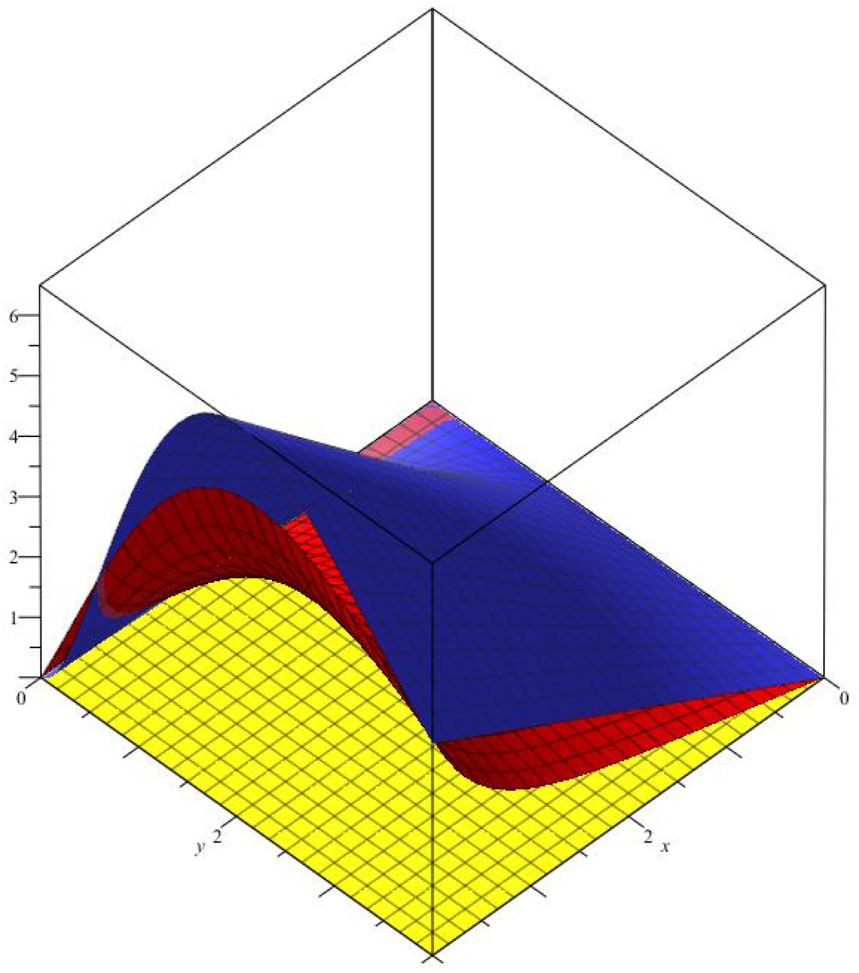
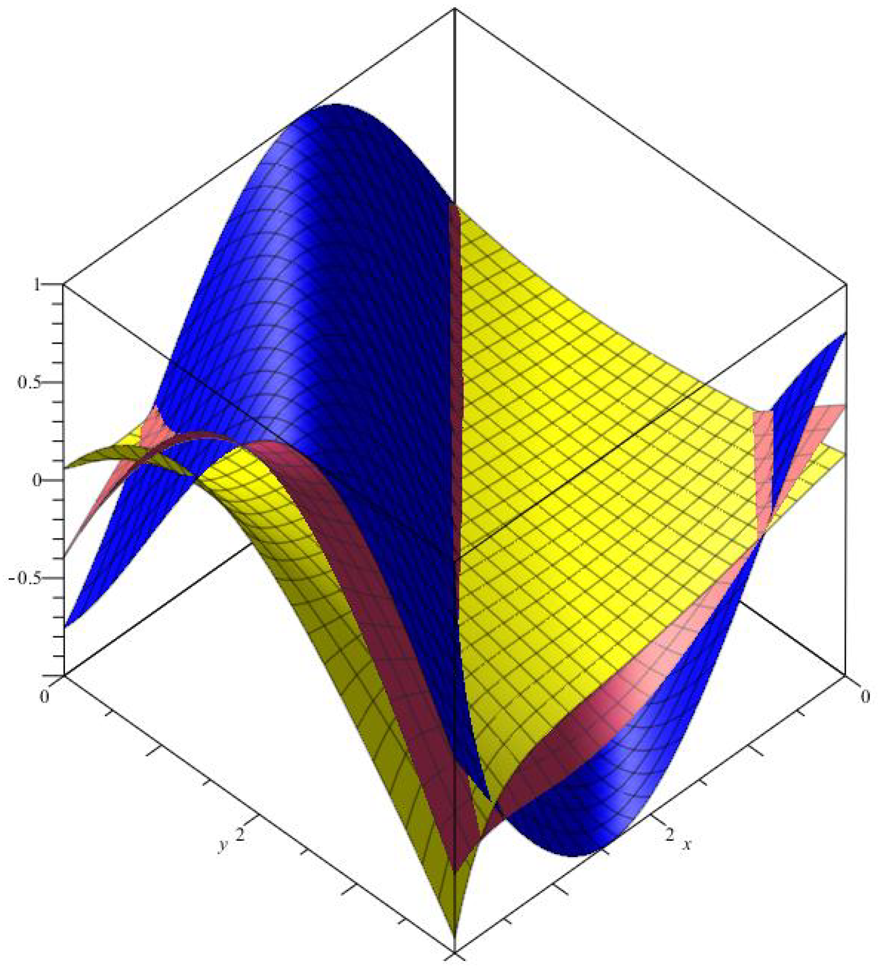
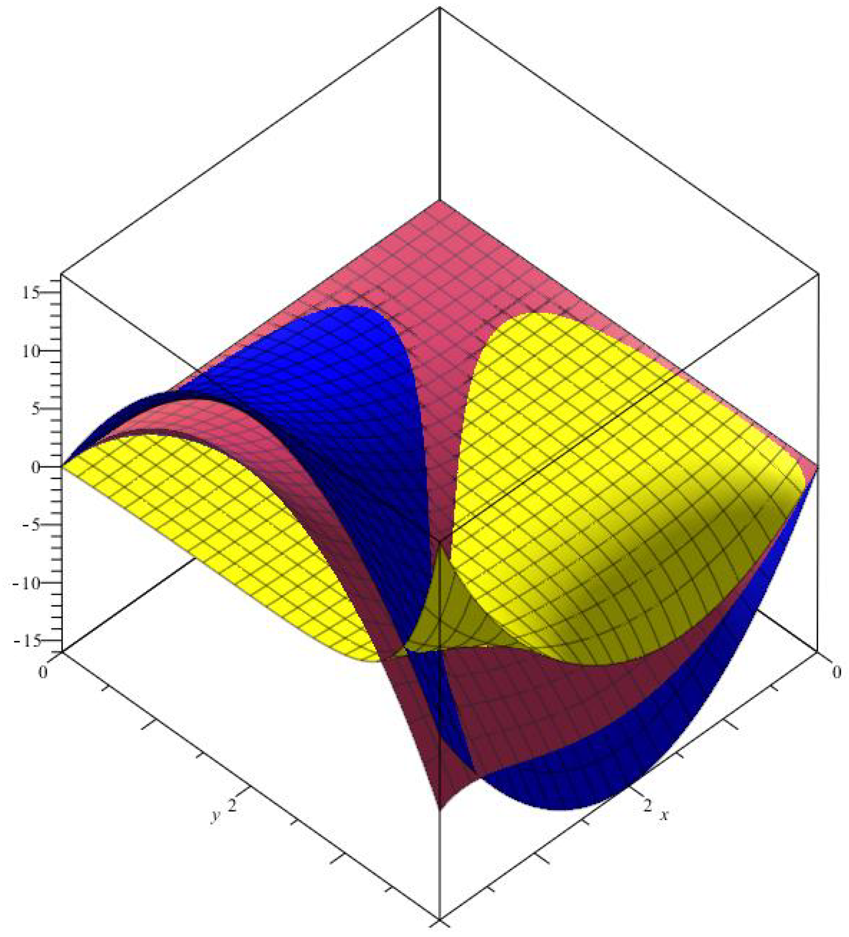
Figure 1. The comparison convergence of $C_{20,20}^{(0.999,0.9),(0.999,0.9)}(f;x,y)$(red), $C_{20,20}^{(0.90,0.86),(0.996,0.89)}(f;x,y)$(yellow) with ${\alpha }_n=ln\left(n\right)$, ${\beta }_m=\sqrt{m}$ and $f(x,y)=3x{y}^2{e}^{-y}$(blue)

Figure 1. The comparison convergence of $C_{20,20}^{(0.999,0.9),(0.999,0.9)}(f;x,y)$(red), $C_{20,20}^{(0.90,0.86),(0.996,0.89)}(f;x,y)$(yellow) with ${\alpha }_n=ln\left(n\right)$, ${\beta }_m=\sqrt{m}$ and $f(x,y)=3x{y}^2{e}^{-y}$(blue)

Figure 2. The comparison convergence of $C_{20,20}^{(0.999,0.9),(0.99,0.9)}(f;x,y)$(red), $C_{20,20}^{(0.990,0.86),(0.996,0.89)}(f;x,y)$(yellow) with ${\alpha }_n=ln\left(n\right)$, ${\beta }_m=\sqrt{m}$ and $f(x,y)=sin(x-y)$(blue).

Figure 2. The comparison convergence of $C_{20,20}^{(0.999,0.9),(0.99,0.9)}(f;x,y)$(red), $C_{20,20}^{(0.990,0.86),(0.996,0.89)}(f;x,y)$(yellow) with ${\alpha }_n=ln\left(n\right)$, ${\beta }_m=\sqrt{m}$ and $f(x,y)=sin(x-y)$(blue).

Figure 3. The comparison convergence of $C_{20,20}^{(0.99,0.9),(0.999,0.96)}(f;x,y)$(red), $C_{20,20}^{(0.99,0.9),(0.990,0.90)}(f;x,y)$(yellow) with ${\alpha }_n=ln\left(n\right)$, ${\beta }_m=ln\left(m\right)$ and $f(x,y)=x^{2}y-x{y}^2)$(blue).

Figure 3. The comparison convergence of $C_{20,20}^{(0.99,0.9),(0.999,0.96)}(f;x,y)$(red), $C_{20,20}^{(0.99,0.9),(0.990,0.90)}(f;x,y)$(yellow) with ${\alpha }_n=ln\left(n\right)$, ${\beta }_m=ln\left(m\right)$ and $f(x,y)=x^{2}y-x{y}^2)$(blue).

Theorem 6. 

Let $f\in C\left(I_{ab}\right)$, then we have

$$\begin{array}{c}\hfill {∥C_{n,m}^{(p_1,q_1),(p_2,q_2)}\left(f;x,y\right)-f(x,y)∥}_{C\left(I_{ab}\right)}\le 2M\left(f;{\delta }_{n,m}(x,y)/2\right),\end{array}$$

where

$$\begin{array}{c}\hfill {\delta }_{n,m}(x,y)={\displaystyle \frac{1}{2}}max\left({\displaystyle \frac{a{\alpha }_n{p}_1^{n-1}}{{\left[n\right]}_{p_1,q_1}}},{\displaystyle \frac{b{\beta }_m{p}_2^{m-1}}{{\left[m\right]}_{p_2,q_2}}}\right).\end{array}$$

Proof. 

Let $g\in C^2\left(I_{ab}\right)$. By the Taylor’s formula, we get

$$\begin{array}{ccc}\hfill g(s_1,s_2)-g(x,y)& =& g(s_1,y)-g(x,y)+g(s_1,s_2)-g(s_1,y)\hfill \\ & =& {\displaystyle \frac{\partial g(x,y)}{\partial x}}(s_1-x)+{\int }_x^{s_1}(s_1-u){\displaystyle \frac{{\partial }^{2}g(u,y)}{\partial u^2}}du\hfill \\ & & +{\displaystyle \frac{\partial g(x,y)}{\partial x}}(s_2-y)+{\int }_y^{s_2}(s_2-v){\displaystyle \frac{{\partial }^{2}g(x,v)}{\partial v^2}}dv\hfill \\ & =& {\displaystyle \frac{\partial g(x,y)}{\partial x}}(s_1-x)+{\int }_0^{s_1-x}(s_1-x-u){\displaystyle \frac{{\partial }^{2}g(u,y)}{\partial u^2}}du\hfill \\ & & +{\displaystyle \frac{\partial g(x,y)}{\partial x}}(s_2-y)+{\int }_0^{s_2-y}(s_2-y-v){\displaystyle \frac{{\partial }^{2}g(x,v)}{\partial v^2}}dv\hfill \end{array}$$

Applying $C_{n,m}^{(p_1,q_1),(p_2,q_2)}$ to the both sides of the above equation, we obtain

$$\begin{array}{ccc}\hfill \left|C_{n,m}^{(p_1,q_1),(p_2,q_2)}\left(g;x,y\right)-g(x,y)\right|& \le & \left|{\displaystyle \frac{\partial g(x,y)}{\partial x}}\right|\left|C_{n,m}^{(p_1,q_1),(p_2,q_2)}\left((s_1-x);x,y\right)\right|\hfill \\ & & +\left|C_{n,m}^{(p_1,q_1),(p_2,q_2)}\left({\int }_0^{s_1-x}(s_1-x-u){\displaystyle \frac{{\partial }^{2}g(u,y)}{\partial u^2}}du;x,y\right)\right|\hfill \\ & & +\left|{\displaystyle \frac{\partial g(x,y)}{\partial y}}\right|\left|C_{n,m}^{(p_1,q_1),(p_2,q_2)}\left((s_2-y);x,y\right)\right|\hfill \\ & & +\left|C_{n,m}^{(p_1,q_1),(p_2,q_2)}\left({\int }_0^{s_2-y}(s_2-y-v){\displaystyle \frac{{\partial }^{2}g(v,x)}{\partial v^2}}dv;x,y\right)\right|\hfill \end{array}$$

As $C_{n,m}^{(p_1,q_1),(p_2,q_2)}\left((s_1-x);x,y\right)=0$ and $C_{n,m}^{(p_1,q_1),(p_2,q_2)}\left((s_2-y);x,y\right)=0$, one can write following

$$\begin{array}{ccc}\hfill {∥C_{n,m}^{(p_1,q_1),(p_2,q_2)}\left(f;x,y\right)-f(x,y)∥}_{C\left(I_{ab}\right)}& \le & {\displaystyle \frac{1}{2}}{∥{\displaystyle \frac{\partial g(x,y)}{\partial x}}∥}_{C\left(I_{ab}\right)}\left|C_{n,m}^{(p_1,q_1),(p_2,q_2)}\left({(s_1-x)}^2;x,y\right)\right|\hfill \\ & & +{\displaystyle \frac{1}{2}}{∥{\displaystyle \frac{\partial g(x,y)}{\partial y}}∥}_{C\left(I_{ab}\right)}\left|C_{n,m}^{(p_1,q_1),(p_2,q_2)}\left({(s_2-y)}^2;x,y\right)\right|.\hfill \end{array}$$

By (5), (6), we deduce,

$$\begin{array}{ccc}\hfill {∥C_{n,m}^{(p_1,q_1),(p_2,q_2)}\left(f;x,y\right)-f(x,y)∥}_{C\left(I_{ab}\right)}& \le & {\displaystyle \frac{1}{2}}max\left({\displaystyle \frac{-p_1^{n-1}{x}^2}{{\left[n\right]}_{p_1,q_1}}}+{\displaystyle \frac{x{p}_1^{n-1}{\alpha }_n}{{\left[n\right]}_{p_1,q_1}}},{\displaystyle \frac{-p_2^{m-1}{y}^2}{{\left[m\right]}_{p_2,q_2}}}+{\displaystyle \frac{y{p}_2^{m-1}{\beta }_m}{{\left[m\right]}_{p_2,q_2}}}\right)\hfill \\ & & \times \left[{∥{\displaystyle \frac{\partial g(x,y)}{\partial x}}∥}_{C\left(I_{ab}\right)}+{∥{\displaystyle \frac{\partial g(x,y)}{\partial x}}∥}_{C\left(I_{ab}\right)}\right]\hfill \\ & \le & {\Vert g\Vert }_{C\left(I_{ab}\right)}{\delta }_{n,m}.\hfill \end{array}$$

(10)

By the linearity $C_{n,m}^{(p_1,q_1),(p_2,q_2)}$, we obtain

$$\begin{array}{ccc}\hfill {∥C_{n,m}^{(p_1,q_1),(p_2,q_2)}\left(f;x,y\right)-f(x,y)∥}_{C\left(I_{ab}\right)}& \le & {∥C_{n,m}^{(p_1,q_1),(p_2,q_2)}f-C_{n,m}^{(p_1,q_1),(p_2,q_2)}g∥}_{C\left(I_{ab}\right)}\hfill \\ & & +{∥C_{n,m}^{(p_1,q_1),(p_2,q_2)}g-g∥}_{C\left(I_{ab}\right)}+{∥f-g∥}_{C\left(I_{ab}\right)}.\hfill \end{array}$$

(11)

By (10) and (11), one can see that

$$\begin{array}{c}\hfill {∥C_{n,m}^{(p_1,q_1),(p_2,q_2)}\left(f;x,y\right)-f(x,y)∥}_{C\left(I_{ab}\right)}\le 2M\left(f;{\delta }_{n,m}(x,y)/2\right).\end{array}$$

This step completes the proof. □

First, we need the auxiliary result contained in the following lemma.

Lemma 3. 

Let $0<q_n<p_n\le 1$ be sequences such that $p_n,q_n⟶1$ and $p_n^n⟶a_1$ as $n⟶\infty$. Then, we have the following limits:

(i)

${lim}_{n\to \infty }{\displaystyle \frac{{\left[n\right]}_{p_n,q_n}}{{\alpha }_n}}{C}_{n,n}^{(p_n,q_n)}({(t-x)}^2;x)=a_{1}x$

(ii)

${lim}_{n\to \infty }{\displaystyle \frac{{\left[n\right]}_{p_n,q_n}^2}{{\alpha }_n^2}}{C}_{n,n}^{(p_n,q_n)}({(t-x)}^4;x)=3a_1{x}^2$.

Proof. (i) Using Lemma 1, we have

$$\begin{array}{c}\hfill C_{n,n}^{(p_n,q_n)}({(t-x)}^2;x)={\displaystyle \frac{-p_n^{n-1}{x}^2}{{\left[n\right]}_{p_n,q_n}}}+{\displaystyle \frac{x{p}_n^{n-1}{\alpha }_n}{{\left[n\right]}_{p_n,q_n}}}\end{array}$$

(12)

Then, we get

$$\begin{array}{c}\hfill {\displaystyle \frac{{\left[n\right]}_{p_n,q_n}}{{\alpha }_n}}{C}_{n,n}^{(p_n,q_n)}({(t-x)}^2;x)={\displaystyle \frac{-p_n^{n-1}{x}^2}{{\alpha }_n}}+x{p}_n^{n-1}.\end{array}$$

Let us take the limit of both sides of the above equality as $n⟶\infty$, then we can write

$$\begin{array}{ccc}\hfill \underset{n\to \infty }{lim}{\displaystyle \frac{{\left[n\right]}_{p_n,q_n}}{{\alpha }_n}}\left\{C_{n,n}^{(p_n,q_n)}({(t-x)}^2,x)\right\}& =& \underset{n\to \infty }{lim}\left\{{\displaystyle \frac{-p_n^{n-1}{x}^2}{{\alpha }_n}}+x{p}_n^{n-1}\right\}\hfill \\ & =& a_{1}x.\hfill \end{array}$$

(ii) By Lemma 1 and by the linearity of the operators $C_{n,n}^{(p_n,q_n)}$, we have

$$\begin{array}{c}\hfill C_{n,n}^{(p_n,q_n)}({(t-x)}^4;x)=A_{1,n}{x}^4+A_{2,n}{x}^3+A_{3,n}{x}^2+A_{4,n}x\end{array}$$

(13)

where

$$\begin{array}{ccc}\hfill A_{1,n}& =& {\displaystyle \frac{p_n^{n-3}{\left[n\right]}_{p_n,q_n}^2(-p_n^2+2p_n{q}_n-q_n^2)+p_n^{n-5}{\left[n\right]}_{p_n,q_n}(-p_n^3+3p_n{q}_n^2+q_n^3)-p_n^{3n-6}(p_n^2+p_n^3+2p_n{q}_n^2+q_n^3)}{{\left[n\right]}_{p_n,q_n}^3}}\hfill \\ \hfill A_{2,n}& =& {\displaystyle \frac{p_n^{n-3}{\left[n\right]}_{p_n,q_n}^2(p_n^2-2p_n{q}_n+q_n^2)}{{\left[n\right]}_{p_n,q_n}^3}}{\alpha }_n\hfill \\ & & +{\displaystyle \frac{p^{2n-5}{\left[n\right]}_{p_n,q_n}(-q_n^3-4p_n{q}_n^2-3p_n^2{q}_n+2p_n^3)-p_n^{3n-6}(3p_n^3+3p_n{q}_n^2+5p_n^2{q}_n+q_n^3)}{{\left[n\right]}_{p_n,q_n}^3}}{\alpha }_n\hfill \\ \hfill A_{3,n}& =& {\displaystyle \frac{p_n^{2n-4}{\left[n\right]}_{p_n,q_n}(-p_n^2+3p_n{q}_n+q_n^2)-p_n^{3n-5}(3p_n^2+q_n^2+3p_n{q}_n)}{{\left[n\right]}_{p_n,q_n}^3}}{\alpha }_n^2\hfill \\ \hfill A_{4,n}& =& {\displaystyle \frac{p^{3n-3}{\alpha }_n^3}{{\left[n\right]}_{p_n,q_n}^3}},\hfill \end{array}$$

It is clear that

$$\begin{array}{c}\hfill \underset{n\to \infty }{lim}{\displaystyle \frac{{\left[n\right]}_{p_n,q_n}^2}{{\alpha }_n^2}}\left\{A_{4,n}x\right\}=0.\end{array}$$

(14)

Taking the limit of both sides of $A_{1,n}$, we get

$$\begin{array}{ccc}\hfill \underset{n\to \infty }{lim}{\displaystyle \frac{{\left[n\right]}_{p_n,q_n}^2}{{\alpha }_n^2}}\left\{A_{1,n}\right\}& =& \underset{n\to \infty }{lim}\left\{{\displaystyle \frac{-p_n^{n-3}{\left[n\right]}_{p_n,q_n}{(p_n-q_n)}^2}{{\alpha }_n^2}}+{\displaystyle \frac{p_n^{n-5}(-p_n^3+3p_n{q}_n^2+q_n^3)}{{\alpha }_n^2}}-{\displaystyle \frac{p_n^{3n-6}(p_n^2+p_n^3+2p_n{q}_n^2+q_n^3)}{{\left[n\right]}_{p_n,q_n}{\alpha }_n^2}}\right\}\hfill \\ & =& \underset{n\to \infty }{lim}\left\{{\displaystyle \frac{-p_n^{n-3}(p_n^n-q_n^n)(p_n-q_n)}{{\alpha }_n^2}}+{\displaystyle \frac{p^{n-5}(-p_n^3+3p_n{q}_n^2+q_n^3)}{{\alpha }_n^2}}-{\displaystyle \frac{p_n^{3n-6}(p_n^2+p_n^3+2p_n{q}_n^2+q_n^3)}{{\left[n\right]}_{p_n,q_n}{\alpha }_n^2}}\right\}\hfill \\ & =& 0.\hfill \end{array}$$

(15)

Similarly, we can show that;

$$\begin{array}{c}\hfill \underset{n\to \infty }{lim}{\displaystyle \frac{{\left[n\right]}_{p_n,q_n}^2}{{\alpha }_n^2}}\left\{A_{2,n}\right\}=0\mathrm{and}\underset{n\to \infty }{lim}{\displaystyle \frac{{\left[n\right]}_{p_n,q_n}^2}{{\alpha }_n^2}}\left\{A_{3,n}\right\}=3a_1{x}^2\end{array}$$

(16)

By combining (14)-(16), we reach the desired the result. □

Now, we ready present a Voronovskaja type theorem for $C_{n,n}^{(p_n,q_n)}(f;x,y)$.

Theorem 7. 

Let $f\in C^2\left(I_{ab}\right)$. Then, we have

$$\begin{array}{ccc}\hfill \underset{n\to \infty }{lim}{\left[n\right]}_{p_n,q_n}{C}_{n,n}^{(p_n,q_n)}(f;x,y)-f\left(x_{,}y\right))& =& {\displaystyle \frac{a_{1}x{f}_{x^2}^{\prime \prime }(x,y)}{2}}+{\displaystyle \frac{a_{1}y{f}_{y^2}^{\prime \prime }(x,y)}{2}}.\hfill \end{array}$$

Proof. 

Let $(x,y)\in I_{ab}$. Then, write Taylor’s formula of f as follows:

$$\begin{array}{ccc}\hfill f(s,t)& =& f(x,y)+f_x^{\prime }(s-x)+f_y^{\prime }(t-y)\hfill \\ & & +{\displaystyle \frac{1}{2}}\left\{f_x^{″}{(t-x)}^2+2f_{xy}^{\prime }(s-x)(t-y)+f_y^{″}{(t-y)}^2\right\}+\epsilon (s,t)\left({(s-x)}^2+{(t-y)}^2\right)\hfill \end{array}$$

(17)

where $(s,t)\in I_{ab}$ and $\epsilon (s,t)⟶0$ as $(s,t)⟶(x,y)$.

If we apply the operator $C_{n,n}^{(p_n,q_n)}(f;.)$ on (17), we obtain

$$\begin{array}{ccc}\hfill C_{n,n}^{(p_n,q_n)}(f;s,t)-f\left(x_{,}y\right)& =& f_x^{\prime }(x,y)C_{n,n}^{(p_n,q_n)}((s-x);x,y)+f_y^{\prime }(x,y)C_{n,n}^{(p_n,q_n)}((t-y);x,y)\hfill \\ & & +{\displaystyle \frac{1}{2}}\{f_{x^2}^{\prime \prime }{C}_{n,n}^{(p_n,q_n)}({(t-x_0)}^2;x,y)+2f_{xy}^{\prime }{C}_{n,n}^{(p_n,q_n)}((s-x)(t-y);x,y)\hfill \\ & & +f_{y^2}^{\prime \prime }{C}_{n,n}^{(p_n,q_n)}({(t-y)}^2;x,y)\}+C_{n,n}^{(p_n,q_n)}\left(\epsilon (s,t)\left({(s-x)}^2+{(t-y)}^2\right);x,y\right).\hfill \end{array}$$

Applying the limit of both sides of the above equality, we get $n⟶\infty$, □

$$\begin{array}{ccc}\hfill \underset{n\to \infty }{lim}{\left[n\right]}_{p_n,q_n}{C}_{n,n}^{(p_n,q_n)}(f;s,t)-f(x,y))& =& \underset{n\to \infty }{lim}{\left[n\right]}_{p_n,q_n}{\displaystyle \frac{1}{2}}\{f_{x^2}^{\prime \prime }{C}_{n,n}^{(p_n,q_n)}({(t-x)}^2;x,y)\hfill \\ & & +2f_{xy}^{\prime }{C}_{n,n}^{(p_n,q_n)}((s-x)(t-y);x,y)+f_{y^2}^{\prime \prime }{C}_{n,n}^{(p_n,q_n)}({(t-y)}^2;x,y)\}\hfill \\ & & +\underset{n\to \infty }{lim}{\left[n\right]}_{p_n,q_n}{C}_{n,n}^{(p_n,q_n)}\left(\epsilon (s,t)\left({(s-x)}^2+{(t-y)}^2\right);x,y\right).\hfill \end{array}$$

By Cauchy-Schwartz inequality, we can write the following

$$\begin{array}{ccc}\hfill C_{n,n}^{(p_n,q_n)}\left(\epsilon (s,t)\left({(s-x)}^2+{(t-y)}^2\right);x,y\right)& \le & \sqrt{{lim}_{n\to \infty }{C}_{n,n}^{(p_n,q_n)}\left({\epsilon }^2(s,t);x,y\right)}\hfill \\ & \times & \sqrt{2{lim}_{n\to \infty }{\left[n\right]}_{p_n,q_n}^2{C}_{n,n}^{(p_n,q_n)}\left(\epsilon (s,t)\left({(s-x)}^4+{(t-y)}^4\right);x,y\right)}.\hfill \end{array}$$

As ${lim}_{n\to \infty }{C}_{n,n}^{(p_n,q_n)}\left({\epsilon }^2(s,t);x,y\right)={\epsilon }^2(x,y)=0$ and from Lemma 3(ii)

${lim}_{n\to \infty }{\left[n\right]}_{p_n,q_n}^2{C}_{n,n}^{(p_n,q_n)}\left({(s-x)}^4+{(t-y)}^4);x,y\right)$ is finite, then we have

$$\begin{array}{c}\hfill \underset{n\to \infty }{lim}{\left[n\right]}_{p_n,q_n}^2{C}_{n,n}^{(p_n,q_n)}\left(\epsilon (s,t)\left({(s-x)}^4+{(t-y)}^4\right);x,y\right)=0.\end{array}$$

Hence, we deduce

$$\begin{array}{ccc}\hfill \underset{n\to \infty }{lim}{\left[n\right]}_{p_n,q_n}{C}_{n,n}^{(p_n,q_n)}(f;x,y)-f\left(x_{,}y\right))& =& {\displaystyle \frac{a_{1}x{f}_{x^2}^{″}(x,y)}{2}}+{\displaystyle \frac{a_{1}y{f}_{y^2}^{″}(x,y)}{2}}.\hfill \end{array}$$

This step completes the proof.

4. Weighted Approximation Properties of Two Variable Function

In this section, the convergence of the sequence of linear positive operator $C_{n,m}^{(p_1,q_1),(p_2,q_2)}$ to a functions of two variables which defined on weighted space and compute rate of convergence via weighted modulus continuity.

Let $\rho (x,y)=x^2+y^2+1$ and $B_{\rho }$ be the space of all functions f defined on the real axis provide with $\left|f(x,y)\right|\le M_f\rho (x,y),$ where $M_f$ is a positive constant depending only on f. Let $C_{\rho }$ be the subspace of $B_{\rho }$ of all continuous functions with the norm:

$${\Vert f\Vert }_{\rho }=\underset{\left(x,y\right)\in {\mathbb{R}}_{+}^2}{sup}{\displaystyle \frac{\left|f\right(x,y\left)\right|}{\rho \left(x,y\right)}}.$$

Let $C_{\rho }^0$ denote the subspace of all functions $f\in C_{\rho }$ such that ${lim}_{x\to \infty }{\displaystyle \frac{f(x,y)}{\rho \left(x,y\right)}}$ exists finitely. For all $f\in C_{\rho }^0,$ the weighted modulus of continuity is defined by

$${\Omega }_f(f;{\delta }_1,{\delta }_2)=\underset{\left(x,y\right)\in {\mathbb{R}}_{+}^2}{sup}\underset{\left|h_1\right|\le {\delta }_1,\left|h_2\right|\le {\delta }_2}{sup}{\displaystyle \frac{\left|f(x+h_1,y+h_2)-f(x,y)\right|}{\rho (x,y)\rho (h_1,h_2)}}.$$

(18)

Lemma 4. 

The operators $C_{n,m}^{(p_1,q_1),(p_2,q_2)}$ defined (2) act from $C_{\rho }\left({\mathbb{R}}_{+}^2\right)$ to $B_{\rho }\left({\mathbb{R}}_{+}^2\right)$ if and only if the inequality

$$\begin{array}{c}\hfill \Vert C_{n,m}^{(p_1,q_1),(p_2,q_2)}{(\rho ;x,y)\Vert }_{x^2}\le c.\end{array}$$

holds for some positive constant c.

Theorem 8. 

Let $C_{n,m}^{(p_1,q_1),(p_2,q_2)}$ be sequence of linear positive operators defined (2), then for each $f\in C_{\rho }^0$ and for all $(x;y)\in I_{{\alpha }_n{\beta }_m}$, we have

$$\begin{array}{c}\hfill \underset{n\to \infty }{lim}{\Vert C_{n,m}^{(p_1,q_1),(p_2,q_2)}(f;x,y)-f(x,y)\Vert }_{\rho }=0.\end{array}$$

Proof. 

From Lemma 2, we obtain

$$\begin{array}{ccc}\hfill \Vert C_{n,m}^{(p_1,q_1),(p_2,q_2)}\left(1;x,y\right){-1\Vert }_{\rho }& =& 0,\hfill \\ \hfill \Vert C_{n,m}^{(p_1,q_1),(p_2,q_2)}\left(s;x,y\right){-x\Vert }_{\rho }& =& 0\hfill \\ \hfill \Vert C_{n,m}^{(p_1,q_1),(p_2,q_2)}\left(t;x,y\right){-y\Vert }_{\rho }& =& 0.\hfill \end{array}$$

Again by Lemma 2, we can write following

$$\begin{array}{ccc}& & \Vert C_{n,m}^{(p_1,q_1),(p_2,q_2)}(s^2+t^2;x,y)-(x^2+y^2){\Vert }_{\rho }\hfill \\ & =& \underset{(x,y)\in {\mathbb{R}}_{+}^2}{sup}\left\{{\displaystyle \frac{p_1^{n-1}{\alpha }_{n}x}{{\left[n\right]}_{p_1,q_1}(x^2+y^2+1)}}+{\displaystyle \frac{p_1^{n-1}{x}^2}{{\left[n\right]}_{p_1,q_1}(x^2+y^2+1)}}+{\displaystyle \frac{p_2^{m-1}{\beta }_{m}y}{{\left[m\right]}_{p_2,q_2}(x^2+y^2+1)}}+{\displaystyle \frac{p_2^{m-1}{y}^2}{{\left[m\right]}_{p_2,q_2}(x^2+y^2+1)}}\right\}\hfill \\ & \le & {\displaystyle \frac{p_1^{n-1}{\alpha }_n}{{\left[n\right]}_{p_1,q_1}}}+{\displaystyle \frac{p_1^{n-1}}{{\left[n\right]}_{p_1,q_1}}}+{\displaystyle \frac{p_2^{m-1}{\beta }_m}{{\left[m\right]}_{p_2,q_2}}}+{\displaystyle \frac{p_2^{m-1}}{{\left[m\right]}_{p_2,q_2}}}\hfill \end{array}$$

Taking the limit of both sides of above inequality as $n,m⟶\infty$ with by (3) and (4), we get

$$\begin{array}{c}\hfill \underset{m,n\to \infty }{lim}{\Vert C_{n,m}^{(p_1,q_1),(p_2,q_2)}(s^2+t^2;x,y)-(x^2+y^2)\Vert }_{\rho }=0.\end{array}$$

Applying weighted Korovkin theorem for two variable which presented by Gadzhiev [4,5], we get desired the results. □

For estimate rate of convergence we need the following lemma.

Lemma 5. 

For all $(x;y)\in I_{{\alpha }_n{\beta }_m}$, by (5), (6) and (13), one can write the following

$$\begin{array}{ccc}\hfill C_{n,m}^{(p_1,q_1),(p_2,q_2)}\left({\left(t-x\right)}^2;x,y\right)& =& O\left({\displaystyle \frac{{\alpha }_n{p}_1^{n-1}}{{\left[n\right]}_{p_1,q_1}}}\right)\left(x^2+x\right),\hfill \end{array}$$

(19)

$$\begin{array}{ccc}\hfill C_{n,m}^{(p_1,q_1),(p_2,q_2)}\left({\left(t-x\right)}^4;x,y\right)& =& O\left({\displaystyle \frac{{\alpha }_n{p}_1^{n-1}}{{\left[n\right]}_{p_1,q_1}}}\right)\left(x^4+x^3+x^2+x\right)\hfill \end{array}$$

(20)

and

$$\begin{array}{ccc}\hfill C_{n,m}^{(p_1,q_1),(p_2,q_2)}\left({\left(s-y\right)}^2;x,y\right)& =& O\left({\displaystyle \frac{{\beta }_m{p}_2^{m-1}}{{\left[m\right]}_{p_2,q_2}}}\right)\left(y^2+y+1\right),\hfill \end{array}$$

(21)

$$\begin{array}{ccc}\hfill C_{n,m}^{(p_1,q_1),(p_2,q_2)}\left({\left(s-y\right)}^4;x,y\right)& =& O\left({\displaystyle \frac{{\beta }_m{p}_2^{m-1}}{{\left[m\right]}_{p_2,q_2}}}\right)\left(y^4+y^3+y^2+y+1\right).\hfill \end{array}$$

(22)

Now, compute rate of convergence the operator $C_{n,m}^{(p_1,q_1),(p_2,q_2)}$ in weighted spaces .

Theorem 9. 

If $f\in C_{\rho }^0,$ then we have

$$\underset{\left(x,y\right)\in {\mathbb{R}}_{+}^2}{sup}{\displaystyle \frac{\left|C_{n,m}^{(p_1,q_1),(p_2,q_2)}(f;x,y)-f(x,y)\right|}{\rho {\left(x,y\right)}^3}}\le {\mathcal{C}}_2{\omega }_{\rho }(f;{\delta }_n,{\delta }_m)$$

, where ${\mathcal{C}}_2$ is a constant independent of $n,m$ and ${\delta }_n={\displaystyle \frac{p_1^{n-1}{\alpha }_n}{{\left[n\right]}_{p_1,q_1}}}$, ${\delta }_n={\displaystyle \frac{p_2^{m-1}{\beta }_m}{{\left[m\right]}_{p_2,q_2}}}$ .

Proof. 

Taking into account the following inequality given in [9], we deduce

$$\left|f\left(t,s\right)-f\left(x,y\right)\right|\le 8\left(1+x^2+y^2\right){\omega }_{\rho }(f;{\delta }_n,{\delta }_m)$$

$$\times \left(1+{\displaystyle \frac{\left|t-x\right|}{{\delta }_n}}\right)\left(1+{\displaystyle \frac{\left|s-y\right|}{{\delta }_m}}\right)\left(1+{\left(t-x\right)}^2\right)\left(1+{\left(s-y\right)}^2\right).$$

Applying $C_{n,m}^{(p_1,q_1),(p_2,q_2)}$ both side above inequality and using Cauchy-Schwarz inequality, one can write following

$$\left|C_{n,m}^{(p_1,q_1),(p_2,q_2)}(f;x,y)-f(x,y)\right|\le 8\left(1+x^2+y^2\right){\omega }_{\rho }(f;{\delta }_n,{\delta }_m)$$

$$\times \left[1+C_{n,m}^{(p_1,q_1),(p_2,q_2)}\left({\left(t-x\right)}^2;x,y\right)+{\displaystyle \frac{1}{{\delta }_n}}\sqrt{C_{n,m}^{(p_1,q_1),(p_2,q_2)}\left({\left(t-x\right)}^2;x,y\right)}\right.$$

$$\left.{\displaystyle \frac{1}{{\delta }_n}}\sqrt{C_{n,m}^{(p_1,q_1),(p_2,q_2)}\left({\left(t-x\right)}^2;x,y\right)C_{n,m}^{(p_1,q_1),(p_2,q_2)}\left({\left(t-x\right)}^4;x,y\right)}\right]$$

$$\times \left[1+C_{n,m}^{(p_1,q_1),(p_2,q_2)}\left({\left(s-y\right)}^2;x,y,a\right)+{\displaystyle \frac{1}{{\delta }_m}}\sqrt{C_{n,m}^{(p_1,q_1),(p_2,q_2)}\left({\left(s-y\right)}^2;x,y\right)}\right.$$

$$\times \left.{\displaystyle \frac{1}{{\delta }_m}}\sqrt{C_{n,m}^{(p_1,q_1),(p_2,q_2)}\left({\left(s-y\right)}^2;x,y\right)C_{n,m}^{(p_1,q_1),(p_2,q_2)}\left({\left(s-y\right)}^4;x,y\right)}\right].$$

By (19)-(22), we obtain

$$\left|C_{n,m}^{(p_1,q_1),(p_2,q_2)}(f;x,y)-f(x,y)\right|\le 8\left(1+x^2+y^2\right){\omega }_{\rho }(f;{\delta }_n,{\delta }_m)$$

$$\times \left[1+O\left({\displaystyle \frac{p_1^{n-1}{\alpha }_n}{{\left[n\right]}_{p_1,q_1}}}\right)\left(x^2+x\right)+{\displaystyle \frac{1}{{\delta }_n}}\sqrt{O\left({\displaystyle \frac{p_1^{n-1}{\alpha }_n}{{\left[n\right]}_{p_1,q_1}}}\right)\left(x^2+x\right)}\right.$$

$$\left.+{\displaystyle \frac{1}{{\delta }_n}}\sqrt{O\left({\displaystyle \frac{p_1^{n-1}{\alpha }_n}{{\left[n\right]}_{p_1,q_1}}}\right)\left(x^2+x\right)\left(x^4+x^3+x^2+x\right)}\right]$$

$$\times \left[1+{\displaystyle \frac{p_2^{m-1}{\beta }_m}{{\left[m\right]}_{p_2,q_2}}}\left(y^2+y\right)+{\displaystyle \frac{p_2^{m-1}{\beta }_m}{{\left[m\right]}_{p_2,q_2}}}\sqrt{{\displaystyle \frac{p_2^{m-1}{\beta }_m}{{\left[m\right]}_{p_2,q_2}}}}\right.$$

$$\left.+{\displaystyle \frac{1}{{\delta }_m}}\sqrt{{\displaystyle \frac{p_2^{m-1}{\beta }_m}{{\left[m\right]}_{p_2,q_2}}}\left(y^2+y\right){\displaystyle \frac{p_2^{m-1}{\beta }_m}{{\left[m\right]}_{p_2,q_2}}}\left(y^4+y^3+y^2+y\right)}\right].$$

Taking ${\delta }_n={\left({\displaystyle \frac{p_1^{n-1}{\alpha }_n}{{\left[n\right]}_{p_1,q_1}}}\right)}^{1/2},{\delta }_m={\left({\displaystyle \frac{p_2^{m-1}{\beta }_m}{{\left[m\right]}_{p_2,q_2}}}\right)}^{1/2}$, one write the following:

$$\left|C_{n,m}^{(p_1,q_1),(p_2,q_2)}(f;x,y)-f(x,y)\right|\le {\mathcal{C}}_2\left(1+x^2+y^2\right){\omega }_{\rho }(f;{\delta }_n,{\delta }_m)$$

$$\times \left[1+{\delta }_n^2\left(x^2+x\right)+\sqrt{x^2+x}+\sqrt{\left(x^2+x\right)\left(x^4+x^3+x^2+x\right)}\right]$$

$$\times \left[1+{\delta }_m^2\left(y^2+y\right)+\sqrt{\left(y^2+y\right)}+\sqrt{\left(y^2+y\right)\left(y^4+y^3+y^2+y\right)}\right],$$

where ${\mathcal{C}}_2$ is a constant independent of $n,m.$ Since ${\delta }_n^2<1,{\delta }_m^2<1,$ for sufficiently large $n,m,$ we get

$$\underset{\left(x,y\right)\in {\mathbb{R}}_{+}^2}{sup}{\displaystyle \frac{\left|C_{n,m}^{(p_1,q_1),(p_2,q_2)}(f;x,y)-f(x,y)\right|}{{\left(1+x^2+y^2\right)}^3}}\le {\mathcal{C}}_2{\omega }_{\rho }\left(f;\sqrt{{\displaystyle \frac{p_1^{n-1}{\alpha }_n}{{\left[n\right]}_{p_1,q_1}}}},\sqrt{{\displaystyle \frac{p_2^{m-1}{\beta }_m}{{\left[m\right]}_{p_2,q_2}}}}\right).$$

This step completes the proof. □

References

- A. Karaisa, Approximation by Durrmeyer type Jakimoski–Leviatan operators, Math Methods Appl Sci In Press(2015), 1–12. [CrossRef]
- Karaisa and F.Karakoc, Stancu type generalization of Dunkl analogue of Szàsz operators, Adv Appl, 1–14. [CrossRef]
- A. Karaisa, DT. Tollu and Y. Asar, Stancu type generalization of q-Favard-Szàsz operators, Appl Math Comput.(2015), 264: 249–257. [CrossRef]
- A D. Gadjiev, Linear positive operators in weighted space of functions of several variables, Izvestiya Acad of Sciences of Azerbaijan(1980), 1: 32-37.
- AD. Gadjiev, H. Hacýsalihoglu, On convergence of the sequences of linear positive operators, Ph. D. thesis, Ankara University, 1995, in Turkish.
- A. Lupaş, q-analogue of the Bernstein operator, Seminar on Numerical and Statistical Calculus, University of Cluj-Napoca(1987), 9: 85-92.
- AM. Acu and CV. Muraru, Approximation Properties of bivariate extension of q- Bernstein-Schurer-Kantorovich operators, Result Math.(2015), 67: 265–279. [CrossRef]
- A. Aral, V. Gupta and RP. Agarwal, Applications of q- calculus in operator theory, Berlin: Springer, 2013. [CrossRef]
- C. Atakut and N. Ispir, Approximation by modified Szász-Mirakjan operators on weighted spaces, Proc Indian Acad Sci Math.(2002), 112: 571-578. [CrossRef]
- D. Barbosu, Some Generalized Bivariate Bernstein Operators, Mathematical Notes Miskolc.(2000), 1: 3–10. [CrossRef]
- GA. Anastassiou and SG. Gal, Approximation theory: moduli of continuity and global smoothness preservation, Birkha¨user: Boston, 2000.
- H. Karsli, A Voronovskaya type theory for the second derivative of the Bernstein-Chlodovsky polynomials, Proc Est Acad Sci.(2012),61: 9–19. [CrossRef]
- I. Büyükyazıcı, On the approximation properties of two-dimensional q-Bernstein-Chlodowsky polynomials, Math Commun.(2009), 14: 255–269.
- I. Büyükyazıcı and H. Sharma Approximation properties of two-dimensional q-Bernstein–Chlodowsky–Durrmeyer operators, Numer Funct Anal Optim.(2012), 33:1351–1371. [CrossRef]
- I. Büyükyazıcı, Approximation by Stancu–Chlodowsky polynomials, Comput Math Appl., 2010; 59: 274–282. [CrossRef]
- KJ. Ansari and A. Karaisa, Chlodovsky type generalization of Bernstein operators based on (p,q) integer, under the cominication.
- M. Mursaleen, MD. Nasiuzzaman and A. Nurgali, Some approximation results on Bernstein–Schurer operators defined by (p,q)-integers, Jour Ineq Appl.(2015),249: 1–15. [CrossRef]
- M. Mursaleen, KJ. Ansari and A. Khan, Some approximation results by (p,q)-analogue of Bernstein–Stancu operators, Appl Math Comput.(2015),64: 392–402. [CrossRef]
- M. Mursaleen, MD. Nasiruzzaman, A. Khan and KJ. Ansari, Some approximation results on Bleimann-Butzer–Hahn operators defined by (p,q)-integers, 2015. [CrossRef]
- M. Mursaleen, KJ. Ansari and A. Khan, On (p,q)-analogue of Bernstein operators, Appl Math Comput.(2015). [CrossRef]
- M. Mursaleen, KJ. Ansari and A. Khan, Erratum to on (p,q)- analogue of Bernstein Operators, [Appl. Math. Comput. 266 (2015) 874-882] Appl. Math. Comput.(2016); 278: 70-71. [CrossRef]
- PL. Butzer and H. Berens, Semi-groups of operators and approximation, Springer, New York, 1967.
- PL. Butzer and H.Karsli, Voronovskaya-type theorems for derivatives of the Bernstein-Chlodovsky polynomials and the Szá sz–Mirakyan operator, Comment Math.(2009), 49: 33–58.
- PN. Agrawal and N. Ispir, Degree of Approximation for Bivariate Chlodowsky–Szász-Charlier Type Operator, Results Math.(2015). [CrossRef]
- Sadjang, On the fundamental theorem of (p,q)-calculus and some (p,q)-Taylor formulas, 2015; [math.QA]. [CrossRef]
- T. Acar, A. Aral and SA. Mohiuddine, Approximation by bivariate (p,q)-Bernstein–Kantorovich operator(2016), [math.CA]. [CrossRef]
- V. Gupta, (p,q)-Szàsz-Mirakyan-Baskakov operators, Complex Anal Oper Theory(2015), 1–9. [CrossRef]
- V. Sahai and S. Yadav Representations of two parameter quantum algebras and p,q-special functions, J Math Anal Appl.(2007), 335: 268-279. [CrossRef]
- VJ. Volkov, On the convergence of linear positive operators in the space of continuous functions of two variables, (Russian). Doklakad Nauk SSSR, (1957)115: 17-19.
Disclaimer/Publisher’s Note: The statements, opinions and data contained in all publications are solely those of the individual author(s) and contributor(s) and not of MDPI and/or the editor(s). MDPI and/or the editor(s) disclaim responsibility for any injury to people or property resulting from any ideas, methods, instructions or products referred to in the content. |
© 2024 by the authors. Licensee MDPI, Basel, Switzerland. This article is an open access article distributed under the terms and conditions of the Creative Commons Attribution (CC BY) license (http://creativecommons.org/licenses/by/4.0/).
Copyright: This open access article is published under a Creative Commons CC BY 4.0 license, which permit the free download, distribution, and reuse, provided that the author and preprint are cited in any reuse.