
Submitted:
09 October 2024
Posted:
11 October 2024
Read the latest preprint version here
Abstract
A new compounded distribution called the Topp-Leone-Lomax Poisson
is developed. The statistical properties of this model are derived. The
model parameters are estimated via the maximum likelihood technique.
The performance of the estimation techniques was assessed by means
of simulation studies. The new model was exposed to three data sets
and compared to other models within the same class and the evidence
supports the importance of the new model in data modelling.
Keywords:
Topp-Leone Lomax Distribution
; Power Series Distribution
; Maximum Likelihood Estimation
; Poisson Distribution
1. Introduction
Over the past two centuries, statistical distributions gained appreciation from many researchers as a means of describing data. A number of distributions were developed and these include the exponential distribution which was a very important lifetime distribution. This distribution was good in modelling lifetime data with constant failure rate. However, the distribution could not accommodate other failure rates that include decreasing, increasing and non-monotone. Lomax developed the shifted Pareto (Pareto II) or Lomax distribution [9] which is a mixture of the exponential and gamma distributions. This distribution applies to data with decreasing failure rate and has heavier tails compared to the Weibull [19] and gamma distributions. Statisticians came with solutions to address the short comings of classical distributions. These solutions include transformation of the classical distribution for example the T-X transformation by Alzaatreh et al. [4], gamma transformations by Zografos and Balakrishnan [20], Ristiç and Balakrishnan [15], and Torabi and Montazari [18], half logistic transformation by Cordeiro et al. [7], to mention a few. The other techniques for generalizing classical distribution includes exponentiation, power transformation, competing risks, and compounding methods.
Some generalizations of the Lomax distribution include the exponentiated Lomax (Exp-Lx) by Abdul-Moniem and Abdel-Hammed [2], exponential Lomax (E-Lx) by Bassiouny et al. [5], and the Weibull-Lomax (W-Lx) by Tahir et al. [17]. Oguntunde et al. [13] developed the Topp-Leone Lomax (TL-Lx) distribution using the generalization by Al-Shomrani et al. [3]. The TL-Lx distribution is a has a pdf that is skewed to the right. The TL-Lx distribution has cumulative distribution function (cdf) and probability density function (pdf) given by
and
respectively, for Other generalizations that involves the Topp-Leone generalization include the Topp-Leone odd exponential half logistic-G family of distributions by Chipepa and Oluyede [6], The Topp-Leone-Harris-G family of distributions with applications by Oluyede et al. [12], and the Topp-Leone odd Burr III-G family of distributions by Moakofi et al. [11].
This research generalizes the TL-LxP distribution by compounding it with the power series distribution. Power series distributions includes the Poisson, logarithmic, binomial, and geometric distributions as stated by Johnson et al. [8]. The Poisson distribution is considered as a special case from the power series distributions. Given a discrete random variable, say, M, having a power series distribution with probability mass function (pmf)
where is finite, and a sequence of positive real numbers. Taking the cumulative distribution function (cdf) and probability density function (pdf) of are defined by
and
where is the survival function given by .
2. The Model
In this paper, the TL-Lx distribution by Oguntunde et al. [13] is compounded with the Poisson power series distribution to produce a new model called the Topp-Leone-Lomax Poisson (TL-LxP) distribution. The pdf and the cdf of the TL-LxP distribution is given by
and
for The corresponding hazard rate function is given by
The pdf of the TL-LxP takes reverse-J shape, right or left-skewed shapes as shown in Figure 1.
3. Some Statistical Properties
We present in this section quantile function, moments, moment generation function, and Rényi Entropy.
3.1. Quantile Function
The quantile function is defined by That is
which simplifies to
3.2. Moments and Moment Generating Function
The raw moment () of the TL-LxP distribution is given by
with defined in Equation (7). Using the generalized binomial series expansion we have
Let implying and we get
Thus,
which is a beta function over a half line. Therefore, the moment is given by
This result is important in determining the moments and measures of central tendency and dispersion (standard deviation (SD), coefficient of variation (CV), coefficient of skewness (CS), and coefficient of kurtosis (CK)). Table 2 presents the first five moments and the measures of dispersion for selected parameter values ().
The moment generating function of the TL-LxP is given by
3.3. Distribution of Order Statistics
The pdf of the order statistics is given by
which is a linear combination of exponentiated TL-Lx distribution.
3.4. Rényi Entropy
The two commonly used measures of uncertainty are Shannon [16] and Rényi [14] entropies. Rényi entropy is a generalization of the Shannon entropy, hence, we will derive only the Rényi entropy in this paper. Rényi entropy for the TL-LxP distribution is derived as follows:
Now
Let ⇒⇒ When and when Note
Hence,
Therefore, we define Rényi entropy of the TL-LxP distribution by
4. Estimation
If with the parameter vector . The total log-likelihood from a random sample of size n is given by
The elements of the score vector are given below
. and
5. Simulations
To evaluate the consistency of the model parameter estimation technique. A Monte Carlo simulation study was conducted. Results for the simulation study are summarised in Table Table 3. A simulation study was conducted for sample sizes n= 20, 40, 60,120, 240 and 480 for N=3000 repetitions from the TLL-LxP distribution. The average bias (AB) and root mean square error (RMSE) for an estimated parameter, say (), is calculated using the following formulae
respectively. The simulation study results demonstrates that the parameter estimates from the TL-LxP distribution are consistent since the mean values approaches the true parameter values for increasing sample size. Furthermore, RMSE and ABias decays as the sample size increases demonstrating consistence in the parameter estimation process. The results are presented in Table Table 3.
6. Inference
To assess the utility of the new compounded model. Three real data sets are used for demonstration purposes. The TL-LxP distribution was compared to the TL-Lx by Oguntunde et al. [13], exponentiated Lomax (Exp-Lx) by Abdul-Moniem and Abdel-Hammed [2], exponential Lomax (E-Lx) by Bassiouny et al. [5], and the Weibull-Lomax (W-Lx) by Tahir et al. [17]. Various goodness-of-fit (GoF) statistics were used to assess model performance. The GoF statistics used are the -2log-likelihood statistic , Akaike Information Criterion (AIC), Bayesian Information Criterion (BIC) and Consistent Akaike Information Criterion (AICC), Cramér-von Mises () and Anderson-Darling (). Generally, a good fitting model is expect to have smaller values for all the GoF statistics. Graphical displays were further used to demonstrate how the proposed model fit the data sets. The graphs considered are the histogram of data and fitted pdf, probability plot, fitted cdf, Kaplan-Meier curves, scaled total time on test (TTT) transform proposed by Aarset [1] and the fitted hazard rate function. Data analysis results are presented in Table 4 and Table 5
6.1. Failure Times Data
The first dataset represents time to failure of 59 test conductors of 400 micrometer length. The specimens were subjected to high temperature and current density. The times to failure in hours for the 59 test conductors are shown below. 6.545, 9.289, 7.543, 6.956, 6.492, 5.459, 8.120, 4.706, 8.687,2.997, 8.591, 6.129, 11.038, 5.381, 6.958, 4.288, 6.522, 4.137, 7.459, 7.495, 6.573, 6.538, 5.589, 6.087, 5.807, 6.725, 8.532, 9.663,6.369, 7.024, 8.336, 9.218, 7.945, 6.869, 6.352, 4.700, 6.948, 9.254, 5.009, 7.489, 7.398, 6.033, 10.092, 7.496, 4.531, 7.974, 8.799, 7.683, 7.224, 7.365, 6.923, 5.640, 5.434, 7.937, 6.515, 6.476, 6.071, 10.491, 5.923.
Table 4 shows the model parameters and GoF statistics for the new model and some selected competing models. The standard errors for the parameter estimates are given in parenthesis. The estimated variance-covariance matrix for the TL-LxP model on the failure times dataset is given by
with the approximate asymptotic two-sided confidence intervals for the parameter estimates and given by and respectively.
The results presented in Table 4 shows that the TL-LxP distribution performs better than the other selected generalizations of the Lomax distribution available in the literature. This is supported by the evidence that the TL-LxP distribution has lower values for all the GoF statistics compared to the selected competing models. Graphical plots from the fitted model also show how good the TL-LxP distribution performs on the failure times dataset.
6.2. Red Cells Data
The second dataset represents red cell counts of 202 athletes from Australia. The data are was obtained from the sn package of the R software. The observations are as follows: 3.80, 3.90, 3.90, 3.91, 3.95, 3.95, 3.96, 3.96, 4.00, 4.02, 4.03, 4.06, 4.07, 4.08, 4.09, 4.09, 4.10, 4.11, 4.11, 4.12, 4.13, 4.13, 4.14, 4.15, 4.16, 4.16, 4.17, 4.17, 4.19, 4.20, 4.20, 4.21, 4.23, 4.23, 4.24, 4.24, 4.25, 4.26, 4.26, 4.27, 4.27, 4.30, 4.31, 4.31, 4.32, 4.32, 4.32, 4.35, 4.36, 4.36, 4.37, 4.38, 4.38, 4.39, 4.40, 4.40, 4.40, 4.41, 4.41, 4.41, 4.42, 4.42, 4.44, 4.44, 4.44, 4.45, 4.45, 4.46, 4.46, 4.46, 4.46, 4.46, 4.48, 4.49, 4.50, 4.50, 4.51, 4.51, 4.51, 4.51, 4.52, 4.53, 4.54, 4.55, 4.56, 4.57, 4.58, 4.62, 4.63, 4.63, 4.63, 4.64, 4.66, 4.68, 4.71, 4.71, 4.71, 4.71, 4.73, 4.75, 4.75, 4.76, 4.77, 4.77, 4.78, 4.81, 4.81, 4.82, 4.82, 4.83, 4.83, 4.83, 4.83, 4.84, 4.86, 4.86, 4.87, 4.87, 4.87, 4.87, 4.87, 4.87, 4.88, 4.89, 4.89, 4.90, 4.90, 4.91, 4.91, 4.92, 4.93, 4.93, 4.94, 4.95, 4.95, 4.96, 4.97, 4.97, 4.98, 4.99, 5.00, 5.00, 5.00, 5.01, 5.01, 5.01, 5.02, 5.02, 5.03, 5.03, 5.03, 5.03, 5.04, 5.04, 5.08, 5.09, 5.09, 5.09, 5.10, 5.11, 5.11, 5.11, 5.11, 5.11, 5.13, 5.13, 5.13, 5.13, 5.16, 5.16, 5.16, 5.16, 5.17, 5.17, 5.18, 5.21, 5.21, 5.22, 5.22, 5.24, 5.24, 5.25, 5.29, 5.31, 5.32, 5.33, 5.33, 5.34, 5.34, 5.34, 5.34, 5.38, 5.40, 5.48, 5.48, 5.49, 5.50, 5.59, 5.66, 5.69, 5.93, 6.72.
It can be observed from the results shwon in Table 5 that the TL-LxP distribution performs better on red cell counts data compared to the other selected models since it has the smallest values for the goodness-of-fit statistics.
The estimated variance-covariance matrix for the TL-LxP model for Red cells dataset is given by
and the approximate two-sided confidence intervals for the parameter estimates are and are given by and respectively.
6.3. Acute Bone Cancer Data
The third dataset represents the survival times (in days) of 73 patients diagnosed with acute bone cancer as reported by Mansour et al. [10]. The data are as follows: 0.09, 0.76, 1.81, 1.10, 3.72, 0.72, 2.49, 1.00, 0.53, 0.66, 31.61, 0.60, 0.20, 1.61, 1.88, 0.70, 1.36, 0.43, 3.16, 1.57, 4.93, 11.07, 1.63, 1.39, 4.54, 3.12, 86.01, 1.92, 0.92, 4.04, 1.16, 2.26, 0.20, 0.94, 1.82, 3.99, 1.46, 2.75, 1.38, 2.76, 1.86, 2.68, 1.76, 0.67, 1.29, 1.56, 2.83, 0.71, 1.48, 2.41, 0.66, 0.65, 2.36, 1.29, 13.75, 0.67, 3.70, 0.76, 3.63, 0.68, 2.65, 0.95, 2.30, 2.57, 0.61, 3.93, 1.56, 1.29, 9.94, 1.67, 1.42, 4.18, 1.37.
Furthermore, results presented in Table 6 supports the superiority of the TL-LxP distribution compared to the other selected models. From the plots of the fitted densities (Figure 2, Figure 5 and Figure 8), we observe that the model is applicable to data containing some outlying values and that the model is applicable to data with increasing or non monotonic failure rates as shown in Figure 4, Figure 7 and Figure 10.
The estimated variance-covariance matrix for the TL-LxP model for acute bone cancer dataset is given by
and the approximate two-sided confidence intervals for the parameter estimates are and are given by and respectively.
7. Concluding Remarks
A new compounded distribution was developed. The new distribution is a generalization of the Lomax distribution via the Topp-Leone generalization and compounding using the Poisson distribution. Statistical properties for this distribution were derived. Results from applications to real datasets of the new model shows the utility of the proposed model in comparison to some selected models.
References
- Aarset, M. V. (1987). How to Identify Bathtub Hazard Rate. IEEE Transaction of Reliability, 36(1), 106-108.
- Abdul-Moniem, I. B. and Abdel-Hameed, H. F. (2012). On Eponentiated Lomax Distribution. International Journal of Mathematical Archive, 3(5), 1-7.
- Al-Shomrani, A., Arif, O., Shawky, A., Hanif, S., Shahbaz, M.Q. (2016). The Topp-Leone Family of Distributions: Some Properties and Application. Pakistan Journal of Statistics and Operation Research, 12(3), 443-451.
- Alzaatreh, A., Lee, C. and Famoye, F. (2013). A New Method for Generating Families of Continuous Distributions. Metron, 71(1), 63-79.
- Bassiouny, A. H., Abdo, N. F., and Shahen, H. S. (2015). Exponential Lomax Distribution. Journal of Computer Applications, 121(13), 24-29.
- Chipepa, F. and Oluyede, B. (2021). The Topp-Leone Odd Exponential Half Logistic-G Family of Distributions with Applications. Pakistan Journal of Statistics, 37(3), 253–277.
- Cordeiro, G. M., Alizadeh, M., Ortega, E. M., (2014). The Exponentiated Half-Logistic Family of Distributions: Properties and Applications. Hindawi Publishing Corporation Journal of Probability and Statistics Volume 2014, Article ID 864396, 21 pages. [CrossRef]
- Johnson, N. L., Kotz, S., and Balakrishnan, N. (1994). Continuous Distributions, Volume 1, John Wiley & Sons, New York, NY.
- Lomax, K.S. (1954). Business Failures: Another example of the Analysis of Failure Data. Journal of the American Statistical Association 49, 847-852.
- Mansour, M., Yousof, H.M., Shehata, W.A., and Ibrahim, M.( 2020). A New two Parameter Burr XII Distribution: Properties, Copula, Different Estimation Methods and Modeling Acute Bone Cancer Data. Journal of Nonlinear Science and Applications, 13, 223-238.
- Moakofi, T., Oluyede, B. and Gabanakgosi, M. (2022). The Topp-Leone Odd Burr III-G Family of Distributions: Model, Properties and Applications. Statistics Optimization and Information Computing, 1, 1–27.
- Oluyede, B., Dingalo, N. and Chipepa, F. (2023). The Topp-Leone-Harris-G Family of Distributions with Applications. International Journal Mathematics in Operational Research, 24(4), 554-582.
- Oguntunde, P. E., Khaleel, M. A., Okbue, H. I., and Odetunmibi, O. A. (2019). The Topp-Leone Lomax Distribution with Applications to Airborne Communication Transceiver Dataset. Wireless Personal Communications, 109, 349-360.
- Rényi, A. (1960). On Measures of Entropy and Information. Proceedings of the Fourth Berkeley Symposium on Mathematical Statistics and Probability, 1, 547 - 561.
- Ristić, M. M. and Balakrisihnan, N. (2012). The Gamma Exponentiated Exponential Distribution. Journal of Computation and Simulation, 82, 1191-1206.
- Shannon, C. E. (1951). Prediction and Entropy of Printed English, The Bell System Technical Journal, 30, 50-64.
- Tahir, M. H., Cordeiro, G. M., Mansoor, M., and Zubair, M. (2015). The Weibull-Lomax Distribution: Properties and Applications. Hacettepe Journal of Mathematics and Statistics, 44(2), 455-474.
- Torabi, H. and Montazari, H. N. (2012). The Gamma-Uniform Distribution and its Applications. Kybernetika, 48(1), 16–30.
- Weibull W. A. (1951). Statistical Distribution Function of Wide Applicability. Journal of Applied Mechanics, 18, 293-296.
- Zografos, K. and Balakrishnan, N. (2009). On Families of Beta- and Generalized Gamma Generated Distributions and Associated Inference. Statistical Methodology, 6, 344-362.
Figure 1.
PDF Plots for TL-LxP Distribution.
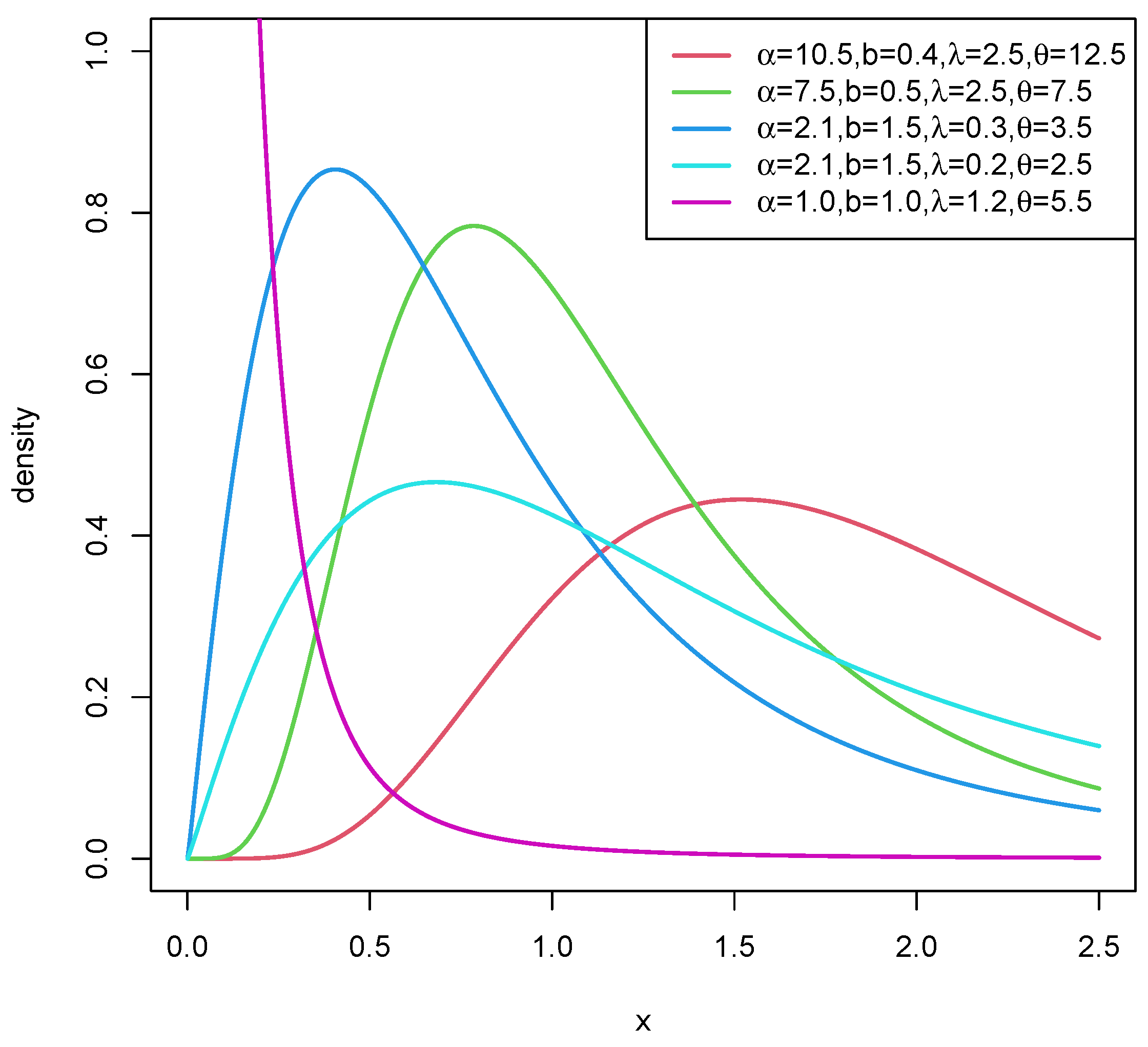
Figure 2.
Fitted Densities and Probability Plots for Failure Times Data.
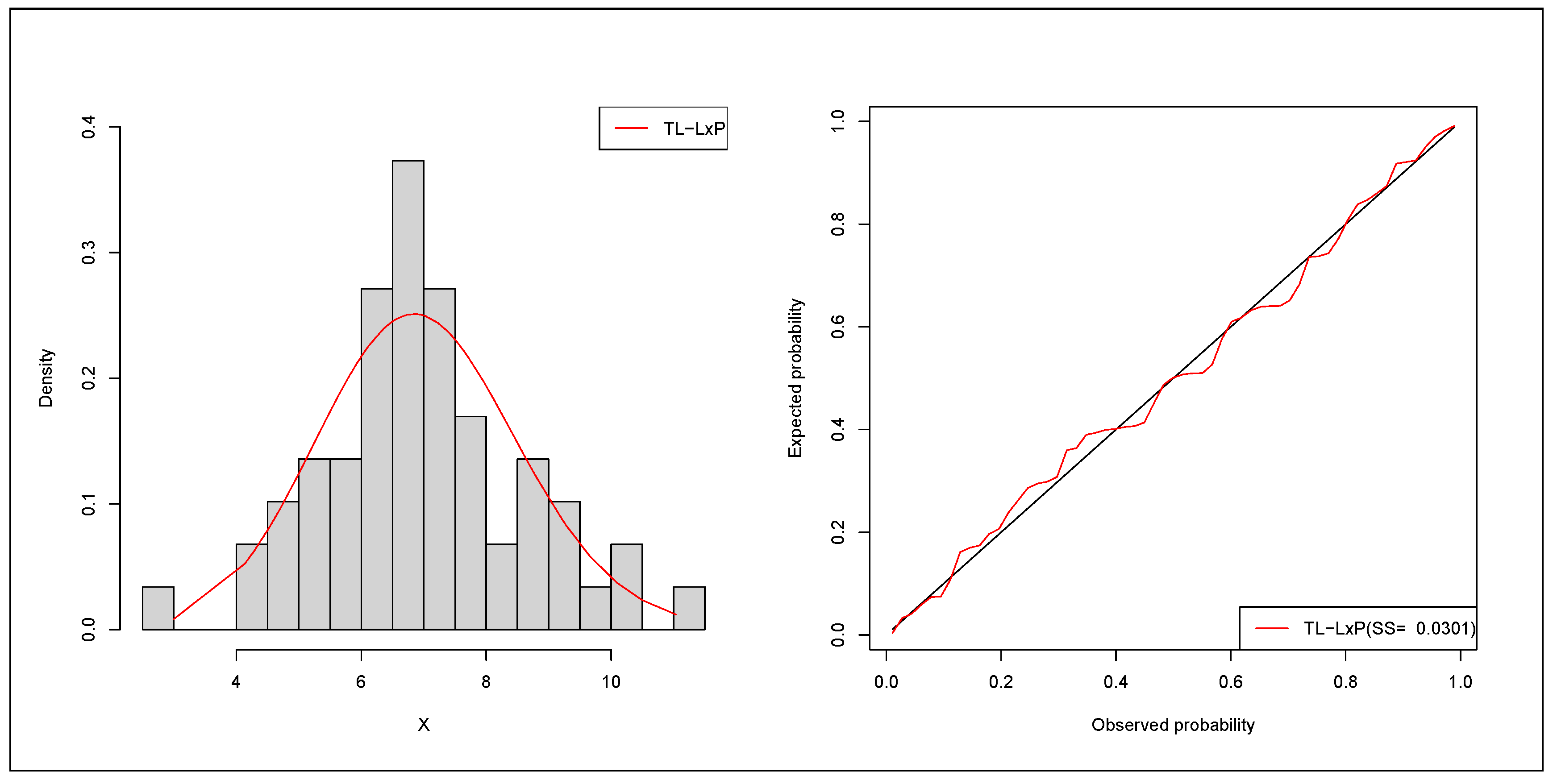
Figure 3.
Fitted K-M and ECDF Plots for Failure Times Data.
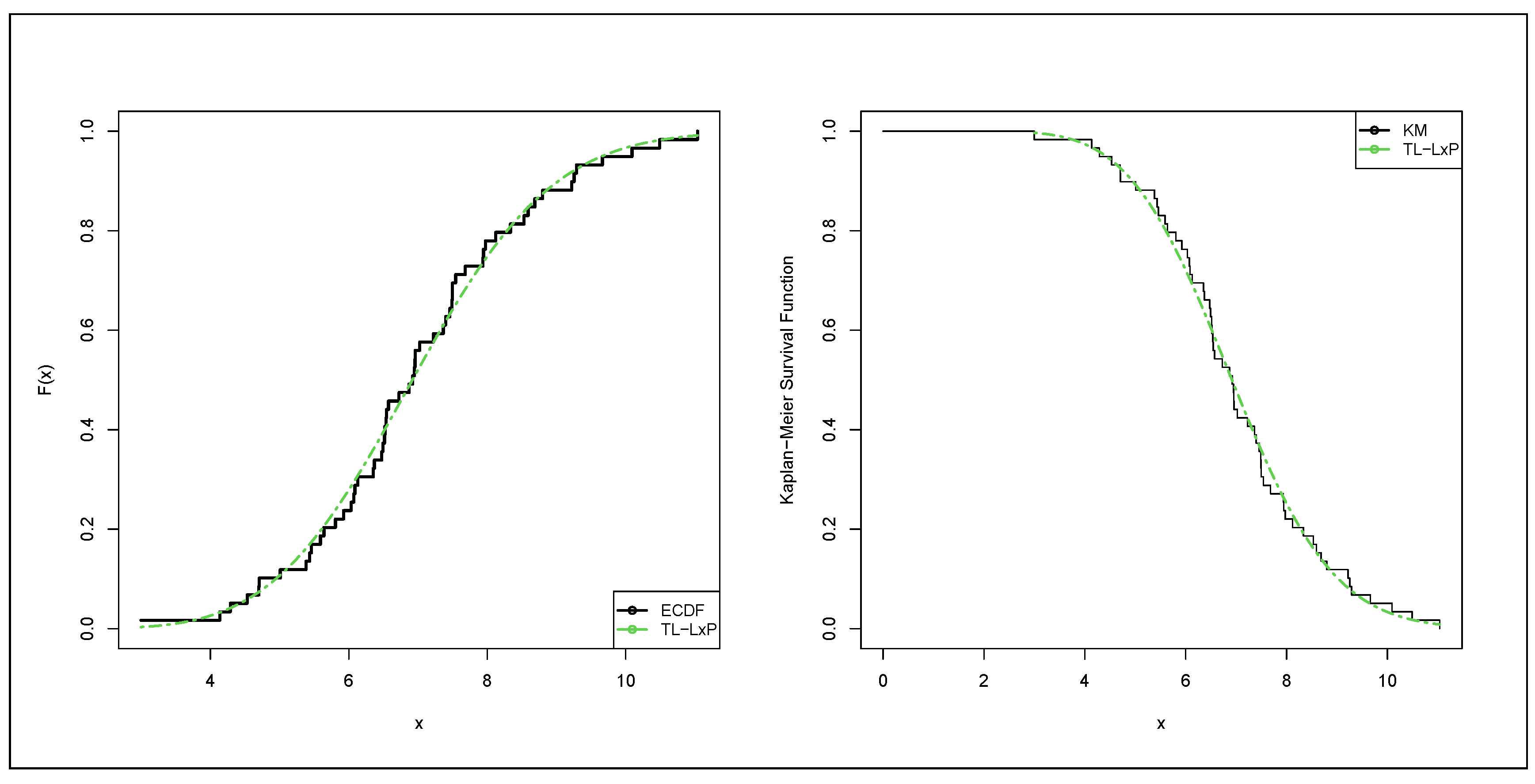
Figure 4.
Fitted TTT and HRF Plots for Failure Times Data.
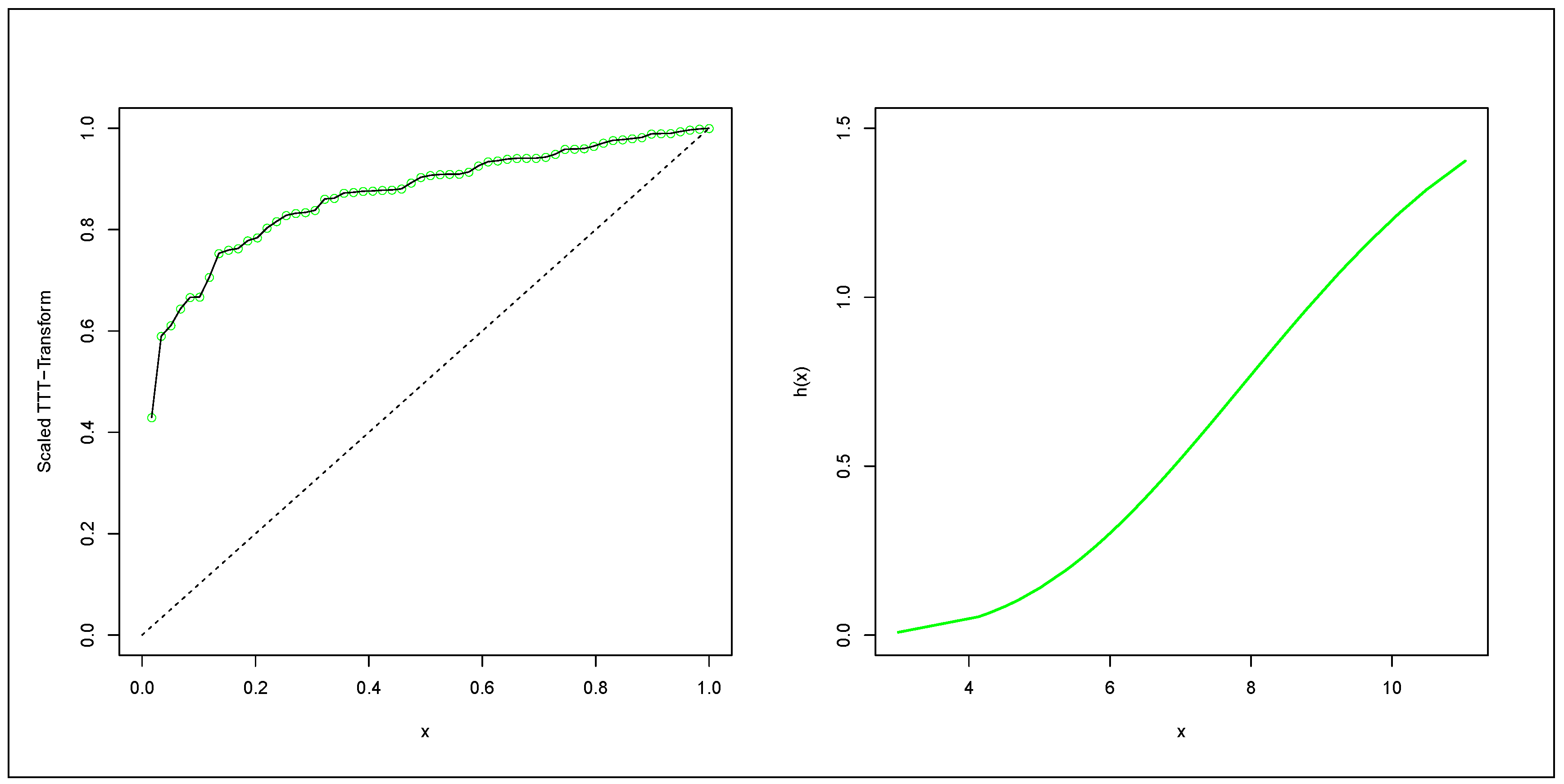
Figure 5.
Fitted Densities and Probability Plots for Red Cells Count Data.
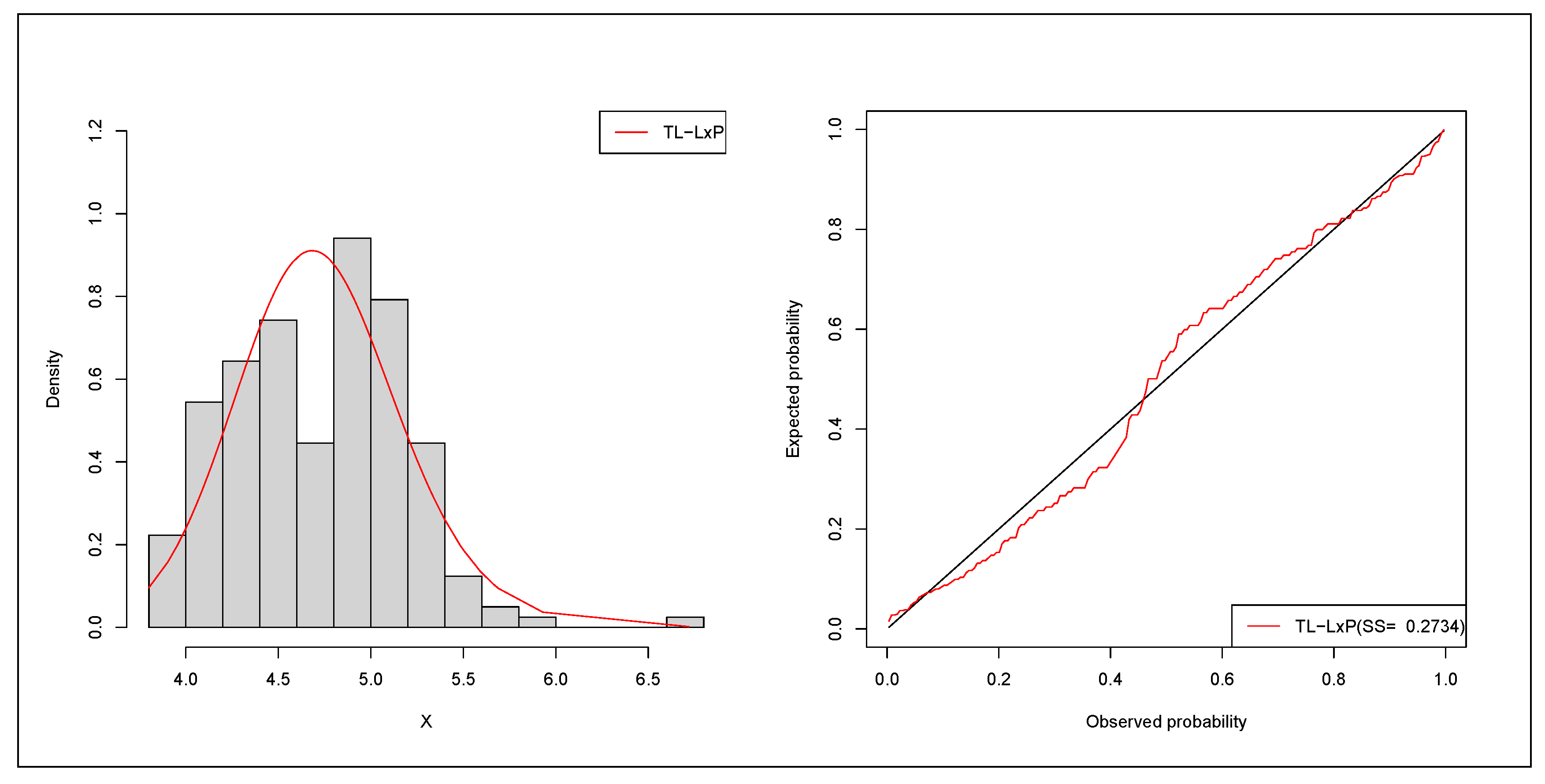
Figure 6.
Fitted K-M and ECDF Plots for Red Cells Data.
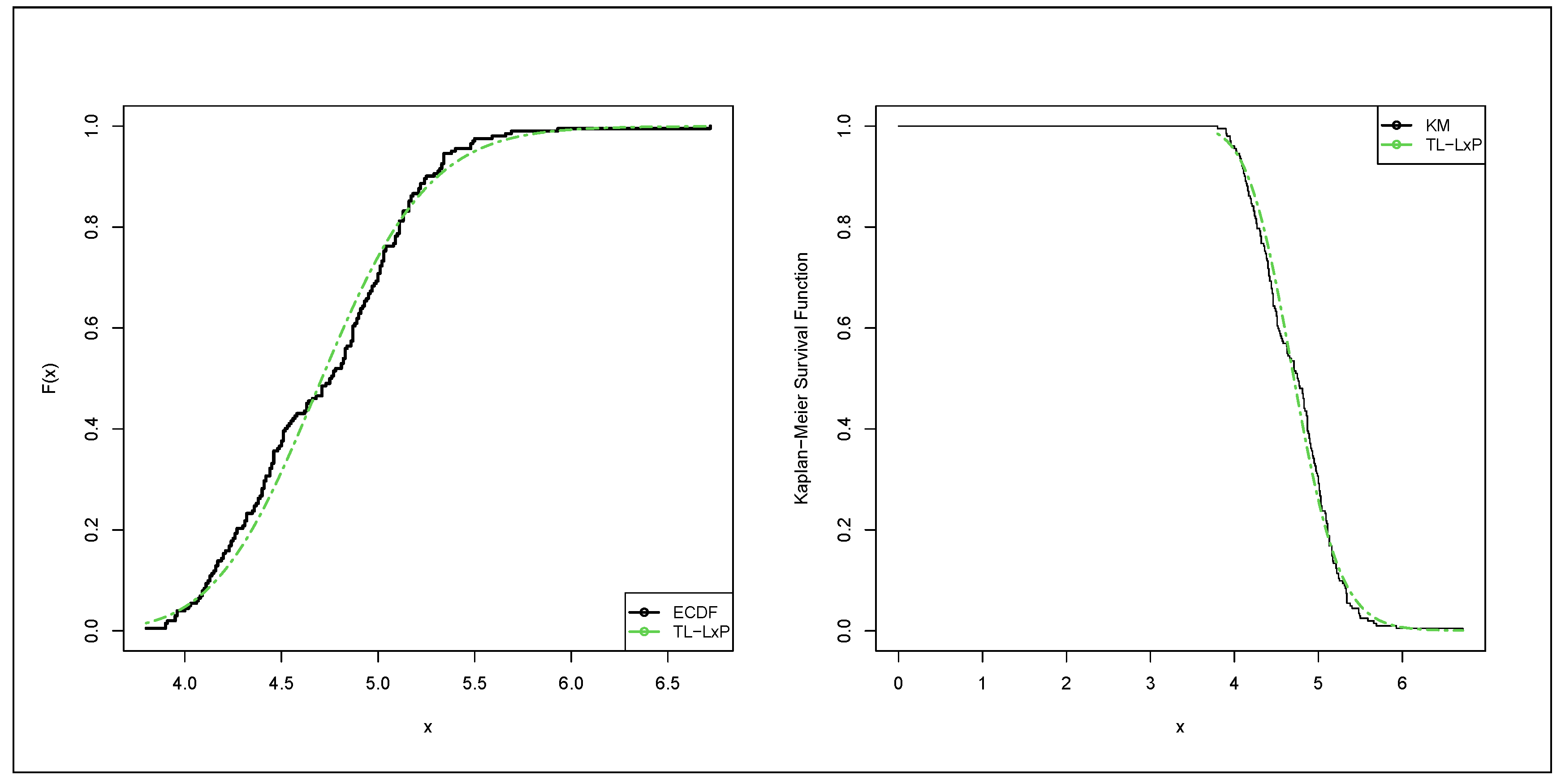
Figure 7.
Fitted TTT and HRF Plots for Red Cells Data.
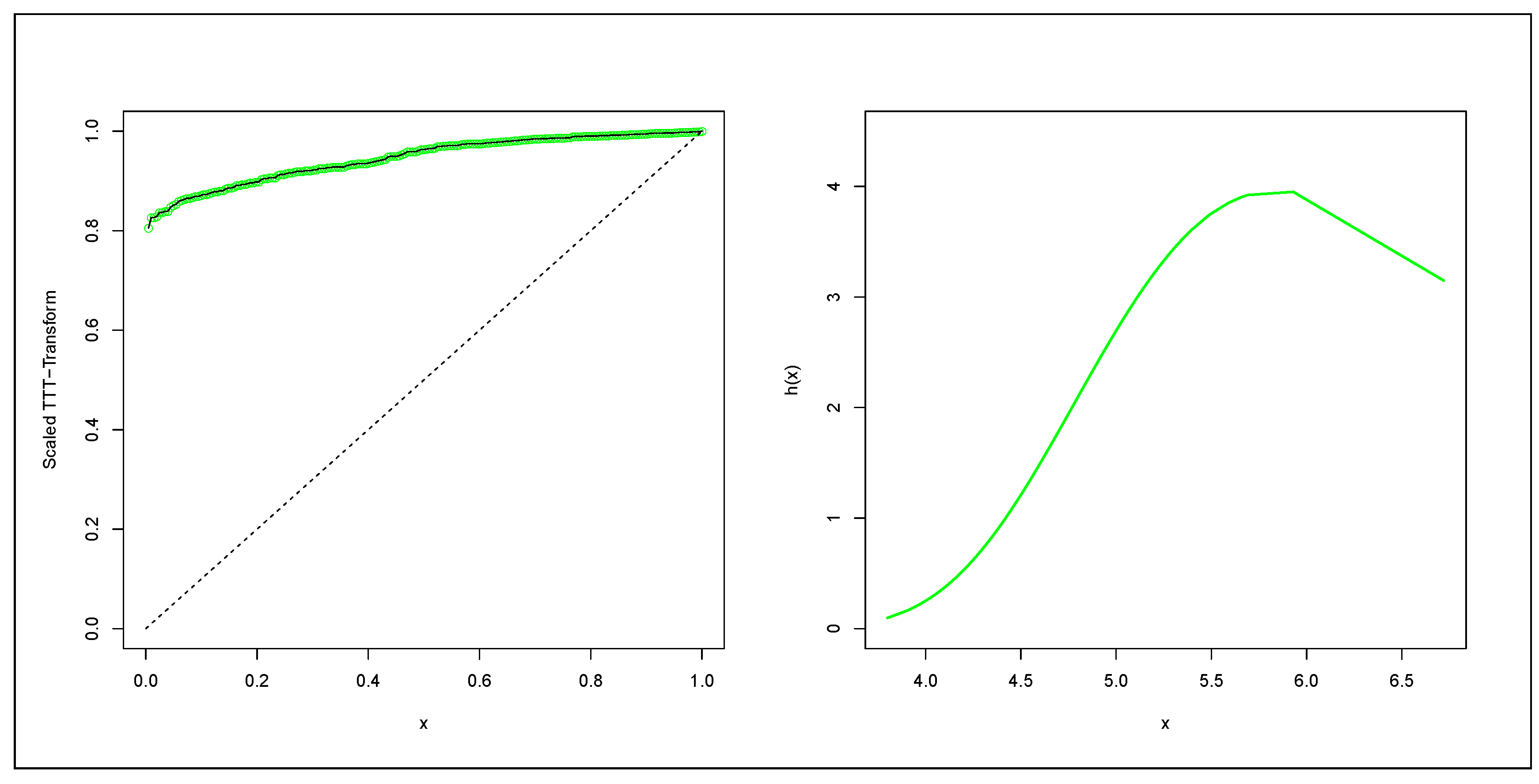
Figure 8.
Fitted Densities and Probability Plots for Acute Bone Cancer Data.
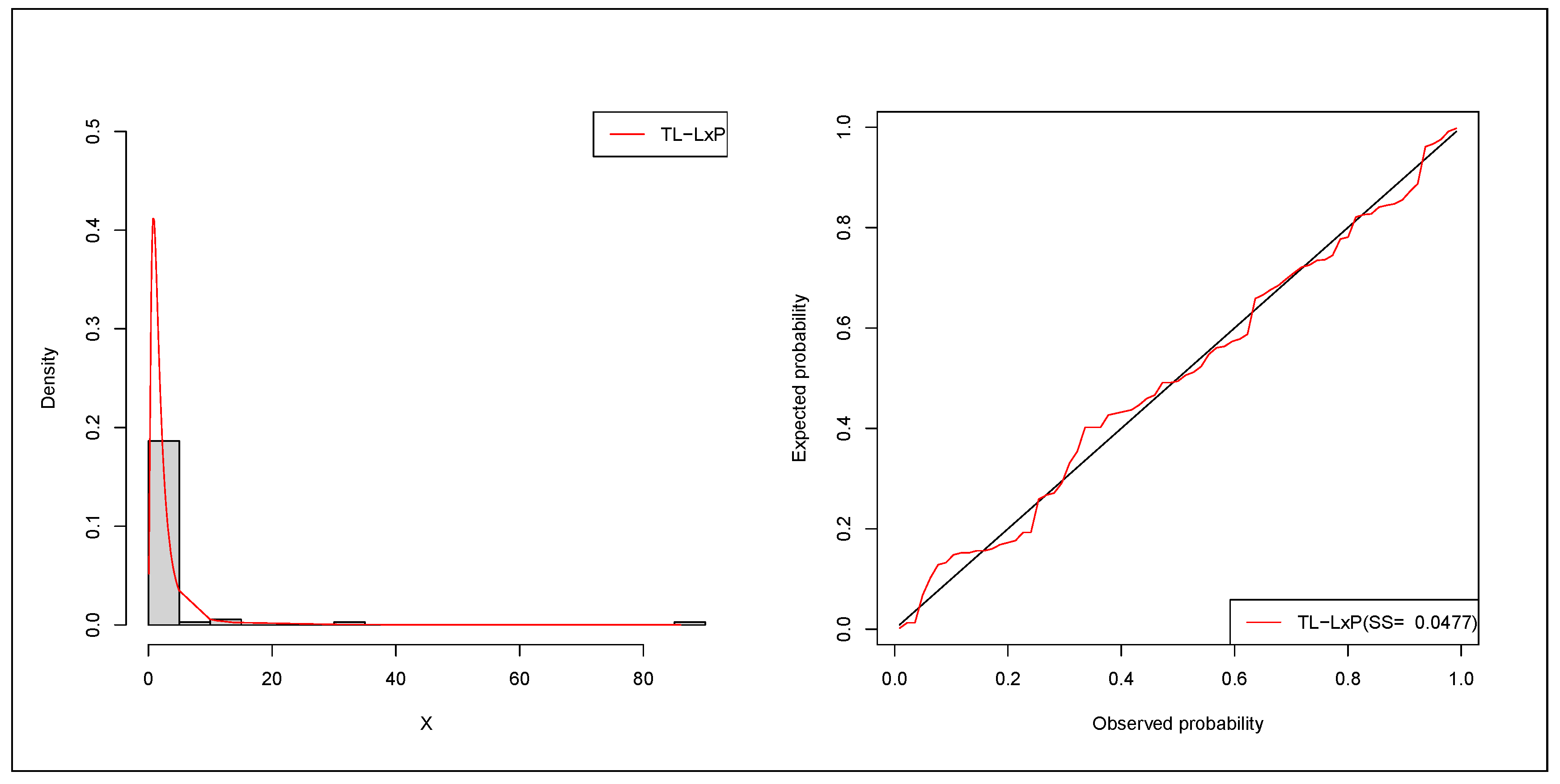
Figure 9.
Fitted K-M and ECDF Plots for Acute Bone Cancer Data.
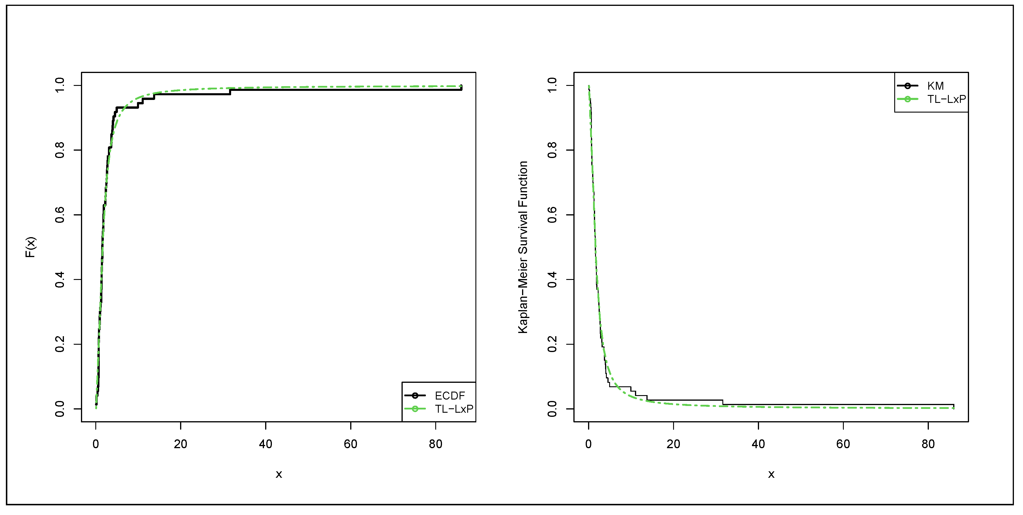
Figure 10.
Fitted TTT and HRF Plots for Acute Bone Cancer Data.
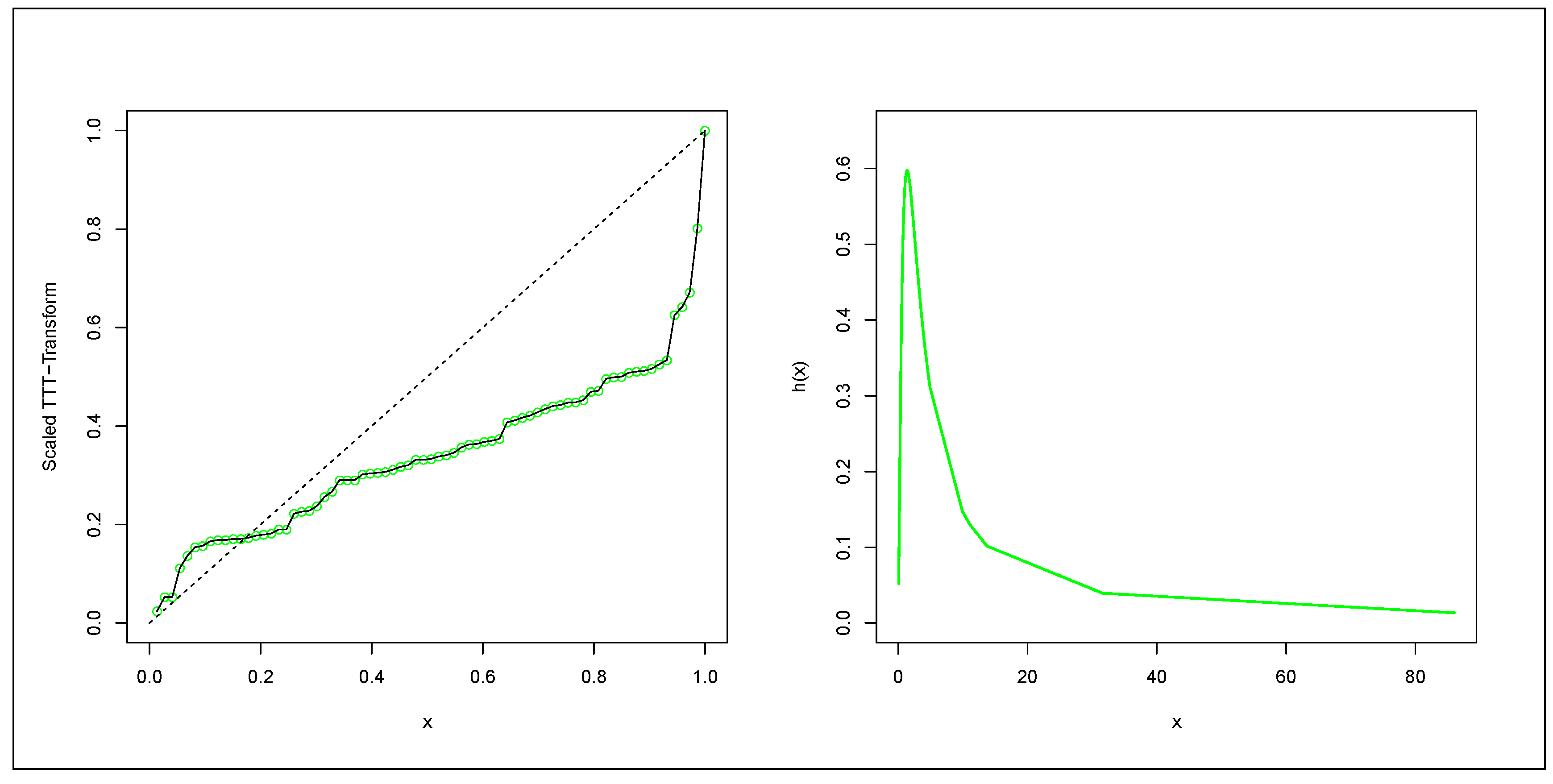

Table 1.
Quantile values for selected parameter values.
| u | (1.5,1.5,0.1,1.5) | (0.5,1,0.5,0.9) | (1.5,0.5,0.3,1.5) | (0.5,1.5,0.9,0.5) | (1.1,1.1,0.3,0.6) |
|---|---|---|---|---|---|
| 0.1 | 0.5267 | 0.00461 | 0.5549 | 0.0024 | 0.1585 |
| 0.2 | 0.9252 | 0.0200 | 1.0134 | 0.0101 | 0.3278 |
| 0.3 | 1.3448 | 0.04923 | 1.5337 | 0.0244 | 0.5264 |
| 0.4 | 1.8225 | 0.0973 | 2.1748 | 0.0472 | 0.7693 |
| 0.5 | 2.3994 | 0.1731 | 3.0212 | 0.0818 | 1.0792 |
| 0.6 | 3.1417 | 0.2929 | 4.2321 | 0.1344 | 1.4967 |
| 0.7 | 4.1807 | 0.4918 | 6.1721 | 0.2176 | 2.1059 |
| 0.8 | 5.8442 | 0.8624 | 9.9251 | 0.3628 | 3.1224 |
| 0.9 | 9.3687 | 1.7807 | 20.8868 | 0.6879 | 5.3899 |
Table 2.
First five moments and measures of dispersion for selected parameter values.
| (1.5,1.5,0.1,1.5) | (0.5,1,0.5,0.9) | (1.1,0.5,0.8,1.5) | (1.5,1.5,0.9,0.5) | (1.1,0.9,0.3,0.6) | |
|---|---|---|---|---|---|
| 0.1208 | 0.1736 | 0.2224 | 0.2903 | 0.1827 | |
| 0.0823 | 0.0873 | 0.1277 | 0.1540 | 0.1139 | |
| 0.0622 | 0.0569 | 0.0878 | 0.1002 | 0.0820 | |
| 0.0498 | 0.0419 | 0.0664 | 0.0730 | 0.0638 | |
| 0.0415 | 0.0331 | 0.0532 | 0.0570 | 0.0521 | |
| SD | 0.2603 | 0.2390 | 0.2797 | 0.2641 | 0.2838 |
| CV | 2.1555 | 1.3770 | 1.2579 | 0.9096 | 1.5535 |
| CS | 2.0333 | 1.6097 | 1.1231 | 0.8146 | 1.3891 |
| CK | 5.7439 | 4.7457 | 3.0822 | 2.7208 | 3.6022 |
Table 3.
Monte Carlo Simulation Results for the TL-LxP Distribution: Mean, RMSE and AB.
| (1, 1, 0.4, 1) | (1.0, 1.1, 0.4, 1.1) | ||||||
| n | Mean | RMSE | Bias | Mean | RMSE | Bias | |
| 40 | 1.1187 | 0.4721 | 0.1187 | 1.1094 | 0.3637 | 0.1094 | |
| 80 | 1.0418 | 0.2124 | 0.0418 | 1.0438 | 0.2134 | 0.0438 | |
| 100 | 1.0287 | 0.1808 | 0.0287 | 1.0268 | 0.1863 | 0.0268 | |
| 200 | 1.0141 | 0.1252 | 0.0141 | 1.0101 | 0.1200 | 0.0101 | |
| 400 | 1.0003 | 0.0886 | 0.0003 | 1.0008 | 0.0886 | 0.0008 | |
| 40 | 3.0728 | 4.6544 | 2.0728 | 3.4046 | 5.1203 | 2.3046 | |
| 80 | 2.1885 | 3.0581 | 1.1885 | 2.5260 | 3.6024 | 1.4260 | |
| b | 100 | 1.8541 | 2.4040 | 0.8541 | 2.2194 | 2.9517 | 1.1194 |
| 200 | 1.3472 | 1.2323 | 0.3472 | 1.6549 | 1.8163 | 0.5549 | |
| 400 | 1.1522 | 0.5702 | 0.1522 | 1.3192 | 0.7852 | 0.2192 | |
| 40 | 0.5926 | 3.1108 | 0.1926 | 0.4847 | 0.6640 | 0.0847 | |
| 80 | 0.3932 | 0.3985 | -0.0068 | 0.4118 | 0.4269 | 0.0118 | |
| 100 | 0.3985 | 0.3761 | -0.0015 | 0.4036 | 0.4167 | 0.0036 | |
| 200 | 0.3823 | 0.2763 | -0.0177 | 0.3832 | 0.2979 | -0.0168 | |
| 400 | 0.3670 | 0.2154 | -0.0330 | 0.3746 | 0.2305 | -0.0254 | |
| 40 | 1.7883 | 1.3726 | 0.7883 | 1.8600 | 1.3326 | 0.7600 | |
| 80 | 1.6869 | 1.2467 | 0.6869 | 1.7232 | 1.2241 | 0.6232 | |
| 100 | 1.6333 | 1.1739 | 0.6333 | 1.7066 | 1.1771 | 0.6066 | |
| 200 | 1.5767 | 1.1279 | 0.5767 | 1.6617 | 1.1304 | 0.5617 | |
| 400 | 1.4849 | 1.0079 | 0.4849 | 1.5532 | 1.0065 | 0.4532 | |
| (1, 1.1, 0.4, 0.9) | (1.0, 1,0, 1.1, 1.1) | ||||||
| n | Mean | RMSE | Bias | Mean | RMSE | Bias | |
| 40 | 1.1179 | 0.4445 | 0.1179 | 1.1161 | 0.4619 | 0.1161 | |
| 80 | 1.0481 | 0.2139 | 0.0481 | 1.0401 | 0.2156 | 0.0401 | |
| 100 | 1.0297 | 0.1878 | 0.0297 | 1.0280 | 0.1891 | 0.0280 | |
| 200 | 1.0156 | 0.1221 | 0.0156 | 1.0100 | 0.1204 | 0.0100 | |
| 400 | 1.0010 | 0.0878 | 0.0010 | 1.0014 | 0.0876 | 0.0014 | |
| 40 | 3.3695 | 4.9285 | 2.2695 | 4.7556 | 8.7554 | 3.7556 | |
| 80 | 2.4850 | 3.3800 | 1.3850 | 3.3262 | 6.3080 | 2.3262 | |
| b | 100 | 2.2942 | 2.9945 | 1.1942 | 2.5351 | 4.6243 | 1.5351 |
| 200 | 1.6291 | 1.6175 | 0.5291 | 1.4946 | 2.0599 | 0.4946 | |
| 400 | 1.3773 | 0.8805 | 0.2773 | 1.1591 | 0.7450 | 0.1591 | |
| 40 | 0.4667 | 0.7443 | 0.0667 | 2.2409 | 19.8829 | 1.1409 | |
| 80 | 0.3895 | 0.4034 | -0.0105 | 1.0952 | 1.1146 | -0.0048 | |
| 100 | 0.3831 | 0.3863 | -0.0169 | 1.1261 | 1.1634 | 0.0261 | |
| 200 | 0.3640 | 0.2778 | -0.0360 | 1.0627 | 0.7570 | -0.0373 | |
| 400 | 0.3461 | 0.2167 | -0.0539 | 1.0402 | 0.6162 | -0.0598 | |
| 40 | 1.7507 | 1.3448 | 0.8507 | 1.9460 | 1.7794 | 0.8460 | |
| 80 | 1.6485 | 1.2425 | 0.7485 | 1.8051 | 1.3196 | 0.7051 | |
| 100 | 1.5747 | 1.1319 | 0.6747 | 1.7437 | 1.2722 | 0.6437 | |
| 200 | 1.5370 | 1.0988 | 0.6370 | 1.6684 | 1.1725 | 0.5684 | |
| 400 | 1.4525 | 0.9974 | 0.5525 | 1.5819 | 1.1029 | 0.4819 |
Table 4.
Parameter Estimates and Goodness-of-Fit Statistics for Failure Times Data.
| Estimates | Statistics | |||||||||
|---|---|---|---|---|---|---|---|---|---|---|
| Model | b | |||||||||
| TL-LxP | 10.6068 | 3.2757 | 0.0291 | 30.7911 | 222.65 | 230.65 | 231.40 | 238.96 | 0.0354 | 0.2003 |
| (1.5962) | (1.0727) | (0.0075) | (0.2066) | |||||||
| TL-Lx | 53.9590 | 154.2200 | 0.0021 | - | 230.05 | 236.05 | 236.49 | 242.28 | 0.1061 | 0.6512 |
| (6.9886 ) | (9.9495 ) | (7.2301 ) | - | |||||||
| Exp-Lx | 53.2240 | - | 0.0015 | 424.1200 | 230.01 | 236.01 | 236.44 | 242.24 | 0.1053 | 0.6467 |
| (3.7181 ) | - | (5.2423 ) | (1.8960 ) | |||||||
| E-Lx | 101.2300 | 155.7100 | 0.0071 | - | 234.90 | 240.90 | 241.34 | 247.13 | 0.2237 | 1.2920 |
| (3.5910 ) | (2.2705 ) | (0.0009) | - | |||||||
| a | b | - | ||||||||
| W-Lx | 9.5584 | 0.2642 | 1.6864 | - | 224.02 | 230.02 | 230.46 | 236.28 | 0.0669 | 0.3739 |
| (9.7424) | (0.3376) | 6.0967 | - | |||||||
Table 5.
Parameter Estimates and Goodness-of-Fit Statistics for Red Cells Data.
| Estimates | Statistics | |||||||||
|---|---|---|---|---|---|---|---|---|---|---|
| Model | b | |||||||||
| TL-LxP | 275.1900 | 18.0300 | 0.0287 | 12.1300 | 252.25 | 260.25 | 260.45 | 273.48 | 0.2756 | 1.4905 |
| (4.6929 ) | (3.2923 ) | (1.9392 ) | (3.9722 ) | |||||||
| TL-Lx | 2.3999 | 7.0413 | 1.5861 | - | 262.89 | 268.89 | 269.01 | 278.82 | 0.4186 | 2.3022 |
| (7.6362 ) | (2.5623 ) | (1.1394 ) | - | |||||||
| Exp-Lx | 2.7839 | - | 3.6145 | 6.2847 | 261.95 | 267.95 | 268.07 | 277.87 | 0.422 | 2.3240 |
| (3.3390 ) | - | (2.5735 ) | (1.4804 ) | |||||||
| E-Lx | 79.4110 | 46.9440 | 3.7495 | - | 343.91 | 349.91 | 359.71 | 353.81 | 0.2664 | 2.1860 |
| (1.0190 ) | (1.6366 ) | (2.6382 ) | - | |||||||
| a | b | - | ||||||||
| W-Lx | 14.1610 | 0.4390 | 0.7813 | - | 293.41 | 299.41 | 299.54 | 309.34 | 0.2224 | 1.8017 |
| (1.1162) | (0.0465) | (0.1648) | - | |||||||
Table 6.
Parameter Estimates and Goodness-of-Fit Statistics for Acute Bone Cancer Data.
| Estimates | Statistics | |||||||||
|---|---|---|---|---|---|---|---|---|---|---|
| Model | b | |||||||||
| TL-LxP | 2.5917 | 0.5558 | 0.5351 | 4.1833 | 278.29 | 286.29 | 286.88 | 295.45 | 0.0568 | 0.4391 |
| (0.7412) | (0.3128) | (0.4295) | (2.0482) | |||||||
| TL-Lx | 3.3768 | 0.9318 | 0.9169 | - | 281.67 | 287.67 | 288.02 | 294.54 | 0.0919 | 0.6886 |
| (1.1532) | (0.2168) | (0.9169) | - | |||||||
| Exp-Lx | 3.3768 | - | 0.9169 | 1.8637 | 281.67 | 287.67 | 288.02 | 294.54 | 0.0919 | 0.6886 |
| (1.1532) | - | (0.5215) | (0.4337) | |||||||
| E-Lx | 0.7659 | 2.6643 | 1.3793 | - | 322.81 | 328.81 | 329.15 | 335.68 | 0.6017 | 3.6470 |
| (9.2412 ) | (3.3325 ) | (1.3220 ) | - | |||||||
| a | b | - | ||||||||
| W-Lx | 1.7750 | 0.2582 | 5.0702 | - | 300.52 | 306.52 | 306.87 | 313.87 | 0.3067 | 1.9958 |
| (0.4286) | (0.0759) | (4.3144) | - | |||||||
Disclaimer/Publisher’s Note: The statements, opinions and data contained in all publications are solely those of the individual author(s) and contributor(s) and not of MDPI and/or the editor(s). MDPI and/or the editor(s) disclaim responsibility for any injury to people or property resulting from any ideas, methods, instructions or products referred to in the content. |
© 2024 by the authors. Licensee MDPI, Basel, Switzerland. This article is an open access article distributed under the terms and conditions of the Creative Commons Attribution (CC BY) license (http://creativecommons.org/licenses/by/4.0/).
Copyright: This open access article is published under a Creative Commons CC BY 4.0 license, which permit the free download, distribution, and reuse, provided that the author and preprint are cited in any reuse.


