Copula-Based Risk Aggregation and the Significance of Reinsurance

1. Introduction

Determining the level of capital required for business continuity is essential for insurance companies. The interest in the literature concerning the significance of capital requirements is increasing, as evidenced by the studies by [9,15,24,39], and most recently [33]. The capital which is mostly referred to as capital requirement or business capital should support an insurance company minimizing the risk of insolvency and serving its obligations to the policyholders. When extreme events happen, such as floods, earthquakes, hurricanes and other catastrophic events, the claims amount to be paid by an insurance company can be extremely high. However, part of the claims can be passed to reinsurance companies. An insurance company (cedent) can transfer some risks to another insurer (the reinsurer) exchanging part of its unexpected future losses by the payment of a fixed premium.

Typically the cedent insurance company keeps most of the risk and when large amounts of claims occur, these can originate not just from one business line but involve other products as well. In other words, some insurance business lines are dependent on each other, in the sense that an increase on the claims amount being filled in one business line is accompanied by a higher claims amount in other business lines too. In addition, these claims due to correlated catastrophic events could lead to defaults in insurance system ([27,48]). Therefore, it is essential for regulators to monitor these issues. To the best of our knowledge, the interaction between two critical aspects of insurance—dependence among risks and partial risk cession—remains underexplored. This study addresses this gap by evaluating the impact of reinsurance on the composition and risk profile of an insurer’s portfolio across multiple business lines. Leveraging flexible copula models and portfolio diversification metrics, we analyze empirical data from the Australian insurance market to quantify these effects. Our findings provide actionable insights for policymakers, enabling them to design more effective strategies for the reinsurance industry and enhance systemic stability.

Aggregating the risk of losses for insurance companies is challenging. The most crucial aspect of the aggregation process is modelling the dependence structure between the risks of losses across different business lines. Examining linear correlations is a classic approach to model risk dependence but fails to incorporate all possible dependence structures. The use of the classic multivariate Gaussian model implicitly assumes symmetry between the multivariate tails and a linear relationship between variables. To investigate potential non-linearities, for instance, whether losses are more strongly related than gains in financial data, we use copula models, which can be seen as a generalization of the classic multivariate Gaussian model. When selecting a copula model, if the multivariate Gaussian is the most appropriate distribution, then it will still be the chosen model. In the case of insurance claims, we must consider the possibility of asymmetries and non-linearities. Small claims might originate more independently from each other, while very large claims might have underlying common causes (e.g., weather related events) and thus exhibit stronger dependence. When linearity and symmetry may not hold, copulas are the appropriate method to model the dependence structure. Copulas have received increasing interest from researchers and practitioners in recent years.

This paper is twofold. First, we focus on modelling the aggregation of risks from different business lines in insurance. Second, we then explore the effect of reinsurance on the level of risks and how this relates with the dependence structure between different business lines. To model the multivariate structure the insurance risks, we use a hierarchical risk aggregation method based on two dimensional copulas. As an alternative to hierarchical copulas one could use vine copula models ([19,30]. But these may not perform as well as hierarchical copulas when some variables, more strongly related than others, form natural groups inherent to the specific application [12]. However, hierarchical copulas may outperform vine copulas when certain variables, which are more strongly related than others, form natural groups inherent to the specific application. If we ignore the particular application, both methods can be used to model multivariate distributions. These two procedures have been compared in [37] from a purely probabilistic point. In our study, fire and house insurance claims are expected to be strongly related, as are liability and CTP* (Compulsory Third Party liability) insurance claims. This natural hierarchical dependence is confirmed in our data analysis, justifying our choice of the hierarchical copula methodology.

The hierarchical risk aggregation approach recently adopted by [17] developed by [6]. The hierarchical aggregation procedure, is based on rooted trees that include branching and leaf nodes, and uses the elliptical copula family for each aggregation step. However, as highlighted by in [22], this copula family has certain drawbacks, such as its inability to capture dependence structures, which are not radially symmetric. Especially in the case of extreme events, the dependence of large losses from different business lines cannot be modelled by the elliptical copula family (see [39]).

In this paper, we address this issue by proposing a novel hierarchical framework that integrates copulas from the Archimedean family. Archimedean copulas offer inherent asymmetry and flexibility to model diverse dependence structures, particularly in tail dependencies. To further enhance adaptability, we incorporate mixtures and rotated variants of Archimedean copulas, selected through rigorous goodness-of-fit tests to match empirical data patterns. This dual approach—combining hierarchical aggregation with Archimedean-based copulas—represents a key innovation, enabling robust risk modeling without relying on restrictive conditional assumptions.

For the empirical application, we use data from the Australian Prudential Regulation Authority (APRA). Modelling insurance claims for capital requirements using Australian data is not only relevant for Australian insurers but also for insurers based on other countries. While Solvency II establishes the capital requirements in Europe, similarly APRA’s GPS Prudential Standards regulate insurer’s capital requirements in Australia. Solvency II establishes the equivalence between the two supervisory frameworks which is essential for European insurers operating in Australia. Hence, the methodology and results from this study are relevant for all countries with regulatory equivalence under Solvency II.

[46] analize APRA’s data consisting of 19 semi-annual gross incurred claims and earned premiums from December 1992 to June 2002. We choose to use more recent data with a quarterly frequency in order to increase the sample size and improve the estimation of the risk aggregation model. As a result, a total of 28 observations, consisting of quarterly premiums earned and incurred claims, gross and net of reinsurance, for five business lines, were selected for the period between September 2010 and June 2017. The quarterly incurred claims and premiums earned are then used to calculate loss ratios for the five different business lines. The risk aggregation model is selected based on the resulting loss ratios, measuring the associated risks. The gross and net of reinsurance loss ratios are used to examine the change in the level of risk for each business line and for the aggregate risk.

Research on risk aggregation with copulas applied to insurance was pioneered by [49]. This research introduces the concept of copula and chooses Gaussian copula as one of the useful tools in determining the risk aggregation of an insurance company by combining correlated loss distributions. More specifically, the aggregate loss distribution is determined by the combination of the effect from claim frequency and claim severity distribution. By contrast, [46] use copula models to aggregate risks in order to determine the economic capital as well as the diversification benefits focusing on the insurance industry. Using multiple insurance business lines data, they analyse the importance of selecting an appropriate copula model to avoid underestimation or overestimation of capital required, which consequently may affect the level of capital for insurance products. [11] highlight that modelling the dependence between risks is important as it is a form of rule for risk aggregation. Their research also consider various methods to model dependencies, which subsequently affect the diversification benefits and show that overestimation of diversification may cause inaccurate computation of risk-based capital (RBC). [39] use copulas to cover the loopholes of Solvency II, such as linear correlations being used to measure the dependence structure of correlated risks. However, a linear correlation may not be suitable for modelling dependence structure and may not be able to capture all information of a tail distribution. To overcome this problem, the authors propose a method of risk aggregation via copula to determine the dependence structure between risks. Nevertheless, their focus is from the perspective of the Solvency II, rather than on the risk aggregation modelling based on real data.

Modelling risk aggregation using a dimensional copula can be very challenging and requires more parameters to be estimated than the traditional two dimensional copula or bivariate copula models [11]. With this in mind, we consider hierarchical aggregation as an alternative modelling technique, based on two dimensional copula for high dimensional copulas. This model, introduced by [6], has an advantage where it does not requires specification of copula for all business lines. Instead, a copula and the joint dependence between the aggregated sub-business lines will be determined in each aggregation step. The aggregation model is represented by a rooted tree, which consists of branching nodes and leafs based on graph theory.

In addition, we also investigate the significance of reinsurance from the risk management perspective. Insurance companies are able to transfer risks to reinsurance and as a result capital is saved from being allocated to these risks [8]. Previous research by [18] proves that insurance companies purchase reinsurance for the benefits of reducing the loss ratio measured by its volatility. It also provides protection against catastrophes by limiting the liability on specific risks. The drawback of reinsurance is that insurers’ cost for production is increased. Furthermore, reinsurance also provides other benefits, such as capital relief as well as flexible financing. In our study, we use two measures of portfolio diversification, where portfolio is defined as a collection of insurance business lines. The first measure of diversification is derived from [42] entropy, while the second was introduced in [13]. While the first measure concentrates on the weights of the business lines, the second one focuses on the risk of the portfolio. In our empirical analysis of Australian insurance data, we find that, although the portfolio of business lines without reinsurance is more balanced and hence more diversified according to Shannon’s measure, reinsurance reduces the risk of the (reinsured) portfolio, thereby increasing diversification according to Choueifaty and Coignard’s measure.

The remaining of this paper is organized as follows. Section 2 discusses the methods for aggregating risk using hierarchical copula aggregation model, copula simulations and determination of capital requirement. Section 3 contains the estimation of the hierarchical aggregation copula model and analysis of the results. In Section 4 we study the effects of reinsurance in the level of risk and diversification of the portfolio of different business lines. Section 5 concludes the paper.

2. Copula-Based Hierarchical Aggregation Model

In finance and insurance popular models for problems involving a large number of random variables have been based on copula functions. Different copula models have been proposed. These include Archimedean and elliptical copula models [25], vine copula models ([1,32]), and hierarchical copula models [16,17,34].

While some of these models impose restrictive dependence structures, complicating inference, vine copulas—despite their growing popularity—require a critical assumption: each conditional bivariate copula must be independent of the conditioning variable, except through its marginal distributions [28]. This assumption, while essential for accurate inference, limits their applicability in practice. In contrast, hierarchical copulas eliminate the need for conditional copulas entirely, avoiding such assumptions. Their straightforward structure requires only a single copula and corresponding joint dependence at each aggregation step, significantly simplifying estimation. In this study, we adopt hierarchical copulas to strike an optimal balance between ease of estimation and model flexibility, offering a robust alternative to more complex approaches. This article adopts the hierarchical copula model with the goal of achieving a good compromise between ease of estimation and flexibility.

2.1. The Definition of Copula

Bivariate copulas are the main building block of hierarchical aggregation copula models. Here we only provide the basic definition in order to introduce the notation and we refer the reader to [38] and [35] for an introduction to copulas and the definition of specific copula families.

Given a d-dimensional random vector ${(X_1,X_2,\dots ,X_d)}^{\prime }$, 1 from [44] there exists a function $C:{[0,1]}^d\to [0,1]$ such that

$$\mathbb{P}(X_1\le x_1,X_2\le x_2,\dots ,X_n\le x_d)=C(F_1\left(x_1\right),F_2\left(x_2\right),\dots ,F_d\left(x_d\right)),$$

where $F_i\left(x\right)=\mathbb{P}(X_i\le x_i)$ is the cumulative distribution function (cdf) of $X_i$ for $i=1,2,\dots ,d$, and C is a copula function. In fact, a copula is a multivariate joint cdf with uniform margins. If the univariate cdf’s $F_i$ are continuous then the copula function C is unique.

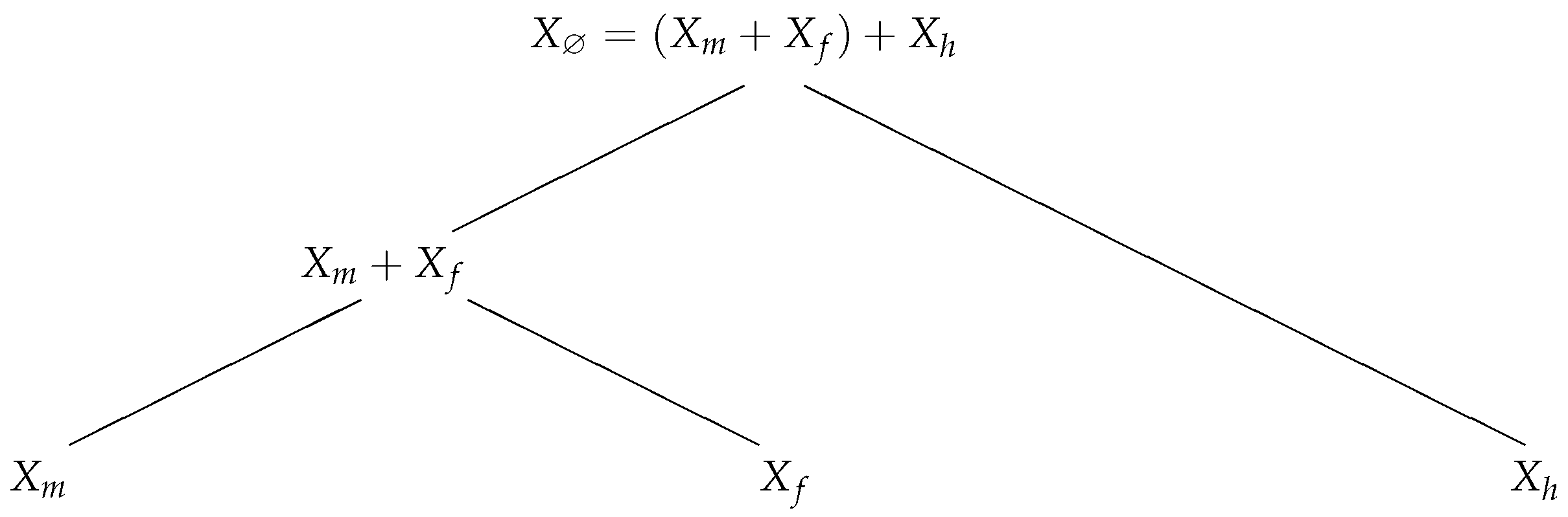
2.2. Hierarchical Aggregation Copula Models

Hierarchical copula models draw on results from graph theory on rooted trees [21]. Following the notation used in [6], a rooted tree $\tau$ is composed by leaf nodes and branching nodes where one of the branching nodes is the root. The subset of branching nodes is denoted by $ℬ$ $\left(\tau \right)$, the subset of leaf nodes is denoted by $ℒ$ $\left(\tau \right)$, and the root node by ⌀. Naturally, $ℬ$ $\left(\tau \right)\cup$$ℒ$ $\left(\tau \right)=\tau$ and $ℬ$ $\left(\tau \right)\cap$$ℒ$ $\left(\tau \right)=\varnothing$. In order to use rooted trees to aggregate the losses of several business lines we make the following assumptions:

• Each leaf node in the rooted tree is associated with the loss of business line i, represented by a random variable $X_i$.
• Each branching node is associated with the sum of the business lines mapped to that node’s children.

In Figure 1 we illustrate the mapping to a rooted tree of three insurance loss random variables $X_m$, $X_f$ and $X_h$ representing the business lines Motor, Fire and Household, respectively. Each leaf node corresponds to a business line and each branching node corresponds to the sum of the variables associated with its children leaf nodes. As in [6], we assume that each branching node has two children for simplicity, although the results on rooted trees used in this paper are valid for branching nodes with any number of children (see [6]). By assuming that each branching node has only two children, we can simplify the construction and estimation of the model as only bivariate copulas are involved. In order to define the aggregation model we denote by ${\left(X_i\right)}_{i\in T}^{\prime }={(X_1,X_2,\dots ,X_d)}^{\prime }$ the vector of random variables, where each $X_i$ represents the loss of the business line i. The rooted tree aggregation model for the random vector ${\left(X_i\right)}_{i\in \tau }$ is determined by

• a rooted tree structure $\tau$,
• univariate cdf’s $F_i:\mathbb{R}\to [0,1]$ for all leaf nodes i in $ℒ$ $\left(\tau \right)$, and
• bivariate copula functions $C_j:{[0,1]}^2\to [0,1]$ for the two children of each branching node j in $ℬ$ $\left(\tau \right)$.

We denote the tree aggregation model by $(\tau ,{\left(F_i\right)}_{i\in ℒ\left(\tau \right)},{\left(C_j\right)}_{j\in ℬ\left(\tau \right)})$. Using this modelling approach we obtain the distribution of the root node which represents the aggregate total loss

$$X_{⌀}=X_1+X_2+\dots +X_d=\sum _{i\in ℒ\left(\tau \right)}{X}_i$$

based on the univariate cdf’s for the business lines associated with the leaf nodes, and the bivariate copulas associated with the branching nodes.

2.2.1. Existence and Uniqueness of a Joint Distribution

The existence and uniqueness of the joint distribution of the hierarchical aggregation copula model for the vector ${(X_1,X_2,\dots ,X_d)}^{\prime }$ have been studied in [6]. Here we only summarise the conditions and the main results necessary in this paper. Given a rooted tree aggregation model $(\tau ,{\left(F_i\right)}_{i\in ℒ\left(\tau \right)},{\left(C_j\right)}_{j\in ℬ\left(\tau \right)})$ where each branching node $j\in$$ℬ$ $\left(\tau \right)$ is the sum of its children, the random vector ${\left(X_i\right)}_{i\in \tau }$ is called a mildly tree dependent. A mildly tree dependent random vector ${\left(X_i\right)}_{i\in \tau }$ is called tree dependent if for each branching node $i\in ℬ\left(\tau \right)$, given $X_i$, its descendants ${\left(X_j\right)}_{j\in 𝒟\left(i\right)}$, where $𝒟\left(i\right)$ is the set of descendent nodes, are conditionally independent of the remaining nodes ${\left(X_j\right)}_{j\in \tau \setminus 𝒟\left(i\right)}$, that is

$${\left(X_j\right)}_{j\in 𝒟\left(i\right)}\perp {\left(X_j\right)}_{j\in \tau \setminus 𝒟\left(i\right)}|X_i\mathrm{for}\mathrm{all}i\in ℬ\left(\tau \right).$$

This conditional independence condition however does not imply that ${\left(X_j\right)}_{j\in 𝒟\left(j\right)}$ is independent of ${\left(X_j\right)}_{j\in \tau \setminus 𝒟\left(i\right)}$, because their dependence may come from $X_i$.

Theorem 1. 

Given a rooted tree aggregation model $\left(\tau ,{\left(F_i\right)}_{i\in ℒ\left(\tau \right)},{\left(C_j\right)}_{j\in ℬ\left(\tau \right)}\right)$, a tree dependent random vector exists and its joint distribution is unique.

For the proof of this result see [6]. For the example illustrated in Figure 1 the joint distribution of the hierarchical aggregation copula model for the vector ${(X_m,X_f,X_h)}^{\prime }$ exists and is unique if and only if

$$(X_m,X_f)\perp (X_{⌀},X_h)|X_m+X_f,$$

where $X_{⌀}=X_m+X_f+X_h$. This means that all the information in $X_m$ and $X_f$ that influences $X_h$ is contained in $X_m+X_f$.

Under the above theorem, if all the univariate and copula distributions are absolutely continuous then the joint density function is given by the following proposition showed in [17].

Proposition 1. 

Given a rooted tree aggregation model $(\tau ,{\left(F_i\right)}_{i\in ℒ\left(\tau \right)},{\left(C_j\right)}_{j\in ℬ\left(\tau \right)})$ with d leaf nodes associated with the vector $\mathbf{X}={(X_1,X_2,\dots ,X_d)}^{\prime }$, the joint density function of the vector $\mathbf{X}$ is given by

$$f_{\mathbf{X}}(x_1,\dots ,x_d)=\prod _{j=1}^{d-1}{c}_j\left[F_{\mathrm{LD}\left(j1\right)}\left(\sum _{i\in \mathrm{LD}\left(j1\right)}{x}_i\right),F_{\mathrm{LD}\left(j2\right)}\left(\sum _{i\in \mathrm{LD}\left(j2\right)}{x}_i\right)\right]\prod _{i=1}^d{f}_i\left(x_i\right),$$

for all $x_1,\dots ,x_d\in \mathbb{R}$, where $\mathrm{LD}\left(ji\right)$ represents the leaf nodes in the set of descendants of child node i of the branching node j, $F_{\mathrm{LD}\left(jk\right)}$ is the cdf of the sum of the leaf nodes in $\mathrm{LD}\left(jk\right)$, $f_1,\dots ,f_d$ are the univariate density functions of $X_1,X_2,\dots ,X_d$ respectively, and $c_j$ is the copula density function of the children of $X_j$ for $j\in ℬ\left(\tau \right)$.

As an example, for the business lines represented by the random vector ${(X_m,X_f,X_h)}^{\prime }$ associated with the rooted tree $\tau$ illustrated in Figure 1 the joint density function is given by

$$\begin{array}{c}{f}_{\mathbf{X}}(x_m,x_f,x_h)=c_{m,f}\left(F_m\left(x_m\right),F_f\left(x_f\right)\right)c_{m+f,h}\left(F_{m+f}(x_m+x_f),F_h\left(x_h\right)\right)\hfill \\ \hfill .f_m\left(x_m\right)f_f\left(x_f\right)f_h\left(x_h\right),\end{array}$$

for all $(x_m,x_f,x_h)$, where $F_i$ is the cdf of the univariate random variable $X_i$ with density function $f_i$, $F_{m+f}$ is the cdf of $X_m+X_f$, $c_{m,f}$ is the copula density function of $(X_m,X_f)$ and $c_{m+f,h}$ is the bivariate copula density function of $((X_m+X_f),X_h)$.

2.2.2. Simulation of Joint Distributions

Given the set of d business lines represented by the random variables $X_1,X_2,\dots ,X_d$, we determine the tree structure by aggregating iteratively the pair of variables with the strongest dependence. We use Kendall’s tau to measure the dependence between pairs of random variables in the hierarchical aggregation procedure. For the motivation and justification for using Kendall’s tau in this setting see [17].

After defining the structure of the tree we proceed with selecting the probability distribution for the random variable allocated to a leaf node and the copula family for the two children of each branching node in order to specify the hierarchical aggregation model. We use maximum likelihood estimation to estimate the parameters, and [5,26] goodness-of-fit methods to select the best probability distributions.

The hierarchical aggregation model allows to estimate measures of risk on the sum of the individual variables considered. We estimate these risk measures based on the simulation of observations from the aggregation model. By generalising the algorithm introduced in [6] that consists of a numerical approximation procedure where sample reordering induces the dependence structure, a technique that goes back to the work of [29].

We present below the algorithm for the case when all branching nodes have two children and the functional that produces the aggregation is a weighted sum of the branching nodes. [10] generalize the case when the aggregation functionals are Kendall functions.

Sample Reordering Numerical Approximation Algorithm

• Define the number of simulations $N\in \mathbb{N}$.
• Simulate N independent samples from the univariate random variables $X_i$ ($i\in ℒ\left(\tau \right)$) associated with d leaf nodes: $X_i^k\sim F_i$ for $k=1,\dots ,N$ and $i=1,\dots ,d$, where $F_i$ is the pre-determined univariate cdf for $X_i$.
• Simulate N independent samples from the bivariate copula $C_j$ ($j\in ℬ\left(\tau \right)$) associated with each of the $d-1$ branching nodes: ${\mathbf{U}}_j^k=(U_{j1}^k,U_{j2}^k)\sim C_j$ for $k=1,\dots ,N$ and $j=1,\dots ,d-1$.
• Following a bottom-up approach, beginning at the branching nodes closer to the leaf nodes and ending at the root nodes define the approximation for the cdf of each branching node $j\in ℬ\left(\tau \right)$ as

  $$F_j^N\left(x\right)={\displaystyle \frac{1}{N}}\sum _{k=1}^N\mathbb{1}\left\{w_{j1}{x}_{j1}^{\left(r_{j1}^k\right)}+w_{j2}{x}_{j2}^{\left(r_{j2}^k\right)}\le x\right\},$$

  recursively, where $\mathbb{1}$ is the indicator function2, $x_{j1}^k$ and $x_{j2}^k$ are (simulated) sample values of the random variables associated with the two nodes children of the branching node j, $w_{ji}$ is the weight given to variable $X_{ji}$, $r_{ji}^k$ is the (componentwise) rank of $u_{ji}^k$, and $\{x_{ji}^{\left(1\right)},x_{ji}^{\left(2\right)},\dots ,x_{ji}^{\left(N\right)}\}$ , $i=1,2$ are the ordered sample.

Once we have the estimate for the cdf of the total aggregate loss we proceed estimating the risk measures of interest.

2.3. Risk Estimation of the Aggregate Loss

After building the model for the aggregate loss, using the hierarchical copula model we can estimate the risk of the aggregate loss. In the process of risk aggregation, the bivariate copula is used to link every two losses, such as $X_1$ and $X_2$. TVaR is then applied to estimate the risks of the aggregate losses. TVaR is used to fulfil the coherent risk measure property as suggested by [2,3] and [7]. The TVaR of the loss represented by the random variable X at the confidence level $\alpha$, for $\alpha \in (0,1)$, is defined as

$${\mathrm{TVaR}}_{\alpha }\left(X\right)={\displaystyle \frac{1}{1-\alpha }}{\int }_{\alpha }^1{\mathrm{VaR}}_u\left(X\right)du,$$

where the ${\mathrm{VaR}}_{\alpha }$ of the random loss X is given by

$${\mathrm{VaR}}_{\alpha }\left(X\right)=inf\left\{x\in \mathbb{R}:P(X\le x)\ge \alpha \right\}.$$

Conventionally, $\alpha$ typically takes the values 90%, 95% or 99%. In order to estimate the TVaR we use the following nonparametric estimator that can be found in more detail in [4]. Given n observations $\{x_1,x_2,\dots ,x_n\}$ of the variable X the TVaR estimator is given by

$${\widehat{\mathrm{TVaR}}}_{\alpha }={\displaystyle \frac{1}{n(1-\alpha )}}\left(\sum _{i=1}^{\lfloor n(1-\alpha )\rfloor }{x}_{(n-i+1)}+(n(1-\alpha )-\lfloor n(1-\alpha )\rfloor )x_{(n-\lfloor n(1-\alpha )\rfloor )}\right),$$

(1)

where $\{x_{\left(1\right)},x_{\left(2\right)},\dots ,x_{\left(n\right)}\}$ is the ordered sample, $\lfloor v\rfloor$ denotes the largest integer not greater than v. In our setting, we estimate the TVaR by applying Eq.(1) to the N observations simulated by the sample reordering algorithm. Given its wide use by insurance regulators, we also report the VaR estimates for the three commonly used confidence levels VaR below.

2.4. The Data

The data on general insurance are obtained from the Australian Prudential Regulation Authority (APRA) (https://www.apra.gov.au/) as also used by [46]. However, we use a more recent time period and quarterly data instead of annual data to increase the sample size. Australia has a large market share in the insurance industry within developed countries. Based on the data published by OECD [40], Australia’s general insurance is above the 70th percentile in terms of total gross premiums in 2016. In September 2010 a change in the reporting format was introduced, so the definitions of some variables used are also modified. To avoid inconsistence, we focus on the period from September 2010 to June 2017. We are interested in four variables: gross incurred claims (including movements in outstanding claims Liability during the period); gross earned premium; net incurred claims (net of reinsurance recoveries revenue); net earned premium (net of outwards reinsurance expense). We consider both the gross and the net variables as one of our goals to evaluate the effect of reinsurance on capital requirements. As in [14,36], reinsurance is a mechanism used by an insurance company (the reinsured, cedent or primary insurance company) to transfer all or part of its unforeseen or extraordinary losses under a policy or policies that it has issued to another insurance company (the reinsurer). To indemnify the reinsurer, a premium is paid to the reinsurer by the ceding company. We source data for five insurance business lines, namely, domestic Motor vehicle (hereafter referred to as Motor), houseowners/households (House), Fire and ISR3 (Fire), Liability, and compulsory third party Motor vehicle (CTP). According to the data collected from the APRA webpage these five business lines make up more than 85% of the Australian general insurance market in terms of net earned premiums as in June 2017. In the process of cleaning the data we removed the observations from two quarters, where there are two negative observations of gross incurred claims. Our final data set has 26 observations for each business line.

2.4.1. Loss Ratios

To quantify the insurance risk, we use loss ratio (LR)4, defined as

$$L{R}_{i,t}={\displaystyle \frac{I{C}_{i,t}}{E{P}_{i,t}}}.$$

The numerator $I{C}_{i,t}$ denotes the incurred claims corresponding to the earned premium $E{P}_{i,t}$ (the denominator) for business line i at time t based on accident year insurance company accounting principal; see [47] for details on the loss ratio variable. The loss ratio can be seen as a measure of claims standardized by the risk exposure (given by the earned premium). Using loss ratios can eliminate temporal effects of business growth and inflation, and allowing for comparisons between business lines with different risk exposures. Individual loss ratios are added up to form the aggregated loss ratio for capital requirement estimation.

The aggregate loss ratio at time t, $L{R}_t$, can then be written as the weighted sum of the individual loss ratios of the d business lines as

$$\begin{array}{cc}\hfill L{R}_t& ={\displaystyle \frac{I{C}_t}{E{P}_t}}\hfill \\ \hfill & ={\displaystyle \frac{{\sum }_{i=1}^{d}I{C}_{i,t}}{{\sum }_{i=1}^{d}E{P}_{i,t}}}\hfill \\ \hfill & ={\displaystyle \frac{{\sum }_{i=1}^d\left(\frac{I{C}_{i,t}}{E{P}_{i,t}}\times E{P}_{i,t}\right)}{{\sum }_{i=1}^{d}E{P}_{i,t}}}\hfill \\ \hfill & =\sum _{i=1}^{d}L{R}_{i,t}\times {\displaystyle \frac{E{P}_{i,t}}{{\sum }_{i=1}^{d}E{P}_{i,t}}}\hfill \\ \hfill & =\sum _{i=1}^{d}L{R}_{i,t}\times w_{i,t},\hfill \end{array}$$

(2)

where $I{C}_t$ and $E{P}_t$ are the incurred claims and earned premium aggregated across all business lines, and $w_{i,t}$ is the weight of earned premiums for business line i in period t. Below we will also examine gross loss ratios and net (after reinsurance) loss ratios compared to the total earned premium across all business lines. The gross loss ratio is the ratio of gross claims to gross premiums while the net loss ratio is the ratio of net claim to net premium.

The descriptive statistics for the five business lines’ loss ratio are summarise in Table 1. The column `Aggregate loss’ contains the quantities for the aggregate loss ratio calculated as in Eq. (2). From Table 1, we observe that for all the business lines the average loss ratios gross and net of reinsurance are not statistically different. Although reinsurance is essentially a risk transfer (or sharing) tool, loss distributions tend to be positively skewed and hence we would expect the average loss ratio to reduce from gross to net of reinsurance. But reinsurance seems to have no strong effect on the average loss ratio. We explore later in the paper how this may result from the interplay between the premium ceded to and claim recoveries from reinsurance. The standard deviation is higher for Fire. While for House, Motor an especially Fire standard deviation reduces, it actually increases for CTP and Liability when reinsurance is taken into account. The values estimated for the skewness show that the loss ratios for House and Fire do not have symmetric distributions. There is also significant excess kurtosis for House and Fire both reducing with reinsurance. In terms of the aggregate loss ratio, reinsurance has a larger effect on the skewness and kurtosis than on the mean and standard deviation of the loss ratio. Most notably, reinsurance reduces the excess kurtosis of the aggregate loss ratio by 74%.

3. Estimation of the Hierarchical Aggregation Copula Model

In this section we implement the estimation of the hierarchical copula model for the aggregate loss from the individual business lines as presented in Section 2.2.

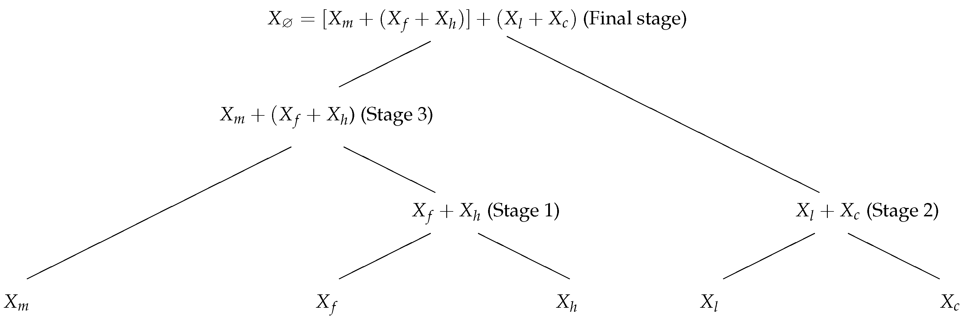
3.1. Tree Structure of the Hierarchical Copula Model

The first element of the hierarchical copula model is the rooted tree $\tau$ associated with random variables $X_i$, representing the loss ratios for individual business lines. As explained in Section 2.2 to build the tree we start by allocating the loss ratio of each business line to one leaf node and then aggregate the two random loss ratios, with the highest dependence measured by Kendall’s tau. Table 2 shows the Kendall’s tau estimates for the gross loss ratios of each pair of business lines. At each stage we aggregate the two loss ratio random variables with the strongest Kendall’s tau estimate.

After allocating each business line to a leaf node, as in the bottom row of the tree depicted in Figure 2, we aggregate the two business lines with the strongest dependence. From Table 2 we observe that House and Fire have the largest Kendall’s tau. Hence, at this first stage, we aggregate these two business lines. In stage 2, the largest Kendall’s tau observed is between CTP and Liability. We then aggregate CTP and Liability. In stage 3 the strongest dependence is between Motor and Fire + House, leading to the aggregate between them. In the fina stage, we aggregate together the two resulting loss ratios, namely Motor + Fire + House and Liability + CTP. This is illustrated in Figure 2.

Table 3 contains the Kendall tau values for the case of the net (after reinsurance) loss ratio for the five business lines. The variables more strongly dependent, at the different stages of the construction of the tree, are the same as for the gross loss ratios case. As a consequence the structure of the rooted tree for the net loss ratios hierarchical copula model is the same as for the gross loss ratios shown in Figure 2. In the last stage of the aggregation model the Kendall’s tau between the net loss ratios for House, Fire, Motor, CTP and Liability together is -0.0892.

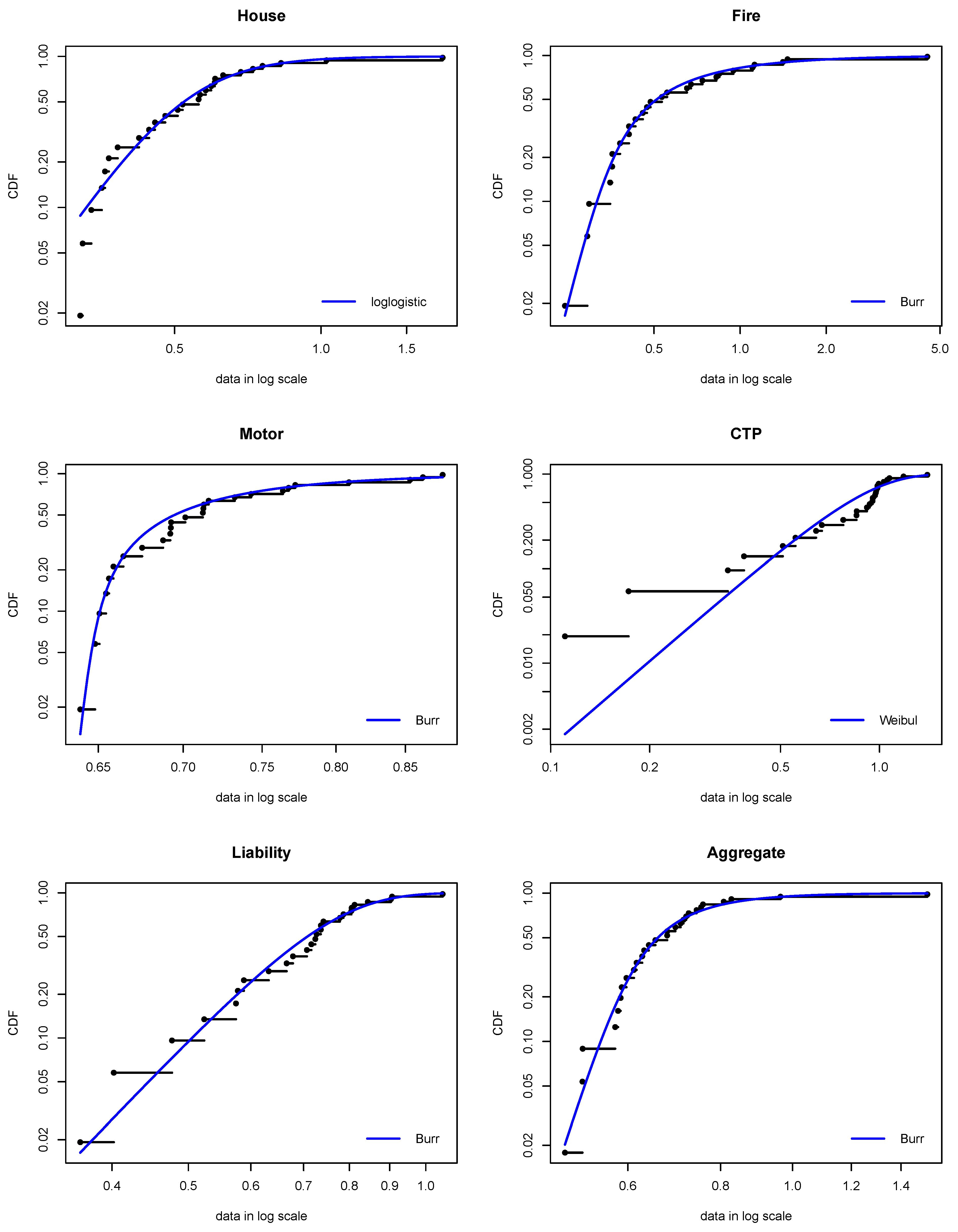
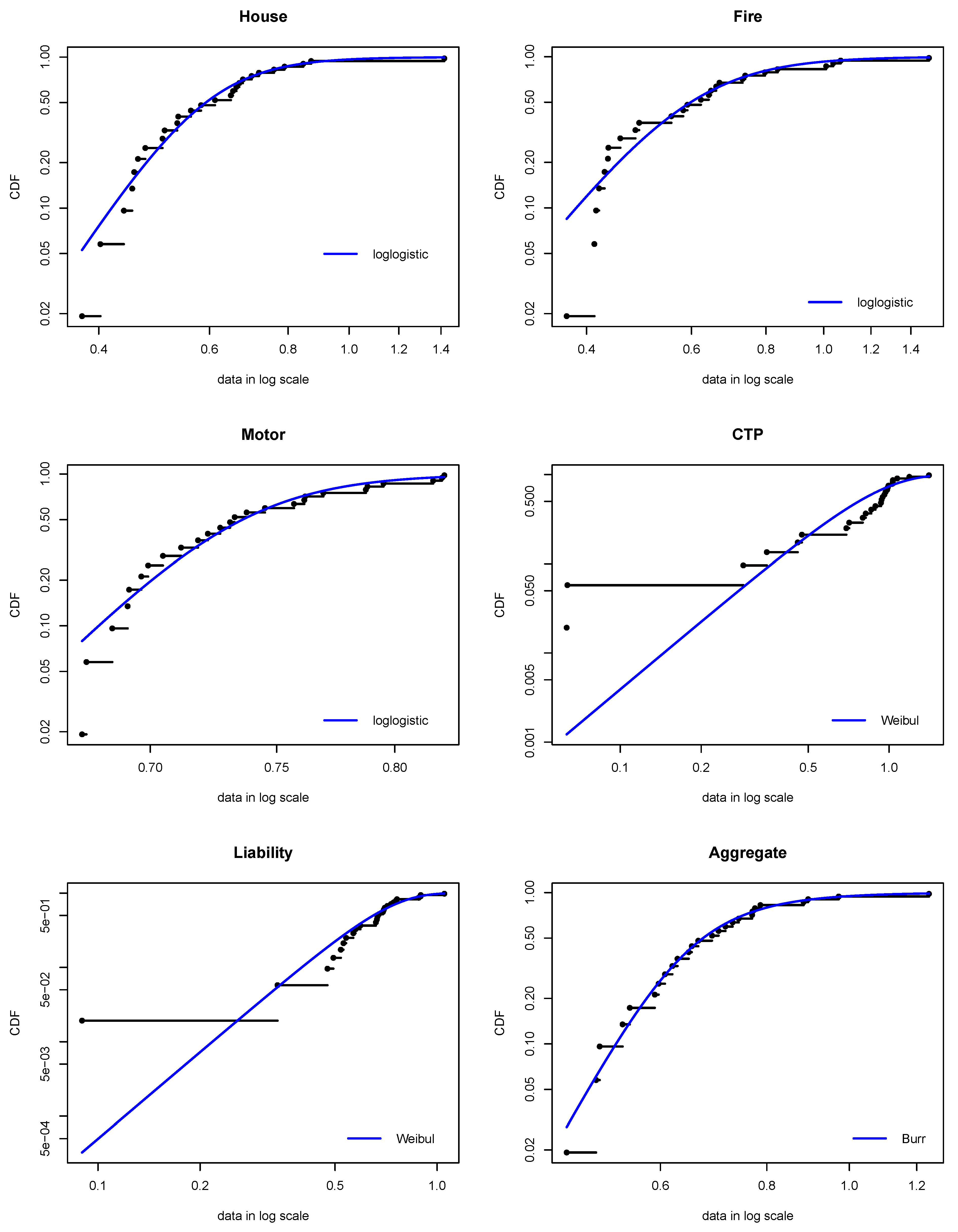
3.2. Fitting the Univariate Probability Distributions

Next, we will fit the probability distributions for individual loss ratios, based on the maximum likelihood estimation and Anderson and Darling (A-D) goodness of fit test. As we are primarily interested in estimating the measures of risk, which are based on the tail of the distributions, it is important to use an appropriate test. It is known that the A-D test is more powerful and sensitive to the tails of the distribution (see [23]) than other alternative tests such as the commonly used Kolmogorov-Smirnov5 goodness-of-fit test. Hence, we choose the distribution that produces the highest p-value according to the A-D test. For each business line we fit the following families of distributions: Lognormal, Gamma, Weibull, Loglogistic, Pareto and Burr. The results for the distribution with the highest A-D test p-value and corresponding parameter estimates are listed in Table 4. The fitted distributions for the loss ratios are log-logistic, Burr and Weibull distributions. These fitted distributions are also visualised in Figure 3 and Figure 4 for gross and net loss ratios, respectively.

3.3. Determining Joint Distribution Through Copulas

Having determined the best fit univariate distribution for each business loss ratio, we can estimate the joint distributions for each pair of loss ratios at each branching node in Figure 2, by coupling the corresponding univariate probability distributions. We consider the following commonly used copulas: Gaussian copula, the Student-t, the Frank, the Clayton, the Gumbel, the mixtures of Clayton and Gumbel copulas and corresponding survival copulas. The Gaussian copula is appropriate to model data with elliptical shape but does not allow for tail dependence between the business lines. The Student-t copula, although also elliptical, allows for tail dependence. The Frank copula is suitable to symmetric data and can perform better than the Gaussian copula in certain cases. The Clayton and the Gumbel copulas are used when data shows asymmetric tail dependence (lower or upper, respectively). Mixtures of Clayton and Gumbel, and survival copulas can potentially perform better when the data exhibits tail dependence in both tails, even if asymmetric.

We calculate and report in Table 5, the non-parametric estimates of the upper and lower tail dependence coefficients (see [41,43]) for each pair of loss ratios associated with the children of each branching node. As the risk of extreme events is one of the main concerns when it comes to capital requirements, it is important to pay particular attention to the tails of the copula distributions in the modelling process. Table 5 summarizes the results of the selected copulas for the four branching nodes for both gross and net loss ratios.

To select between copula models we use the goodness-of-fit test statistic $S_n$ from [26]. In the cases of the mixture models, to determine the weight of each copula family we fit a model with weight $\alpha$ for the first copula and $1-\alpha$ for the second copula, for a sequence of values $\alpha$ varying in $[0,1]$. We then choose the estimate $\widehat{\alpha }$ for the mixture that maximises the goodness-of-fit statistic. For the gross loss ratios the first node is Fire and House ($X_f$ + $X_h$), as shown in Figure 2. From Table 5 we can see that both lower (${\lambda }_L$) and upper (${\lambda }_U$) tail coefficient estimates are different from zero. The copula with the highest p-value is a mixture of $40\%$ Clayton and $60\%$ survival Clayton copulas. As the Clayton copula allows for tail dependence, and the estimates for the upper and lower tail dependence are slightly different, the mixture model seems to be a reasonable choice. The p-value of the $S_n$ goodness of fit test, the parameters and standard errors estimates are also listed Table 5. For the business lines CTP and Liability the best copula is a mixture of $25\%$ Clayton and $75\%$ survival Clayton copulas. The same copula mixture is again the best for Motor and Fire plus House but with only $10\%$ weight on the Clayton component of the mixture. The estimates for the tail coefficients for the two root node children, Motor plus Fire plus House and CTP plus Liability, are zero. Indeed the best copula, according to the goodness of fit test, is the Gaussian copula which has no tail dependence. This choice makes sense as the estimates for the upper and lower tail dependence are zero.

For the net loss ratios the best copula for the House and Fire pair is $60\%$ Gumbel plus $40\%$ survival Gumbel. The resulting copula has both upper and lower tail dependence witch is in line with the non-parametric estimates. CTP and Liability is best modelled by a Student-t which also allows for both upper and lower tail dependence. A mixture of $70\%$ survival Gumbel with $30\%$ survival Clayton has the higher p-value for Motor and Fire plus House. The estimate for the Kendall’s tau for the pair Motor plus Fire plus House and CTP plus Liability is close to zero but negative. Hence we flip the variable Motor plus Fire plus House after transforming it into the zero one interval. By flipping we mean subtract the variable from one. The best copula for the resulting pair is then a Gumbel copula which allows for tail dependence between low values of Motor plus House plus Fire and high values of CTP and Liability.

3.4. Simulation of the Aggregate Loss Ratios

In order to estimate VaR and TVaR from the hierarchical copula aggregation model we can now simulate observations of aggregate loss ratios using the model constructed in the previous sections. We implement the sample reordering algorithm from Section 2.2.2 for the gross and net loss ratios using $N=1000$. Using the estimator from equation (1) we estimate the TVaR for each business line, gross and net, loss ratios for the confidence levels of $90\%$, $95\%$ and $99\%$. The VaR estimate for a given confidence level is the corresponding empirical quantile. The results are presented in Table 6 and its analysis follows in the next sections.

3.4.1. Analysis of the Results

From Table 6 we can see that Fire has the largest VaR and TVaR among the five business lines for the gross loss ratios, followed by CTP except for the $99\%$ TVaR, where House has the second largest. When we consider reinsurance, by analysing the net loss ratios, CTP has the largest risk measure values while Fire has the second largest except for the $99\%$ TVaR where Fire still has the largest value. Nevertheless the $99\%$ TVaR for Fire has a staggering reduction after reinsurance. Overall Motor has the lowest values for the risk measures in terms of both gross and net loss ratios, implying the least risky business line. The VaR and TVaR 95% confidence intervals for gross and net losses overlap in the cases of House, CTP and Liability. For Fire, Motor and (copula) aggregate losses the confidence intervals for gross and net losses do not overlap. We conclude that reinsurance is effectively reducing the level of risk only for Fire and Motor. And this reduction is strong enough to carry on to the (copula) aggregate loss. The effect of reinsurance in changing the risk level for House, CTP and Liability is much less pronounced. We come back to this point later in this article. It is worthwhile recalling here that the average loss is also not significantly different with and without reinsurance.

Comparing the two right columns of Table 6 we can see that the weighted sum of the risk measures, VaR and TVaR, is larger than the value obtained using the hierarchical aggregation copula model. This is true both for VaR and TVaR at all the probability levels considered, and for gross and net loss ratios. The risk measures obtained using the hierarchical copula model incorporate the dependence between the different business lines while the weighted sum of VaR and TVaR does not. Hence, the result obtained is clear evidence that there is a risk reduction effect in the tails when combining the five business lines. This reduction of risk by pooling different business lines (risks) corresponds to the notion of diversification well known in financial portfolio selection and asset allocation.

4. The Effect of Reinsurance

Our goal now is to explore the effect of reinsurance on the diversification of the portfolio composed by the different business lines. Conceptually we are here drawing some parallel between a portfolio of financial assets and the set of business lines. When addressing diversification in terms of portfolio selection we can think of two aspects. First, diversification is affected by the weights of each component of the portfolio. Second, diversification can also be affected by the sources of risk and the interaction between the different business lines. We address these two cases below separately.

4.1. Reinsurance and Weighted Premiums Diversification

Here we evaluate the effect of reinsurance on the diversification due to changing the proportion of underwritten premiums (weights) for the different business lines. Insurance companies cede risk to the reinsurer in different proportions for the different business lines. As a result the weights of each business line, corresponding to the proportion of underwritten premiums, in the insurers portfolio before and after considering reinsurance are different. For the data analysed in this paper, the weights as of June 2017 are reported in Table 1, we can see that reinsurance reduces the proportion of the business lines of Fire and House, and increases the weight of Motor.

A measure of diversification which concentrates on the weights of each portfolio component is derived from the concept of Shannon’s entropy, introduced in [42] for information theory. Within a financial portfolio setting, Shannon’s entropy measures diversification as

$$H\left(w\right)=-\sum _{i=1}^N{w}_{i}ln{w}_i,$$

where ${\sum }_{i=1}^N{w}_i=1$, $w_i\ge 0$ and N is the number of portfolio components. According to this measure equal weights correspond to the highest diversification. The background idea is that equal weights correspond to maximum information. We refer to [20] for a study on the (superior) out-of-sample performance of an equally weighted financial portfolio.

The values obtained for the Shannon’s entropy measure for the insurance data are listed in Table 7. We find that the diversification of the portfolio considering reinsurance is lower than the diversification of the portfolio without reinsurance. The change in the weights between the business lines is largely due to the higher cession rate on Fire. We can see that there is a link here between a higher cession rate (mainly) on the business line Fire through reinsurance and a reduction in the diversification of the portfolio. The value for the Shannon’s entropy of an equally weighted portfolio is $1.61$. So the equally weighted portfolio is $6\%$ more diversified than the portfolio without reinsurance and $8\%$ more diversified than the portfolio after considering reinsurance.

4.2. Reinsurance and Source of Risk Diversification

One goal of diversification is to reduce the risk in the portfolio by taking advantage of the relation between the different components. One way of measuring portfolio diversification taking the sources of risk into account is by calculating the diversification ratio (DR) from [13]. This measure uses both the weights and the risk of each component of the portfolio producing a weighted average of the components risk. The expression for the diversification ratio is given by

$$DR={\displaystyle \frac{{\sum }_{i=1}^N{w}_i{\lambda }_i}{{\lambda }_P}},$$

where ${\sum }_{i=1}^N{w}_i=1$, $w_i\ge 0$, ${\lambda }_i$ is the risk of component i, and N is the number of portfolio components. In the denominator of the diversification ratio, ${\lambda }_P$ is the portfolio risk and hence the relation between the different components of the portfolio is taken into account by the diversification ratio. Using standard deviation, VaR and TVaR as measures of risk, we obtain the diversification ratio values. The VaR and TVaR risk measures for the weighted sum of business lines loss ratios are the ones obtained by the hierarchical aggregation copula model. The weights are fixed and based on the premiums as at June 2017. The results are reported in Table 8.

The results show that the diversification ratio increases with reinsurance, most strikingly when we use standard deviation as measure of risk, where the diversification ratio increases by $24\%$. This indicates that reinsurance increases diversification for the smaller more frequent claims to a larger extent than for the larger less frequent claims. For the VaR and TVaR the increase in diversification is modest, around $3\%$, with the exception of TVaR at the $99\%$ level to which reinsurance implies $12\%$ increase of the diversification ratio. This indicates that, from a multivariate or portfolio point of view, by reducing the high upper tail dependence of some of the loss ratios across the different business lines (the estimates for ${\lambda }_U$ in Table 5 do not contradict this assertion), reinsurance is increasing the diversification ratio. Considering the results from Shannon’s entropy measure, we conclude that although reinsurance is reducing the (weights) diversification, this is compensated by the reduction in risk producing higher diversification ratios. As far as we know these effects of reinsurance on the multivariate overall portfolio of business lines has not been previously found in the literature.

5. Conclusion

It is important for every insurance company to determine and maintain the right amount of capital to keep as a solvency margin against the risk of not being able of covering the insurance company’s liabilities. This calls for adequate methods of aggregating all risks and the use of appropriate risk measures to determine the capital requirement. In this article we use a hierarchical aggregation copula model to address the dependence structure of the different insurance business lines. We use several copula families to model the aggregated loss with particular emphasis on capturing the tail dependence. We consider a range of copulas asymmetric, symmetric, with and without tail dependence as the Gaussian and Student-t, and Archimedean copulas Clayton, Gumbel, and Frank. Selecting the best copula families for the hierarchical aggregation model is crucial as it influences the estimated level of risk and consequently avoids over or underestimation of the capital required. We must stress that this study looks for empirical evidence of the effect of reinsurance on a portfolio of insurance business lines. This means that the methodology used is very much tailored for the particular case and dataset used, and the following conclusions are constrained by our specific application. Our goal is to show, based on the data used, that there are important issues to be considered and show a possible roadmap for other cases.

A very important tool for risk management is reinsurance. Insurance companies diversify away part of its underwriting risk to reinsurance companies. In this paper we use the case of the Australian insurance market to investigate the effect and relevance of reinsurance on the risk of individual business lines and importantly on the aggregate risk. These effects are measured in this paper by considering both gross and net loss ratios, where gross loss ratios are used to measure the insurance risk without considering the reinsurance business, while the net loss ratios are used to determine the insurance risk taking into account reinsurance. For most business lines reinsurance reduces the risk, especially Fire and Motor, but it can also increase the risk even when measured by the standard deviation as we can see in Table 1 and Table 6 for the CTP and Liability business lines.

Another aspect of reinsurance pertains to diversification. By leveraging the interdependencies among various business lines, reinsurance enhances the diversification ratio, which takes into account both the weights and the source of risk. Conversely, it diminishes Shannon’s entropy diversification, which solely focuses on weights. Consequently, in the context of the Australian insurance market, we deduce that reinsurance can decrease the aggregate risk’s sensitivity to alterations in the proportions of different business lines. Therefore, if the objective is to manage risk by adjusting the proportion of underwriting among business lines, reinsurance may alleviate the decrease in aggregate risk. Hence, a comprehensive risk management strategy must encompass the three facets of weights, interdependencies among business lines, and reinsurance cession rates to effectively mitigate the aggregate risk in the insurance portfolio when the primary insurer transfers risk through reinsurance.

References

- Aas, K., Czado, C., Frigessi, A. and Bakken, H. 2009, `Pair-copula constructions of multiple dependence’, Insurance: Mathematics and Economics 44(2), 182 – 198.http://www.sciencedirect.com/science/article/pii/S0167668707000194. [CrossRef]
- Acerbi, C., Nordio, C. and Sirtori, C. 2001, `Expected shortfall as a tool for financial risk management’, arXiv preprint cond-mat/0102304.
- Acerbi, C. and Tasche, D. 2002, `On the coherence of expected shortfall’, Journal of Banking & Finance 26(7), 1487 – 1503.http://www.sciencedirect.com/science/article/pii/S0378426602002832.
- Adam, A., Houkari, M. and Laurent, J.-P. 2008, `Spectral risk measures and portfolio selection’, Journal of Banking & Finance 32(9), 1870 – 1882.http://www.sciencedirect.com/science/article/pii/S0378426608000101.
- Anderson, T. W. and Darling, D. A. 1954, `A test of goodness of fit’, Journal of the American Statistical Association 49(268), 765–769.
- Arbenz, P., Hummel, C. and Mainik, G. 2012, `Copula based hierarchical risk aggregation through sample reordering’, Insurance: Mathematics and Economics 51(1), 122–133.
- Bargès, M., Cossette, H. and Marceau, E. 2009, `Tvar-based capital allocation with copulas’, Insurance: Mathematics and Economics 45(3), 348–361.
- Baur, P., Breutel-O’Donoghue, A. and Hess, T. 2004, Understanding reinsurance: How reinsurers create value and manage risk, Swiss Re, Swiss Reinsurance Company.
- Becker, B., Opp, M. M. and Saidi, F. 2022, `Regulatory forbearance in the us insurance industry: The effects of removing capital requirements for an asset class’, The Review of Financial Studies 35(12), 5438–5482.
- Brechmann, E. C. 2014, `Hierarchical Kendall copulas: Properties and inference’, The Canadian Journal of Statistics 42(1), 78–108.
- Bürgi, R., Dacorogna, M. M. and Iles, R. 2008, `Risk aggregation, dependence structure and diversification benefit’, Stress Testing for Financial Institutions. [CrossRef]
- Chaoubi, I., Cossette, H., Marceau, E. and Robert, C. Y. 2021, `Hierarchical copulas with archimedean blocks and asymmetric between-block pairs’, Computational Statistics & Data Analysis 154, 107071.https://www.sciencedirect.com/science/article/pii/S0167947320301626.
- Choueifaty, Y. and Coignard, Y. 2008, `Toward maximum diversification’, Journal of Portfolio Management 35(1), 4051.
- Cipra, T. 2010, Financial and Insurance Formulas, Physica-Verlag.
- Clemente, G. P., Savelli, N. and Zappa, D. 2015, `The impact of reinsurance strategies on capital requirements for premium risk in insurance’, Risks 3(2), 164–182.
- Cossette, H., Gadoury, S.-P., Marceau, É. and Mtalai, I. 2017, `Hierarchical archimedean copulas through multivariate compound distributions’, Insurance: Mathematics and Economics 76(Supplement C), 1 – 13.http://www.sciencedirect.com/science/article/pii/S0167668716304553. [CrossRef]
- Côté, M.-P. and Genest, C. 2015, `A copula-based risk aggregation model’, The Canadian Journal of Statistics 43(1), 60–81.
- Cummins, J. D., Dionne, G., Gagné, R. and Nouira, A. 2008, `The costs and benefits of reinsurance’. Available at SSRN: https://ssrn.com/abstract=1142954.
- Czado, C. 2019, Analyzing Dependent Data with Vine Copulas: a practical guide with R, Lecture Notes in Statistics, 222, Springer.
- DeMiguel, V., Garlappi, L. and Uppal, R. 2009, `Optimal versus naive diversification: How inefficient is the 1/n portfolio strategy?’, The Review of Financial Studies 22(5), 1915–1953.
- Diestel, R. 2017, Graph Theory, 5th edn, Springer, Heidelberg.
- Embrechts, P., Lindskog, F. and McNeil, A. 2003, Modelling dependence with copulas and application to risk management, in S. Rachev, ed., `Handbook of Heavy Tailed Distributions in Finance’, Elsevier, chapter 8, pp. 329–384.
- Engmann, S. and Cousineau, D. 2011, `Comparing distributions: the two-sample Anderson-Darling test as an alternative to the Kolmogorov-Smirnoff test’, Journal of Applied Quantitative Methods 6(3), 1–17.
- Floreani, A. 2013, `Risk measures and capital requirements: a critique of the solvency ii approach’, The Geneva Papers on Risk and Insurance Issues and Practice 38(2), 189–212.
- Genest, C. and Nešlehová, J. 2012, `Copulas and copula models’, In:Encyclopedia of Environmetrics, 2nd ed., vol. 2, A.H. El-Shaarawi and W.W. Piegorsch, editors. Wiley, Chichester pp. 541–553. [CrossRef]
- Genest, C., Rémillard, B. and Beaudoin, D. 2009, `Goodness-of-fit tests for copulas: A review and a power study’, Insurance: Mathematics and economics 44(2), 199–214.
- Giuzio, M., Krušec, D., Levels, A., Melo, A. S., Mikkonen, K. and Radulova, P. 2019, `Climate change and financial stability’, Financial Stability Review 1.
- Haff, I. H., Aas, K. and Frigessi, A. 2010, `On the simplified pair-copula construction—simply useful or too simplistic?’, Journal of Multivariate Analysis 101(5), 1296–1310.
- Iman, R. and Conover, W. 1982, `A distribution-free approach to including rank correlation among input variables’, Communications in Statistics - Simulation and Computation 11(3), 311–334.
- Joe, H. 1996, `Families of m-variate distributions with given margins and m(m-1)/2 bivariate dependence parameters’, Lecture Notes-Monograph Series 28, 120–141.http://www.jstor.org/stable/4355888.
- Kolmogorov, A. 1933, `Sulla determinazione empirica di una lgge di distribuzione’, Inst. Ital. Attuari, Giorn. 4, 83–91.
- Kurowicka, D. and Joe, H. 2010, Dependence Modeling. Vine Copula Handbook, World Scientific, Singapore.
- Li, P. and Yin, C. 2024, `The tail mean–variance optimal capital allocation under the extended skew-elliptical distribution’, Journal of Computational and Applied Mathematics 448, 115965.
- Mai, J.-F. and Scherer, M. 2012, `H-extendible copulas’, Journal of Multivariate Analysis 110(Supplement C), 151 – 160. Special Issue on Copula Modeling and Dependence.http://www.sciencedirect.com/science/article/pii/S0047259X12000802. [CrossRef]
- McNeil, A. J., Frey, R. and Embrechts, P. 2015, Quantitative Risk Management: Concepts, Techniques and Tools, second edn, Princeton University Press, Princeton, NJ.
- MunichRe 2010, `A basic guide to facultative and treaty reinsurance.’, Munich Reinsurance America.
- Nanthakumar, A. 2022, `A comparison of vine and hierarchical copulas as discriminants’, International Journal of Statistics and Probability 11(4), 13–24.
- Nelsen, R. B. 2006, An Introduction to Copulas, second edn, Springer-Verlag, New York.
- Nguyen, T., Molinari, R. D. et al. 2011, `Risk aggregation by using copulas in internal models’, Journal of Mathematical Finance 1(03), 50.
- OECD 2017, `International comparisons.’, OECD Insurance Statistics 2016, OECD Publishing, Paris. pp. 45–79.
- Schmid, F. and Schmidt, R. 2007, `Multivariate conditional versions of spearman’s rho and related measures of tail dependence’, Journal of Multivariate Analysis 98, 1123–1140.
- Shannon, C. 1948, `A mathematical theory of communication’, The Bell System Technical Journal 27(3), 379–423.
- Sibuya, M. 1960, `Bivariate extreme statistics’, Annals of the Institute of Statistical Mathematics 11(3), 195–210.
- Sklar, A. 1959, `Fonctions de répartition à n dimensions et leurs marges’, Publ. Inst. Statist. Univ. Paris 8, 229–31.
- Smirnov, N. 1948, `Table for estimating the goodness of fit of empirical distributions’, Annals of Mathematical Statistics 19, 279–281.
- Tang, A. and Valdez, E. A. 2006, `Economic capital and the aggregation of risks using copulas’, Proceedings of the 28th International Congress of Actuaries, Paris, France. Available at:http://www.ica2006.com/282.html.
- Taylor, J. M. 1997, Claim Reserving Manual, 1997 rev. edn, Faculty and Institute of Actuaries, Great Britain.
- Torri, G., Radi, D. and Dvořáčková, H. 2022, `Catastrophic and systemic risk in the non-life insurance sector: A micro-structural contagion approach’, Finance Research Letters 47, 102718. [CrossRef]
- Wang, S. 1998, Aggregation of correlated risk portfolios: models and algorithms, in `Proceedings of the Casualty Actuarial society’, Vol. 85, pp. 848–939.