

Submitted:
08 October 2024
Posted:
09 October 2024
You are already at the latest version
Abstract
With escalating global environmental challenges and worsening air quality, there is an urgent need for enhanced environmental monitoring capabilities. Low-cost sensor networks are emerging as a vital solution, enabling widespread and affordable deployment at fine spatial resolutions. In this context, machine learning for the calibration of low-cost sensors is particularly valuable. However, traditional machine learning models often lack interpretability and generalizability when applied to complex, dynamic environmental data. To address this, we propose a causal feature selection approach based on convergent cross-mapping within the machine learning pipeline to build more robustly calibrated sensor networks. This approach is applied in the calibration of low-cost optical particle counters, effectively reproducing the measurements of PM1 and PM2.5 as recorded by research grade spectrometers. We evaluated the predictive performance and generalizability of these causally optimized models, observing improvements in both while reducing the number of input features, thus adhering to the Occam’s razor principle. For the PM1 calibration model, the proposed feature selection reduced the mean squared error on the test set by 43.2% compared to the model with all input features, while the SHAP value-based selection only achieved a reduction of 29.6%. Similarly, for the PM2.5 model, the proposed feature selection led to a 33.2% reduction in the mean squared error, outperforming the 30.2% reduction achieved by SHAP value-based selection. By integrating sensors with advanced machine learning techniques, this approach advances urban air quality monitoring, fostering a deeper scientific understanding of microenvironments. Beyond the current test cases, this feature selection method holds potential for broader application in other environmental monitoring applications, contributing to the development of interpretable and robust environmental models.
Keywords:
machine learning
; causality
; sensor calibration
1. Introduction
The human quality of life is intricately intertwined with the physical environment surrounding us. We are now experiencing an era marked by unprecedented, widespread, and intense changes in the global environmental state [1]. Driven by human activities and population growth, significant global warming and consequent climate change are disrupting the usual balance of nature, posing a fundamental threat to various aspects of life. Human health is particularly affected, most significantly through its relationship with air quality. Global change and air quality are intertwined [2,3], and air quality is intricately related to human health. Air pollution is one of the greatest environmental risks to health. The World Health Organization (WHO) estimates that 4.2 million deaths annually can be attributed to air pollution [4]. Poor air quality due to pollutants such as ozone, particulate matter (PM), and sulfur dioxide can lead to a variety of health problems, including asthma, heart disease, and lung cancer. Associations have been reported between the concentrations of various air pollutants and diabetes, mumps, and epilepsy [5]. While the effects of climate change on air quality vary by region, many areas suffer a decline in air quality in parallel with global environmental change. Shifting weather patterns, including changes in temperature and precipitation, is expected to raise levels of PM. Robust evidence from models and observations shows that climate change is worsening ozone pollution. Climate change is expected to affect indoor heating and cooling demand due to temperature changes, altering fuel use, and consequently the composition of the emitted air pollutants. Evidence suggests that without additional air pollution controls, climate change will increase the risk of poor air quality in the US. [6]. Therefore, the current state of global change and the concurrent exacerbation of air quality degradation emphasize the need for enhanced environmental monitoring capabilities at appropriate spatial scales.
Internet of Things (IoT) has proved pivotal in this respect, enabling real-time data collection with high spatio-temporal resolution through networks of interconnected sensors. However, accessible, wide-scale deployment for environmental monitoring at more localized scales requires low-cost air quality sensor systems (LCS) [7]. Although LCS have the potential to bridge the gaps in sensor networks, thus facilitating dense monitoring networks capturing the relevant spatial variations of pollutants, they are less precise and have several sources of greater uncertainty compared to research-grade monitors. They are also more sensitive to environmental conditions. This makes them more likely to introduce potential measurement discrepancies compared to their reference sensors [8,9]. Therefore, LCS require calibration prior to field deployment in order to improve the reliability and accuracy of the data being collected. This process involves the collocation of the LCS alongside a reference monitor at a representative location/s and then using the collected data to develop a calibration model that maps the raw output of the LCS to the measurements from the reference monitor. While several calibration mechanisms exist, machine learning is gaining popularity as a leading approach to LCS calibration [10,11,12].
1.1. Machine Learning and the Need for Causality
Machine learning (ML) is a subset of artificial intelligence. It involves creating algorithms and statistical models that allow computers to learn from data and make predictions without the need for explicit programming. That is, learning through examples. ML has now gained immense popularity, and almost all sectors in the industrial arena leverage machine learning solutions to enhance productivity, decision-making processes, and other aspects [13,14,15,16].
It has proved useful in a wide variety of applications in science and engineering as well, especially for those applications where we do not have a complete theory, yet which are of significance. Particularly in the field of Atmospheric Science and Climate Physics, ML techniques are being used as an automated approach to build empirical models from data alone [17,18,19].
Despite their wide usage and relative success, most traditional ML methodologies are constrained in their performance due to inherent limitations. One such limitation is the lack of interpretability [20,21,22]. Although adept at extracting patterns from data, ML systems develop complex models with numerous inputs that are often challenging to interpret. These models typically function as opaque black boxes, lacking the capability to elucidate the rationale behind their predictions or recommendations, or why a specific feature is prioritized compared to others in a model. Although model interpretation techniques such as SHAP values [23] are beneficial, they offer information solely on the functioning of the model that was learned, but not necessarily on how the variables under consideration relate to each other in the physical world. Empirical risk minimization commonly practiced in ML is designed to minimize a loss function on observed data, aimed at optimizing some performance metric. This approach is suboptimal since blindly optimizing for the performance on a finite dataset runs the risk of prioritizing associations within the dataset rather than actual cause and effect instances, thus leading to an incomplete problem formulation. In most scientific applications where we may seek to empirically model a phenomenon being studied, or where decisions are being made based on predictions from a ML model, and therefore unfavorable results have significant implications, interpretable ML models are essential. This is to foster not only scientific understanding and justification for model predictions, but also safety and reliability, since fully testing an end-to-end system, exhaustively anticipating every potential scenario where the system could fail, is not feasible for most complex tasks. In such cases, the incompleteness associated with the absence of sufficient interpretability can lead to unquantified bias [21]. This is one motivation for ensuring that feature-target pairs utilized by a ML model reflect genuine causal relationships in the real world and not mere statistical correlations present within a finite dataset. This closely ties to the other drawback, which is a lack of robustness or generalizability. That is the ability to be deployed in a different environment or domain than the one in which it was trained, and yield as good a performance [24,25,26]. In supervised learning, the objective is to predict unknowns using available information by learning a mapping between a set of inputs and corresponding outputs. If due caution is not exercised, there is a risk of overfitting, where the algorithm fits too closely or even exactly to its training data. An overfit model would have learned and potentially prioritized the spurious correlations present within the dataset, specific to that particular distribution of data. Once the prediction environment diverges from the training environment, performance degradation should be anticipated since the model has learned to rely on superficial features that are no longer present. This is due to variations in the feature-target correlations between different environments. Determining whether the data generation process at the prediction time matches the training time is often uncertain, especially once deployed. In this vein, there are several studies in the literature that cite instances where ML models prioritize feature-target correlations specific to the datasets they have seen, and consequently generalize poorly to new unseen data [27,28,29]. ML models are by nature sensitive to spurious correlations [28]. Models relying on spurious correlations that do not always hold for minority groups can cause the model to fail when the data distribution is shifted in real-world applications. This is especially concerning for machine learning applications involving atmospheric and other environmental data, as is the case in LCS calibration for environmental monitoring, since the dynamic nature of the data renders it constantly shifting, sometimes even abruptly reaching extremes. This makes it virtually impossible to assert with certainty that the training data perfectly align with real-world instances once the model is deployed in the long term. Hence, in order to ensure that predictions made by ML models outside of the immediate domain of the training dataset remain accurate, we need models that are invariant to distributional shifts. That is, a model that would have learned a mapping which does not prioritize mere correlations, but rather features that affect the target in all environments. This need for invariance in ML models is another motivation for integrating causality into ML pipelines. This is because causal relationships are invariant. Mere correlation does not imply causation. If two variables are causally related, it should remain consistent across all environments. The invariance of causal variables is well established in the literature [30,31,32]. Consequently, a model making predictions exclusively using features directly causally related to the target should be more robust compared to general models.
Hence, in this study, we propose a feature selection step within our ML pipeline, based on causality, suitable for complex systems. The objective is to select a subset of relevant features from a larger set of available features based on causal relationship to the target. Feature selection is a crucial step in developing machine learning models, aligning with the principle of Occam’s Razor, which favors simpler hypotheses. Most conventional feature selection approaches employ filter methods where features are ranked or scored based on measures such as SHAP or LIME values [33], with a threshold applied to select the top ranked features. However, if the model has learned and relies on spurious correlations, the feature importance derived from these methods will also reflect those spurious relationships. Consequently, relying on potentially misleading feature explanations compromises the generalizability we aim to achieve in our LCS calibration models. Another widely used approach is to rank features based on mutual information with the target variable. This is inadequate, as mutual information captures general statistical dependence rather than causal relationships. By adopting a causal approach to balance simplicity and predictive accuracy, we aim to leverage the well-established invariance of causal variables, enabling the development of more robust, accurate, and interpretable calibration models.
The study is structured as follows: In Section 2, we outline the proposed methodology for feature selection, detailing the underlying principles and techniques employed. This methodology is then applied to two case studies: calibration of a low-cost optical particle counter to reproduce PM1 and PM2.5 measurements from a research grade sensor. For comparison, we also develop calibration models for both case studies using two alternative approaches: (1) with all available features as predictors and (2) feature selection based on SHAP values. Section 3 presents the results, comparing the performance of the three approaches across the two case studies.
2. Materials and Methods
We first briefly outline the principle of convergent cross mapping (CCM), as developed in [34] and elaborated in [35], which forms the backbone of the proposed feature selection mechanism. CCM is a method that can distinguish causality from correlation that is based on nonlinear state space reconstruction. This approach is specifically designed for nonlinear dynamics, which are predominant in nature and exhibit deterministic characteristics. Deterministic systems differ from stochastic ones primarily in terms of separability. In purely stochastic systems, the effects of causal variables are separable—meaning that information associated with a causal factor is unique to that variable and can be excluded by removing it from the model. This implies that stochastic systems can be understood in parts rather than as an integrated whole. This does not hold true for most complex dynamic systems such as climate systems, ecological systems, biological systems etc., which do not satisfy separability. Therefore CCM provides a more rigorous and overarching causal mechanism more suited for the complex dynamics of the datasets commonly dealt with in machine learning problems, especially in environmental sciences.
CCM is based on the principle that if a system possesses deterministic aspects and its dynamics are not entirely random, then there exists a structured manifold that governs these dynamics, exhibiting coherent trajectories. In dynamical systems theory, two time-series variables, X and Y, are causally linked if they are coupled and part of the same underlying dynamic system, which is represented by a shared attractor manifold, M. In such a case, each variable contains information about the other. If X influences Y, then Y holds information that can be used to recover the states of X. CCM measures causality by determining how well the historical states of Y can estimate the states of X, which would only be possible if X causally influences Y.
Takens’ theorem [36] provides the theoretical foundation for this approach, stating that the essential information of a multidimensional dynamic system is preserved in the time series of any single variable. Therefore, a time series of one variable can be used to reconstruct the state space of the system. When X causally influences Y, the dynamics of the system can be represented by the shadow manifolds and , constructed from the lagged values of X and Y, respectively. These shadow manifolds will map onto each other since X and Y should belong to the same dynamic system. Nearby points on should correspond to nearby points on , indicating a causal relationship. If so, Y can be used to estimate X, and vice versa. The degree to which Y can be used to estimate X is quantified by the correlation coefficient between the predicted and observed values of X, a process referred to as cross mapping. As the length of the time series increases, the shadow manifolds become denser, improving the precision of cross mapping—a phenomenon known as convergent cross mapping, which is the key criterion for establishing causality. The convergence property is crucial for distinguishing true causation from mere correlation. The degree to which the predictive skill converges can be interpreted as an estimate of the strength of the causal relationship.
As detailed in [34], CCM is distinct from other cross-prediction methods, as it focuses on estimating the states of one variable from another, rather than forecasting the future states of the system. This distinction is particularly important in systems with chaotic dynamics, where prediction can be hampered by phenomena such as Lyapunov divergence. CCM also handles non-dynamic, random variables, making it a robust tool for causality detection in complex systems.
2.1. Proposed Feature Selection Mechanism
We now elaborate our novel feature selection scheme. It is important to note that there may be other causally-inspired feature selection methods in the literature. An example would be the automatic feature selection method for developing data-driven soft sensors in industrial processes proposed in [37]. This approach asserts that the capacity of a feature to reduce the uncertainty of a target variable, as measured by Shannon entropy, quantifies the causal impact of that feature on the target. Our approach is not intended to compete with such methods; rather, ours is designed specifically to handle the complexity of environmental and climate data. While information theory and entropy-based causal inference methods might be well suited for random variables, for atmospheric and environmental variables exhibiting complex interplay between various factors, CCM provides comparatively more solid criteria for causation, rigorously rooted in dynamical systems theory. The more generalized approach of CCM is more compatible with atmospheric and climate data that possess both stochastic as well as deterministic aspects, and due to its ability to identify weakly coupled interactions, which can play a significant role in complex systems where components influence each other, but do not directly cause drastic changes, or exhibit intricate feedback relations, we deem this a more suitable causal approach for the type of intricate systems addressed in environmental monitoring [35,38,39,40].
Hence, we propose a feature selection process for machine learning in which we leverage the principle of causation as imposed by CCM. Given a set of features (in the case of LCS calibration, these would be individual output measurements from the LCS along with external parameters such as ambient atmospheric pressure, temperature and humidity to account for the sensitivity to environmental conditions) with the target variable Y (the target variable as measured by the reference instrument), our proposed work flow is as follows.
- 1:
-
For each in , the causation criteria set by CCM for is evaluated. For the current study, the causal-ccm package [41] was used for this purpose.In evaluating the causal relationship from to Y, it is essential to select a sufficiently long time series for both variables in order to ascertain that the criterion of convergence is met and that the cross-map skill does not deteriorate significantly over time.
- 2:
- 3:
- Next, the remaining features are ranked according to the strength of the causal relationship , from most causally related to Y to the least.
- 4:
-
An appropriate threshold value is established for the strength of causality and the features exceeding this threshold are selected. The machine learning models are then constructed and trained for all possible subsets of the selected features as input variables to the model. After training, for each instance, the efficacy is tested using an independent validation data set to assess how well it performs when presented with data that the algorithm has not previously seen; i.e., test its generalizability.By exploring various subsets of the most causally related features, as opposed to simply selecting the top-ranked ones, we aim to refine the selection process to retain to the most possible extent only the most direct causal influences. This approach seeks to enhance the generalizability of models by utilizing direct causal parents for predictions, as discussed in studies such as [31].A reasonable choice of threshold for most cases would be , since any feature with a retained for an appropriate duration of time would have established a causation guaranteed above chance and thus beyond being wholly attributed to noise, systematic error, or biases in the observational data. However, depending on the complexity of the system being modelled, the threshold may need to be adjusted to accommodate features with comparatively lower values representing weak couplings that might offer important information to the model. Especially in climate systems, weakly coupled interactions are ubiquitous. An example of weakly coupled interactions can be found in the relationship between soil moisture and precipitation patterns. While soil moisture levels can influence local precipitation through mechanisms like evapotranspiration and land-atmosphere interactions, the coupling between soil moisture and precipitation is often not straightforward. However, understanding these weakly coupled interactions is crucial for accurate hydrological and climate modeling. By incorporating the nuanced effects of soil moisture on precipitation, models can better simulate regional water cycles, drought patterns, and the impacts of land surface changes on local climate conditions.
- 5:
- The model that demonstrates the best predictive performance is selected as the final calibration model. Performance metrics are compared with the full model to assess any improvement in generalizability. If no improvement is observed, the process in Step 4 is repeated using a lower threshold.
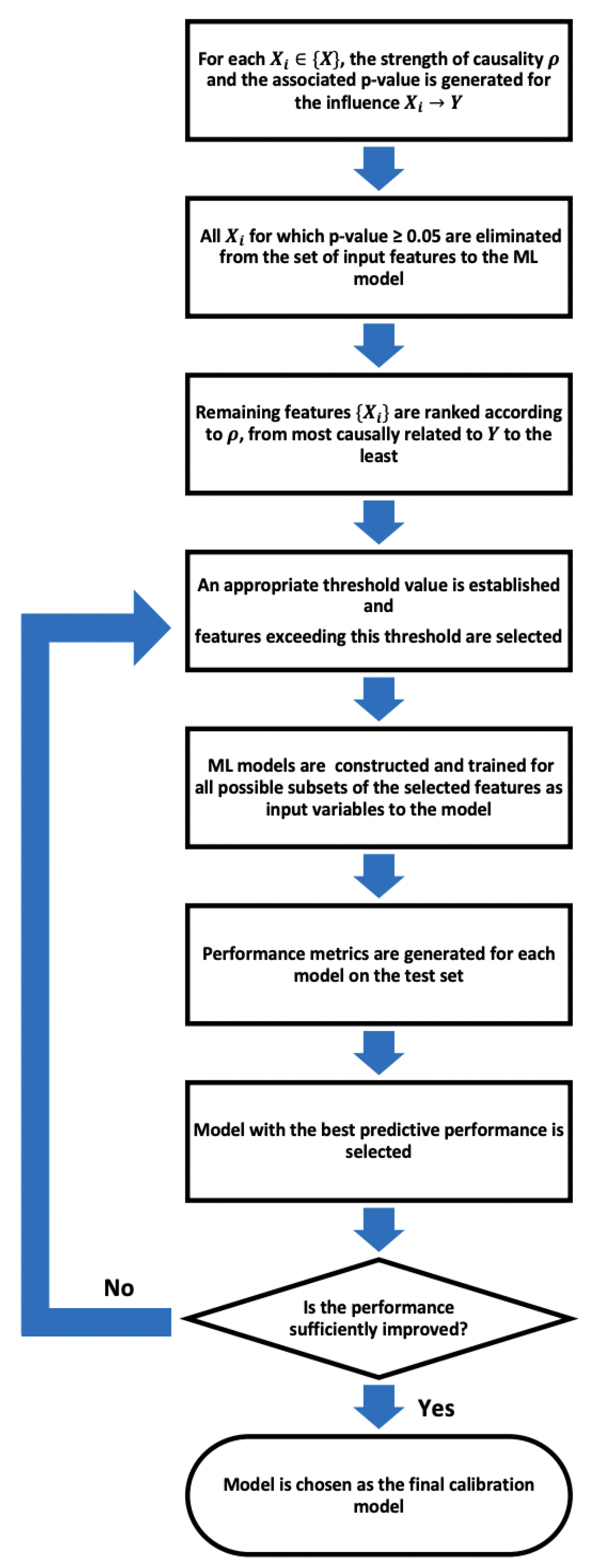
The Figure 1 gives a concise representation of the proposed feature selection.
2.2. Experimental Test Cases
In order to validate the proposed feature selection method, it was applied on two real-world LCS calibration instances.
2.2.1. Experimental Setup and Datasets Used
The two test instances were the calibration of a low cost optical particle counter (OPC) to reproduce the PM1 and PM2.5 counts from a research grade OPC.
The dataset was obtained from a previous study in [10]. The low-cost OPC used is a readily available, but much less accurate Alpha Sense OPC-N3 (http://www.alphasense.com/), together with cheaper environmental sensor (Bosch BME280). The OPC-N3 uses similar technology to the conventional OPCs where particle size is determined via a calibration based on Mie scattering. It is capable of on-board data logging and measuring particulates with diameters up to 40 , with a lower sensing diameter of 0.35 . The on-board data is saved within an SD card which can be accessed through micro-USB cable connected to the OPC. The OPC-N3 calculates its PM values using the method defined by the European Standard EN 481 [44].
The research grade reference OPC used is a GRIMM Laser Aerosol Spectrometer and Dust Monitor Model 1.109 (Germany). The sensor is capable of measuring particulates of diameters between 0.25 and 32 distributed within 32 size channels. Particulates entering the sensor are detected by scattering a 655 laser beam through a light trap. The sensor operates at a flow rate of 1.21 , classifying particles by size based on light intensity [45]. A curved optical mirror, positioned at a 90°scattering angle, redirects scattered light to a photo sensor, with its wide angle (120°) enhancing the light collection and reducing the minimum detectable particle size. It also compensates for Mie Scattering undulations caused by monochromatic illumination.
The data had been collected by collocating the LCS and the reference sensor unit at a field calibration station in an ambient environment from 02/12/2019 to 04/10/2019. There were in total 42 initial input features to our ML model, which included the particle counts for each of the 24 size bins measured by the OPC-N3; the OPC-N3 estimates of PM1, PM2.5, and PM10; a collection of OPC performance metrics, including the reject ratio, in-chamber temperature and humidity; and the ambient atmospheric pressure, temperature, and humidity from the BME280. The target outputs for estimation were the PM1 and PM2.5 abundance as measured by the reference instrument, each with its own empirical model. The data were first resampled at a frequency of 60 seconds, and the different data sources merged by matching the time.
Figure 1.
Proposed causality-driven feature selection pipeline.
We resampled the data for several key reasons. First, to ensure an evenly sampled time series for causal analysis using CCM, which relies on time-delay embeddings. Second, since this study involves constructing and training several benchmark models for comparison, a compact dataset was necessary to minimize computational time. A resampling frequency of 60 seconds was chosen to create a compact dataset without undersampling, while still adequately capturing temporal variability in PM levels. Finally, instances with missing values (NaN) were dropped from the dataset.
The genre of ML used was multivariate nonlinear nonparametric regression. According to [10], the best suited class of regression algorithms for the task is an ensemble of decision trees with hyper-parameter optimization. Therefore, the GradientBoostingRegressor implementation of Python 3.10 was used for ML tasks. Of the final cleaned and data-matched dataset, 2,130 data instances were isolated for hyperparameter optimization using cross-validation, a subset of which; a continuous time series of 600 time steps, was used for the causal feature ranking. The remaining dataset, consisting of 31,361 instances, was randomly partitioned into 80% for training and 20% for testing. To ensure the rigor of the process, there was no overlap between the training and testing datasets and the data used for causal analysis.
Separate calibration models were developed for each of PM1 and PM2.5. For each case, 3 approaches were employed and the results compared: a) Using all 42 variables from the LCS as input features to the ML model b) Using feature selection based on SHAP values c) Using the proposed causality-based feature selection.
PM1
First, all 42 output variables from the LCS described in Section 2.2.1 were used as input features with PM1 count from the reference sensor as the target variable for the ML model. The hyperparameters: the number of estimators (n_estimators), the learning rate (learning_rate), the maximum depth of the trees (max_depth), the minimum number of samples required to be at a leaf node (min_samples_leaf) and the number of features considered for splitting (max_features) were optimized using the GridSearchCV function of Python 3.10. The optimized model was then trained on the training dataset and applied on the independent test dataset and the performance of the model was assessed using mean squared error (MSE) and the coefficient of determination (R²), two widely employed performance evaluation metrics in ML.
The SHAP values were then generated on the training dataset for the model to assess the model-specific contribution of each feature in predicting the PM1 count, and the features were ranked according to importance. A commonly used threshold for SHAP value-based feature selection is 0.5, indicating a significant influence on predictions. However, in our case, that would have eliminated most features (Figure 2) leading to underfitting. Therefore, for a fair comparison with the causality-based feature selection, the 10 highest-ranked features (highlighted in red in Figure 2) were chosen. ML models were then constructed with hyperparameter optimization and trained for all possible subsets of the selected features as inputs. Each instance was applied on the independent test dataset, and the performance metrics were generated. The best model was selected based on the MSE on the test set.
Next, the causality-based feature selection described in Section 2.1 was applied with threshold . A higher threshold of 0.7 was selected in this case because mapping LCS readings to reference-grade measurements is a relatively straightforward task, making it less likely that weakly coupled variables would have significant effects. Therefore, as an initial attempt, we used a threshold of 0.7 to include the top 10 highest-ranked features (Figure 3). Then the best model was selected based on the MSE on the test set. For the time-delay embedding for CCM, since the time series were not overly sampled in time, the lag () was set to 1. The optimal embedding dimension (E) was empirically determined by applying simplex projection to the time series of the target PM1 counts from the reference sensor[40,46].
PM2.5
The same procedure was followed for the estimation of PM2.5 particle counts, now with the PM2.5 count from the reference sensor as the target variable.
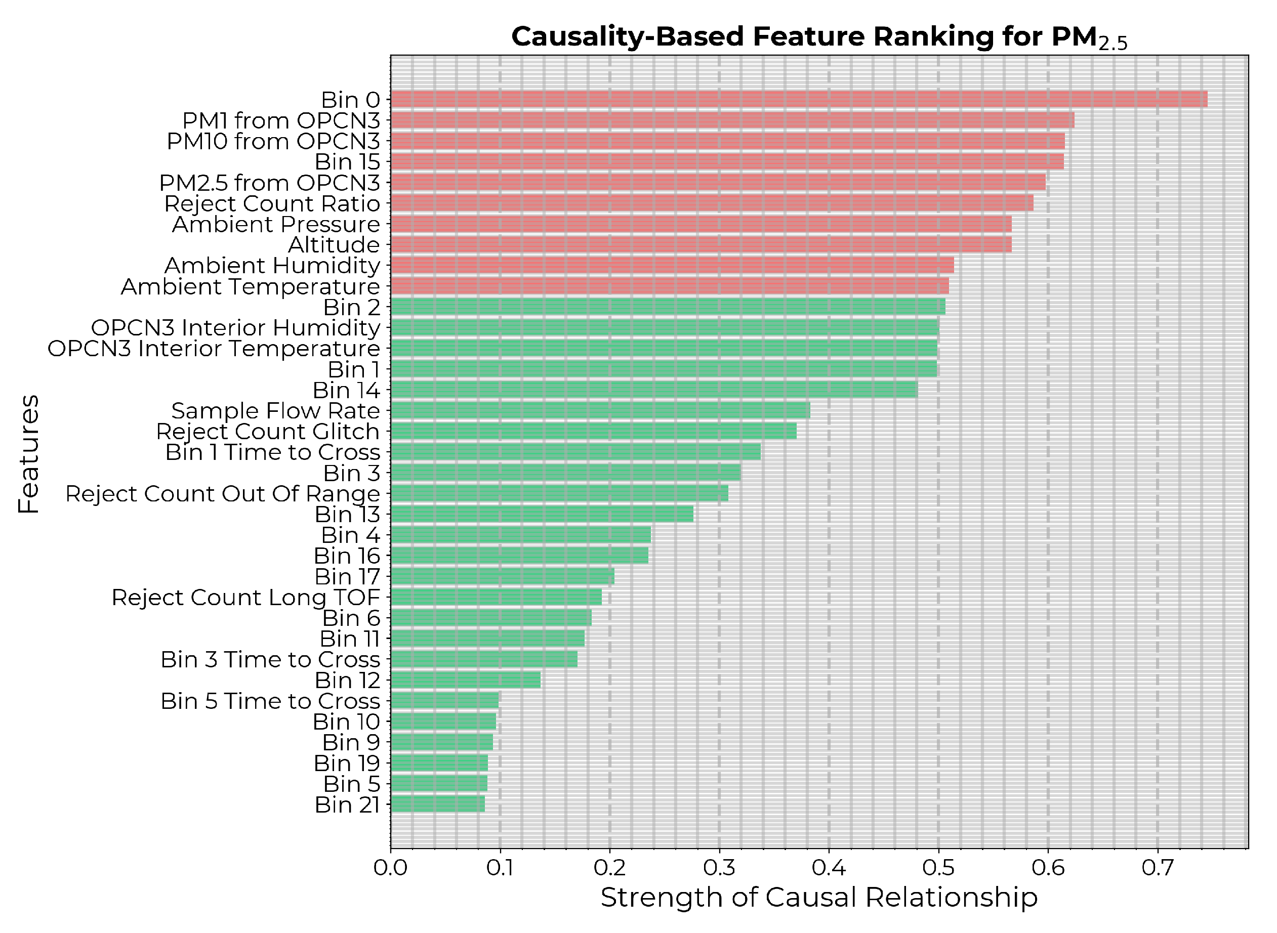
The feature importance ranking based on SHAP values is depicted in Figure 4. Since only two of the features had placed above the threshold of 0.5, here also the 10 highest ranked features were considered for the subsequent feature refining.
The causality-based feature ranking is depicted in Figure 5, with threshold , that includes the top 10 ranked features.
Figure 4.
Input features to the PM2.5 calibration model ranked in descending order of mean absolute SHAP value. The 10 highest ranked features are highlighted in red.
Figure 4.
Input features to the PM2.5 calibration model ranked in descending order of mean absolute SHAP value. The 10 highest ranked features are highlighted in red.
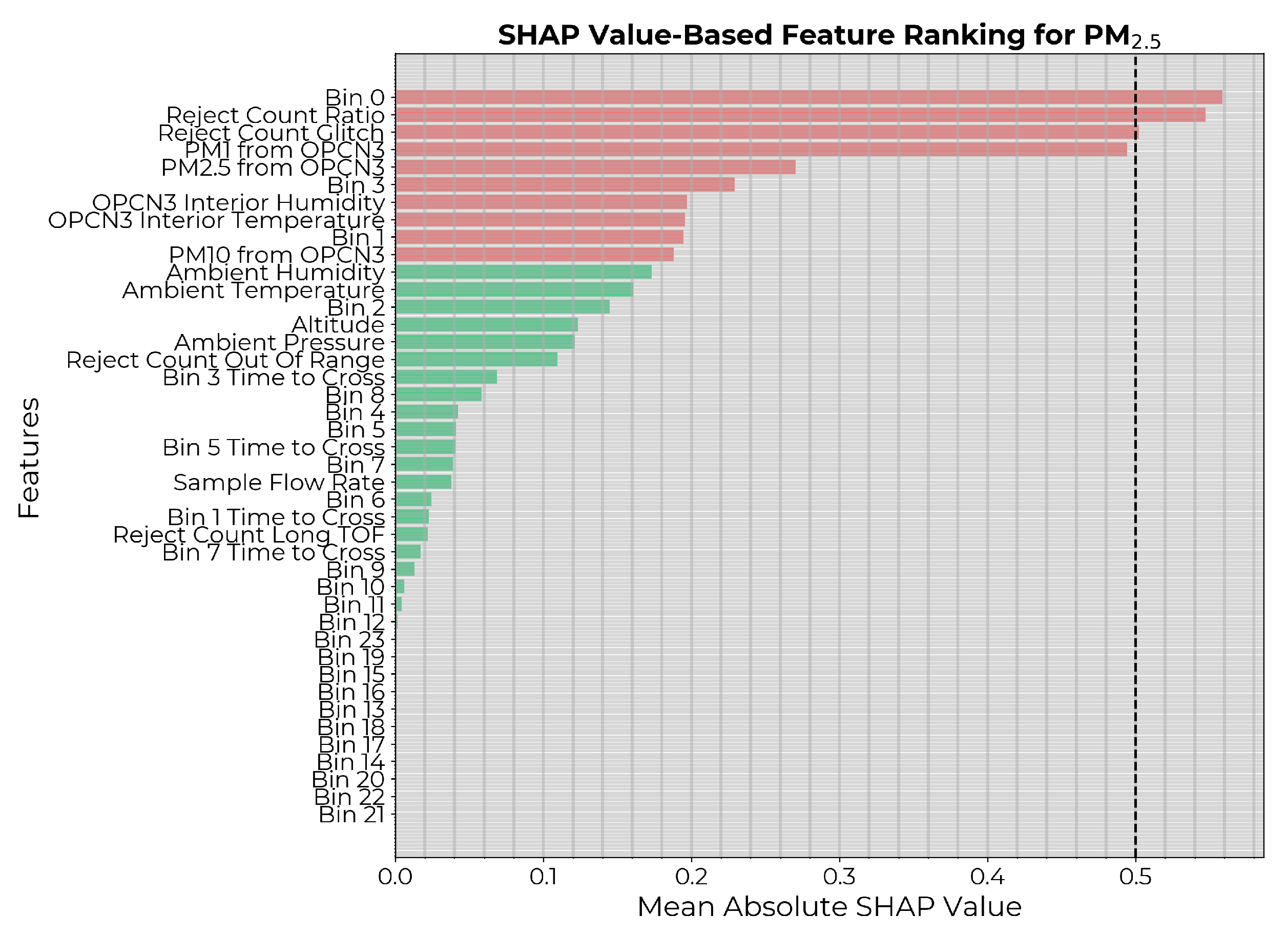
Figure 5.
Potential input features to the PM2.5 calibration model ranked in descending order of strength of causal influence after eliminating features with p-value. The 10 highest ranked features are highlighted in red.
Figure 5.
Potential input features to the PM2.5 calibration model ranked in descending order of strength of causal influence after eliminating features with p-value. The 10 highest ranked features are highlighted in red.
3. Results
In this section, we present the results from each of the three approaches across the two test cases.
PM1
The Table 1 depicts the performance evaluation metrics of the calibration model for PM1 derived from each approach, when applied on the independent test dataset. The causality-based feature selection is observed to yield the lowest MSE as well as the highest on the test dataset, demonstrating superior generalizability to unseen data and enhanced predictive performance. Therefore, the causality-based approach is clearly more adept at extracting the causal variables while eliminating the redundant, non-causal and/or indirect influences on the target. It also uses the least number of input features to the model out of the three. This improves computational efficiency, which is particularly valuable when sensors are deployed in the long term and at finer spatial resolutions in order to reduce the computational load of handling large datasets over extended periods.
Figure 6 shows the density plots of the residuals (that is, differences between the actual and predicted values) for each approach. Figure 7 depicts the scatter diagrams of the calibration model for PM1 under different feature selection approaches. Figure 7a–c show the scatter plots of true vs estimated PM1 count for each model on the train (blue) and independent test (red) sets. Figure 7d compares the performance of each model on the test set, with the causality-based approach yielding a comparatively thinner divergence from the 1:1 line. The density curve derived from the causality-based method exhibits a prominent density peak and narrower spread compared to the other two, indicating the most accurate predictions of the three, with fewer large residuals, thus producing a more reliable and robust model with fewer prediction errors.
PM2.5
The Table 2 presents the performance metrics of the PM2.5 calibration model derived from each approach evaluated on the independent test dataset.
Although MSEs are higher and the values are lower across all three approaches compared to PM1 calibration models, the causality-based feature selection method consistently yields the lowest MSE and the highest by a reasonable margin, with the least number of input features to the model.

Table 2.
The performance evaluation metrics for the estimation of PM2.5.
| Feature Selection Approach | Features used as Predictors | Number of Predictors | MSE | |
|---|---|---|---|---|
| No feature selection | All 42 outputs from the LCS | 42 | 0.41 | 0.977 |
| SHAP value-based | Bin 0, | 9 | 0.286 | 0.984 |
| Reject Count Ratio, | ||||
| Reject Count Glitch, | ||||
| Bin 3, | ||||
| PM1 from OPCN3, | ||||
| PM2.5 from OPCN3, | ||||
| OPCN3 Interior Temperature, | ||||
| OPCN3 Interior Humidity, | ||||
| Bin 1 | ||||
| Causality-based | Bin 0, | 7 | 0.274 | 0.985 |
| PM1 from OPCN3, | ||||
| PM2.5 from OPCN3, | ||||
| Reject Count Ratio, | ||||
| Ambient Temperature, | ||||
| Ambient Pressure, | ||||
| Ambient Humidity |
The Figure 8 depicts the density plots of the residuals for the PM2.5 estimation. Both models incorporating feature selection exhibit improved accuracy compared to the model without feature selection. Although less pronounced than in the case of PM1 models, the causality-based model continues to exhibit the narrowest residual distribution over larger values, characterized by a smaller base spread and a slightly higher peak compared to the SHAP value-based approach.
The Figure 9 gives the scatter diagrams of the calibration model for PM2.5 under different feature selection approaches, along with the comparison of the models’ performance on the test set. Again, though less pronounced than in the case of PM1 models, the causality-based approach yields the thinnest divergence from the 1:1 line.
4. Discussion
Our results demonstrate the efficacy of the causality-based feature selection method in building more accurate and robust calibration models for LCS that generalize better to unseen data.
We have compared the performance of the proposed method with feature selection based on SHAP values, a common approach for machine learning practitioners [47]. The proposed causality-based feature selection method consistently outperforms the SHAP value-based approach. It is important to note that in an effort to provide a rigorous and thorough comparison with the proposed method, we have opted for a minimal threshold ( in both test cases) for feature selection based on SHAP values. Therefore, the observed underperformance of the SHAP-based approach highlights its limitations in extracting causal information and reinforces the susceptibility of machine learning models to spurious correlations.
In both case studies, the features chosen as predictors from the proposed causal approach validate its ability to extract the most direct causal influences from mere correlations and indirect influences. In both instances, the reject count ratio has been extracted as an important predictor. This can be attributed to the operational principles of the OPC-N3. The OPC-N3 comprises of two photo diodes that record voltages which are subsequently translated into particle count data. Particles partially within the detection beam or passing near its edges are rejected and that is reflected on the parameter “Reject count ratio”. Consequently, this parameter enhances particle sizing accuracy, hence having a direct influence on the PM count [10]. Several studies have recorded the impact of meteorological parameters such as atmospheric pressure, temperature and humidity on atmospheric levels of PM [48,49,50,51,52,53,54]. Atmospheric pressure affects PM levels through its impact on air density, vertical mixing, and the transport and dispersion of particles. Atmospheric pressure obstructs the upward movement of particles. Under high-pressure systems, air tends to be more stable, trapping pollutants near the surface, increasing PM levels. In contrast, in lower-pressure conditions, particles may disperse more easily due to reduced air density. Temperature also affects atmospheric stability, changing how pollutants disperse. Hot weather often results in stagnant air conditions, which can trap PM and hinder its dispersion. In addition, elevated temperatures can speed up chemical reactions that generate PM, particularly in areas with vehicle and industrial emissions. Humidity influences ambient levels of PM significantly through hygroscopic growth: certain atmospheric species absorb water and increase in size once the relative humidity exceeds the deliquescence point of the substance. This phenomenon can shift smaller particles into larger PM size categories, resulting in changed PM levels. High humidity can also promote chemical reactions, such as the conversion of sulfur dioxide to sulfate aerosols [55], leading to higher PM levels. In addition to the direct impact of meteorological factors on ambient PM levels, the performance of LCS can also be influenced by these environmental conditions [56]. Therefore, naturally, ambient temperature, pressure, and humidity should be important predictors to the calibration model, which causality-based feature selection has been able to extract, as opposed to the SHAP value-based approach, which has placed greater import on temperature and humidity in the interior of the OPC leading to less accurate predictions on the test data.
Although this study focuses on the proposed feature selection method in the context of LCS calibration, it is broadly applicable to other machine learning tasks that involve time series data. The flexibility of CCM, which can handle both linear and nonlinear dynamics, as well as deterministic and random data without specific assumptions, enhances the utility of the proposed feature selection approach. However, a key limitation is that CCM requires a sufficiently long time series to reliably determine causality, which may pose challenges in cases where data is not collected in continuous intervals.
5. Conclusions
In this study, we propose a causality-based feature selection method using convergent cross mapping for the calibration of low-cost air quality sensor systems using machine learning. Integration of causality improves the interpretability and generalizability of environmental machine learning models. Application of this approach to real-world low-cost sensor calibration demonstrates significant improvements in predictive performance and generalizability, confirming the efficacy of the proposed methodology.
In future work, we aim to validate this approach across various types of sensors and datasets to assess its robustness and adaptability in a range of applications in atmospheric and climate sciences. In particular, the mathematical rigor and versatility of convergent cross mapping, which underpins our feature selection method, could prove advantageous in empirical climate modeling applications.
Author Contributions
“Conceptualization, V.S. and D.J.L.; methodology, V.S. and D.J.L.;data curation, L.O.H.W.; software, V.S.; validation, D.J.L.; formal analysis, V.S.; investigation, V.S.; resources, D.J.L. and L.O.H.W.; ;writing—original draft preparation, V.S.; writing—review and editing, D.J.L., V.S. and L.O.H.W.; visualization, V.S.; supervision, D.J.L.; project administration, D.J.L.; funding acquisition, D.J.L. All authors have read and agreed to the published version of the manuscript.
Funding
This research was funded by TRECIS CC* Cyberteam (NSF #2019135); NSF OAC-2115094 Award; and EPA P3 grant number 84057001-0.; AFWERX AFX23D-TCSO1 Proposal # F2-17492.
Institutional Review Board Statement
Not applicable.
Informed Consent Statement
Not applicable
Data Availability Statement
The code and data are publicly available at https://github.com/mi3nts/Causality-Driven-Machine-Learning.
Acknowledgments
Not applicable.
Conflicts of Interest
The authors declare no conflicts of interest.
Abbreviations
The following abbreviations are used in this manuscript:
| PM | Particulate matter |
| IoT | Internet of Things |
| LCS | Low-cost air quality sensor systems |
| ML | Machine learning |
| CCM | Convergent cross mapping |
| OPC | Optical particle counter |
| MSE | Mean Squared Error |
References
- Intergovernmental Panel on Climate Change. Climate Change 2021: The Physical Science Basis. Contribution of Working Group I to the Sixth Assessment Report of the Intergovernmental Panel on Climate Change; Cambridge University Press: Cambridge, United Kingdom and New York, NY, USA, 2021. In press, . [CrossRef]
- Orru, H.; Ebi, K.; Forsberg, B. The interplay of climate change and air pollution on health. Current environmental health reports 2017, 4, 504–513. [CrossRef]
- Arshad, K.; Hussain, N.; Ashraf, M.H.; Saleem, M.Z.; others. Air pollution and climate change as grand challenges to sustainability. Science of The Total Environment 2024, p. 172370. [CrossRef]
- Shaddick, G.; Thomas, M.L.; Mudu, P.; Ruggeri, G.; Gumy, S. Half the world’s population are exposed to increasing air pollution. NPJ Climate and Atmospheric Science 2020, 3, 1–5. [CrossRef]
- Li, Y.; Xu, L.; Shan, Z.; Teng, W.; Han, C. Association between air pollution and type 2 diabetes: an updated review of the literature. Therapeutic advances in endocrinology and metabolism 2019, 10, 2042018819897046. [CrossRef]
- Nolte, C.; others. Air quality. In Impacts, risks, and adaptation in the United States: Fourth national climate assessment, volume II; U.S. Global Change Research Program: Washington, DC, 2018; chapter 13, p. 516.
- Organization, W.M.; Programme, U.N.E.; project, I.G.A.C. Low-cost air quality sensor systems (LCS) for policy-relevant air quality analysis. Gaw report no. 293, World Meteorological Organization, Geneva, 2024. Lead coordinating author: Carl Malings. Contributing authors: Jan-Michael Archer, África Barreto, Jianzhao Bi, and others.
- Okafor, N.U.; Alghorani, Y.; Delaney, D.T. Improving data quality of low-cost IoT sensors in environmental monitoring networks using data fusion and machine learning approach. ICT Express 2020, 6, 220–228. [CrossRef]
- DeSouza, P.; Kahn, R.; Stockman, T.; Obermann, W.; Crawford, B.; Wang, A.; Crooks, J.; Li, J.; Kinney, P. Calibrating networks of low-cost air quality sensors. Atmospheric Measurement Techniques 2022, 15, 6309–6328. [CrossRef]
- Wijeratne, L.O.; Kiv, D.R.; Aker, A.R.; Talebi, S.; Lary, D.J. Using machine learning for the calibration of airborne particulate sensors. Sensors 2019, 20, 99. [CrossRef]
- Zhang, Y.; Wijeratne, L.O.; Talebi, S.; Lary, D.J. Machine learning for light sensor calibration. Sensors 2021, 21, 6259. [CrossRef]
- Wang, A.; Machida, Y.; deSouza, P.; Mora, S.; Duhl, T.; Hudda, N.; Durant, J.L.; Duarte, F.; Ratti, C. Leveraging machine learning algorithms to advance low-cost air sensor calibration in stationary and mobile settings. Atmospheric Environment 2023, 301, 119692. [CrossRef]
- Kelly, B.; Xiu, D.; others. Financial machine learning. Foundations and Trends® in Finance 2023, 13, 205–363. [CrossRef]
- Mariani, M.M.; Borghi, M. Artificial intelligence in service industries: customers’ assessment of service production and resilient service operations. International Journal of Production Research 2024, 62, 5400–5416. [CrossRef]
- Rajkomar, A.; Dean, J.; Kohane, I. Machine learning in medicine. New England Journal of Medicine 2019, 380, 1347–1358. [CrossRef]
- Kang, Z.; Catal, C.; Tekinerdogan, B. Machine learning applications in production lines: A systematic literature review. Computers & Industrial Engineering 2020, 149, 106773. [CrossRef]
- Lary, D.J.; Zewdie, G.K.; Liu, X.; Wu, D.; Levetin, E.; Allee, R.J.; Malakar, N.; Walker, A.; Mussa, H.; Mannino, A.; others. Machine learning applications for earth observation. Earth observation open science and innovation 2018, 165. [CrossRef]
- Malakar, N.K.; Lary, D.J.; Moore, A.; Gencaga, D.; Roscoe, B.; Albayrak, A.; Wei, J. Estimation and bias correction of aerosol abundance using data-driven machine learning and remote sensing. 2012 Conference on Intelligent Data Understanding. IEEE, 2012, pp. 24–30.
- Albayrak, A.; Wei, J.; Petrenko, M.; Lary, D.; Leptoukh, G. Modis aerosol optical depth bias adjustment using machine learning algorithms. AGU Fall Meeting Abstracts, 2011, Vol. 2011, pp. A53C–0371.
- Rudner, T.G.J.; Toner, H. Key Concepts in AI Safety: Interpretability in Machine Learning. 2021.
- Doshi-Velez, F.; Kim, B. Towards A Rigorous Science of Interpretable Machine Learning. arXiv: Machine Learning 2017.
- Lipton, Z.C. The mythos of model interpretability: In machine learning, the concept of interpretability is both important and slippery. Queue 2018, 16, 31–57. [CrossRef]
- Lundberg, S. A unified approach to interpreting model predictions. arXiv preprint arXiv:1705.07874 2017.
- Li, K.; DeCost, B.; Choudhary, K.; Greenwood, M.; Hattrick-Simpers, J. A critical examination of robustness and generalizability of machine learning prediction of materials properties. npj Computational Materials 2023, 9, 55. [CrossRef]
- Schölkopf, B. Causality for machine learning. In Probabilistic and causal inference: The works of Judea Pearl; 2022; pp. 765–804.
- Cloudera Fast Forward Labs. Causality for Machine Learning: Applied Research Report. https://ff13.fastforwardlabs.com/, 2020.
- Beery, S.; Van Horn, G.; Perona, P. Recognition in terra incognita. Proceedings of the European conference on computer vision (ECCV), 2018, pp. 456–473.
- Ye, W.; Zheng, G.; Cao, X.; Ma, Y.; Hu, X.; Zhang, A. Spurious correlations in machine learning: A survey. arXiv preprint arXiv:2402.12715 2024.
- Ilyas, A.; Santurkar, S.; Tsipras, D.; Engstrom, L.; Tran, B.; Madry, A. Adversarial examples are not bugs, they are features. Advances in neural information processing systems 2019, 32.
- Haavelmo, T. The probability approach in econometrics. Econometrica 1944, 12, S1–S115 (supplement). [CrossRef]
- Bühlmann, P. Invariance, causality and robustness. Statistical Science 2020, 35, 404–426.
- Peters, J.; Bühlmann, P.; Meinshausen, N. Causal inference by using invariant prediction: identification and confidence intervals. Journal of the Royal Statistical Society Series B: Statistical Methodology 2016, 78, 947–1012. [CrossRef]
- Ribeiro, M.T.; Singh, S.; Guestrin, C. " Why should i trust you?" Explaining the predictions of any classifier. Proceedings of the 22nd ACM SIGKDD international conference on knowledge discovery and data mining, 2016, pp. 1135–1144.
- Sugihara, G.; May, R.; Ye, H.; Hsieh, C.h.; Deyle, E.; Fogarty, M.; Munch, S. Detecting causality in complex ecosystems. science 2012, 338, 496–500. [CrossRef]
- Tsonis, A.A.; Deyle, E.R.; May, R.M.; Sugihara, G.; Swanson, K.; Verbeten, J.D.; Wang, G. Dynamical evidence for causality between galactic cosmic rays and interannual variation in global temperature. Proceedings of the National Academy of Sciences 2015, 112, 3253–3256. [CrossRef]
- Takens, F. Detecting strange attractors in turbulence. Dynamical Systems and Turbulence, Warwick 1980: proceedings of a symposium held at the University of Warwick 1979/80. Springer, 2006, pp. 366–381.
- Sun, Y.N.; Qin, W.; Hu, J.H.; Xu, H.W.; Sun, P.Z. A causal model-inspired automatic feature-selection method for developing data-driven soft sensors in complex industrial processes. Engineering 2023, 22, 82–93. [CrossRef]
- Chen, Z.; Cai, J.; Gao, B.; Xu, B.; Dai, S.; He, B.; Xie, X. Detecting the causality influence of individual meteorological factors on local PM2. 5 concentration in the Jing-Jin-Ji region. Scientific Reports 2017, 7, 40735. [CrossRef]
- Rybarczyk, Y.; Zalakeviciute, R.; Ortiz-Prado, E. Causal effect of air pollution and meteorology on the COVID-19 pandemic: A convergent cross mapping approach. Heliyon 2024, 10. [CrossRef]
- Ye, H.; Deyle, E.R.; Gilarranz, L.J.; Sugihara, G. Distinguishing time-delayed causal interactions using convergent cross mapping. Scientific reports 2015, 5, 14750. [CrossRef]
- Javier, P.J.E. causal-ccm: A Python implementation of Convergent Cross Mapping (Version 0.3.3). https://github.com/javier/causal-ccm, 2021. Computer software.
- Edwards, A.W. RA Fischer, statistical methods for research workers, (1925). In Landmark writings in western mathematics 1640-1940; Elsevier, 2005; pp. 856–870.
- Wasserstein, R.L.; Lazar, N.A. The ASA statement on p-values: context, process, and purpose, 2016.
- Alphasense. Alphasense User Manual OPC-N3 Optical Particle Counter. Great Notley, UK, 2018.
- Broich, A.V.; Gerharz, L.E.; Klemm, O. Personal monitoring of exposure to particulate matter with a high temporal resolution. Environmental Science and Pollution Research 2012, 19, 2959–2972. [CrossRef]
- Sugihara, G.; May, R.M. Nonlinear forecasting as a way of distinguishing chaos from measurement error in time series. Nature 1990, 344, 734–741. [CrossRef]
- Marcílio, W.E.; Eler, D.M. From explanations to feature selection: assessing SHAP values as feature selection mechanism. 2020 33rd SIBGRAPI conference on Graphics, Patterns and Images (SIBGRAPI). Ieee, 2020, pp. 340–347.
- Kirešová, S.; Guzan, M. Determining the correlation between particulate matter PM10 and meteorological factors. Eng 2022, 3, 343–363. [CrossRef]
- Yang, H.; Peng, Q.; Zhou, J.; Song, G.; Gong, X. The unidirectional causality influence of factors on PM2. 5 in Shenyang city of China. Sci Rep 10: 8403, 2020. [CrossRef]
- Fu, H.; Zhang, Y.; Liao, C.; Mao, L.; Wang, Z.; Hong, N. Investigating PM2. 5 responses to other air pollutants and meteorological factors across multiple temporal scales. Scientific reports 2020, 10, 15639. [CrossRef]
- Vaishali.; Verma, G.; Das, R.M. Influence of temperature and relative humidity on PM2. 5 concentration over Delhi. MAPAN 2023, 38, 759–769. [CrossRef]
- Hernandez, G.; Berry, T.A.; Wallis, S.L.; Poyner, D. Temperature and humidity effects on particulate matter concentrations in a sub-tropical climate during winter. International proceedings of chemical, biological and environmental engineering 2017, 102, 41–49.
- Kim, M.; Jeong, S.G.; Park, J.; Kim, S.; Lee, J.H. Investigating the impact of relative humidity and air tightness on PM sedimentation and concentration reduction. Building and Environment 2023, 241, 110270. [CrossRef]
- Zhang, M.; Chen, S.; Zhang, X.; Guo, S.; Wang, Y.; Zhao, F.; Chen, J.; Qi, P.; Lu, F.; Chen, M.; others. Characters of particulate matter and their relationship with meteorological factors during winter Nanyang 2021–2022. Atmosphere 2023, 14, 137. [CrossRef]
- Zhang, S.; Xing, J.; Sarwar, G.; Ge, Y.; He, H.; Duan, F.; Zhao, Y.; He, K.; Zhu, L.; Chu, B. Parameterization of heterogeneous reaction of SO2 to sulfate on dust with coexistence of NH3 and NO2 under different humidity conditions. Atmospheric Environment 2019, 208, 133–140. [CrossRef]
- Raysoni, A.U.; Pinakana, S.D.; Mendez, E.; Wladyka, D.; Sepielak, K.; Temby, O. A Review of Literature on the Usage of Low-Cost Sensors to Measure Particulate Matter. Earth 2023, 4, 168–186. [CrossRef]
| 1 | While p-values are used to quantify the statistical significance of a result, a higher p-value alone may be insufficient grounds to dismiss a result [43]. Therefore, we recommend due caution when implementing the elimination outlined in Step 2. For the test cases presented in the current study, all with p-value were observed to have negligibly small values and therefore unlikely to impart useful information to the model. As an additional verification, the performance of the model after elimination was compared to that of the full model, and it was observed that the performance improved, thus validating the removal of the features. |
Figure 2.
Input features to the PM1 calibration model ranked in descending order of mean absolute SHAP value. The 10 highest-ranked features are highlighted in red.
Figure 2.
Input features to the PM1 calibration model ranked in descending order of mean absolute SHAP value. The 10 highest-ranked features are highlighted in red.
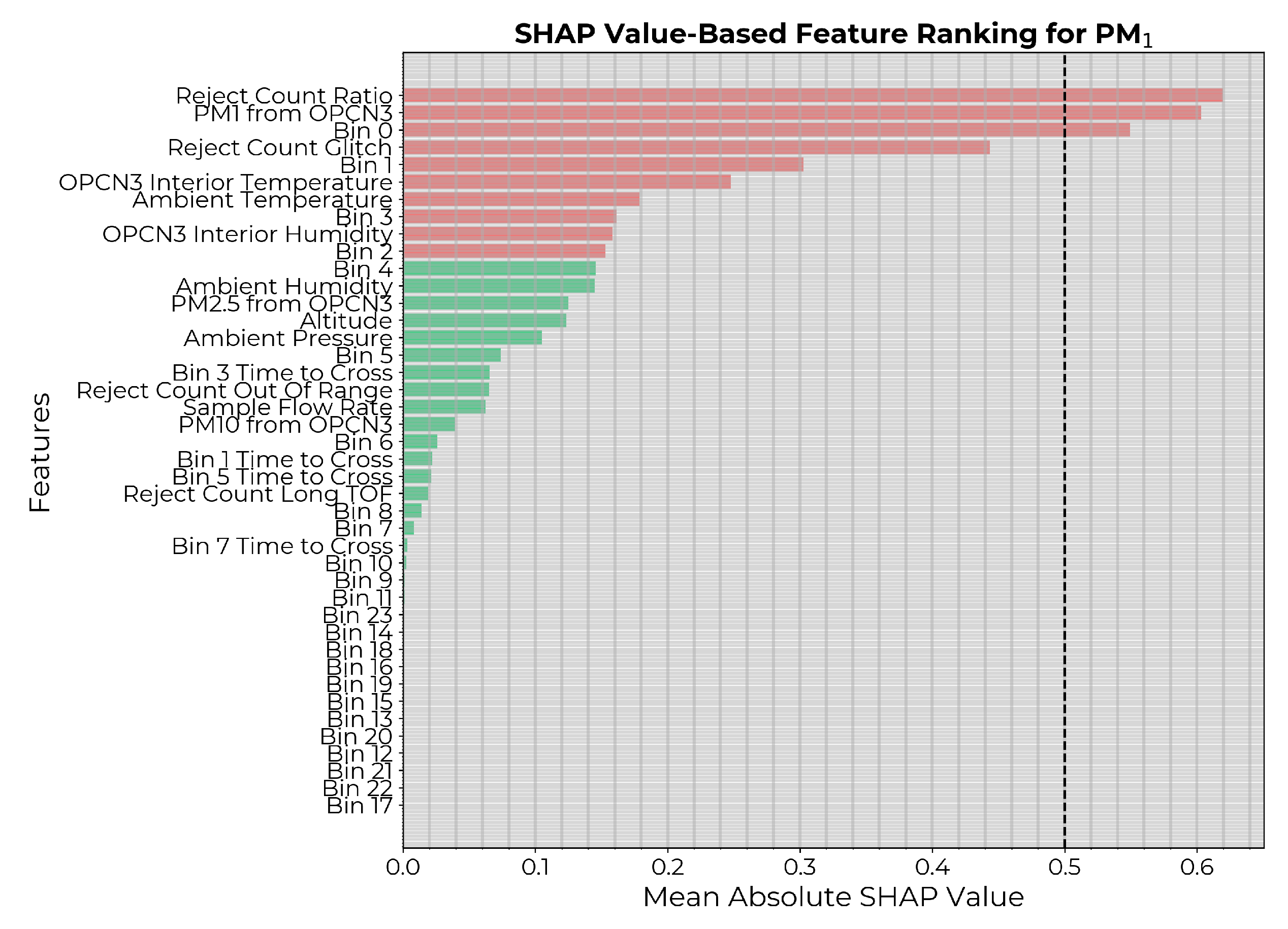
Figure 3.
Potential input features to the PM1 calibration model ranked in descending order of strength of causal influence after eliminating features with p-value. The 10 highest ranked features are highlighted in red.
Figure 3.
Potential input features to the PM1 calibration model ranked in descending order of strength of causal influence after eliminating features with p-value. The 10 highest ranked features are highlighted in red.
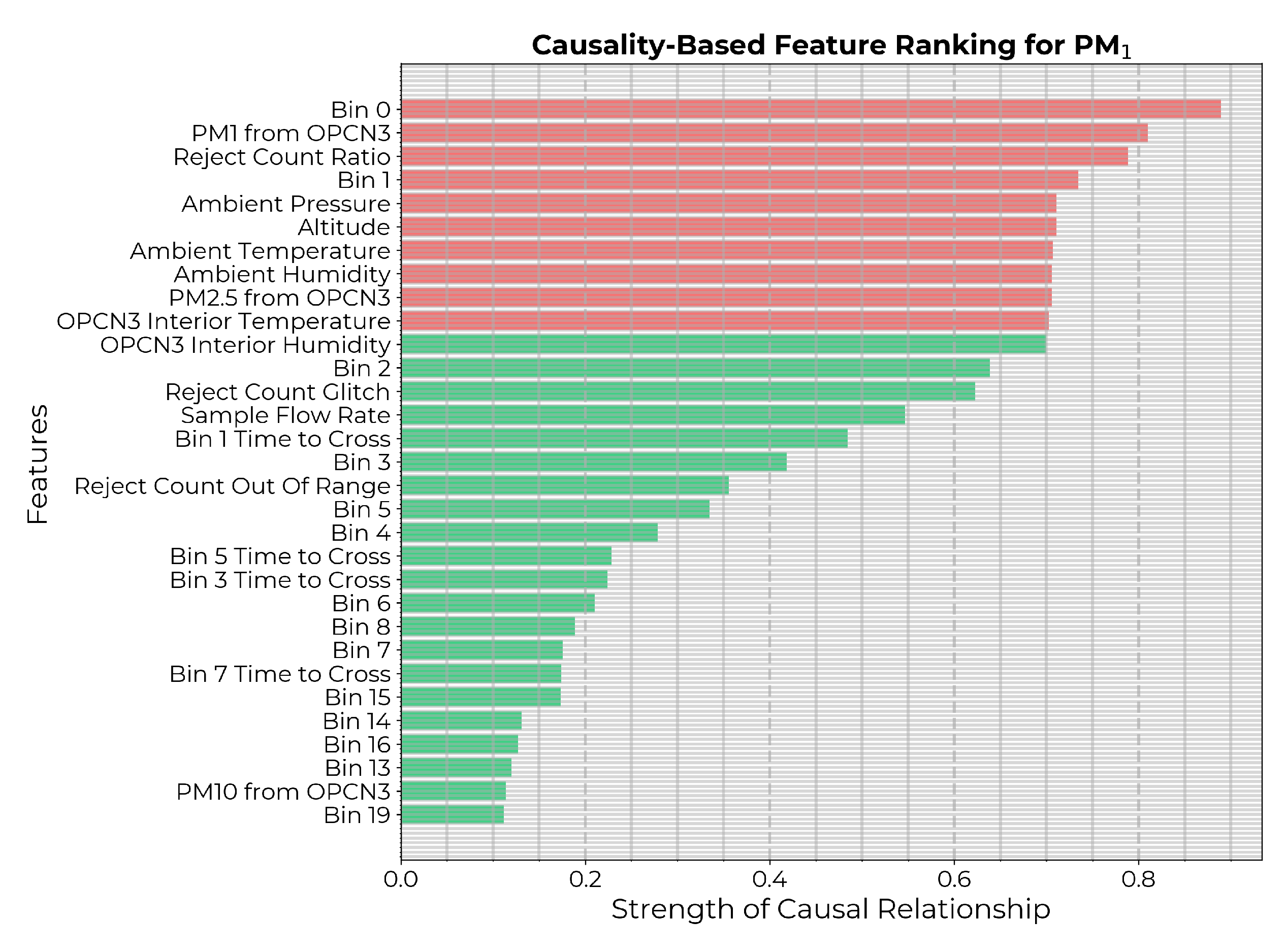
Figure 6.
Density plots of the residuals for the PM1 calibration models derived from each approach.
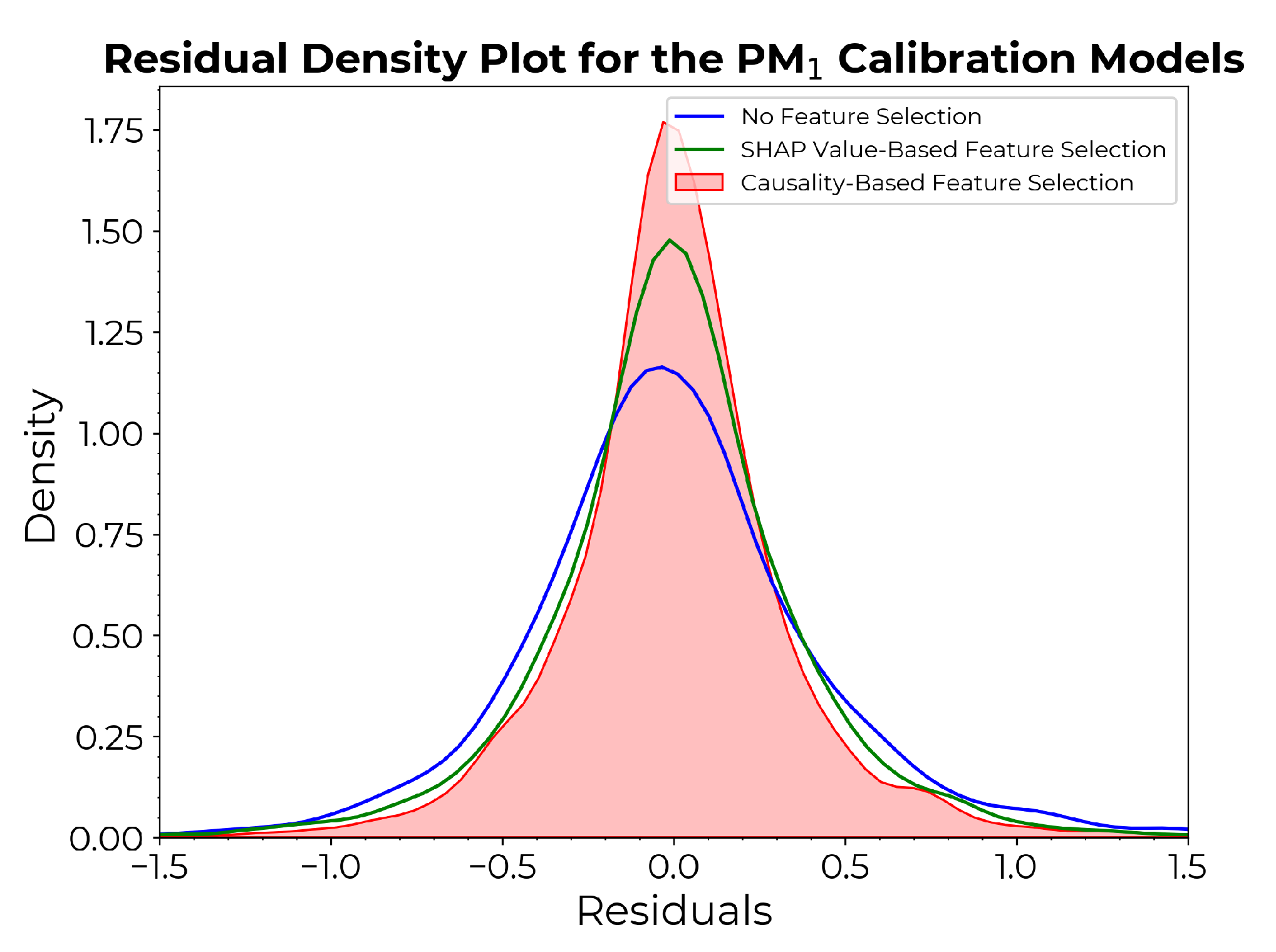
Figure 7.
Scatter diagrams for the calibration models with the x-axis showing the PM1 count from the reference instrument and the y-axis showing the PM1 count provided by calibrating the LCS: (a) Without any feature selection. (b) SHAP value-based feature selection. (c) Causality-based feature selection. (d) Comparison of true vs predicted values for the test set across models .
Figure 7.
Scatter diagrams for the calibration models with the x-axis showing the PM1 count from the reference instrument and the y-axis showing the PM1 count provided by calibrating the LCS: (a) Without any feature selection. (b) SHAP value-based feature selection. (c) Causality-based feature selection. (d) Comparison of true vs predicted values for the test set across models .
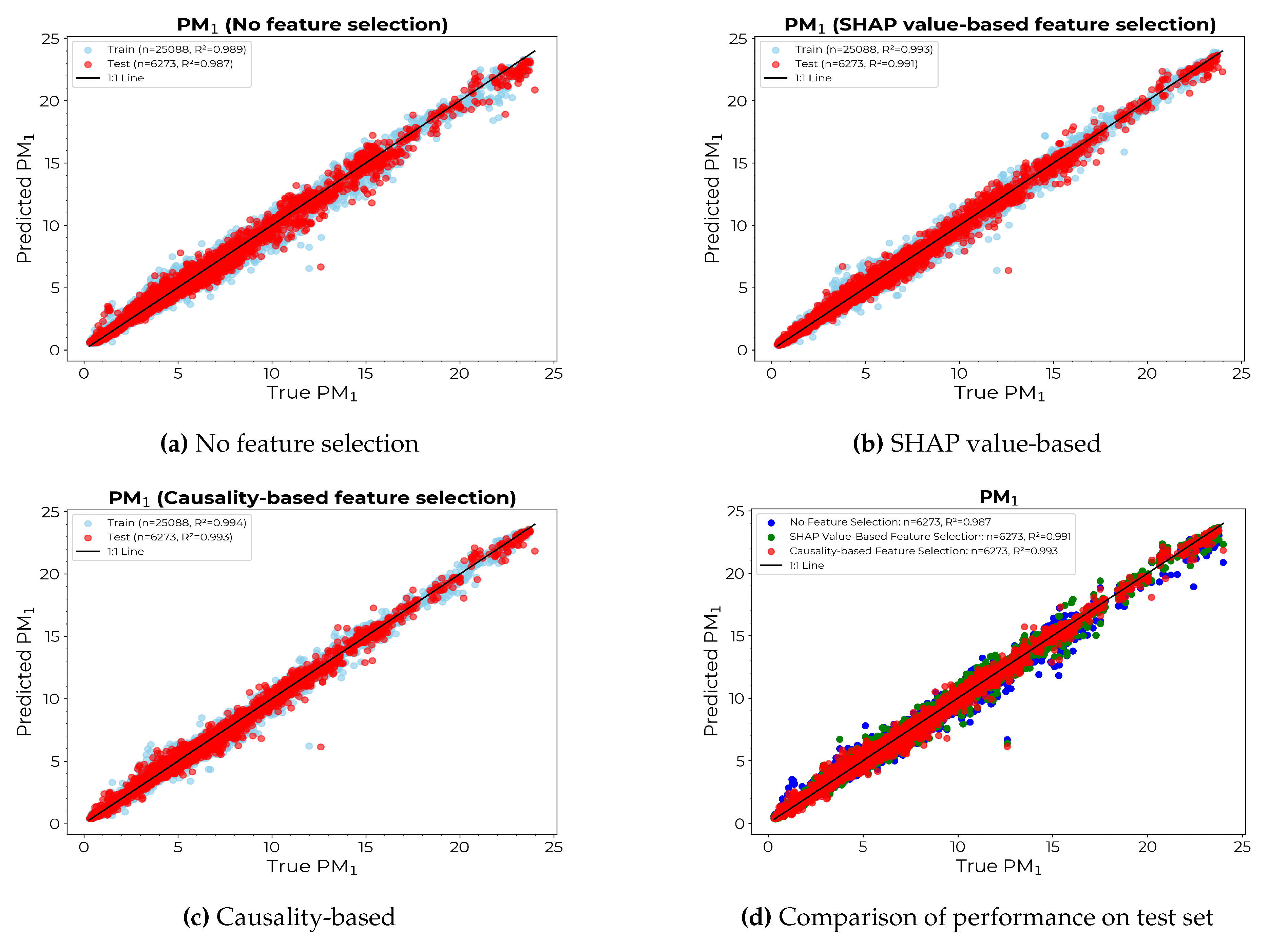
Figure 8.
Density plots of the residuals for the PM2.5 calibartion models derived from each approach.
Figure 8.
Density plots of the residuals for the PM2.5 calibartion models derived from each approach.
Figure 9.
Scatter diagrams for the calibration models with the x-axis showing the PM2.5 count from the reference instrument and the y-axis showing the PM2.5 count provided by calibrating the LCS: (a) Without any feature selection. (b) SHAP value-based feature selection. (c) Causality-based feature selection. (d) Comparison of true vs predicted values for the test set across models .
Figure 9.
Scatter diagrams for the calibration models with the x-axis showing the PM2.5 count from the reference instrument and the y-axis showing the PM2.5 count provided by calibrating the LCS: (a) Without any feature selection. (b) SHAP value-based feature selection. (c) Causality-based feature selection. (d) Comparison of true vs predicted values for the test set across models .
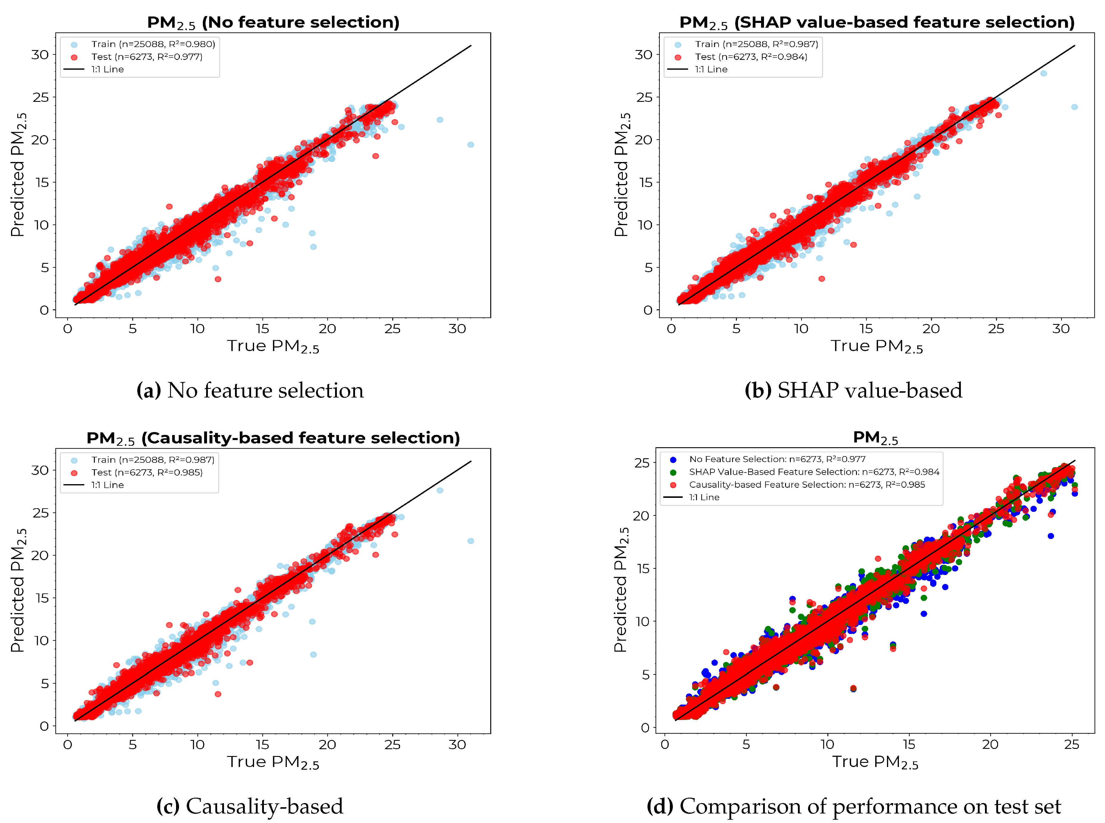
Table 1.
The performance evaluation metrics for the estimation of PM1.
| Feature Selection Approach | Features used as Predictors | Number of Predictors | MSE | |
|---|---|---|---|---|
| No feature selection | All 42 outputs from the LCS | 42 | 0.213 | 0.987 |
| SHAP value-based | Reject Count Ratio, | 6 | 0.150 | 0.991 |
| PM1 from OPCN3, | ||||
| Reject Count Glitch, | ||||
| OPCN3 Interior Temperature, | ||||
| Ambient Temperature, | ||||
| OPCN3 Interior Humidity | ||||
| Causality-based | Bin 0, | 5 | 0.121 | 0.993 |
| Reject Count Ratio, | ||||
| Ambient Pressure, | ||||
| Ambient Temperature, | ||||
| Ambient Humidity |
Disclaimer/Publisher’s Note: The statements, opinions and data contained in all publications are solely those of the individual author(s) and contributor(s) and not of MDPI and/or the editor(s). MDPI and/or the editor(s) disclaim responsibility for any injury to people or property resulting from any ideas, methods, instructions or products referred to in the content. |
© 2024 by the authors. Licensee MDPI, Basel, Switzerland. This article is an open access article distributed under the terms and conditions of the Creative Commons Attribution (CC BY) license (http://creativecommons.org/licenses/by/4.0/).
Copyright: This open access article is published under a Creative Commons CC BY 4.0 license, which permit the free download, distribution, and reuse, provided that the author and preprint are cited in any reuse.


