
Submitted:
07 October 2024
Posted:
09 October 2024
You are already at the latest version
Abstract
The human brain, a highly complex dynamical system, exhibits various states of consciousness—such as wakefulness, sleep, and altered states—each characterized by distinct patterns of neural activity. To capture the dynamical properties of these states, a range of complexity measures is utilized, with a primary focus on Statistical Complexity (SC) and Lempel-Ziv complexity (LZc), and supplemented by Approximate Entropy (ApEn) and Kolmogorov Complexity (KC). These measures are applied to both simulated data, generated through logistic maps and Multivariate Autoregressive (MVAR) models, and intracranial depth electrode recordings from patients. The results demonstrate that these complexity measures effectively capture intricate dynamics of the brain across different states. Specifically, SC captures the structural complexity and information processing within the system, reflecting organized and predictive neural behavior by accounting for temporal correlations in the data. In contrast, LZc is more sensitive to randomness, measuring the diversity and unpredictability of patterns within the data. This distinction allows SC to serve as a more reliable indicator of organized information processing, while LZc highlights the variability in neural signals. Notably, the study reveals that states of higher consciousness are associated with greater complexity, supporting the entropic brain hypothesis. This research contributes to the ongoing efforts to quantify consciousness through mathematical frameworks and offers insights into the neural correlates of different states of awareness.
Keywords:
complexity measures
; states of consciousness
; time series
; dynamical systems
Codes: Find appropriate codes at https://github.com/Odanson/Complexity-Measures-Consciousness-Analysis
1. Introduction
Understanding the nature of consciousness has long been a significant challenge in both the scientific and philosophical realms. In recent years, the study of complexity has provided a new perspective on this age-old problem. Complexity science, which examines how interactions within a system give rise to collective behaviors, offers valuable tools for analyzing the dynamical regimes associated with different states of consciousness.
The human brain is a highly complex dynamical system, and various states of
consciousness—such as wakefulness, sleep, and altered states induced by meditation or substances—can be viewed through the lens of complexity. Chaotic dynamical systems, characterized by sensitivity to initial conditions and long-term unpredictability, serve as a fundamental model for understanding the brain’s complex behavior [1,2]. By employing measures from complexity science, these states can be quantified and analyzed in a rigorous manner. This dissertation aims to explore and apply several complexity measures to different dynamical regimes, with a particular focus on states of consciousness.
Complexity measures such as Lempel-Ziv complexity (LZc), Statistical Complexity (SC), Approximate Entropy (ApEn), and Kolmogorov Complexity (KC) have been shown to differentiate between various states of consciousness. Lempel-Ziv complexity quantifies the compressibility of a sequence by identifying the number of distinct patterns or substrings within it[3], with higher values indicating greater diversity and randomness in the sequence. Statistical complexity captures the structural complexity of a time series by evaluating the amount of information stored in the system [4]. Approximate entropy assesses the regularity and unpredictability of fluctuations in a time series, focusing on the likelihood that similar patterns of observations will not be followed by additional similar observations [5]. Kolmogorov complexity evaluates the complexity of a sequence based on the length of the shortest possible description (or program) that can produce the sequence, reflecting the inherent randomness and informational content of the sequence [6].
Recent studies have demonstrated that global states of consciousness can be effectively differentiated using measures of temporal differentiation, which assess the number or entropy of temporal patterns in neurophysiological time series [7]. Temporal differentiation refers to how varied a time series is over time. Typically, time series from unconscious states, such as general anesthesia and NREM sleep, display less temporal differentiation compared to those from awake states [8,9,10,11,12,13]. These observations align with the entropic brain hypothesis, which posits that higher temporal differentiation correlates with richer and more diverse conscious experiences [14,15,16,17].
In parallel with these advances, Integrated Information Theory (IIT) has emerged as a leading theoretical framework for understanding consciousness. IIT posits that consciousness corresponds to the capacity of a system to integrate information, quantified by a measure known as [18]. represents the degree to which a system’s informational content is greater than the sum of its parts, reflecting the system’s ability to produce a unified, integrated experience [19,20]. Despite its conceptual elegance, the practical application of is severely limited by the immense computational complexity required to calculate it in real-world systems like the human brain [21,22].
Given the challenges of directly measuring , researchers have explored alternative methods to approximate the integrated information in the brain. The Perturbational Complexity Index (PCI) has been introduced as an empirical proxy for [10]. PCI is derived from the brain’s response to transcranial magnetic stimulation (TMS) and measures the complexity of the resulting EEG signals. By capturing both the integration and differentiation of neural activity, PCI aligns with the core principles of IIT and serves as a feasible measure of consciousness that can be applied across different states and clinical conditions.
Building on these foundations, this research seeks to investigate how these complexity measures vary across different dynamical regimes and how effectively they detect changes in both simulated and real-world data. It also explores their ability to distinguish between various sleep stages, revealing different aspects of brain dynamics. To achieve this, we utilize a range of models that represent different types of dynamical behavior: purely random data, the logistic map, and the multivariate autoregressive (MVAR) model.
Purely random data serves as a baseline model, representing a system with maximal entropy and minimal structure. This allows us to explore how complexity measures behave in the absence of deterministic patterns [23,24]. The logistic map is a simple yet powerful mathematical model that exhibits a wide range of behaviors, from periodic to chaotic, depending on the parameter settings [25,26]. It serves as a classic example of a chaotic system, making it an ideal candidate for testing how complexity measures respond to varying degrees of order and chaos. The multivariate autoregressive (MVAR) model is a more complex, data-driven approach that captures the relationships between multiple time series variables [27,28]. It is often used to model and analyze real-world systems like brain dynamics, offering a more realistic representation of how different brain regions interact over time.
The comparison of results from these models with those derived from real-world data is intended to assess the consistency and variability of these measures in practical applications. This approach contributes to a deeper understanding of consciousness through the interplay of complexity, information integration, and entropy.
1.1. Research Objectives
The primary aim of this research is to investigate the behaviours of complexity measures in different dynamical regimes and how these measures can be used to understand and differentiate between various states of consciousness. Specific objectives include:
- Applying statistical, informational, and dynamical complexity measures to simulated and real-world data.
- Examining the behavior of these measures in different dynamical regimes, such as chaotic and periodic systems.
- Comparing the effectiveness of complexity measures in capturing the dynamical properties of the systems studied.
2. Complexity Measures
2.1. Introduction to Complexity Measures
The concept of ’complexity’ is multifaceted, encompassing various definitions and applications across different fields. Complexity measures serve as indicators of certain characteristics inherent in a signal, allowing for the analysis, classification, and diagnostic assessment of signals. These measures are instrumental in distinguishing between different types of signals, such as periodic, quasiperiodic, chaotic, and random signals. Widely recognized complexity measures like Lempel-Ziv complexity (LZc) and approximate entropy (ApEn) are extensively used to characterize biological signals, providing insights into their underlying structures and dynamics [5,29,30].
Recently, Munoz et al. [4] applied a measure of statistical complexity (SC) that theoretically captures dynamical diversity. They studied local field potential data from fruit flies and found that SC decreased in general anesthesia compared with an ordinary waking state. This measure calculates the entropy of a time series, but with states specially defined such that if two sequences of observations lead to very similar probability distributions for future observations, those two sequences are considered identical microstates [31,32]. This approach contrasts with other complexity measures like LZc, which tends to take its maximum value for data that are maximally random [3].
The utility of complexity measures extend to various applications, including differentiating states of consciousness. For instance, Starkey et al. [32] demonstrated that SC can distinguish between different stages of sleep and between normal waking states and states induced by psychedelic substances like ketamine, lysergic acid diethylamide (LSD), and psilocybin. Their findings indicated that SC decreases during anesthesia and non-rapid eye movement (NREM) sleep but increases relative to placebo for all three psychedelic substances. This suggests that SC is a robust measure for investigating the complexity of neural activity associated with different states of consciousness.
2.2. Statistical Complexity
Statistical Complexity (SC) is a concept from computational mechanics that quantifies the minimal amount of information required to predict the future behavior of a stochastic process based on its past. It provides valuable insights into the underlying structure and predictability of complex systems [4,32]. SC is given by the Shannon entropy of an -machine fitted to a time series. An -machine is a prediction model that most efficiently predicts the future of a time series, assuming that the dependence between past and future states does not change over time [31]. The possible histories of the system are coarse-grained such that two histories are considered identical if the probability distribution for the future is the same for both histories. The statistical complexity is then the standard Shannon entropy over this coarse-graining.
In practice, when working with finite data, it is not possible to fit an -machine precisely, and several hyperparameter decisions must be made. Firstly, the length of history to be considered, referred to as the memory length (), must be selected. For an -machine to effectively predict a stochastic process with a Markov order of m, the memory length () must be at least m. Secondly, one must decide on the "probability distribution for the future," which involves choosing whether to consider only the next observation or a sequence of future observations. Lastly, a tolerance parameter () is required. This parameter ensures that two states are regarded as equivalent if their probability distributions of future states are sufficiently similar, meaning there is no future state for which the two states differ in the probability of leading to that state by more than [32].
In SC, high scores indicate significant signal diversity, with the dynamical evolution from distinct sequences needing to remain largely distinct. A distinctive feature of SC is that it generally follows an inverted U-shaped function in relation to randomness, peaking at intermediate levels of randomness. This contrasts with Lempel-Ziv complexity (LZc), which increases monotonically and reaches its highest values at maximum randomness [32,33]. For example, let’s consider a binary string and the computation of SC with the memory length parameter () set to 2. If the digit 0 is followed by 1 60% of the time and the digit 1 is followed by 0 80% of the time, the states 0 and 1 would be recognized as distinct, leading to a SC value greater than zero. Conversely, if the digit 0 is followed by 1 half the time, and the digit 1 is also followed by 1 half the time, then the states 0 and 1 would be considered identical in the -machine framework, resulting in a SC of zero. This is further illustrated in (Figure 1).
The relationship between SC and randomness can be further elucidated by contrasting it with syntactic information. Monotonic (deterministic) complexity, such as LZc, increases with randomness, capturing "syntactic information." In contrast, SC follows a convex function of randomness, capturing "pragmatic information" [33]. This difference highlights the unique capacity of SC to reflect meaningful structures within data rather than mere randomness (Figure 2).
2.3. Lempel-Ziv Complexity
Lempel-Ziv complexity (LZc) is a measure of the complexity of a finite sequence of data. It quantifies the number of distinct patterns or substrings within a given sequence, reflecting the diversity and regularity of the sequence. LZc has since evolved into a fundamental concept, eventually forming the foundation of the widely used zip compression algorithm [3,29,34]. This algorithm has also found significant applications in scientific research, particularly in the analysis of diverse patterns across various types of signals. For example, LZc has been extensively applied in neuroscience, especially in the study of EEG brain activity. Early research utilized LZc to explore conditions such as epilepsy [35] and the depth of anesthesia [8], while more recent studies have extended its application to various altered states of consciousness [13,32]. Beyond neuroscience, LZc has proven valuable in other fields as well, including the analysis of DNA sequence complexity [36] and ventricular fibrillation [37]. Its widespread use in biomedical data analysis underscores its status as a well-established and versatile tool in this domain [38].
LZc complexity is particularly powerful in identifying signal complexity by evaluating the richness and diversity of patterns. A signal is considered complex if it cannot be represented in a compressed form, indicating that it contains a wide array of distinct patterns [39]. This approach has made LZc a crucial method for understanding and quantifying the complexity inherent in various types of data across multiple disciplines.
LZc is based on the idea of compressibility. If a sequence can be easily compressed, it has low complexity; conversely, if it is difficult to compress, it has high complexity. The LZc of a sequence increases with the number of unique patterns or substrings it contains. A simple Lempel-Ziv compression algorithm is described in (Figure 3). The LZc measure can be understood through the process of universal compression. The Lempel-Ziv algorithm parses a sequence into the shortest phrases that have not appeared before. For example, the sequence "001010010011100..." is split into phrases: "0", "01", "010", "0100", "1", "11", "00", .... Each phrase is then described using a binary index of the longest prefix that appeared earlier and a single bit that follows that: (0, 0), (1, 1), (10, 0), (11, 0), (0, 1), (101, 1), (1, 0).
The length of the LZc code is determined by the number of phrases in the compressed block. If is the number of phrases in the compressed block , then the LZc code uses:
A splitting of a sequence into distinct phrases will be called a distinct parsing of the sequence. The LZ complexity is thus computed by counting the number of distinct phrases or patterns within a given sequence. This measure is particularly effective for capturing the regularity and diversity of patterns within data sequences.
2.4. Dynamical Systems and Consciousness
2.4.1. Overview of Dynamical Systems Theory
Dynamical systems theory is a mathematical framework used to describe the behavior of complex systems that evolve over time. These systems can be modeled using differential equations, difference equations, or iterative maps, and their state is represented by a point in a multidimensional phase space, where each state corresponds to a unique point. The paths these states follow through phase space are known as trajectories. Fixed points and periodic orbits are states where the system remains unchanged or cycles repetitively. Chaos, characterized by sensitive dependence on initial conditions, leads to vastly different outcomes from small changes in the starting point [1,2].
Dynamical systems can exhibit a wide range of behaviors, from simple periodic oscillations to complex chaotic dynamics. Understanding these behaviors is crucial for analyzing systems that exhibit non-linear interactions and feedback loops.
2.4.2. States of Consciousness as Dynamical Regimes
The brain operates as a complex dynamical system, where different states of consciousness—such as wakefulness, sleep, and altered states induced by substances—can be modeled as distinct dynamical regimes. These states exhibit varying patterns of neural activity, characterized by chaotic, periodic, and stochastic behaviors depending on the level of consciousness [40]. Higher states of consciousness, like wakefulness, tend to show more chaotic dynamics, reflecting the brain’s ability to process complex information and adapt to changing environments [41]. In contrast, lower states, such as NREM sleep, are associated with more regular, periodic neural activity. To analyze and classify these varying states of consciousness, complexity measures such as SC and LZc are applied to time series data of brain activity. These measures help quantify the temporal differentiation of neural activity—essentially, the variability and complexity of patterns observed over time.
Complexity measures have been effectively utilized in several key studies to classify these different dynamical regimes. Ebeling et al. [42] classified symbolic sequences from chaotic systems, while Benedetto et al. [43] used LZc for language recognition and sequence classification. In the context of brain dynamics, Balasubramanian et al. [44] demonstrated that measures like ApEn and LZc could robustly classify various signal types, even with short data lengths.
In practice, the process involves segmenting time series data of neural activity, calculating the complexity for each segment, and using statistical analysis to classify the signals into categories such as periodic, quasiperiodic, chaotic, or random. Applying these complexity measures to neural data allows researchers to gain a deeper understanding of the dynamical regimes associated with different states of consciousness, offering valuable insights into the brain’s functioning across various levels of awareness.
2.4.3. Dynamical Systems, Cognitive Function and Edge-of-Chaos Criticality
Dynamical systems theory offers profound insights into cognitive functions and their underlying neural mechanisms, framing cognition as a dynamic and adaptive process deeply intertwined with the body’s interactions with the environment—a perspective known as ’embodied cognition’ [45]. Cognitive processes, including stable states like habitual actions and thought patterns, can be modeled as attractors within a dynamical system. Developmental changes in cognition, therefore, can be understood as transitions between different attractor states, reflecting the fluid nature of cognitive development [46].
The brain’s neural activity often exhibits chaotic dynamics, essential for processing complex information and adapting to ever-changing environments. This chaotic behavior underlies the brain’s ability to transition between different cognitive states and maintain flexibility in response to external stimuli [45,46,47]. Empirical studies using techniques like electroencephalography (EEG) and magnetoencephalography (MEG) provide evidence for these concepts. For example, EEG recordings during different sleep stages reveal distinct oscillatory patterns that correspond to non-rapid eye movement (NREM) and rapid eye movement (REM) sleep. These patterns illustrate transitions between regular, periodic dynamics during NREM sleep and more complex, irregular dynamics during REM sleep [48,49].
This understanding resonates with the concept that complex systems, including the brain, may operate near the edge-of-chaos—a critical balance between stability and unpredictability that is hypothesized to optimize information processing. In the context of the brain, this critical point could be crucial for cognitive functions, enabling rich neuronal interactions that support conscious awareness. As suggested by Toker et al. [50], the brain’s operation near a critical point might allow it to balance flexibility and stability, maximizing computational potential. During conscious states, this balance appears to be maintained, facilitating the complex interactions necessary for awareness. However, this balance likely shifts during low-consciousness states like deep sleep or anesthesia, leading to a reduction in information processing capacity.
The idea that the brain operates near a critical point during consciousness is supported by earlier studies on self-organized criticality [51] and the role of chaoticity in life and cognition [52]. These studies suggest that the brain’s chaotic dynamics are not merely noise but are fundamental to its ability to process information, adapt to new situations, and transition between different states of consciousness.
2.5. Gaps in Existing Research
Despite the progress in applying complexity measures to understand consciousness, several gaps remain. Current research often focuses on isolated measures without integrating multiple complexity metrics. Additionally, the application of these measures to real-world data is still limited. This dissertation aims to bridge these gaps by applying a comprehensive set of complexity measures to both simulated and real-world data, providing a holistic understanding of how complexity varies across different states of consciousness.
3. Methodology
3.1. Research Design
This study employs a mixed-methods approach to investigate the application of complexity measures in understanding different states of consciousness. The research involves both theoretical modeling and empirical data analysis. The methodology is divided into several key components, including the modeling of dynamical systems, computation of complexity measures, data generation, and analysis procedures, as well as the tools and software used.
3.2. Modeling Dynamical Systems
To explore the application of complexity measures, two types of dynamical systems were modeled: logistic maps and Multivariate Autoregressive (MVAR) models. These models help simulate different dynamical regimes and provide a basis for analyzing complexity.
3.2.1. Logistic Map
The logistic map is a simple yet powerful model that illustrates how complex, chaotic behavior can arise from very simple nonlinear dynamical equations. It is given by the recurrence relation:
where represents the population at generation n and r is a parameter that represents the growth rate.
3.2.2. Dynamics of the Logistic Map
Understanding the dynamics of the logistic map starts with examining its fixed points. These points occur where the state of the system remains unchanged over iterations, identified by setting . Solving the equation reveals two fixed points: and .
The stability of these fixed points is determined by the derivative of the logistic map function, , evaluated at the fixed points. The derivative is given by:
For the fixed point at , the derivative . For the fixed point at , the derivative . A fixed point is considered stable if the absolute value of the derivative is less than 1.
As the parameter r increases, the logistic map undergoes a series of bifurcations, leading to changes in the system’s behavior. Initially, for small values of r, the system exhibits a single stable fixed point. As r increases further, the system transitions to periodic orbits, where the state of the system cycles through a set of values. Beyond a critical value of r, the system enters a chaotic regime, characterized by aperiodic and unpredictable behavior. This progression can be visualized in (Figure 4), which vividly illustrates the transition from order to chaos as r is varied.
For small values of r, the logistic map converges to a single stable fixed point, as shown by a single line in the bifurcation diagram. As r increases, the system undergoes period-doubling bifurcations, transitioning from a stable fixed point to periodic orbits, with each bifurcation doubling the period of the orbit. This is observed in Figure 4 as the single line splitting into two, then four, and so on. Beyond a critical value of r (approximately ), the system enters a chaotic regime where the behavior becomes aperiodic and highly sensitive to initial conditions, resulting in a dense, complex structure in the bifurcation diagram. Within the chaotic regime, there are windows of periodicity where periodic behavior re-emerges, visible as isolated islands of periodicity in the chaotic region of the bifurcation diagram [2,32].
3.2.3. Lyapunov Exponent
The Lyapunov exponent is a crucial measure for characterizing the sensitivity to initial conditions in a dynamical system. It quantifies the average rate at which nearby trajectories diverge or converge in phase space [1,53,54]. For the logistic map, the Lyapunov exponent provides insight into the presence of chaos.
The Lyapunov exponent is defined as:
where represents the i-th iterate of the logistic map. To calculate , the logistic map is iterated, and the logarithm of the absolute value of the derivative is summed at each step.
where N is the total number of iterations (See Appendix A.1 for extended derivation).
The Lyapunov exponent provides a quantitative measure of chaos:
- If , the system is chaotic, indicating that small differences in initial conditions grow exponentially over time.
- If , the system is stable, meaning that trajectories converge.
- If , the system is on the boundary between stability and chaos.
3.2.4. Multivariate Autoregressive (MVAR) Models
Multivariate Autoregressive (MVAR) models are powerful tools for analyzing time series data, particularly in understanding the interactions and dependencies among multiple time series. These models are extensively used in fields such as neuroscience, economics, and meteorology to capture the dynamic relationships between variables over time [28,55,56].
An MVAR model of order p for a vector time series is given by:
where:
- is an n-dimensional vector representing the values of n variables at time t.
- are coefficient matrices that capture the influence of past values of the variables on their current values.
- p is the order of the model, indicating how many past time steps are included.
- is an n-dimensional vector of error terms, assumed to be white noise.
3.3. Statistical Complexity Algorithm
In general, statistical complexity is used to analyze time series data, helping to distinguish between different states or conditions of a system. Higher statistical complexity indicates that the system has a more structured and predictable behaviour, while lower complexity suggests a more random or less organized process.
3.3.1. Construction of -Machines
The -machine is a minimal and optimal model that encodes the statistical structure of a time series, providing a powerful method for analyzing the complexity of a process. It is constructed to capture all relevant temporal correlations in the data, enabling accurate prediction of future behavior based on past observations [4].
The construction of an -machine begins with the representation of the time series data, , where each element represents an observation at discrete time steps from a finite alphabet A. The finite alphabet A is a set of symbols that encode the possible states or observations in the system, such as . For practical purposes, continuous data is first discretized by converting it into a sequence of symbols from this alphabet. Each symbol corresponds to a specific state or observation at a given time step [4,32]. This process facilitates handling and analyzing complex systems where observations occur sequentially over time.
The next step in constructing an -machine is to partition the time series into past and future sequences, with the goal of predicting the future sequence based on the available past data. Causal states are defined by grouping together past sequences that share the same conditional probability distribution over future sequences. Formally, two histories, and , belong to the same causal state if:
Where denotes that two histories belong to the same causal state. In other words, if different past sequences lead to identical probabilistic predictions about the future, they are considered equivalent and belong to the same causal state (Figure 1b). Thus, a causal state represents an equivalence class of past observations that cannot be further distinguished based on their potential to predict the future. This process is an iterative process that refines these causal states by examining the conditional probabilities of future outcomes based on past sequences [31,57,58]. It starts with short past sequences and progressively considers longer sequences, splitting existing causal states whenever differences in future probability distributions are detected. The procedure continues until a stable set of causal states is achieved, capturing all relevant temporal correlations in the data up to a specified maximum memory length, .
The resulting -machine is represented as a directed graph, where nodes correspond to the identified causal states, and edges represent transitions between these states. Each edge is labeled with the probability of transitioning from one state to another, along with the symbol emitted during the transition [31,58]. This graph offers a framework for interpreting the system’s temporal evolution and the encoding of its complexity (see Figure B1). The statistical complexity, represented by , is then the probability distribution over these causal states:
where is the stationary probability of being in causal state . This complexity measure reflects the minimal amount of information required to optimally predict future behavior. Higher values of indicate a more complex and structured process, while lower values suggest simplicity or randomness.
The -machine framework allows for the analysis of time series in both forward and reverse directions, enabling the study of temporal asymmetry. Temporal asymmetry refers to the difference in the statistical properties or informational structure of a time series when analyzed in the forward direction versus the reverse direction. Constructing -machines for both time directions makes it possible to quantify differences in the information structure using measures such as causal irreversibility (), which is the difference in statistical complexity between forward and reverse -machines:
where and are the complexities of the forward and reverse -machines, respectively. Another measure, crypticity (d), quantifies the amount of hidden information required to synchronize the forward and reverse processes, representing additional complexity when accounting for bidirectional temporal correlations [59]. These measures provide a nuanced understanding of the temporal structure of a process, distinguishing between different states, such as wakeful and anesthetized conditions, by examining how the informational complexity and temporal correlations manifest.
The -machines framework offers several advantages in quantifying complexity. It captures both short-term and long-term correlations in the data, unlike traditional methods that often focus solely on pairwise correlations. Additionally, it distinguishes between true complexity and randomness by considering the minimal amount of information required for optimal prediction, offering a more nuanced understanding of the underlying process. Furthermore, the framework enables the study of temporal asymmetry, providing valuable insights into the directionality of information flow within complex systems [4].
3.4. Lempel-Ziv Algorithm
The implementation of the Lempel-Ziv algorithm begins by binarizing the time series data. Each channel data is transformed using the Hilbert Transform1 to obtain the instantaneous amplitude. A threshold, usually set as the mean absolute value of the analytic signal (median could also be used), is then applied to convert the continuous signal into a binary sequence.
After binarizing the data, the next step is to treat the resulting binary sequences as a matrix where each row corresponds to a channel and each column to a time point. The Lempel-Ziv complexity (LZc) is then computed by concatenating these binary sequences and applying a Lempel-Ziv compression algorithm to the concatenated sequence. The complexity measure is proportional to the number of distinct binary subsequences identified in the sequence, reflecting the diversity of patterns in the data.
To normalize the Lempel-Ziv complexity, the raw complexity value is divided by the complexity of a randomly shuffled version of the binary sequence. This normalization ensures that the measure is scaled between 0 and 1, with higher values indicating greater complexity.
3.5. Approximate Entropy Algorithm
The Approximate Entropy (ApEn) algorithm is designed to quantify the complexity or irregularity of a time series by measuring the likelihood that similar patterns in the data remain similar when the length of the patterns is increased [5]. A low ApEn value indicates a time series with high regularity (predictable patterns), while a high ApEn value suggests a more complex or unpredictable series. Approximate Entropy is calculated using the formula:
where is the average natural logarithm of the proportion of vector pairs of length m that remain close to each other within a tolerance r (See Appendix A.2 for Extended Derivation).
3.6. Kolmogorov Complexity Algorithm
Kolmogorov complexity measures the complexity of a string as the length of the shortest possible description that can produce that string. For a binary string x, the Kolmogorov Complexity is defined as:
where U is a universal Turing machine, p is a program (a finite binary string) that produces x when run on U, and denotes the length of p.
Since Kolmogorov Complexity is uncomputable, practical approximations often use data compression algorithms [60,61]. The idea behind using data compression algorithms as proxies is that the length of the compressed version of a string can serve as an estimate of its Kolmogorov complexity. In this study, zlib compression is employed to estimate the complexity of a string.
zlib is a well-known compression library that uses the DEFLATE algorithm, which combines the LZ77 compression algorithm and Huffman coding. The LZ77 algorithm works by scanning the input data for repeated patterns or substrings and replacing them with shorter references to their previous occurrences. This effectively reduces the amount of redundant data. Huffman coding, on the other hand, is a technique that assigns shorter binary codes to more frequently occurring symbols and longer codes to less frequent symbols, based on their frequency in the data. Together, these two methods allow for efficient data compression.
When a string x is compressed using zlib, the DEFLATE algorithm first identifies repeated patterns within the string and replaces them with references. Then, Huffman coding further compresses the data by encoding the symbols in the string with variable-length binary codes. The compressed length of the string x, denoted as , is then used as an approximation of the Kolmogorov Complexity:
This method leverages the efficiency of zlib to compress the string, with the resulting compressed length serving as an indirect measure of the string’s algorithmic complexity. A shorter compressed length indicates that the string has a more regular, predictable structure, suggesting lower complexity. Conversely, a longer compressed length implies that the string is more random or lacks structure, reflecting higher complexity.
The effectiveness of zlib in approximating Kolmogorov Complexity comes from its ability to capture both redundancy and randomness in the data. Compressing the string with zlib indirectly measures how well the data can be represented by a shorter description, capturing the essence of Kolmogorov Complexity.
3.7. Software, Tools and Computational Resources
The implementation of the algorithms, along with the analysis of data, required the use of various software tools and computational resources. Python served as the primary programming language due to its versatility and extensive libraries for scientific computing and data analysis. MATLAB was also utilized for initial prototyping and verification of the algorithms, leveraging its extensive toolboxes and familiarity.
The analyses were conducted on high-performance computing (HPC) clusters and workstations equipped with an AMD Ryzen 7 6800H processor with 8 cores (16 logical processors) running at 3.2 GHz, along with 16 GB of RAM. These computational resources ensured that the complex algorithms and large datasets were processed efficiently and within a reasonable timeframe.
3.8. Data Generation
3.8.1. Totally Random Data
100 random binary time series, each with a length of 500, were initially generated using pseudo-random number generators to ensure they followed a uniform distribution. This step was crucial to simulating truly random data that could serve as a baseline for complexity measures. The generated random data were analyzed by computing both Statistical Complexity (SC) and Lempel-Ziv complexity (LZc).
For each binary sequence, SC was calculated by varying the memory length () from 1 to 6. The future was defined as the next observations from the present, and the tolerance parameter () was varied as 0.01, 0.05, and 0.1. Through this analysis, it was observed that the optimal results were obtained with a memory length of and a significance level of .
Neural data are known to have long autocorrelations [62], so it is advantageous to make as large as possible. However, for limited-length time series, must not be too large to ensure each state has a good chance to occur. The results indicated that the effect size grew with within the range of values considered, reflecting the ability to capture more details of the dynamics and the increased range of values that SC can take.
This specific choice of provided a balance between capturing sufficient temporal correlations and avoiding unnecessary complexity in the model. Shorter memory lengths did not capture enough of the underlying structure in the data, as the -machines only captured short-term dependencies, which did not fully distinguish between random and structured signals. On the other hand, longer memory lengths introduced excessive noise. Similarly, the choice of allowed the model to distinguish meaningful causal states without overfitting. Lower values (e.g., 0.01) were too sensitive and detected too many subtle differences, potentially leading to overfitting, while higher values (e.g., 0.1) smoothed over important distinctions, reducing the model’s sensitivity.
3.8.2. Logistic Map Data
Logistic map data is generated by iterating the logistic map equation (see Eqn.(2)) for a range of r values. Both periodic and chaotic regimes are explored by varying r from 2.5 to 4.0. The initial condition is typically set to a value between 0 and 1. Varying amounts of white noise were added to the simulated data to examine the impact of noise.
This was done a bit differently for the classification of signals; sequences are generated with specific bifurcation parameters: (periodic), (weak chaos), and (strong chaos). The random data generated in Section 3.8.1 was used alongside these sequences. For each value of r, sequences of lengths ranging from 200 to 2000 (in steps of 200) were produced, with each type of sequence having 50 samples. Uniform noise at a level of 10% was added to all sequences to simulate real-world conditions. These sequences were then binarized using the median as the threshold:
3.8.3. MVAR Model Data
Simulated data was generated using Multivariate Autoregressive (MVAR) models to create synthetic time series that mimic complex brain dynamics. The process involved generating initial random data for three time series, each with 1,000 observations, followed by fitting an MVAR model to this data.
The generalized connectivity matrix A was specifically defined to reflect interactions among three variables. The matrix A was structured as follows:
where each element in the matrix represents the strength of interaction between the variables across different time lags. The order of the MVAR model, p, was set to 1, meaning that only the immediate past state influences the current state.
The time-series data matrix was initialized with values drawn from a standard normal distribution, specifically with a mean of 0 and a standard deviation of 1, ensuring that the initial conditions reflected a random Gaussian process. This initialization captures the randomness and variability similar to what is observed in real-world systems.
The MVAR model was then iteratively applied to generate the time series data. Starting from the initial state defined by the random Gaussian values, each subsequent state was computed as a linear combination of the previous states, with the contributions from each past state weighted by the corresponding elements of the connectivity matrix A. For instance, if the initial state for a variable was set at a value drawn from a standard normal distribution (e.g., , , ), these values were then used to calculate the next state using the MVAR equation.
This process continued for a total of 1,500 time points, where the first 500 points served as a transient phase, allowing the system to stabilize into equilibrium. These initial points were subsequently discarded, and only the remaining 1,000 data points, which reflected the stable behavior of the system, were used for further analysis.
3.8.4. Sleep Data
These data are intracranial depth electrode recordings originally collected from 10 neurosurgical patients with drug-resistant focal epilepsy, who were undergoing pre-surgical evaluation to localize epileptogenic zones [13]. Depth electrodes (stereo-electroencephalography, SEEG) were stereotactically implanted into the patients’ brains, guided by non-invasive clinical assessments to ensure precise targeting of the epileptogenic areas and connected regions. The electrodes used were platinum-iridium, semi-flexible, multi-contact intracerebral electrodes, each with a diameter of 0.8 mm, a contact length of 1.5 mm, and an inter-contact distance of 2 mm, allowing for a maximum of 18 contacts per electrode.
The precise placement of the electrodes was verified post-implantation using CT scans, which were co-registered with pre-implant MRI scans to obtain accurate Montreal Neurological Institute (MNI) coordinates for each contact. Alongside the iEEG recordings, scalp EEG activity was recorded using two platinum needle electrodes placed at standard 10-20 system positions (Fz and Cz) during surgery, with additional recordings of electrooculographic (EOG) activity from the outer canthi of both eyes and submental electromyographic (EMG) activity. Recordings were conducted using a 192-channel system (NIHON-KOHDEN NEUROFAX-110) with an original sampling rate of 1000 Hz. The data were captured in EEG Nihon Kohden format and referenced to a contact located entirely in the white matter. For the purpose of this analysis, the data were downsampled to 250 Hz to facilitate computational efficiency.
Data selection was carefully managed to ensure relevance and quality. Contacts were excluded if they were located within the epileptogenic zone, as determined by post-surgical assessment, or over regions with documented cortical tissue alterations, such as Taylor dysplasia. Additionally, contacts that exhibited spontaneous or evoked epileptiform activity during wakefulness or NREM sleep were excluded, as were contacts located in white matter.
The data were analyzed across four distinct states: wakeful rest (WR), early-night non-rapid eye movement sleep (eNREM), late-night non-rapid eye movement sleep (lNREM), and rapid eye movement sleep (REM). eNREM corresponded to the first stable NREM episode of the night, and lNREM to the last stable NREM episode, with both being in stage N3 sleep. After downsampling, the data were divided into 2-second segments, each of which underwent linear detrending, baseline subtraction, and normalization by standard deviation for each channel to ensure consistency across the dataset.
3.8.5. Source Localization of Signal
To estimate brain activity from the intracranial EEG (iEEG) signals, depth electrode recordings were directly analyzed, providing precise localization of electrical activity without the need for traditional source localization techniques used in scalp EEG. The iEEG data, captured from electrodes implanted in specific brain regions, was used to identify anatomical regions associated with different sleep stages. The spatial positions of these electrodes can be visualized in Figure 5, which maps their locations in MNI coordinate space, highlighting clustering within specific brain areas.
Figure B2 in Appendix B further explores the spatial distribution, showing pairwise relationships between X, Y, and Z coordinates by brain lobe and Figure B6 provides a breakdown of the mean activity per lobe across participants and sleep states.
4. Analyses and Results
4.1. Introduction
This section details the analysis procedures and presents the results from examining complexity measures across different dynamical regimes. The findings, derived from statistical analysis and visualization techniques, offer insights into the application of these measures to states of consciousness and other complex systems.
4.2. Statistical Analysis and Visualization
4.2.1. Analysis of Random Data
The analysis examines the random binary sequences by computing SC at memory length () of 3, tolerance () value of 0.05, and segment lengths varied from 500 to 2000. LZc was also calculated, focusing on its relationship with segment length, as it does not depend on and . The study compares how both metrics scale across different segment lengths, providing insights into their behaviors in random data. The results are presented in Figure 6.
4.2.2. Analysis of “Future” State Definition for Statistical Complexity
To explore the impact of defining the "future" state on the statistical complexity measure, two scenarios were considered: the future defined as the next single binary state and the future defined as the next states.
In the first scenario, the future state was the immediate next binary digit. In the second, it included the next states. The memory length was varied from 1 to 5 and tolerance values varied from 0.01, 0.05, and 0.1 and the SC was calculated for each scenario (Figure 7). Note that all other analyses in this study were conducted with the future2 defined as the next states.
4.2.3. Logistic Map Analysis
4.2.4. Analysis of Bifurcation Patterns in the Logistic Map
The analysis focused on examining bifurcation patterns in the logistic map and correlating them with complexity measures as the parameter r varied, particularly within the chaotic regime (). As r increased, the system exhibited chaotic behavior, indicated by rising LE and corresponding increases in both SC and LZc Figure 8a. These findings were validated by comparing them with other complexity measures, such as KC and ApEn Figure 8b, confirming the expected chaotic dynamics as r approached 4.
To further understand the intricate behaviors of SC and LZc within the chaotic dynamics of the logistic map, we conducted an analysis focusing on how SC and LZc capture different facets of complexity across various types of sequences representing different dynamical behaviors: periodic (), weak chaos (), strong chaos (), and random. Sequences were generated for varying lengths ranging from 200 to 2000, with added white noise to simulate real-world conditions, and the complexity measures, SC and LZc, computed.
The analysis revealed significant differences in both SC and LZc across the different sequence types, as shown in (Figure 9a and b). Post-hoc Tukey’s tests further clarified that LZc was particularly higher in chaotic and random sequences, while SC was higher in periodic and weak chaos. Additionally, a Pearson correlation analysis was conducted to examine the relationship between LZc and SC across the different bifurcation regimes. The analysis shows that the strength and direction of the correlation differ across the regimes. In all cases, a negative correlation is observed, indicating an inverse relationship between these two measures of complexity. This suggests that as SC increases, LZc tends to decrease, though the strength of this relationship varies.
In the periodic regime, the Pearson correlation coefficient is -0.19, with a statistically significant p-value of , indicating a moderate inverse relationship between LZc and SC. Similarly, the weak chaos regime shows a correlation coefficient of with a p-value of , also pointing to a moderate negative correlation.
In the strong chaos regime, the correlation is weaker, with a coefficient of and a higher p-value of , suggesting that the inverse relationship in this regime may be less robust. The random regime shows a correlation of -0.17, with a significant p-value of , indicating a weak but statistically significant negative relationship.
These results suggest that in more ordered regimes (periodic and weak chaos), the relationship between LZc and SC is more pronounced, while in more chaotic or random regimes, the relationship is weaker and less significant.
4.2.5. Analysis of Impact of Noise on Attractors
To analyze the attractors of the logistic map and understand the impact of noise on their structure, phase-space plots were first created for various values of r. Noise was introduced to the data and corresponding phase-space plots were generated as shown in Figure 10. The attractors for different r values show distinct structures, and adding noise distorts the structure, making it difficult to discern the underlying structure.
4.2.6. Complexity Measures and Chaoticity
In this analysis, the relationship between complexity measures—statistical complexity and Lempel-Ziv complexity—and the degree of chaoticity, as indicated by the Lyapunov exponent (LE), in logistic map dynamics was examined. The goal was to understand how these complexity measures change with the system’s chaotic behavior. The parameter r was varied from 3.5 to 4.0, and time series were generated for each value with an initial condition of over 1000 iterations. The time series data were binarized into a binary string, and the complexity values were computed and normalized for comparison. The LE was also calculated for each series to quantify chaoticity. An inverted U-shape relationship was observed as the system transitioned from stable to chaotic dynamics. The results, shown in Figure 11 for a segment length of 1000, are consistent across different segment lengths.
To investigate the potential U-shape relationship between complexity measures and the Lyapunov exponent (LE), Simonsohn’s3 two-lines test was applied to identify a breakpoint where the relationship changes significantly. Segmented regression was then performed, with linear regressions conducted before and after the breakpoint to determine the slopes of the two lines and their respective p-values and z-scores (Figure 12).
4.2.7. MVAR Model Analysis
Simulated data was generated using MVAR models as described in Section 3.8.3. Complexity measures were applied to the residuals of these models to assess the complexity of the simulated brain dynamics. Gaussian noise was added before binarizing the data, and complexity measures were computed for each parameter combination. The behaviors of these complexities were visualized using heatmaps to identify patterns and relationships, as shown in Figure 13.
The heatmaps reveal distinct patterns in complexity measures across MVAR parameters. High SC appears when coupling strength (a) and noise correlation (c) are either low or high, while low SC occurs in intermediate ranges, indicating SC captures more than randomness. LZc is high with low c and moderate to high a, but low when both parameters are high. Both SC and LZc are sensitive to these parameters but show different relationships.
To validate these patterns, the mean and variance of SC and LZc were calculated, their correlation was computed, and t-tests were performed to assess significance between high and low complexity regions. Figure 13 (c) and (d) illustrate the variability and distribution of SC and LZc across noise correlation levels, showing trends and value spread. The weak negative correlation (-0.2309) suggests SC and LZc capture related but distinct data characteristics. Highly significant t-test results (p-value = 0.0000) confirm the statistical significance of differences between high and low complexity regions. Additionally, 3D surface and contour plots (Figure 14) visualize how SC and LZc change across the parameter space of coupling strength and noise correlation.
4.2.8. Sleep Data Analysis
In this section, the complexity measures were applied to the iEEG recordings, and the data were analyzed. The findings were compared with the results from the model-based analysis. The goal was to investigate how well the theoretical models align with actual physiological data.
4.2.9. Application of Complexity Measures on Sleep Data
The initial analysis involved examining the complexity of brain activity across different states of consciousness—wakeful rest (WR), REM sleep, lNREM, and eNREM sleep—using SC and LZc. The iEEG data from multiple participants were segmented into 2-second epochs and binarized using median thresholding before applying the complexity measures. For each participant, complexity values for REM and NREM sleep states were normalized by dividing them by the corresponding WR values, allowing for direct comparison across states. The results were plotted with error bars representing the standard error of the mean (SEM) across all 2-second segments. The analysis revealed a decrease in both SC and LZc during NREM sleep stages compared to WR, with REM sleep showing complexity values closer to WR.
Figure 15 highlights the reduction in neural complexity during eNREM and lNREM, consistent with decreased levels of consciousness, while REM maintained complexity levels similar to WR.
For state-specific analyses, the mean complexity value across segments was computed for each participant in each sleep stage. These mean values were then used to calculate the grand mean complexity for each sleep stage by averaging the complexity values across all participants, providing a single complexity value for each sleep stage, which were then plotted with their corresponding standard errors as shown in Figure 16.
Paired t-tests were conducted to assess the statistical significance of complexity differences between sleep stages, comparing each pair of stages (e.g., eNREM vs lNREM, eNREM vs REM, etc.) separately for SC and LZc using the mean complexity values for each participant. Figure 16((c) and (d)) show the p-values for these pairwise comparisons, highlighting significant differences () between stages. The results showed significant differences in complexity between sleep stages. For both SC and LZc, eNREM had significantly lower complexity than all other stages, with lNREM showing intermediate values, and REM and WR having the highest complexity.
To provide insight into the practical significance of the findings beyond statistical significance, Cohen’s d was calculated to assess the effect sizes of the complexity differences between sleep stages. Cohen’s d quantifies the magnitude of the differences by standardizing the mean differences relative to the pooled standard deviation of the groups being compared [63].
Effect sizes were classified as small if (), medium if (), and large if (). For each pairwise comparison between sleep stages (e.g., eNREM vs lNREM, eNREM vs REM, etc.), Cohen’s d was calculated separately for SC and LZc. The results of these calculations are shown in Table 1 and Table 2 respectively, summarizing the magnitudes of the effect sizes across sleep stages.
The results indicate substantial differences in complexity across stages, with large effect sizes observed particularly between eNREM and other stages. For both SC and LZc, eNREM exhibited much lower complexity compared to all other stages, with Cohen’s d values exceeding 1 in most comparisons. lNREM had intermediate complexity values, while REM sleep and WR exhibited the highest complexity. Effect sizes for REM and WR compared to other stages were consistently large, further supporting the observed differences in complexity between the deeper sleep stages (eNREM, lNREM) and more active brain states (REM, WR).
The correlation between SC and LZc was assessed for each state using Pearson’s correlation coefficient. The analysis reveals varying degrees of correlation between SC and LZc across different states as shown in Figure 17. This imperfect correlation between SC and LZc indicates that they are capturing entirely different properties of the dynamics.
4.2.10. Comparison with Other Complexity Measures
In addition to SC and LZc, KC and ApEn were also calculated across participants and sleep states to enhance the understanding of sleep state differences and how these complexity measures correlate (Figure 18).
4.3. Results of Analyses
This section presents the detailed results of the analyses conducted. Each section provides key findings and summaries of these findings.
4.3.1. Findings from Random Data Analysis
In the analysis of random binary sequences, both SC and LZc complexity were computed to understand their behavior across different sequence lengths and parameters.
SC tends to decrease as the sequence length increases. The average SC decreased from approximately 2.6 for shorter sequences (500 in length) to around 2.25 for longer sequences (2000 in length) as shown in Figure 6. This trend was consistent across different values of the memory length parameter and the tolerance parameter , indicating a predictable reduction in complexity with longer sequences due to the increased likelihood of repeated patterns and structures.
In contrast, LZc exhibited a fairly constant value across varying sequence lengths. This constancy reflects LZc’s robustness to the length of purely random data, maintaining a complexity measure close to 1 regardless of the sequence length. This is consistent with the nature of random sequences, which should theoretically exhibit maximal entropy, thus presenting a uniform measure of complexity that does not scale with length. This divergence underscores the sensitivity of statistical complexity to the structure and length of data, as opposed to LZc’s robust performance with random sequences.
Additionally, for the statistical complexity, increasing from 0.01 to 0.1 generally decreases complexity. This suggests that a higher (which allows for more merging of states) may lead to a less complex state space, resulting in lower diversity. However, increasing typically increases the SC, indicating that a larger value results in a more detailed state space, capturing more complexity.
4.3.2. Result of “Future” State Definition in Random Binary Sequences
The analysis to investigate the effect of defining the "future" state on the statistical complexity of random binary sequences gave interesting results. When the future was defined as the next binary state, statistical complexity decreased as the sequence length increased. Higher values initially showed higher complexity, reflecting a more extensive state space. The decrease in complexity with increasing sequence length was more pronounced for higher values, suggesting that greater tolerance levels simplify the state distribution. This indicates that predicting the next binary state requires less memory compared to predicting longer sequences, leading to lower complexity values. The simpler nature of the task associated with a single future state results in reduced complexity.
In contrast, when the future was defined as the next states, the initial complexity values were higher compared to the single-state future scenario. The decline in complexity with increasing sequence length was more gradual, indicating the increased difficulty in predicting longer future sequences. The task’s complexity rises with more extensive future predictions, necessitating more memory and consequently leading to higher complexity. This reflects the greater structural richness involved in predicting multiple future states. Figure 7 illustrates these findings.
4.3.3. Findings from Logistic Map Analysis
The analysis of the bifurcation patterns in the logistic map reveals several key insights into the behavior of the system as the parameter r varies. In Figure 8(a), we observe that as r increases, the LE consistently rises, indicating a transition into chaotic behavior. This increase in LE correlates with a rise in SC and LZc. Notably, there are fluctuations in the LE curve around specific r-values, corresponding to regions where periodic windows occur amidst chaos, leading to transient decreases in LE and corresponding dips in SC and LZc.
Figure 8(b) extends the analysis by including Kolmogorov Complexity (KC) and Approximate Entropy (ApEn) to provide a comprehensive view of the system complexity. Both KC and ApEn behave similarly to SC and LZc, but ApEn consistently has higher values.
While all complexity measures indicate an increase in chaos with rising r, their specific trends and sensitivities to parameter changes vary. For instance, SC, LZc, and KC appear to provide a more gradual and consistent increase, whereas ApEn shows more abrupt changes, especially near . Additionally, the observed periodic windows amidst chaos, as indicated by the non-linear fluctuations in the complexity measures, align with the known bifurcation structure of the logistic map. These windows represent regions where the system temporarily stabilizes into periodic orbits before reverting to chaotic behavior [1,2].
4.3.4. Results of Impact of Noise on Logistic Map Attractors
The phase-space plots as shown in Figure 10 illustrate the attractor structures of the logistic map for various values of r with and without noise. These provide a visual representation of how the system state evolves over time, capturing the intricate details of its dynamical behavior.
For , the system typically exhibits periodic behavior with a relatively simple attractor structure. However, even with a small amount of noise (e.g., noise level = 0.01), the attractor begins to scatter, indicating the system’s sensitivity to noise. As the noise level increases, the points become increasingly spread out, demonstrating a transition towards more chaotic behavior.
At , the attractor shows a more complex structure, characteristic of a chaotic system. Here, the addition of noise further enhances the spread of points, blurring the boundaries of the attractor and making it challenging to distinguish the underlying deterministic structure. This effect is more pronounced at higher noise levels (0.05 and 0.1).
When , the system is deep into chaos, characterized by a broad and densely populated attractor. The impact of noise is evident as the attractor becomes even more diffuse, particularly at higher noise levels. The distinction between deterministic chaos and stochastic noise becomes less clear, highlighting the increased unpredictability of the system.
Finally, at , the system is at the brink of maximum chaos, with a fully developed chaotic attractor. The phase-space plot shows a highly scattered structure, indicating a complete loss of periodicity. The presence of noise further exacerbates this, causing the system to exhibit seemingly random behavior. This observation underscores the crucial role of noise in influencing the dynamics of chaotic systems, often leading to a significant alteration of the attractor structure and the potential for unpredictability in the system evolution.
4.3.5. Results of the Analysis of Complexity Measures and Chaoticity
This analysis reveals potential inverted U-shape relationships between complexity measures—Lempel-Ziv complexity (LZc) and Statistical Complexity (SC)—and chaoticity, as indicated by the Lyapunov Exponent (), within the dynamics of the logistic map. These findings align with those reported by Toker et al. [50], who observed a similar relationship in cortical dynamics. However, while Toker et al. [50] identified this critical point where information processing peaks at , the results with the logistic map suggest that this peak occurs later, after the system has entered the chaotic regime . This difference underscores the more nuanced and complex nature of cortical dynamics, which operate optimally at the edge of chaos, in contrast to the simpler dynamics of the logistic map, where complexity continues to increase further into chaos, as shown in Figure 11.
The Simonsohn’s two-lines test, employed to quantify these observations, indicated a significant breakpoint in the relationship between complexity measures and the LE, as illustrated in Figure 12. For SC, a breakpoint was identified at approximately . Before the breakpoint, the slope was positive , indicating an increasing trend. After the breakpoint, the slope became significantly negative , confirming the U-shaped relationship. A similar pattern was observed for LZc, with a breakpoint around . The slope transitioned from a positive value before the breakpoint to a negative value after the breakpoint (Table 3), further supporting the inverted U-shaped relationship as proposed by Toker et al. [50].
4.3.6. Findings from MVAR Model Analysis
The results of the MVAR analysis as presented in (Figure 13) revealed distinct patterns in the complexity measures across varying MVAR parameters, indicating regions of high and low complexity. High SC regions were observed where both coupling strength (a) and noise correlation (c) were either low or high. In contrast, low SC regions were observed in intermediate ranges of coupling strength and noise correlation (Figure 13 a) and c)). This suggests that SC is sensitive to both strong coupling and high noise correlation, which can be indicative of complex, non-linear interactions in the system. For LZc complexity, high complexity regions were identified where noise correlation (c) was low and coupling strength (a) ranged from moderate to high. Conversely, low-complexity regions were found where both parameters were high (Figure 13 b) and d)). The difference in the behavior of SC and LZc complexities suggests that they capture distinct aspects of the system dynamics, with SC being more sensitive to non-linear interactions and LZc complexity potentially capturing randomness and entropy in the data.
Further analysis, including calculating the mean and variance of SC and LZc complexities, revealed a weak negative correlation () between SC and LZc complexities. This negative correlation indicates that as SC increases, LZc complexity tends to decrease, and vice versa, highlighting their distinct structural characteristics. The t-test results showed highly significant differences between high and low complexity regions for both measures (p-value = 0.0000), confirming the observed patterns.
The 3D surface and contour visualizations offered additional insight into how SC and LZc complexities vary across the parameter space of coupling strength and noise correlation. As shown in (Figure 14), these visualizations highlighted the complexity landscapes, with SC exhibiting sharp peaks and troughs, suggesting significant changes in system dynamics at specific parameter values. In contrast, LZc complexity displayed a smoother gradient, indicating a more gradual shift in complexity.
4.3.7. Findings from Sleep Data Analysis
The analyses of the sleep data aimed to explore the application of complexity measures, SC and LZc, across the sleep stages eNREM, lNREM, REM, and wakeful rest (WR). The results, as shown in (Figure 15), reveal distinct values for LZc and SC across various states. Wakeful rest sleep generally exhibited higher complexity values for both SC and LZc, suggesting that there is greater diversity of patterns in this state.
The effect of hyperparameters and on SC revealed that higher values led to a decrease in SC across most participants and states, as larger values facilitated more aggressive merging of states, thus reducing the state space diversity. Conversely, increasing generally resulted in higher SC values, as it allowed for capturing more details in the signal structure.
In the state-specific analysis, the mean complexity values generally increase from eNREM to REM and then to WR. This trend suggests a correlation between higher complexity and states associated with more conscious processing and cognitive activity. Figure 16(a and b) highlight that the transition from NREM to REM, and subsequently to WR, involves a significant increase in complexity, which is particularly pronounced in SC values.
The results of Cohen’s d effect size to quantify the magnitude of differences between sleep stages revealed consistently large effect sizes, particularly when comparing eNREM to REM and WR. For LZc, the effect sizes exceeded 2 in comparisons between eNREM and both REM and WR, indicating substantial increases in complexity (see Table 2). Similarly, for SC, large effect sizes were found when comparing eNREM to both REM and WR (see Table 1), reflecting a significant shift in brain dynamics between these stages.
lNREM exhibited intermediate complexity values, with medium to large effect sizes (d = 0.69 to 0.99) when compared to REM sleep and WR. This suggests that, although lNREM shows increased complexity compared to eNREM, the brain remains in a lower complexity state compared to REM and WR.
Comparisons between REM sleep and WR revealed relatively small effect sizes (d = 0.14 to 0.31), indicating that the brain’s complexity in these two states is quite similar. This reinforces the idea that both REM and WR represent high-complexity brain states, characterized by elevated levels of dynamical diversity and pattern variability.
The correlation analysis revealed varying strengths of relationships between SC and LZc across these different physiological states (Figure 17). A moderate positive, yet statistically significant correlation () was observed in the REM state. In contrast, moderate positive correlations () were found in both lNREM and WR states, though these were not statistically significant. A weak negative correlation () was observed in eNREM state, which also did not reach statistical significance.
Additionally, Kolmogorov Complexity (KC) and Approximate Entropy (ApEn) were also applied to the data for a more comprehensive comparison. Figure 18 shows that both KC and ApEn, like SC and LZc, generally increase from the eNREM state to WR, confirming again that there is greater dynamical diversity in WR.
The significant differences observed across the sleep states for the complexity measures (SC, LZc, KC, and ApEn) indicate that these complexity measures can effectively distinguish between different sleep stages. The t-test analysis helped identify specific pairs of states with significant differences, providing insights into the characteristics of each measure in differentiating between these states as summarized in Table 4.
4.3.8. Comparison with Model-Based Findings
This section discusses how the empirical findings from sleep data align with theoretical predictions from both the logistic map and MVAR models.
For SC, the empirical data revealed an increase from eNREM sleep to WR, with REM sleep showing intermediate levels of complexity. This trend is consistent with predictions from the logistic map, where SC peaks in states that balance order and chaos, akin to the neural dynamics observed during REM sleep and wakefulness. The findings from the MVAR model further support this observation, indicating that high SC occurs in conditions of varied coupling strength and noise correlation, which mirrors the structured yet dynamically rich neural activity present in wakefulness and REM sleep.
Similarly, LZc showed an increasing trend from eNREM to WR, in alignment with both the logistic map and MVAR models. The logistic map predicts that LZc increases as the system transitions from ordered to chaotic states, reflecting the growing randomness and information content in more conscious states, such as REM sleep and WR. In the MVAR model it was found that higher LZc corresponds to conditions of low noise correlation and moderate to high coupling strength, which emphasizes the brain’s complex and varied dynamics during these states.
5. Discussion
5.1. Interpretation of Results: Random Data Analysis
The findings from the random data analysis provide valuable insights into the nature of complexity measures and their behavior across different conditions. Statistical Complexity (SC) tends to decrease as the sequence length increases. This trend aligns with the expectation that longer sequences, which are more likely to contain repeated patterns, will exhibit lower complexity due to reduced state space diversity. This behavior was consistent across different values of the memory length parameter and the tolerance parameter , indicating that SC is sensitive to the structure of the data and the nature of state prediction. Specifically, higher values, which account for more extended memory, resulted in higher SC values, reflecting a more extensive exploration of the state space. Conversely, higher values, which allow for more aggressive state merging, led to lower SC values, suggesting a simplified state distribution.
Lempel-Ziv Complexity (LZc), in contrast, maintained a fairly constant value close to 1 across different sequence lengths, highlighting its robustness against variations in data structure and length. This constancy is indicative of LZc’s ability to measure randomness consistently, as random sequences are expected to exhibit maximal entropy, thereby presenting a uniform measure of complexity. This stability suggests that LZc is less sensitive to the structure imposed by sequence length and more reflective of the inherent entropy within the data.
The divergence between SC and LZc complexity underscores their different sensitivities and the aspects of data they measure. SC’s decrease with increasing sequence length indicates a reduction in the complexity of the underlying system, as repeated patterns become more likely. On the other hand, LZc’s stability suggests that it effectively captures the randomness and entropy of the sequences, irrespective of their length.
The investigation into the effect of defining the "future" state in the sequences provided further insights. When the future was defined as the next binary state, SC decreased more significantly with increasing sequence length. This decrease suggests that predicting a single future state is less complex and requires less memory. Conversely, defining the future as the next states resulted in higher initial SC values, with a more gradual decline in complexity as sequence length increased (Figure 7). This scenario indicates a more challenging task, requiring more memory and capturing greater structural complexity, especially at higher values.
In summary, the analysis of random data highlights the contrasting behaviors of SC and LZc complexity measures. SC’s sensitivity to repeated patterns and structures makes it suitable for detecting changes in system complexity, whereas LZc complexity’s robustness makes it reliable for identifying randomness.
5.2. Interpretation of Results: Logistic Map Analysis
The results from the logistic map analysis provide significant insights into the behavior of the complexity measures across different dynamical regimes. SC and LZc complexity were computed across various parameters, including different noise levels and segment lengths. These measures revealed distinct behaviors under varying conditions (Figure 8a).
As the r-value increases, the system transitions from stable fixed points to periodic oscillations, and finally to chaotic behavior. SC captures this increasing complexity as the system becomes less predictable and more chaotic. This behavior is similar to findings where the complexity of neural signals is higher in awake (non-anesthetized) states, indicative of a more complex, structured, and deterministic system [4,32]. LZc also increases as the r-value increases but fluctuates, reflecting the increasing randomness in the system as it becomes chaotic. This suggests that while the system is becoming more complex in a Lempel-Ziv sense, this complexity is due to the random nature of chaotic behavior rather than structured, predictive patterns.
The logistic map is known to exhibit fully chaotic behavior at . The sequence generated by the logistic map at is maximally chaotic, effectively becoming aperiodic and non-repeating. SC is designed to measure the amount of structure and memory in a system. As the system becomes fully chaotic, it loses any underlying structure that SC would capture. Essentially, the system becomes so random that it no longer requires a complex model to describe it—predicting future states no longer benefits from knowing past states because they are effectively uncorrelated. This lack of structure and the unpredictability inherent in chaos leads to a sharp decline in SC. The system at this point is almost "too random" to be complex in the sense that SC measures, thus the sharp decline. However, LZc continues to increase because it measures the compressibility of the sequence. As the system becomes more chaotic and random, the sequence becomes less compressible, leading to higher Lempel-Ziv values. Random sequences are highly incompressible because they lack repeating patterns that Lempel-Ziv algorithms could use to compress the data [3,39]. Therefore, LZc peaks when the system is most chaotic, as the algorithm interprets the lack of compressibility as increased complexity.
Additionally, the analysis across various dynamical behaviors—periodic, weak chaos, strong chaos, and random—revealed that SC is highest in periodic and weakly chaotic regimes, where structured, deterministic patterns are prevalent. In contrast, LZc increases with stronger chaos and randomness (Figure 9(a and b)). This clearly demonstrates that SC primarily captures underlying structure and predictability within the data, rather than randomness. The negative correlations between LZc and SC across different regimes reflects the fundamental opposition between randomness and structure ((Figure 9c). As sequences become more random, LZc increases because the data is harder to compress, while SC decreases as the underlying temporal structure and predictability are lost. LZc captures the randomness and entropy of the system, while SC measures the amount of information needed to predict future states. In more random regimes, the loss of temporal correlations reduces SC, whereas LZc rises due to the increased difficulty in describing the chaotic sequence. This inverse relationship highlights the trade-off between randomness and predictability in complex systems.
The introduction of noise was found to significantly influence the logistic map attractors, and thus the complexity. In Figure 10, it is observed that as noise is introduced, the system’s behavior becomes less predictable, and the underlying structure becomes obscured by the fluctuations introduced by the noise. This makes it harder to identify the temporal correlations that SC relies on. The system becomes more random and less dependent on its previous states, hence requiring less information to describe its behavior, and therefore SC decreases. LZc remains relatively stable because the noise itself is random. Therefore, because the measure already accounts for randomness in the data, adding more noise does not significantly alter the level of compressibility.
During conscious states, the brain operates near the edge-of-chaos criticality, enabling complex interactions and high information richness [50,51,52]. In the analysis of complexity measures and chaoticity using the logistic map, the observed inverted U-shaped relationship (Figure 12) mirrors this theoretical framework, with complexity measures peaking near specific chaotic conditions and then declining as the system moves further into chaos or stability.
As the system approaches the edge-of-chaos, SC increases because the system is in a critical state, balancing order and disorder, leading to intricate, structured patterns that are complex but still somewhat predictable. After crossing the edge-of-chaos into the fully chaotic regime (indicated by higher positive LE), SC begins to drop. This decrease happens because, in a highly chaotic system, the extreme unpredictability leads to a loss of structured, meaningful patterns, and the system behavior becomes more random, reducing the overall complexity of the structures. For LZc, as the system approaches the edge-of-chaos point, it increases due to rising randomness and new information. In the fully chaotic regime, LZc also decreases, albeit more gradually than SC, as the system becomes fully chaotic. This reflects that even in chaos, while new information is still being generated, the overall complexity in terms of randomness decreases as the system settles into a more homogeneous chaotic state.
5.3. Interpretation of Results: MVAR Analysis
In the MVAR Model Analysis, the focus was on investigating the complexity of simulated data through the application of MVAR models and subsequent analysis of the residuals for complexity measures. SC and LZc revealed distinct patterns across varying MVAR parameters.
High SC values are observed where both coupling strength (a) and noise correlation (c) are either low or high. In regions where both a and c are low, the system retains more structure and predictability, which is captured by the higher SC values. This indicates that the system’s underlying dynamics are still coherent and well-structured. Interestingly, SC is also high when both a and c are high, suggesting that even when noise is high, the system still has some structured behavior that SC is sensitive to. This implies that SC captures more than just raw predictability—it is also sensitive to how the system processes complex interactions between noise and coupling strength. However, in intermediate ranges of coupling strength and noise correlation, SC values are low. This is because in these regions, the system is in a transition phase where the structure is neither fully predictable nor completely random, leading to lower SC values.
LZc, on the other hand, peaks in regions where the system is likely to exhibit complex but non-random behavior. This means that LZc can increase in non-random situations because it is sensitive not only to randomness but also to the intricacy of deterministic patterns that resist simple compression [3,29]. The low noise allows the coupling strength to dominate, leading to intricate patterns that are difficult to compress, thus leading to higher LZc complexity. When both noise and coupling strength are high, the system reaches a point where it becomes more structured in its unpredictability, leading to lower LZc. This suggests that LZc might capture the point where random noise and strong coupling create a more predictable chaotic pattern, which can still be compressed.
The MVAR model exhibits different forms of complexity depending on the interplay between coupling strength and noise correlation as shown in Figure 13. The high SC in both low and high extremes of the parameter space implies that the system retains a significant amount of structure, even under high noise conditions, which could suggest resilience in the system’s dynamics. Whereas the LZc response indicates that while the system can become more complex and less predictable with increasing coupling strength and low noise, this complexity becomes more structured and less random when both parameters are high, leading to lower LZc complexity.
5.4. Interpretation of Results: Sleep Data
The analyses conducted on the sleep data aimed to evaluate the behavior of SC and LZc across different sleep stages including eNREM, lNREM, REM sleep, and wakeful rest (WR).
SC and LZc were consistently higher during WR and REM sleep, reflecting increased brain dynamical diversity during these states. SC is lowest during eNREM and increases toward wakeful rest. As the brain transitions to REM sleep and wakefulness, its capacity to process complex, temporally structured information increases. This means that there is an increase in the brain’s neural dynamical diversity in these stages [13,32]. This aligns with the findings from Munoz et al. [4], where higher SC was associated with more structured, awake states compared to the less structured, anesthetized states of Drosophila flies.
LZc also increases from eNREM to wakeful rest, albeit to a different degree compared to SC. This suggests that the brain signal becomes less compressible and more random as it transitions to more active states, which could be associated with higher temporal asymmetry. This also means that wakefulness involves more complex, temporally asymmetric information processing [4].
The varying correlation strengths across different states between SC and LZc suggests that they are capturing different aspects of the dynamics, rather than entirely equivalent properties. This highlights the state-dependent nature of neural dynamics during sleep. Certain states may exhibit more deterministic or structured dynamics (leading to higher SC), while others might reflect more chaotic or random behavior (leading to higher LZc). The state-dependent nature of these correlations is indicative of different underlying neural processes that are active in each state [4,15].
The consequence of the difference in complexity observed between sleep stages is that different states of consciousness can be mapped to varying levels of brain entropy. These results contribute to the growing evidence that global states of consciousness can be differentiated using measures of signal diversity [7,64], supporting the entropic brain hypothesis, which posits that neurophysiological time series from unconscious states typically exhibit lower temporal differentiation compared to awake states [8,9,10,11,12,13,32,37,65]. In contrast, states induced by psychedelics like ketamine and psilocybin tend to show higher temporal differentiation [14,17,32].
5.5. Implications for Complexity Science and Consciousness Research
The results from these analyses reveal crucial insights into complexity science and consciousness research. Statistical complexity (SC) and Lempel-Ziv complexity (LZc) measures provide complementary perspectives on system behavior, with SC being sensitive to the structure and predictability of a system, and LZc reflecting its randomness and entropy.
SC and LZc respond differently to varying conditions, highlighting their distinct roles in capturing the dynamics of complex systems. For instance, in random data, SC decreases with increasing sequence length, reflecting reduced system complexity as patterns become more repetitive. Conversely, LZc remains stable, emphasizing its robustness in measuring inherent randomness regardless of sequence length. This divergence suggests that SC is more effective at detecting changes in complexity due to structural variations, while LZc consistently captures the system’s overall entropy.
In consciousness research, these complexity measures map distinct patterns of brain activity across different states of consciousness, such as sleep stages and wakefulness.[7,64] Higher SC and LZc during wakefulness and REM sleep indicate a brain state that is highly structured and dynamically varied, whereas lower complexity in deeper sleep stages aligns with reduced cognitive functions, akin to states of anesthesia. This pattern supports the entropic brain hypothesis.
The concept of temporal differentiation—how varied a time series is over time—and temporal asymmetry—differences in statistical properties when time is reversed—are key to understanding consciousness. High SC and LZc correlate with high temporal differentiation and asymmetry, characteristics of heightened consciousness, such as in wakefulness or under psychedelics [4]. These states involve complex, directional information processing, making temporal differentiation and asymmetry potential markers of conscious awareness.
The MVAR Model analysis highlights SC as an indicator of system resilience, showing that SC remains high even under high noise or coupling strength, suggesting that complex systems can retain structure and predictability despite disturbances. This resilience might reflect the brain’s ability to maintain cognitive function under challenging conditions.
The logistic map analysis illustrates how systems transition from order to chaos, with SC declining sharply as the system becomes fully chaotic, losing structured complexity. LZc however increases, indicating heightened randomness. This transition can be likened to shifts in consciousness where the brain moves from organized to chaotic states, as seen in certain mental health conditions.[66,67,68,69]
Overall, these findings underscore the importance of SC and LZc in understanding the dynamics of complex systems and consciousness. They suggest that by tracking these measures, it may be possible to monitor and even modulate states of consciousness, offering valuable insights for both theoretical research and practical applications in neuroscience and mental health.
5.6. Limitations of the Study
While this study provides valuable insights into the application of complexity measures to different dynamical regimes and states of consciousness, several limitations should be acknowledged.
One limitation of statistical complexity is its behavior in relation to randomness. While theoretically, statistical complexity is expected to follow an inverted U-shape function relative to randomness, practical findings with finite data showed that it can appear maximal for highly random data. This necessitates supplementing the measure with an analysis of the number of states in the -machine, which decreases with increased randomness. Without this additional analysis, it is challenging to accurately interpret changes in statistical complexity, as they could result from shifts in the diversity of statistical interactions rather than merely the level of randomness.
The analysis of sleep data also has limitations. iEEG recordings are influenced by external factors like muscle movements and noise, which can affect complexity measures despite preprocessing. Additionally, iEEG captures only cortical activity, missing deeper brain structures involved in consciousness. The absence of a hypnogram prevents detailed analysis of how complexity measures change over time within each sleep state, limiting the ability to track transitions between states.
Moreover, the study’s cross-sectional design limits causal inferences between complexity measures and consciousness states. Longitudinal studies are needed to explore how complexity evolves over time and in response to interventions, offering deeper insights into brain complexity and consciousness.
In conclusion, while the study advances the understanding of complexity measures in neural data, these limitations highlight the need for further research to refine methodologies, improve findings’ robustness, and expand complexity measures’ applicability.
5.7. Future Research Directions
Future research could delve deeper into the roles of temporal asymmetry and temporal differentiation in distinguishing different states of consciousness. Exploring how these properties manifest, especially in altered states induced by psychedelics, may uncover new insights into the fundamental nature of consciousness and the brain’s information processing capabilities.
Another promising direction involves applying SC and LZc measures to clinical patients with neurological disorders. These complexity measures could potentially serve as biomarkers for disease progression or treatment response in conditions such as epilepsy, schizophrenia, and neurodegenerative diseases.
The application of SC and LZc measures also extends beyond neuroscience, offering valuable insights in fields like economics, ecology, and social sciences, where they could shed light on how complex systems maintain structure and adapt to changes. Additionally, integrating these complexity measures with machine learning techniques could enhance predictive modeling of consciousness states. For instance, machine learning models trained on SC and LZc data could predict transitions between different states of consciousness, providing tools for real-time monitoring and intervention in clinical settings.
Pursuing these research avenues will deepen our understanding of the principles that govern complexity across both natural and artificial systems, with significant implications for advancing the science of consciousness and other disciplines.
6. Conclusion
This work explored complexity measures across different datasets: random data, logistic map simulations, MVAR model simulations, and real-word data from iEEG recordings. The primary objective was to understand how these measures can reveal insights into the nature of consciousness and the dynamics of complex systems.
The findings of this dissertation underscore the utility of complexity measures in understanding the intricate dynamics of both theoretical models and real physiological data. The distinct behaviors of SC and LZc across different dynamical regimes and states of consciousness highlight their complementary nature in capturing various aspects of system complexity. SC effectively captures the minimal information required for optimal prediction, reflecting the degree of structured information processing and temporal correlations within the neural signals. This makes SC particularly adept at distinguishing between different levels of consciousness in the sleep data analysis for example, as it highlights the organized and complex activity associated with wakefulness compared to early night NREM sleep. Conversely, LZc measures the diversity of patterns within the data and tends to register higher complexity in more random processes, without accounting for temporal structure or correlations. While LZc provides insight into the variability of the neural signals, it is less sensitive to the structured information processing that characterizes conscious states.
In the context of consciousness research, these findings highlight the nuanced differences in brain dynamics across different states, from deep sleep to wakefulness. The observed increases in both SC and LZc during wakefulness and REM sleep indicate that these states are characterized by greater neural dynamical diversity, complexity, and temporal differentiation, aligning with higher levels of consciousness [4,13,32,41].
These insights contribute to a deeper understanding of how the brain transitions between different states of consciousness and the role that complexity plays in these processes. As we continue to explore the intricate relationship between complexity and consciousness, the use of these measures could provide valuable tools for advancing our knowledge in both theoretical research and practical applications, such as monitoring and potentially modulating states of consciousness in clinical settings.
Acknowledgments
I would like to express my deepest gratitude to my supervisor, Dr. Adam Barrett, for his unwavering support, guidance, and encouragement throughout the research process. His invaluable feedback and insightful comments have greatly contributed to the completion of this dissertation. I would also like to express my gratitude to the faculty and staff at the Sussex Centre for Consciousness Science, as well as the entire Department of Informatics, for providing the resources and support essential to the completion of my studies. My heartfelt thanks go to my wife, whose love tolerance, and comprehension have been a continual source of support. Her unwavering belief in my abilities has been instrumental in helping me achieve my academic goals. Lastly, I would like to acknowledge the assistance of my fellow students and colleagues. Their camaraderie and willingness to share their knowledge have made this journey a truly enriching experience. Thank you all for your support and encouragement.
Appendix A Derivations
Appendix A.1. Lyapunov Exponent for the Logistic Map
To formally define chaos, the system is required to exhibit sensitive dependence on initial conditions. This implies that for two nearby initial points, the distance between their respective trajectories grows exponentially over time. A useful quantitative measure for this sensitivity is the Lyapunov exponent, which describes the average rate of separation of infinitesimally close trajectories. In this section, we derive the Lyapunov exponent for the logistic map.
We begin by considering the exponential separation of two nearby trajectories:
where is the Lyapunov exponent. A positive indicates exponential divergence, a hallmark of chaotic behavior.
Appendix A.1.1. Derivation of the Lyapunov Exponent
To derive a computationally useful formula for , consider the following steps:
Separation of Trajectories:
After n iterations, the separation between two trajectories is:
For small , the separation can be approximated using a first-order Taylor expansion:
Taking the logarithm and dividing by n, we have:
Expanding Using the Chain Rule:
By applying the chain rule, the derivative can be written as:
where is the i-th iterate of . Substituting this into the expression for , we obtain:
Taking the limit as , the Lyapunov exponent is defined as:
Appendix A.1.2. Application to the Logistic Map
For the logistic map , the derivative is:
Thus, the Lyapunov exponent for the logistic map becomes:
This expression is the foundation for determining the chaotic nature of the logistic map. As r increases, the value of transitions from negative (indicating stable behavior) to positive (indicating chaos). The onset of chaos in the logistic map typically occurs around , where the Lyapunov exponent first becomes positive.
Appendix A.2. Approximate Entropy (ApEn)
Approximate Entropy (ApEn) is a statistical measure used to quantify the regularity and unpredictability of fluctuations in time-series data. It is particularly useful for analyzing the complexity of a dataset by assessing the degree of randomness or irregularity present. A higher ApEn value indicates greater irregularity, while a lower value suggests more regularity and predictability.
Appendix A.2.1. Derivation of Approximate Entropy
To calculate Approximate Entropy for a time series , the following steps are involved:
Forming Vector Sequences:
We start by constructing sequences of vectors of length m from the time series:
These vectors represent segments of the time series, and form the basis for further analysis.
Calculating Distances Between Vectors:
The next step is to calculate the distance between pairs of vectors and , where the distance is typically defined as the maximum difference between corresponding components:
This distance function captures the greatest deviation between two vectors, offering a measure of their similarity.
Counting Similar Vectors:
For each vector , we count the number of vectors that are similar, meaning their distance is less than or equal to a predefined tolerance r:
This step quantifies the local regularity of the time series by determining how frequently patterns of length m recur throughout the data.
Computing :
To aggregate the similarity information, we compute the natural logarithm of and average it over all i:
The function represents the logarithmic likelihood that patterns of length m remain similar under the tolerance r across the entire dataset.
Defining Approximate Entropy:
Finally, Approximate Entropy is defined as the difference between and :
This difference measures the likelihood that a pattern of length m that is similar to another pattern remains similar when the length is increased to .
Appendix A.2.2. Interpretation of Approximate Entropy
- Low ApEn: A low value of ApEn suggests that the time series is regular and predictable, with repetitive patterns that do not change significantly as the series evolves.
- High ApEn: A high value of ApEn indicates irregularity and unpredictability in the time series, typical of more complex, chaotic systems where patterns do not repeat consistently.
Appendix B Figures
Appendix B.1. Epsilon-Machine Digraph Representations
Figure B1 presents exemplary digraph representations of -machines for wakeful condition in a fly, at memory length . This illustrates the forward-time and reverse-time -machine pairs, along with the causal states and transition probabilities between different states, providing insight into the statistical complexity and transition behavior of the wakeful process.
Figure B1.
Exemplary digraph representations of -machines for the wakeful condition for forward-time (a), reverse-time (c), and bidirectional (d) analyses, at memory length . Panel (b) gives an example emission sequence and causal state sequence for forward and reverse-time -machine pairs (a) and (c). The vertex labeling denoting causal states in (a-d) is consistent to show the composition of forward and reverse-time -machines in the bidirectional -machine. The -machines for the wakeful condition have statistical complexity of , , and . In this example, the process is irreversible for all three quantities. [4]
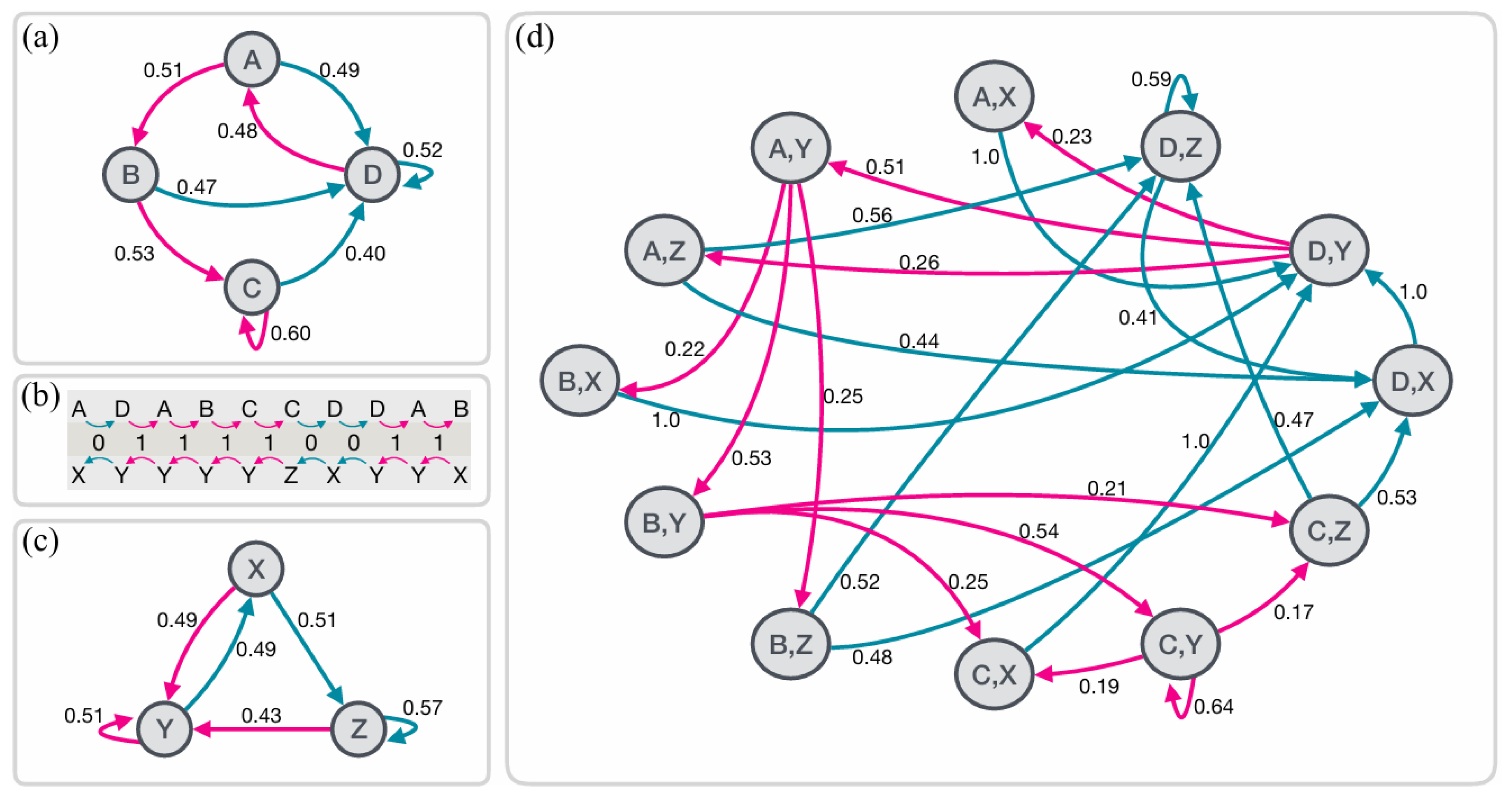
Appendix B.2. Spatial Distribution of Electrode Positions
Figure B2 presents the pairwise relationships between the X, Y, and Z coordinates of electrode positions, color-coded by brain lobe. The figure includes histograms displaying the distribution density, providing insights into the spatial distribution of electrodes across different brain regions.
Figure B2.
Spatial Distribution and Pairwise Relationships Among X, Y, Z Coordinates by Brain Lobe
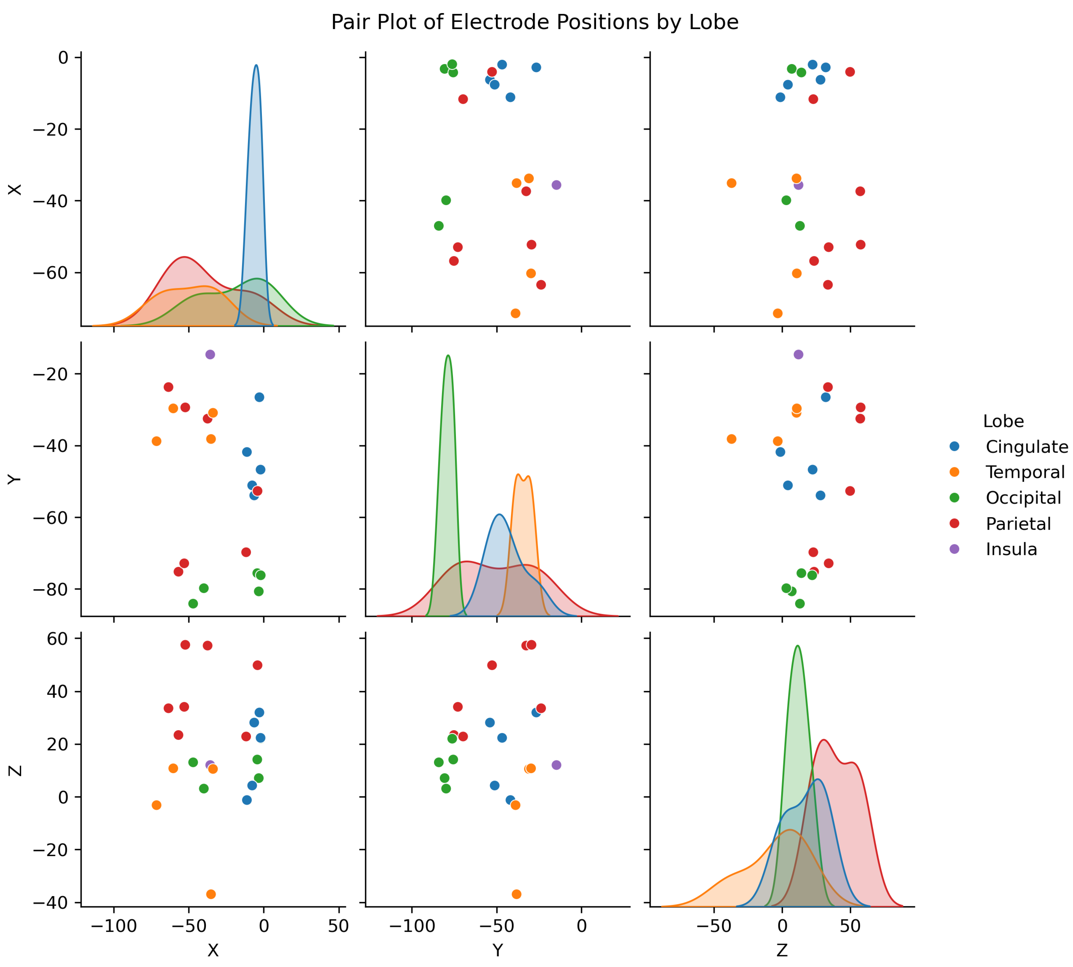
Appendix B.3. Lobe-Specific Activity Across Sleep States
In this section, the mean activity levels across various brain lobes for different participants are presented, highlighting how these activities vary across distinct sleep states. The detailed breakdown provided in (Figure B3) offers valuable insights into the lobe-specific contributions to overall brain activity during these states.
Figure B3.
Mean Activity Per Lobe Across Participants and Sleep States
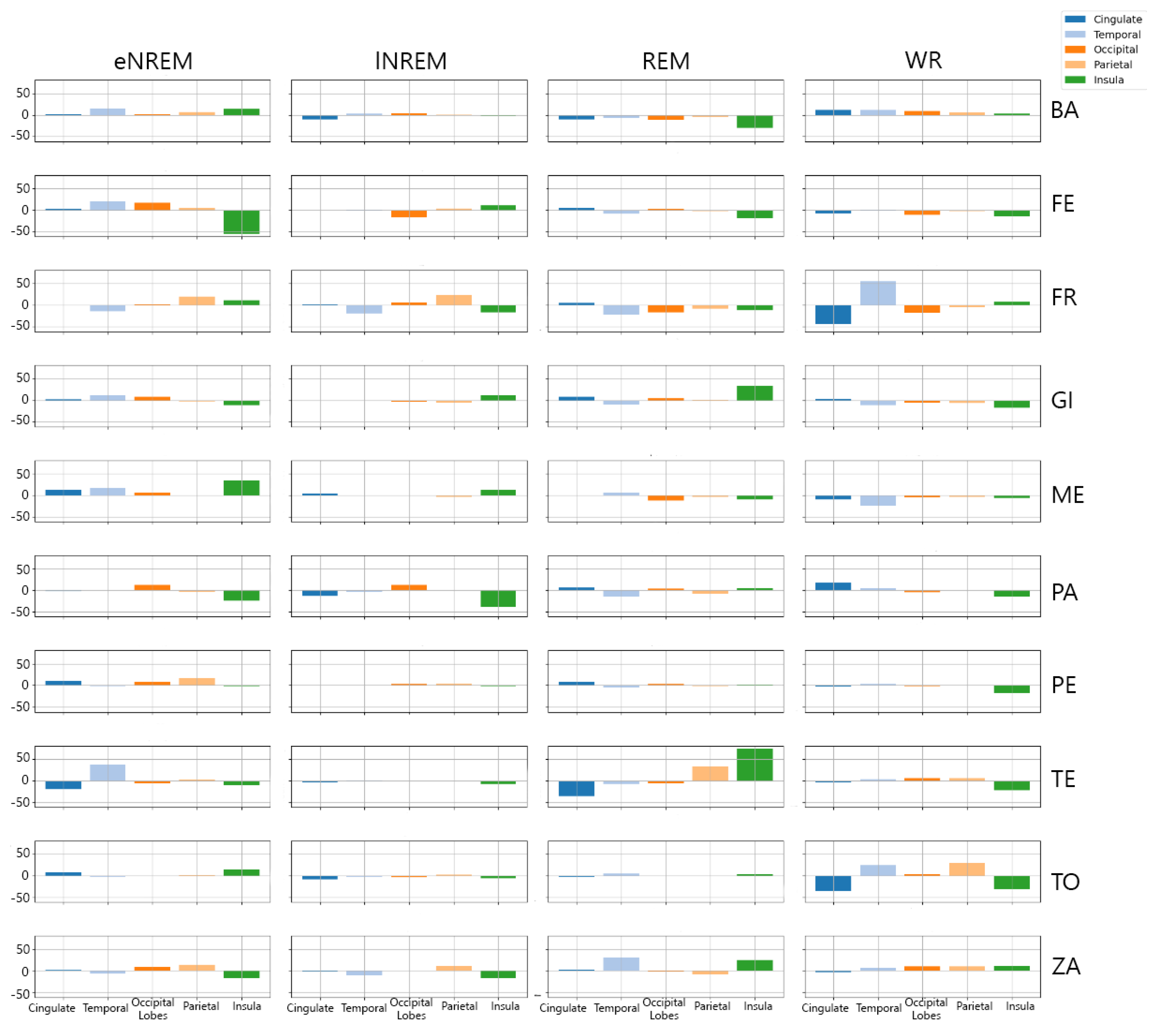
Appendix B.4. Participant-Specific Complexity Across Sleep States
The participant-specific profiles of Statistical Complexity and LZ Complexity across different sleep states, including eNREM, lNREM, REM, and wakeful rest (WR), are presented. Figure B4 illustrates the distinct patterns of complexity measures for each participant, revealing how these measures vary as participants transition through different states of sleep and wakefulness.
Figure B4.
Individual Complexity Profile
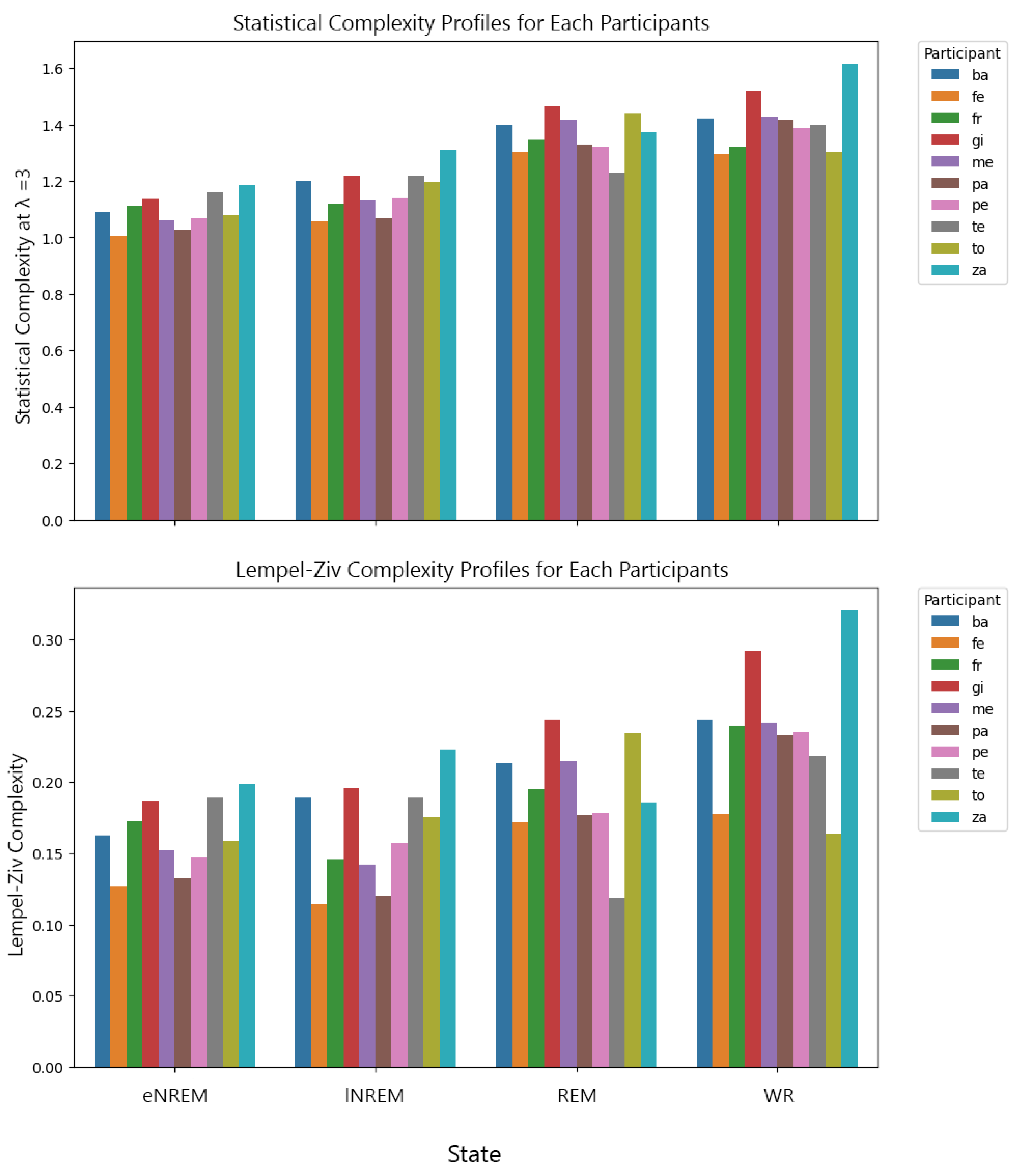
Appendix B.5. PCA-Based Clustering of Participants
Figure B5 delves into the clustering of participants based on their complexity profiles, using Principal Component Analysis (PCA). The plot visually represents how participants are grouped into distinct clusters, showcasing the similarities and differences in their Statistical Complexity and Lempel-Ziv Complexity measures across the various sleep states.
Figure B5.
Participant Clustering Based on Complexity Profiles
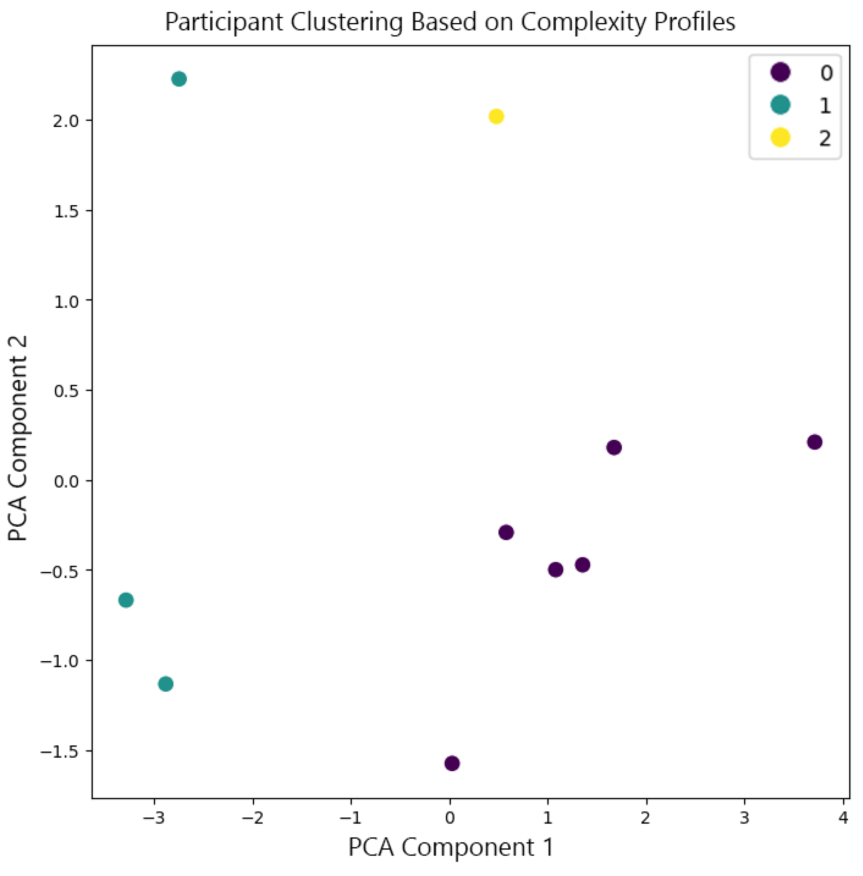
Appendix B.6. Distribution of Complexity Measures by Cluster
Figure B6 presents the distribution of Statistical Complexity and Lempel-Ziv Complexity measures for each sleep state across different clusters.
Figure B6.
Participants in Cluster 0 tend to have lower Statistical and Lempel-Ziv complexity measures across all sleep states, while those in Cluster 1 exhibit higher values for both measures. Cluster 2 consists of participants with outlier values, indicating unique complexity profiles that differ significantly from those in Clusters 0 and 1.
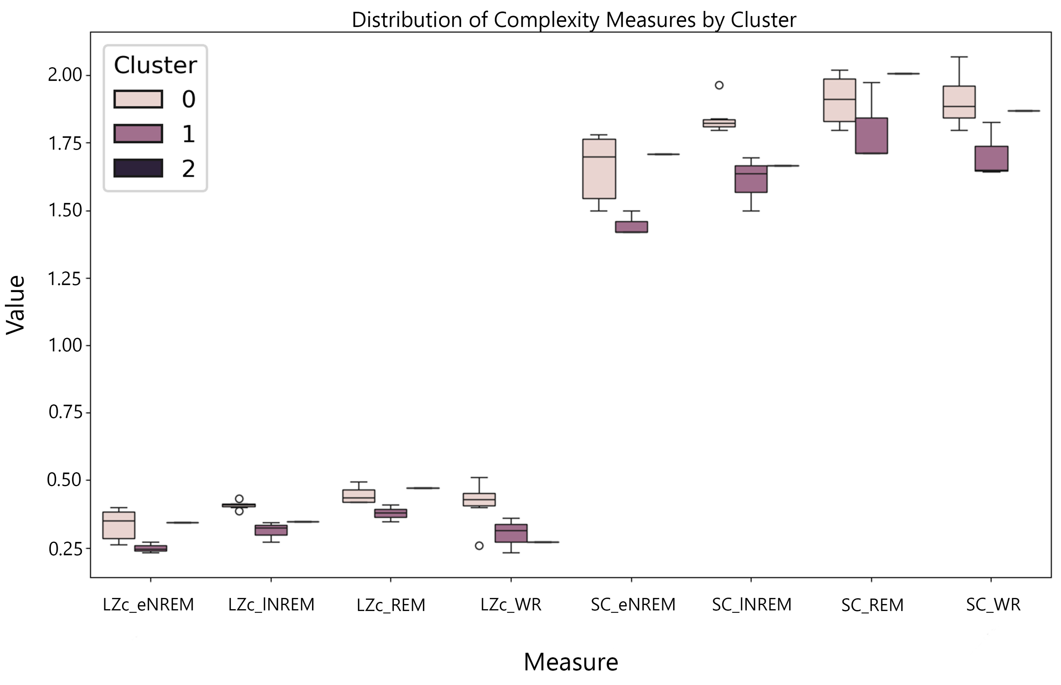
Appendix C Tables

Table C1.
t-Test Results for Statistical Complexity (SC) at Different Noise Levels and r-values
| r-Values | Noise Levels Comparison | t-statistic | p-value |
|---|---|---|---|
| 2.5 | 0.01 vs 0.05 | -0.065 | 0.950 |
| 2.6667 | 0.01 vs 0.05 | 0.304 | 0.769 |
| 2.8333 | 0.01 vs 0.05 | -0.120 | 0.907 |
| 3.0 | 0.01 vs 0.05 | 0.912 | 0.388 |
| 3.1667 | 0.01 vs 0.05 | -3.575 | 0.007 |
| 3.3333 | 0.01 vs 0.05 | -1.005 | 0.344 |
| 3.5 | 0.01 vs 0.05 | -2.827 | 0.022 |
| 3.6667 | 0.01 vs 0.05 | -47.866 | 0.000 |
| 3.8333 | 0.01 vs 0.05 | 0.787 | 0.454 |
| 4.0 | 0.01 vs 0.05 | 0.006 | 0.995 |
Results of t-tests conducted to compare statistical complexity (SC) at different noise levels (0.01 vs. 0.05) for various r-values.
- For and , the p-values are above 0.05, indicating that the differences in SC due to noise levels are not statistically significant. This suggests that noise has a minimal impact on SC for these r-values.
- For and , the p-values are below 0.05, indicating that the differences in SC due to noise levels are statistically significant. This means that for these r-values, noise significantly affects the statistical complexity of the system.
Table C2.
Effect of Increasing Noise Level and Segment Length on Complexity Measures and Lyapunov Exponent for Logistic Map with Selected r-values,
Table C2.
Effect of Increasing Noise Level and Segment Length on Complexity Measures and Lyapunov Exponent for Logistic Map with Selected r-values,
| r-Values | Noise Level | Segment Length | SC Mean | SC Std | LZ Mean | LZ Std | LE Mean | LE Std |
|---|---|---|---|---|---|---|---|---|
| 3.0 | 0.01 | 1500 | 1.881 | 0.049 | 0.870 | 0.050 | -0.005 | 0.002 |
| 3.0 | 0.01 | 2000 | 1.903 | 0.032 | 0.881 | 0.035 | -0.005 | 0.002 |
| 3.0 | 0.05 | 1500 | 1.400 | 0.300 | 0.995 | 0.009 | -0.062 | 0.008 |
| 3.0 | 0.05 | 2000 | 1.400 | 0.374 | 1.001 | 0.006 | -0.055 | 0.005 |
| 3.5 | 0.01 | 1500 | 1.005 | 0.011 | 0.284 | 0.006 | -0.423 | 0.016 |
| 3.5 | 0.01 | 2000 | 1.002 | 0.004 | 0.261 | 0.004 | -0.415 | 0.010 |
| 3.5 | 0.05 | 1500 | 1.007 | 0.009 | 0.286 | 0.005 | -0.058 | 0.016 |
| 3.5 | 0.05 | 2000 | 1.010 | 0.012 | 0.263 | 0.005 | -0.051 | 0.010 |
| 3.8333 | 0.01 | 1500 | 1.920 | 0.003 | 0.700 | 0.011 | -0.292 | 0.015 |
| 3.8333 | 0.01 | 2000 | 1.919 | 0.001 | 0.682 | 0.008 | -0.296 | 0.020 |
| 3.8333 | 0.05 | 1500 | 1.920 | 0.001 | 0.702 | 0.007 | 0.201 | 0.017 |
| 3.8333 | 0.05 | 2000 | 1.919 | 0.001 | 0.681 | 0.004 | 0.213 | 0.016 |
Note: Summary of SC, LZc, and LE for selected r-values, noise levels, and segment lengths. Statistical complexity generally decreases with increasing segment length, especially for lower values of r, while LZc tends to remain stable around 1 for different noise levels and segment lengths. Higher noise levels tend to result in more variability in SC values, indicating that noise impacts the measured complexity of the system.
References
- Strogatz, S. Nonlinear Dynamics And Chaos: With Applications To Physics, Biology, Chemistry, And Engineering (Studies in Nonlinearity). CRC Press 2000, 2, 1–532. [Google Scholar] [CrossRef]
- Devaney, R. An introduction to chaotic dynamical systems; CRC press, 2018. [CrossRef]
- Lempel, A.; Ziv, J. On the complexity of finite sequences. IEEE Transactions on information theory 1976, 22, 75–81. [Google Scholar] [CrossRef]
- Muñoz, R.N.; Leung, A.; Zecevik, A.; Pollock, F.A.; Cohen, D.; Van Swinderen, B.; Tsuchiya, N.; Modi, K. General anesthesia reduces complexity and temporal asymmetry of the informational structures derived from neural recordings in Drosophila. Physical Review Research 2020, 2, 023219. [Google Scholar] [CrossRef]
- Pincus, S.M. Approximate entropy as a measure of system complexity. Proceedings of the national academy of sciences 1991, 88, 2297–2301. [Google Scholar] [CrossRef] [PubMed]
- Shen, A.; Uspensky, V.A.; Vereshchagin, N. Kolmogorov Complexity and Algorithmic Randomness; Vol. 220, Mathematical Surveys and Monographs, American Mathematical Society, 2017. [CrossRef]
- Sarasso, S.; Casali, A.G.; Casarotto, S.; others. Consciousness and complexity: a consilience of evidence. Neuroscience of Consciousness 2021, 2021, niab023. [Google Scholar] [CrossRef]
- Zhang, X.S.; Roy, R.J.; Jensen, E.W. EEG complexity as a measure of depth of anesthesia for patients. IEEE transactions on biomedical engineering 2001, 48, 1424–1433. [Google Scholar] [CrossRef]
- Burioka, N.; Miyata, M.; Cornélissen, G.; Halberg, F.; Takeshima, T.; Kaplan, D.T.; Suyama, H.; Endo, M.; Maegaki, Y.; Nomura, T.; others. Approximate entropy in the electroencephalogram during wake and sleep. Clinical EEG and neuroscience 2005, 36, 21–24. [Google Scholar] [CrossRef]
- Casali, A.G.; Gosseries, O.; Rosanova, M.; Boly, M.; Sarasso, S.; Casali, K.R.; Casarotto, S.; Bruno, M.A.; Laureys, S.; Tononi, G.; others. A theoretically based index of consciousness independent of sensory processing and behavior. Science translational medicine 2013, 5, 198ra105–198ra105. [Google Scholar] [CrossRef]
- Schartner, M.; Seth, A.; Noirhomme, Q.; Boly, M.; Bruno, M.A.; Laureys, S.; Barrett, A. Complexity of multi-dimensional spontaneous EEG decreases during propofol induced general anaesthesia. PloS one 2015, 10, e0133532. [Google Scholar] [CrossRef]
- Andrillon, T.; Poulsen, A.T.; Hansen, L.K.; Léger, D.; Kouider, S. Neural markers of responsiveness to the environment in human sleep. Journal of Neuroscience 2016, 36, 6583–6596. [Google Scholar] [CrossRef]
- Schartner, M.M.; Pigorini, A.; Gibbs, S.A.; Arnulfo, G.; Sarasso, S.; Barnett, L.; Nobili, L.; Massimini, M.; Seth, A.K.; Barrett, A.B. Global and local complexity of intracranial EEG decreases during NREM sleep. Neuroscience of consciousness 2017, 2017, niw022. [Google Scholar] [CrossRef] [PubMed]
- Carhart-Harris, R.L.; Leech, R.; Hellyer, P.J.; Shanahan, M.; Feilding, A.; Tagliazucchi, E.; Chialvo, D.R.; Nutt, D. The entropic brain: a theory of conscious states informed by neuroimaging research with psychedelic drugs. Frontiers in human neuroscience 2014, 8, 20. [Google Scholar] [CrossRef] [PubMed]
- Schartner, M.M.; Carhart-Harris, R.L.; Barrett, A.B.; Seth, A.K.; Muthukumaraswamy, S.D. Increased spontaneous MEG signal diversity for psychoactive doses of ketamine, LSD and psilocybin. Scientific Reports 2017, 7, 46421. [Google Scholar] [CrossRef] [PubMed]
- Mediano, P.A.M.; Rosas, F.E.; Timmermann, C.; Roseman, L.; Nutt, D.J.; Feilding, A.; Kaelen, M.; Kringelbach, M.L.; Barrett, A.B.; Seth, A.K.; Muthukumaraswamy, S.; Bor, D.; Carhart-Harris, R.L. Effects of External Stimulation on Psychedelic State Neurodynamics. ACS Chemical Neuroscience 2024, 15, 462–471. [Google Scholar] [CrossRef]
- Ruffini, G.; Damiani, G.; Lozano-Soldevilla, D.; Deco, N.; Rosas, F.E.; Kiani, N.A.; Ponce-Alvarez, A.; Kringelbach, M.L.; Carhart-Harris, R.; Deco, G. LSD-induced increase of Ising temperature and algorithmic complexity of brain dynamics. PLoS Comput Biol 2023, 19, e1010811. [Google Scholar] [CrossRef]
- Tononi, G. An information integration theory of consciousness. BMC Neuroscience 2004, 5, 42. [Google Scholar] [CrossRef]
- Oizumi, M.; Albantakis, L.; Tononi, G. From the phenomenology to the mechanisms of consciousness: Integrated Information Theory 3.0. PLoS Computational Biology 2014, 10, e1003588. [Google Scholar] [CrossRef]
- Tononi, G.; Koch, C. The Integrated Information Theory of Consciousness: An Updated Account. Archives Italiennes de Biologie 2015, 153, 205–235. [Google Scholar] [CrossRef]
- Barrett, A.B.; Seth, A.K. Practical measures of integrated information for time-series data. PLoS computational biology 2011, 7, e1001052. [Google Scholar] [CrossRef]
- Bayne, T. On the axiomatic foundations of the integrated information theory of consciousness. Neuroscience of consciousness 2018, 2018, niy007. [Google Scholar] [CrossRef]
- Bau, H.H.; Shachmurove, Y. Process unpredictability in deterministic systems. Indeterminacy: The Mapped, the Navigable, and the Uncharted 2009, 1, 123–145. [Google Scholar] [CrossRef]
- Li, W. Random texts exhibit Zipf’s-law-like word frequency distribution. IEEE Transactions on information theory 1992, 38, 1842–1845. [Google Scholar] [CrossRef]
- May, R.M. Simple mathematical models with very complicated dynamics. Nature 1976, 261, 459–467. [Google Scholar] [CrossRef] [PubMed]
- Brown, M.D. Chaos and nonlinear dynamics: An introduction for scientists and engineers, 1996.
- Seth, A.K. Causal connectivity of evolved neural networks during behavior. Network: Computation in Neural Systems 2005, 16, 35–54. [Google Scholar] [CrossRef]
- Barnett, L.; Seth, A.K. The MVGC multivariate Granger causality toolbox: a new approach to Granger-causal inference. Journal of neuroscience methods 2014, 223, 50–68. [Google Scholar] [CrossRef]
- Ziv, J.; Lempel, A. A universal algorithm for sequential data compression. IEEE Transactions on information theory 1977, 23, 337–343. [Google Scholar] [CrossRef]
- Richman, J.S.; Moorman, J.R. Physiological time-series analysis using approximate entropy and sample entropy. American Journal of Physiology-Heart and Circulatory Physiology 2000, 278, H2039–H2049. [Google Scholar] [CrossRef]
- Crutchfield, J.P.; Young, K. Inferring statistical complexity. Physical review letters 1989, 63 2, 105–108. [Google Scholar] [CrossRef]
- Starkey, J.; Carhart-Harris, R.; Pigorini, A.; Nobili, L.; Barrett, A. Statistical diversity distinguishes global states of consciousness. bioRxiv 2023, pp. 2023–12. [CrossRef]
- Atmanspacher, H. On macrostates in complex multi-scale systems. Entropy 2016, 18, 426. [Google Scholar] [CrossRef]
- Ziv, J.; Lempel, A. Compression of individual sequences via variable-rate coding. IEEE transactions on Information Theory 1978, 24, 530–536. [Google Scholar] [CrossRef]
- Radhakrishnan, N.; Gangadhar, B. Estimating regularity in epileptic seizure time-series data. IEEE engineering in medicine and biology magazine 1998, 17, 89–94. [Google Scholar] [CrossRef] [PubMed]
- Gusev, V.; Nemytikova, L.; Chuzhanova, N. On the complexity measures of genetic sequences. Bioinformatics 1999, 15, 994–999. [Google Scholar] [CrossRef] [PubMed]
- Zhang, X.S.; Zhu, Y.S.; Thakor, N.V.; Wang, Z.Z. Detecting ventricular tachycardia and fibrillation by complexity measure. IEEE Transactions on biomedical engineering 1999, 46, 548–555. [Google Scholar] [CrossRef]
- Aboy, M.; Hornero, R.; Abásolo, D.; Álvarez, D. Interpretation of the Lempel-Ziv complexity measure in the context of biomedical signal analysis. IEEE transactions on biomedical engineering 2006, 53, 2282–2288. [Google Scholar] [CrossRef]
- Mitchell, M. Complexity: A Guided Tour; Oxford University Press, 2009.
- Freeman, W. Neurodynamics: an exploration in mesoscopic brain dynamics; Springer Science & Business Media, 2000. [CrossRef]
- Tononi, G.; Edelman, G.M. Consciousness and complexity. Science 1998, 282, 1846–1851. [Google Scholar] [CrossRef]
- Ebeling, W.; others. Partition-Based Entropies of Deterministic and Stochastic Maps. ResearchGate 1999. [Google Scholar]
- Benedetto, D.; Caglioti, E.; Loreto, V. Language Trees and Zipping. Physical Review Letters 2002, 88, 048702. [Google Scholar] [CrossRef]
- Balasubramanian, K.; Nair, S.S.; Nagaraj, N. Classification of periodic, chaotic and random sequences using approximate entropy and Lempel–Ziv complexity measures. Pramana 2015, 84, 365–372. [Google Scholar] [CrossRef]
- Thelen, E. Dynamic systems theory and the complexity of change. Psychoanalytic dialogues 2005, 15, 255–283. [Google Scholar] [CrossRef]
- Smith, L.B. Cognition as a dynamic system: Principles from embodiment. Developmental Review 2005, 25, 278–298. [Google Scholar] [CrossRef]
- Spencer, J.P.; Clearfield, M.; Corbetta, D.; Ulrich, B.; Buchanan, P.; Schöner, G. Moving toward a grand theory of development: In memory of Esther Thelen. Child Development 2006, 77, 1521–1538. [Google Scholar] [CrossRef]
- Hill, S.; Tononi, G. Modeling sleep and wakefulness in the thalamocortical system. Journal of neurophysiology 2005, 93, 1671–1698. [Google Scholar] [CrossRef] [PubMed]
- Massimini, M.; Ferrarelli, F.; Huber, R.; Esser, S.K.; Singh, H.; Tononi, G. Breakdown of cortical effective connectivity during sleep. Science 2005, 309, 2228–2232. [Google Scholar] [CrossRef] [PubMed]
- Toker, D.; Pappas, I.; Lendner, J.D.; Frohlich, J.; Mateos, D.M.; Muthukumaraswamy, S.; Carhart-Harris, R.; Paff, M.; Vespa, P.M.; Monti, M.M.; Sommer, F.T.; Knight, R.T.; D’Esposito, M. Consciousness is supported by near-critical slow cortical electrodynamics. Proceedings of the National Academy of Sciences 2022, 119, e2024455119. [Google Scholar] [CrossRef] [PubMed]
- Bak, P.; Tang, C.; Wiesenfeld, K. Self-organized criticality: An explanation of the 1/f noise. Physical Review Letters 1987, 59, 381–384. [Google Scholar] [CrossRef]
- Langton, C.G. Computation at the edge of chaos: Phase transitions and emergent computation. Physica D: Nonlinear Phenomena 1990, 42, 12–37. [Google Scholar] [CrossRef]
- Benettin, G.; Galgani, L.; Giorgilli, A.; Strelcyn, J.M. Lyapunov characteristic exponents for smooth dynamical systems and for Hamiltonian systems; a method for computing all of them. Part 1: Theory. Meccanica 1980, 15, 9–20. [Google Scholar] [CrossRef]
- Wilkinson, A. What are Lyapunov exponents, and why are they interesting? Bulletin of the American Mathematical Society 2017, 54, 79–105. [Google Scholar] [CrossRef]
- Gourévitch, B.; Bouquin-Jeannès, R.L.; Faucon, G. Linear and nonlinear causality between signals: methods, examples and neurophysiological applications. Biological cybernetics 2006, 95, 349–369. [Google Scholar] [CrossRef]
- Seth, A.K.; Barrett, A.B.; Barnett, L. Granger causality analysis in neuroscience and neuroimaging. Journal of Neuroscience 2015, 35, 3293–3297. [Google Scholar] [CrossRef]
- Shalizi, C.R.; Klinkner, K.L. Consistency under sampling of exponential random graph models. Proceedings of the 20th Conference on Uncertainty in Artificial Intelligence (UAI’04). AUAI Press, 2004, pp. 504–511. [CrossRef]
- Gagniuc, P.A. Markov chains: from theory to implementation and experimentation; John Wiley & Sons, 2017. [CrossRef]
- Crutchfield, J.P.; Ellison, C.J.; Mahoney, J.R. Time’s Barbed Arrow: Irreversibility, Crypticity, and Stored Information. Physical Review Letters 2009, 103, 094101. [Google Scholar] [CrossRef]
- Bloem, P.; Mota, F.; de Rooij, S.; Antunes, L.; Adriaans, P. A safe approximation for Kolmogorov complexity. International conference on algorithmic learning theory. Springer, 2014, pp. 336–350. [CrossRef]
- Vitányi, P.M. How incomputable is Kolmogorov complexity? Entropy 2020, 22, 408. [Google Scholar] [CrossRef]
- von Wegner, F.; Tagliazucchi, E.; Laufs, H. Information-theoretical analysis of resting state EEG microstate sequences — non-Markovianity, nonstationarity and periodicities. NeuroImage 2017, 158, 99–111. [Google Scholar] [CrossRef] [PubMed]
- Cohen, J. Statistical Power Analysis for the Behavioral Sciences, 2nd ed.; Routledge: New York, 1988. [Google Scholar]
- Carhart-Harris, R.L. The entropic brain – Revisited. Neuropharmacology 2018, 142, 167–178. [Google Scholar] [CrossRef] [PubMed]
- González, J.; Cavelli, M.; Mondino, A.; others. Decreased electrocortical temporal complexity distinguishes sleep from wakefulness. Scientific Reports 2019, 9, 18457. [Google Scholar] [CrossRef] [PubMed]
- Beggs, J.M.; Timme, N. Criticality in neural systems. Nature Reviews Neuroscience 2012, 13, 49–58. [Google Scholar] [CrossRef]
- Tagliazucchi, E.; others. Complexity and coherence: Lost and found in the transition between wakefulness and sleep. NeuroImage 2013, 64, 385–395. [Google Scholar] [CrossRef]
- Goldberger, A.L.; Amaral, L.A.; Hausdorff, J.M.; Ivanov, P.C.; Peng, C.K.; Stanley, H.E. Fractal dynamics in physiology: Alterations with disease and aging. Proceedings of the National Academy of Sciences 2002, 99, 2466–2472. [Google Scholar] [CrossRef]
- Sporns, O. Neural complexity and structural connectivity. Current Opinion in Neurobiology 2013, 23, 162–171. [Google Scholar] [CrossRef]
| 1 | The ’Hilbert Transform’ is used to generate an analytic signal from the real-valued time series, allowing for the extraction of the instantaneous amplitude, which is then used for binarization. |
| 2 | In this context, ’future’ refers to the subsequent observations from the present state. Although using the next single state may perform better on random data, the decision to use the next states for other models was made to capture more temporal correlations. However, future exploration will focus on considering the next single binary state across all models. |
| 3 | Simonsohn’s two-lines test is a statistical method used to determine whether there is a significant change in slope in a dataset, particularly when hypothesizing a U-shaped or inverted U-shaped relationship. |
Figure 1.
Statistical Complexity (SC) calculation example (for and ). a) demonstrates the segmentation of a binary string into substrings of length 2, followed by refinement based on the distribution of successor states. Substrings with highly similar successor distributions are combined into the same refined state. For example, ’01’ and ’11’ are grouped together as they both predict the next state with similar certainty (difference of 0.00, within the threshold). This concept is further illustrated in b), where the state distributions and transitions clarify the grouping process [32].
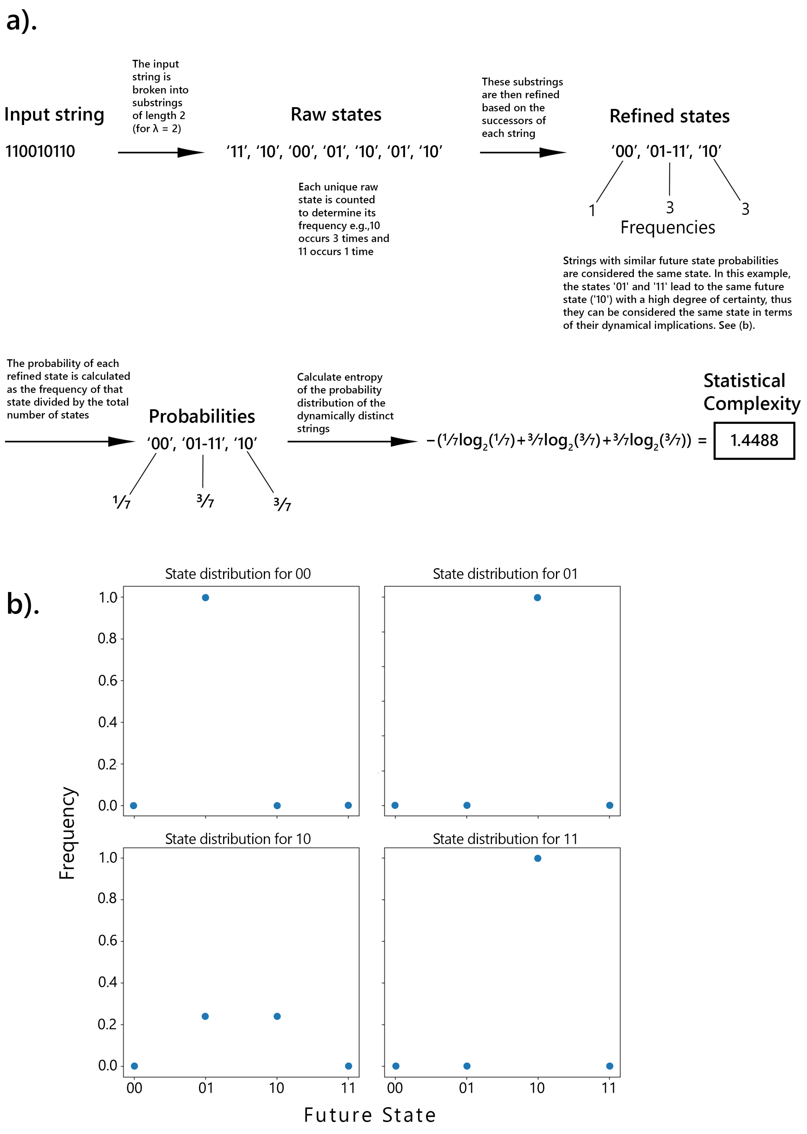
Figure 2.
Two classes of complexity measures: monotonic and convex. Monotonic complexity, related to syntactic information, increases with randomness. In contrast, convex complexity, associated with pragmatic information, peaks at intermediate levels of randomness and diminishes towards zero for both complete order and complete randomness, highlighting its dependence on meaningful structure [33].
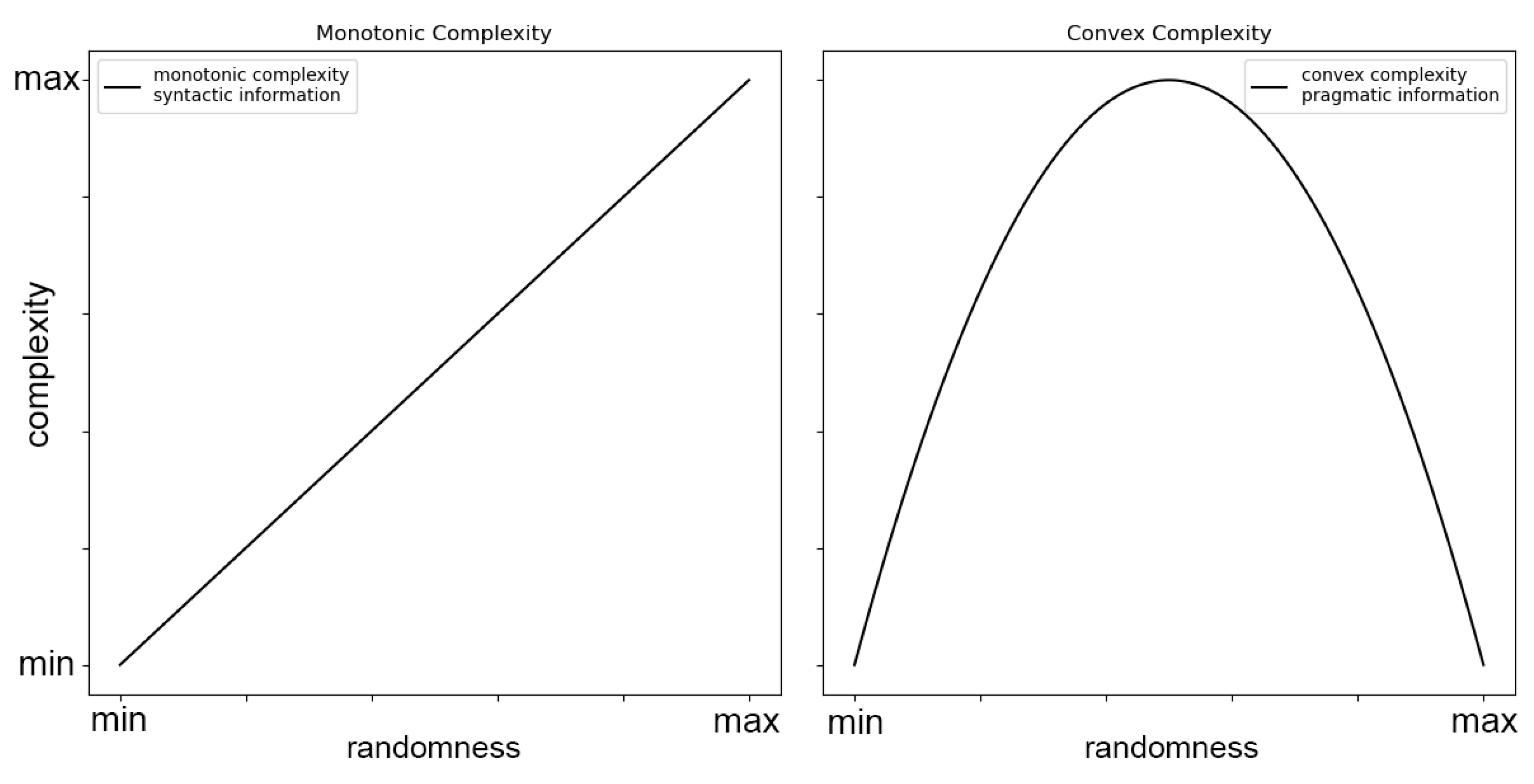
Figure 3.
Lempel-Ziv Complexity Computation Algorithm. From the start of the string, each character is analyzed and added to a "search string." If this search string is identical to a previously discovered string, the next character in the sequence is added to the search string. If it is not, the search string is added to the list of previously discovered strings, and then the search string is "reset" to an empty string before moving on to the next character in the sequence. This process repeats until the end of the sequence is reached.
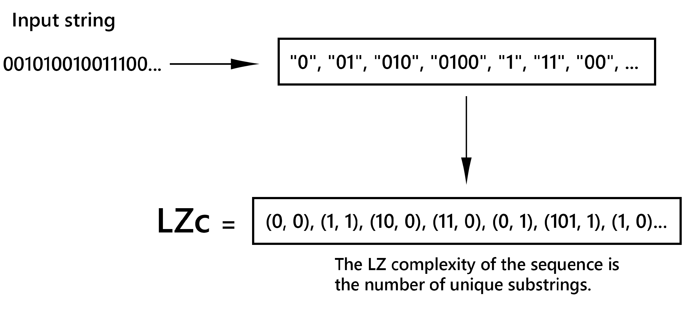
Figure 4.
Bifurcation Diagram of the Logistic Map. The attractor values for each value of r are shown along the corresponding vertical line. This diagram illustrates the transition from stable, periodic behavior to chaotic dynamics as r increases, showcasing the complex behavior inherent in the logistic map as a nonlinear system.
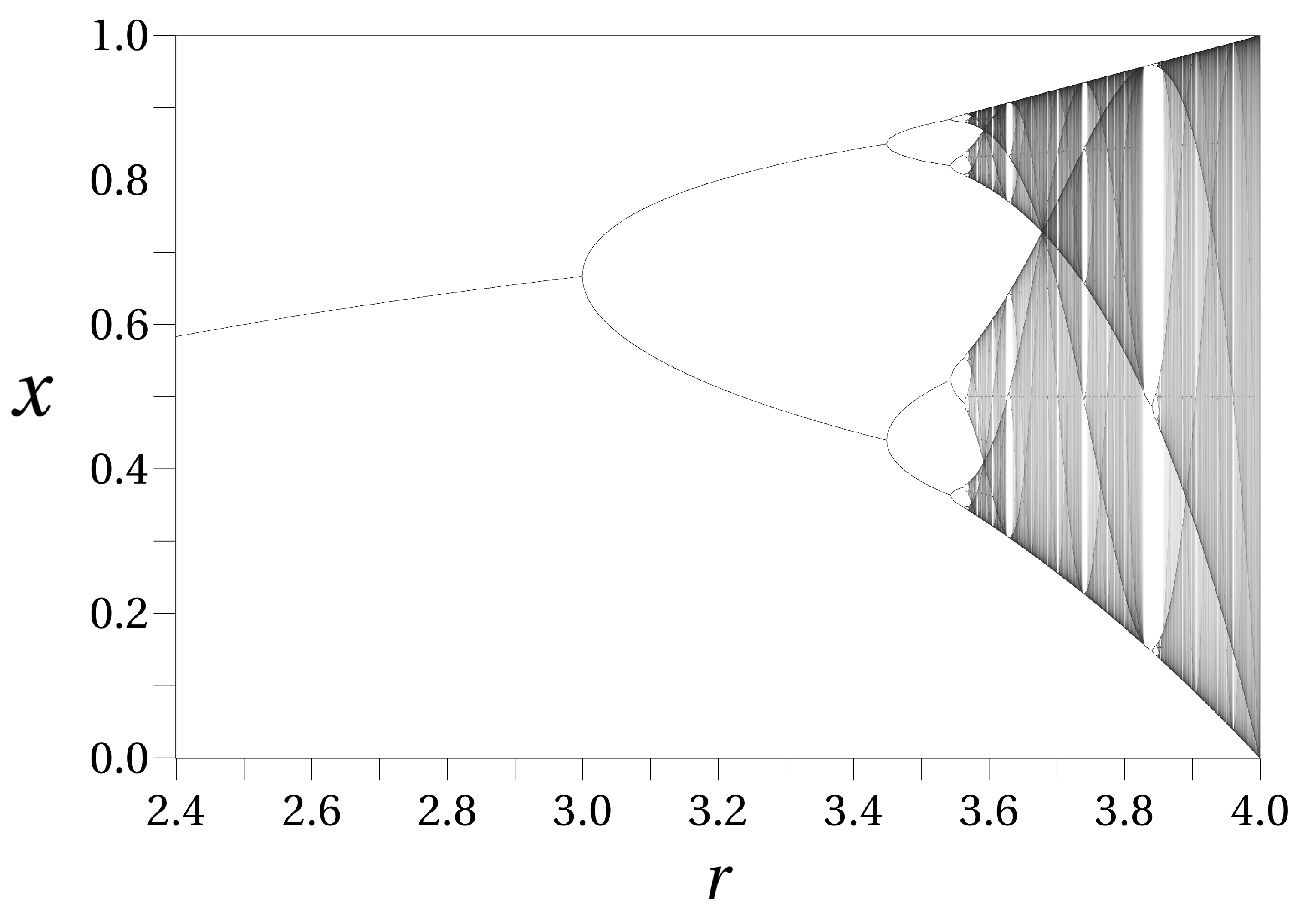
Figure 5.
Spatial distribution of electrode positions in MNI coordinate space, highlighting their clustering within specific brain areas.
Figure 5.
Spatial distribution of electrode positions in MNI coordinate space, highlighting their clustering within specific brain areas.
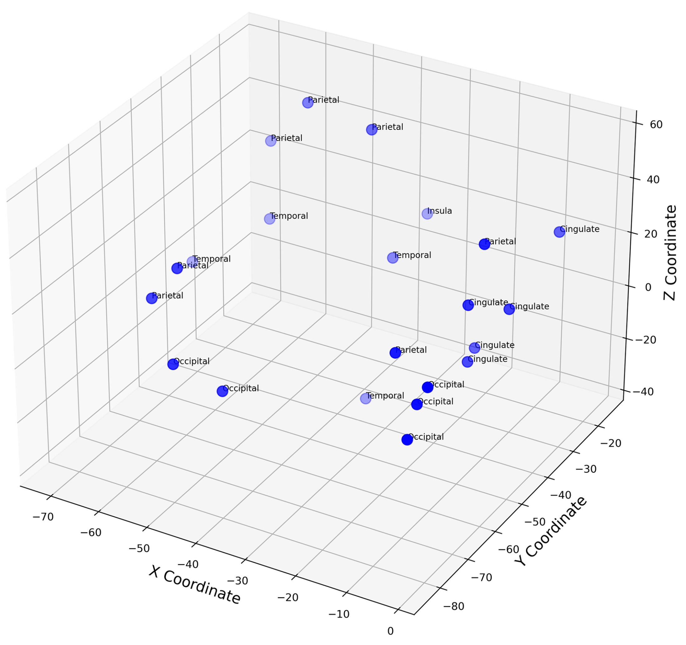
Figure 6.
Complexity measures vs sequence length a). Statistical Complexity for and : Average SC values decrease as sequence length increases. b). LZc is relatively stable across varying sequence lengths. c). Mean SC and LZc with varying sequence length
Figure 6.
Complexity measures vs sequence length a). Statistical Complexity for and : Average SC values decrease as sequence length increases. b). LZc is relatively stable across varying sequence lengths. c). Mean SC and LZc with varying sequence length
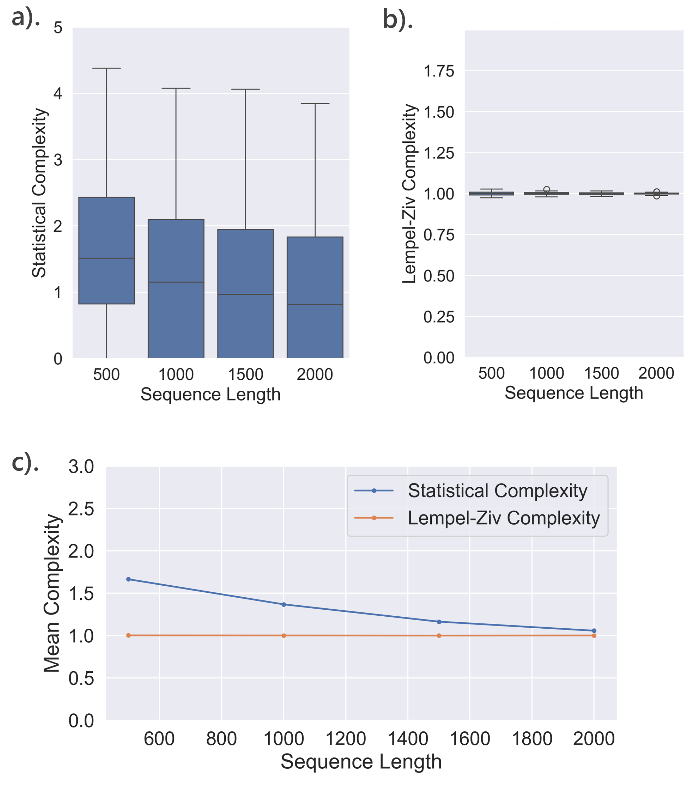
Figure 7.
Impact of ’Future’ State Definition on Statistical Complexity Across Sequence Lengths. In a), the future is defined as the next state, while in b), it is defined as the immediate next binary state. Each plot compares different memory lengths () and tolerance levels (), showing that complexity generally decreases with increasing sequence length, with more significant reductions at higher tolerance levels. The comparison reveals that predicting a single future state generally requires less memory, resulting in lower complexity, whereas predicting multiple future states involves greater structural richness, reflected in higher initial complexity values.
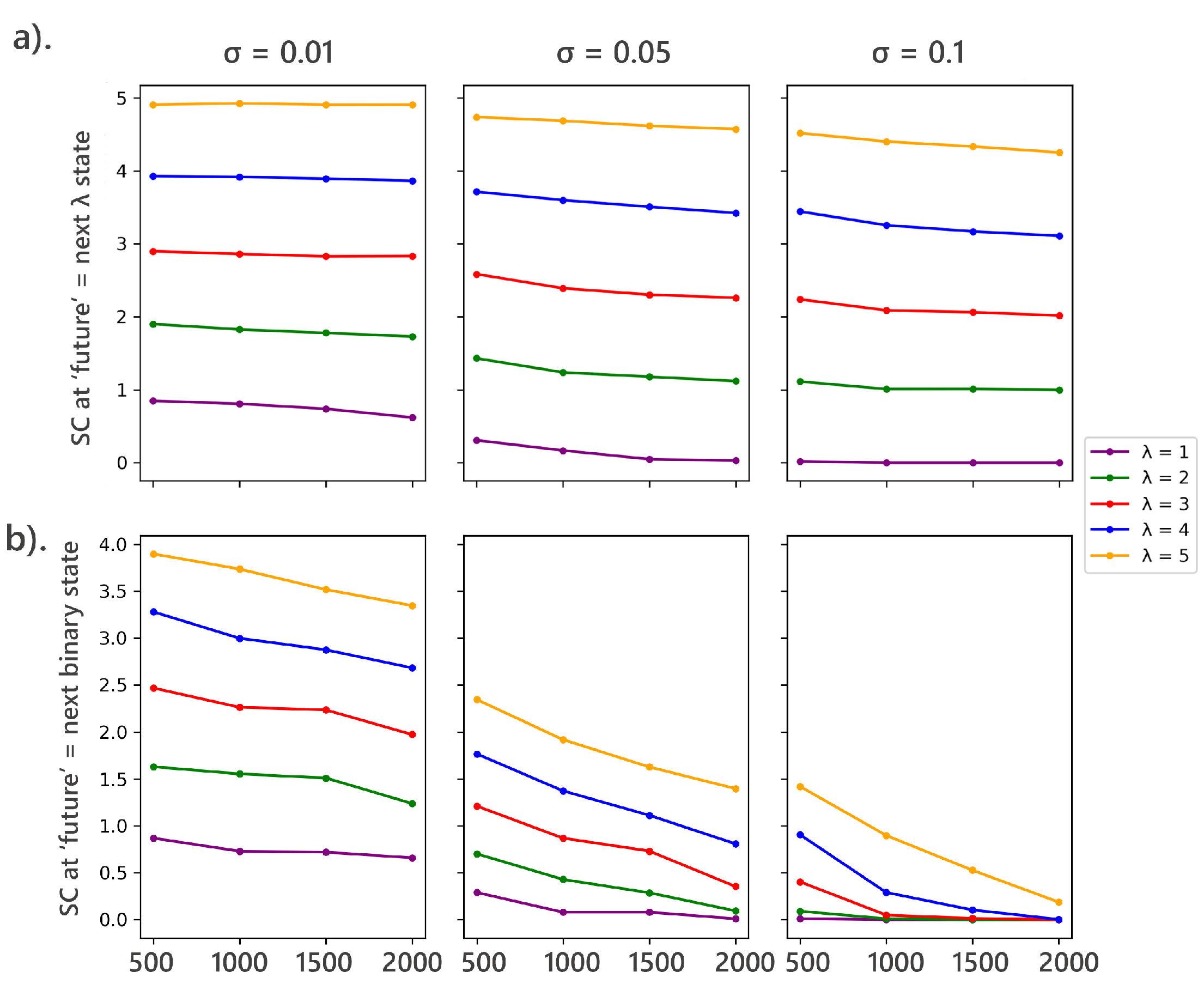
Figure 8.
Comparison of Complexity Measures and Lyapunov Exponent Across r-Values for the Logistic Map. The plots illustrate the behavior of various complexity measures—Statistical Complexity, Lempel-Ziv Complexity, Kolmogorov Complexity, and Approximate Entropy—along with the Lyapunov Exponent as functions of the r-value in the logistic map. Panel (a) shows the normalized values of Statistical Complexity, Lempel-Ziv Complexity, and the Lyapunov Exponent. Panel (b) includes additional comparisons with Kolmogorov Complexity and Approximate Entropy. The observed trends highlight the onset and development of chaos as r increases, with different complexity measures capturing distinct aspects of the system’s dynamics.
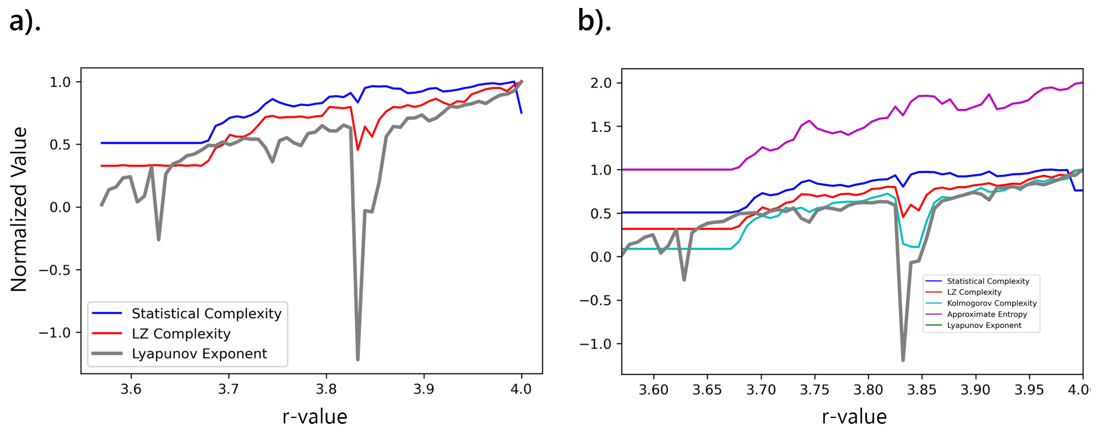
Figure 9.
95% confidence intervals for the averaged values of a) Statistical Complexity and b) Lempel-Ziv Complexity across different dynamical regimes of the logistic map: Periodic (), Weak Chaos (), Strong Chaos (), and Random. Statistical Complexity is more pronounced in the periodic and weak chaos regimes, capturing the underlying structure and predictability of the sequences. In contrast, Lempel-Ziv Complexity increases in strong chaos and random sequences, reflecting the higher levels of randomness and reduced compressibility in these behaviors c). Correlation between LZc and SC across Different Bifurcation Parameters. The strength and direction of the correlation vary between the regimes. Negative correlations are observed across all regimes, suggesting a potential inverse relationship between LZc and SC, with statistically significant p-values in most cases. The periodic and weak chaos regimes exhibit moderate negative correlations, while the strong chaos and random regimes show weaker correlations.
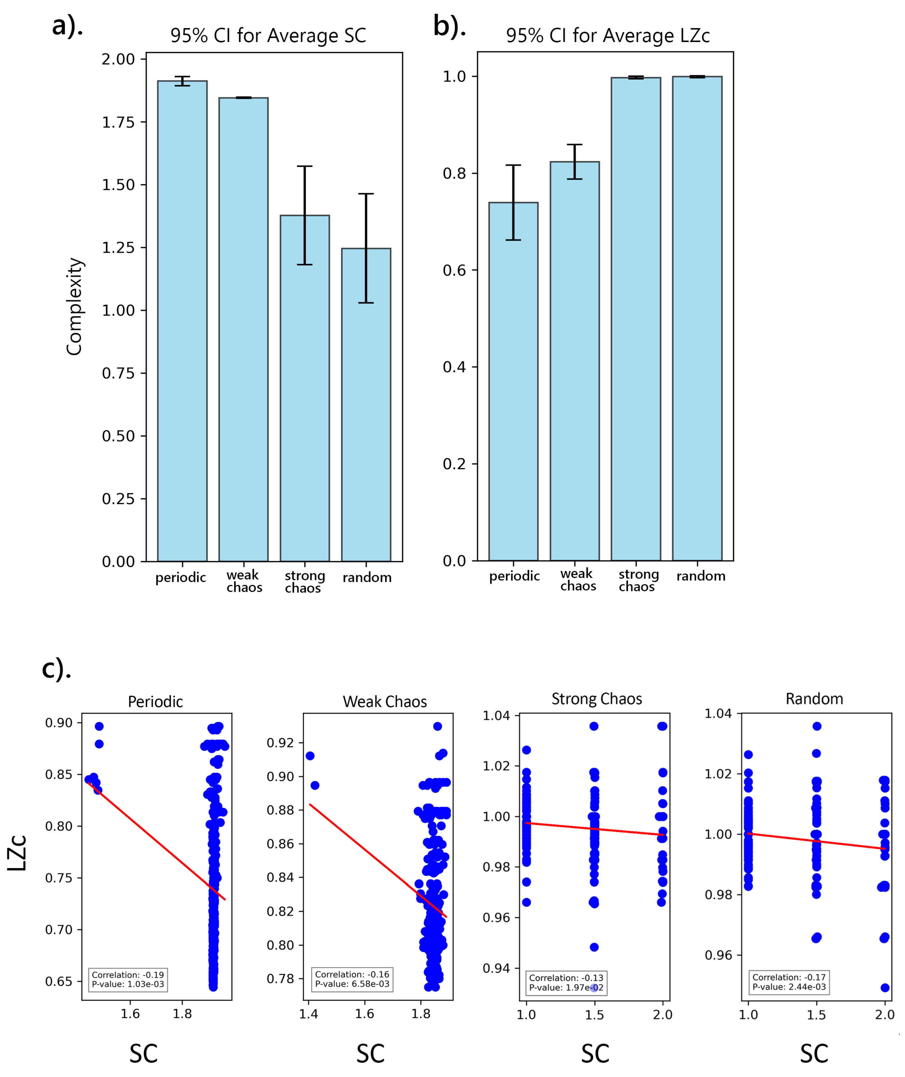
Figure 10.
Phase-space plots depicting the attractor structures of the logistic map for various values of the parameter r and different noise levels (0, 0.01, 0.05, and 0.1). The plots illustrate how the introduction of noise affects the system behavior, leading to a dispersion of the attractor points and increasing complexity. As the noise level increases, the attractors become more diffuse, indicating a transition from deterministic chaos to stochastic behavior, particularly evident in highly chaotic regions such as .
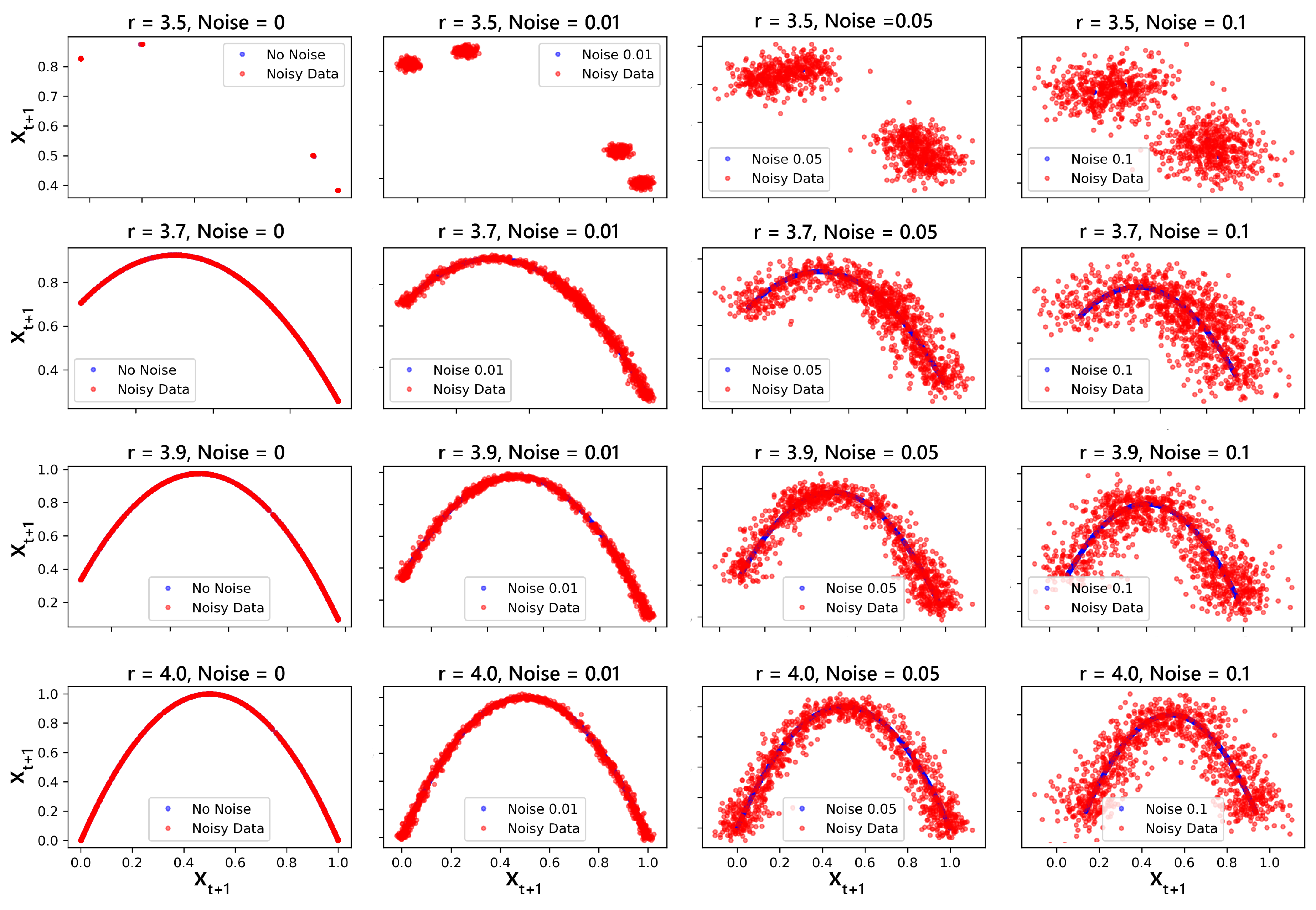
Figure 11.
Complexity vs Lyapunov Exponent for Logistic Map, Segment Length=1000.
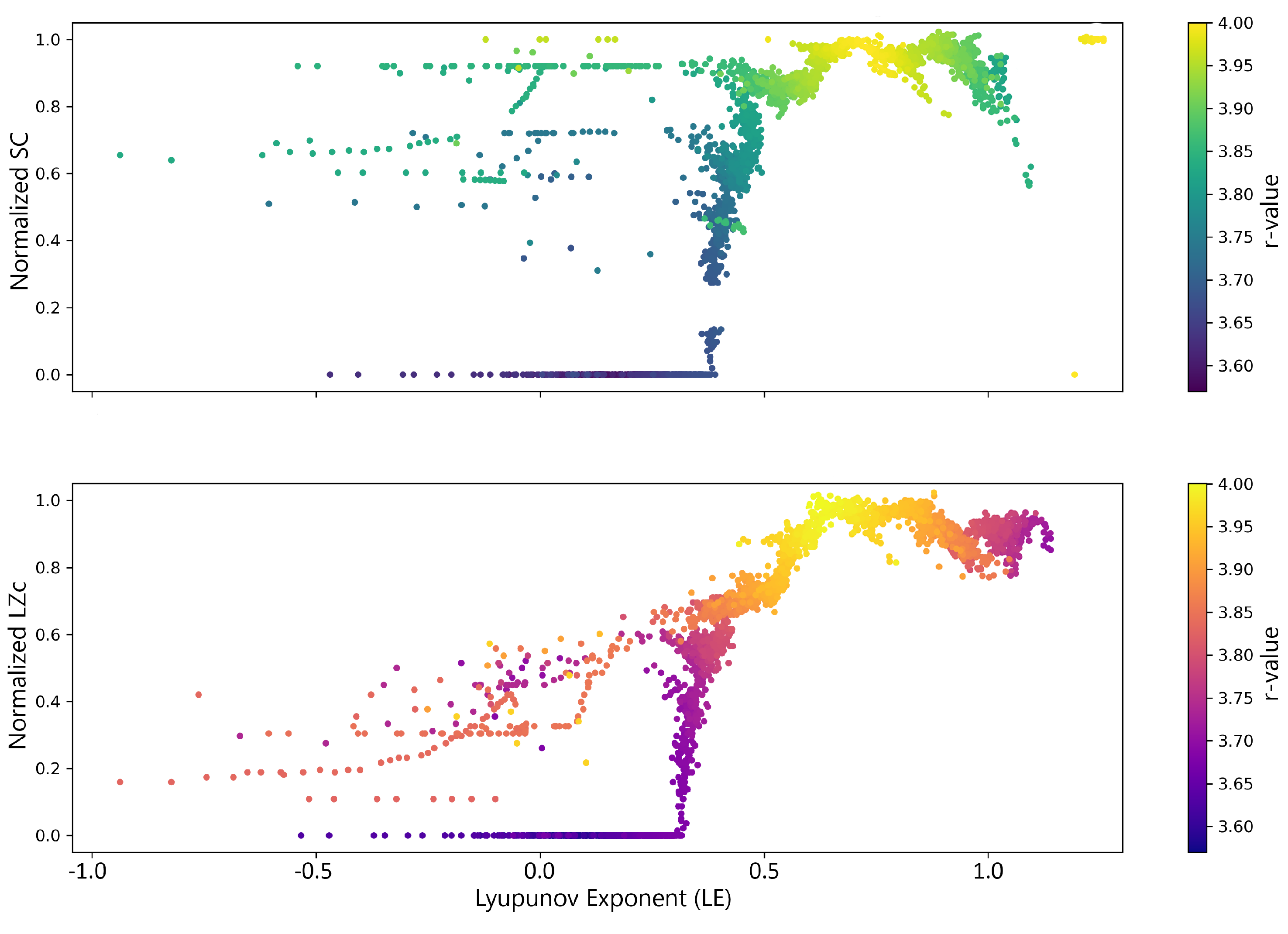
Figure 12.
Analysis of Complexity Measures with Lyapunov Exponent Using Simonsohn’s Two-Lines Test: (a) and (b) illustrate the relationship between Lempel-Ziv complexity and statistical complexity and the Lyapunov exponent in logistic map dynamics. Simonsohn’s two-lines test identifies a breakpoint in both cases. In a), the Lempel-Ziv complexity shows a consistent slight positive trend across the identified breakpoint. In b), the statistical complexity exhibits a change from a moderate positive relationship to a steep negative relationship at the breakpoint, suggesting a transition in the system behavior as chaoticity increases.
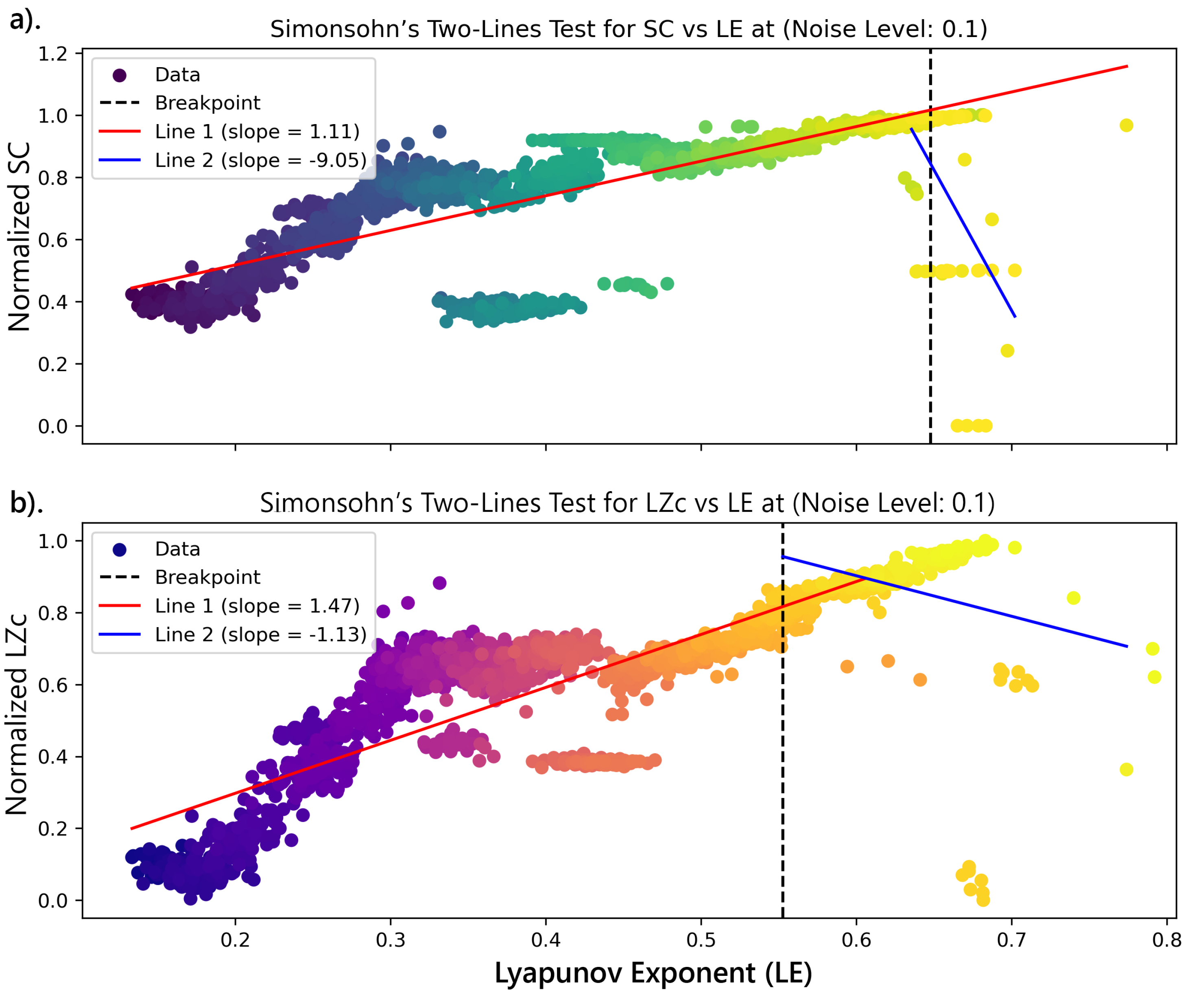
Figure 13.
Heatmaps of Complexity measures across coupling Strength and Noise Correlation in MVAR Models (a). High SC regions are observed where both coupling strength and noise correlation are either low or high, while low SC regions are found in intermediate ranges, suggesting a complex interplay between these parameters. (b) High LZc complexity found in regions with low noise correlation and moderate to high coupling strength, whereas low complexity occurs when both parameters are high. (c) and (d) illustrate the variability and distribution of SC and LZc complexities across different levels of noise correlation, highlighting the trends and the spread of complexity values within each range of noise correlation.
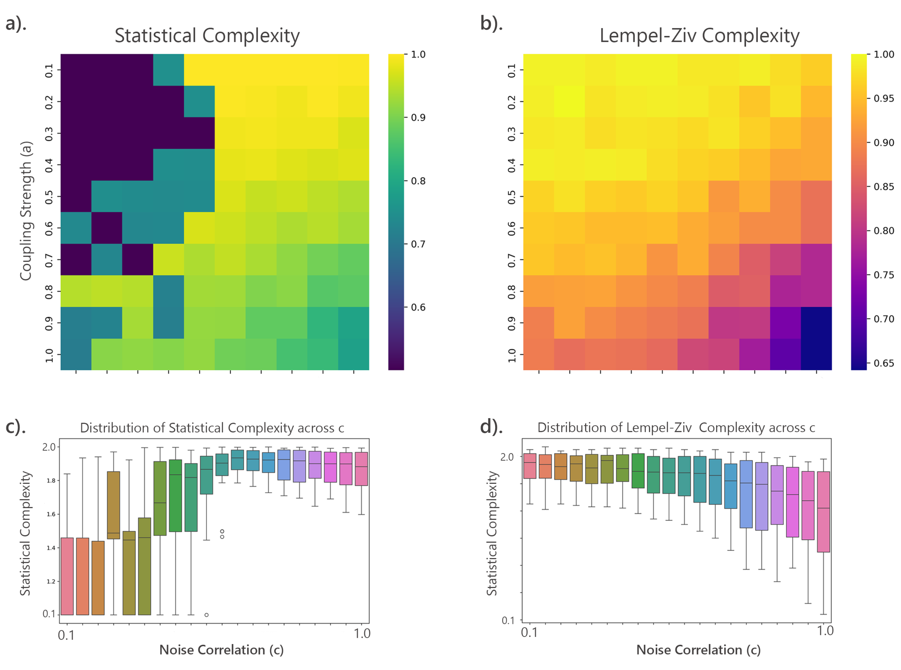
Figure 14.
The distribution of statistical complexity (SC) and Lempel-Ziv complexity (LZc) as functions of coupling strength (a) and noise correlation (c) in the MVAR model. The SC plots ((a) and (b)) highlight significant variations in complexity, with notable peaks and troughs indicating areas of high and low complexity. In contrast, the LZc complexity plots ((c) and (d)) exhibit a smoother gradient, with a general trend of decreasing complexity as noise correlation increases. The contour maps provide a detailed view of the complexity landscapes, emphasizing the system’s non-linear dynamics and sensitivity to parameter changes.
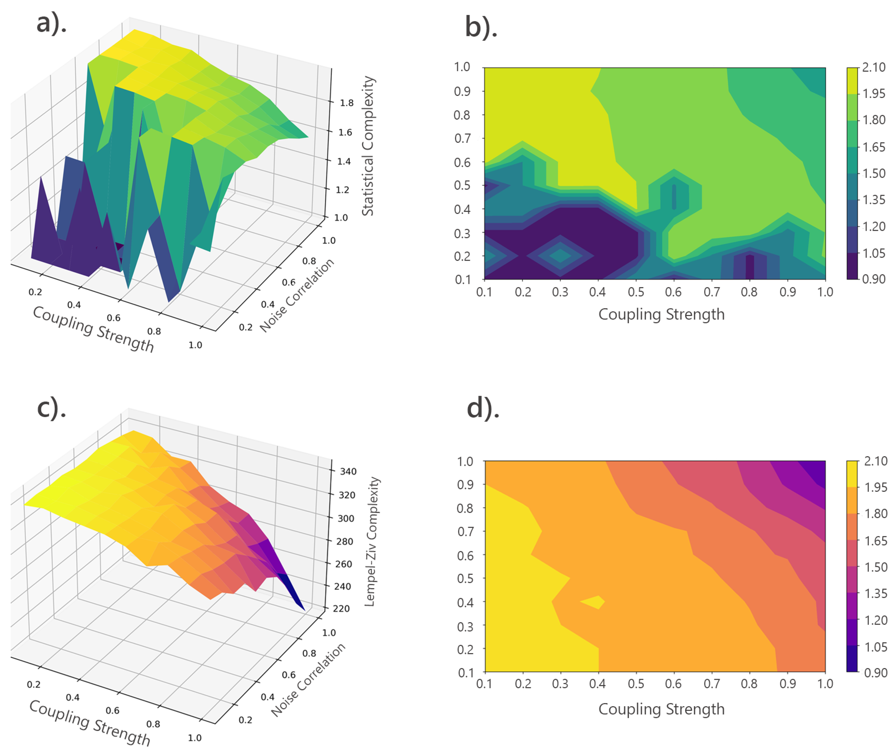
Figure 15.
Normalized values of Statistical Complexity (left panel) and Lempel-Ziv Complexity (right panel) across different states of consciousness (WR (W), REM (R), lNREM (L), eNREM (E)) for the 10 participants. The values are normalized to WR, allowing for comparison across different states. Error bars represent the standard error of the mean (SEM) calculated across all 2-second segments within each state for each participant. The results show a noticeable decrease in complexity measures during eNREM and lNREM compared to WR, while REM sleep exhibits complexity levels closer to WR.
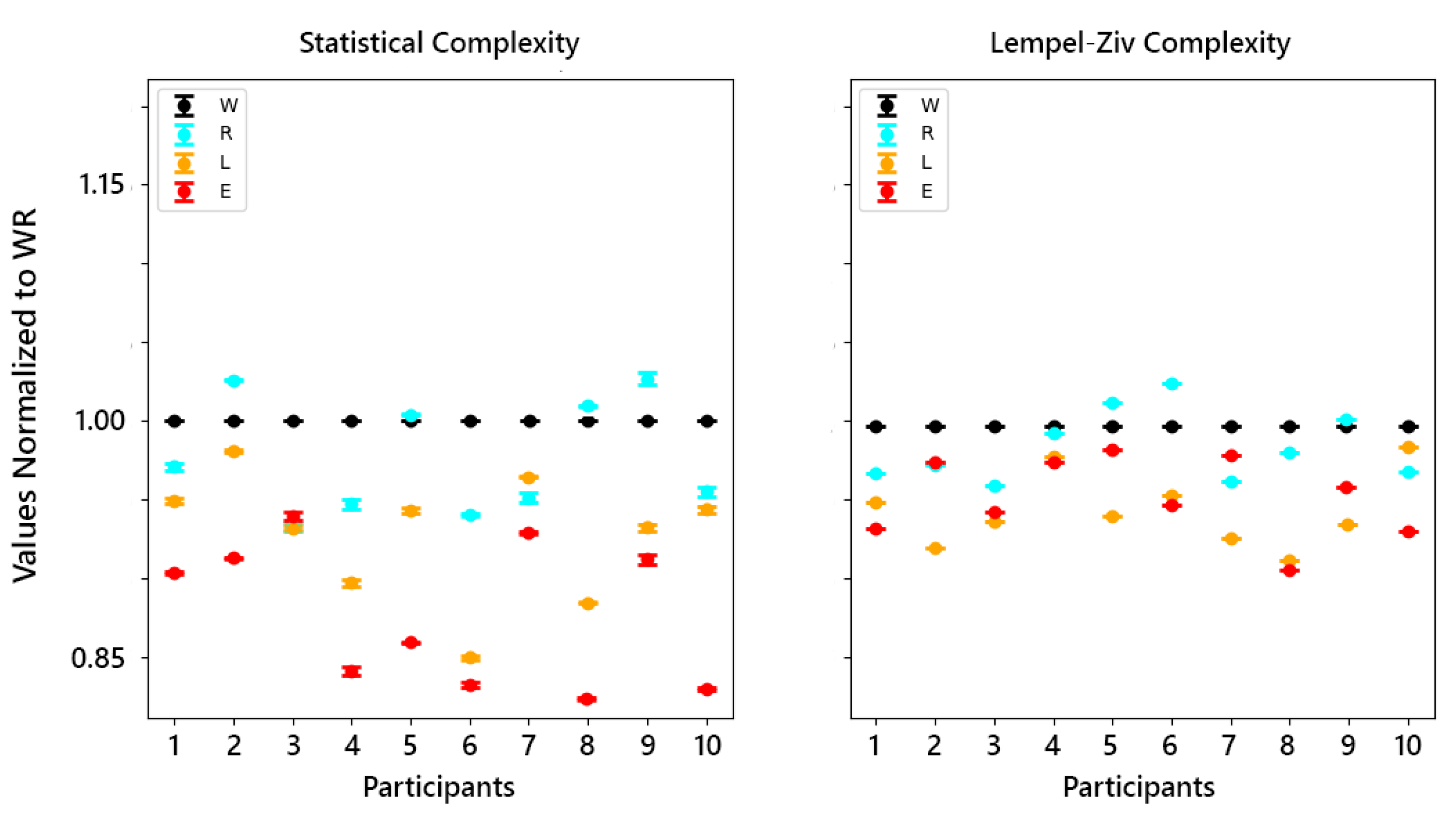
Figure 16.
Mean complexity measures with standard error across the sleep stages. a). displays the Grand Mean Statistical Complexity b).) shows the Grand Mean Lempel-Ziv Complexity for the same sleep stages. Statistical Complexity increases from eNREM to WR, with the most significant changes observed between early sleep and wakefulness. Lempel-Ziv Complexity also rises from eNREM to WR, reflecting increasing randomness and information content as the brain transitions from structured early sleep to more complex wakefulness. c). shows the heatmap of p-values from paired t-tests comparing Statistical Complexity across the sleep stages. d). displays the corresponding p-values for Lempel-Ziv Complexity. Significant differences () are indicated by darker shades, revealing clear distinctions between most stages, particularly between Early Night Sleep and other stages. Non-significant differences (), highlighted in yellow.
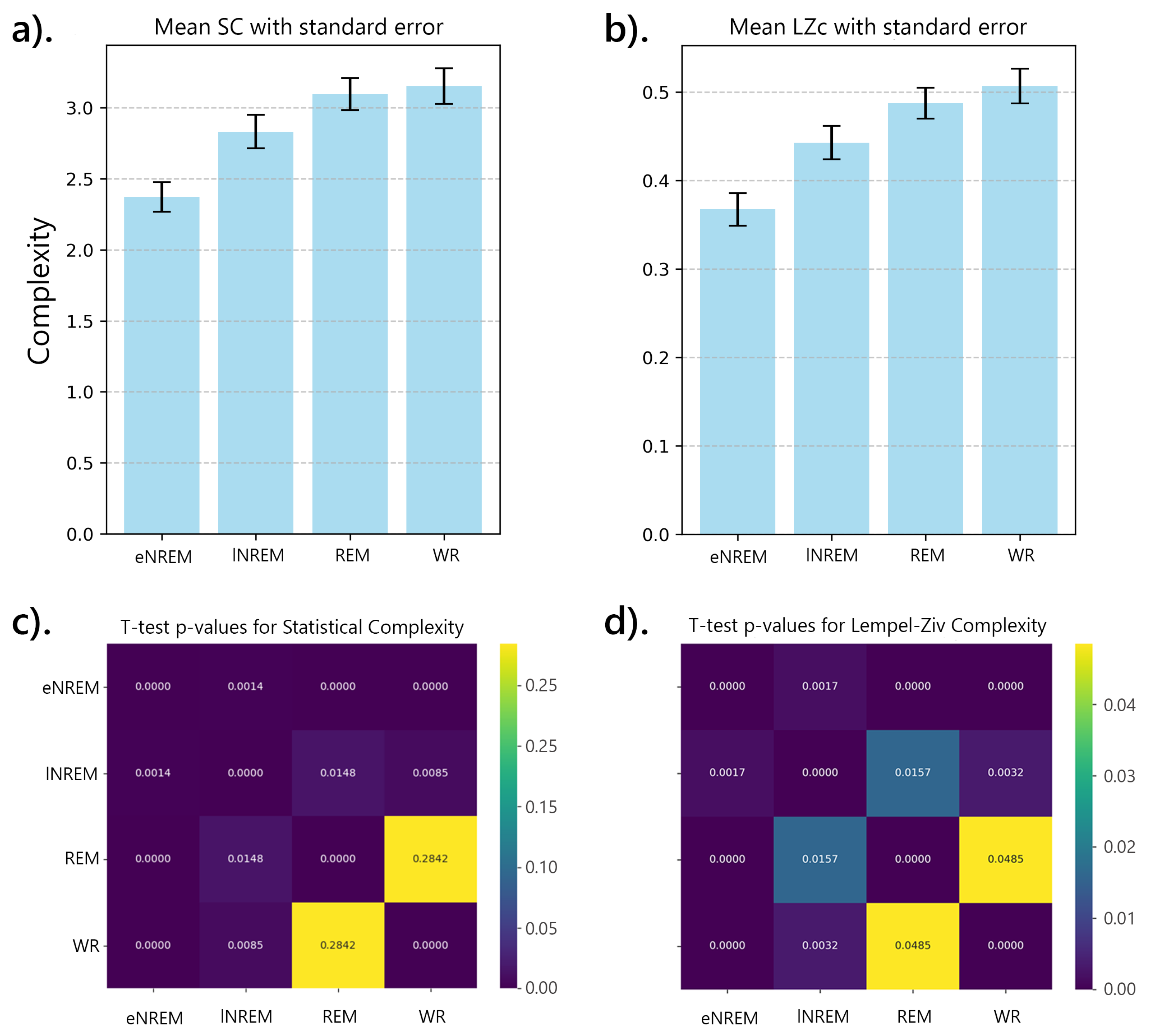
Figure 17.
Correlation Between SC and LZc Across Different Sleep States. Pearson’s correlation coefficients indicate varying relationships between SC and LZc in these states, highlighting that SC and LZc capture distinct aspects of neural complexity, with stronger correlations observed in certain states, reflecting differences in the underlying dynamics of the sleep states.
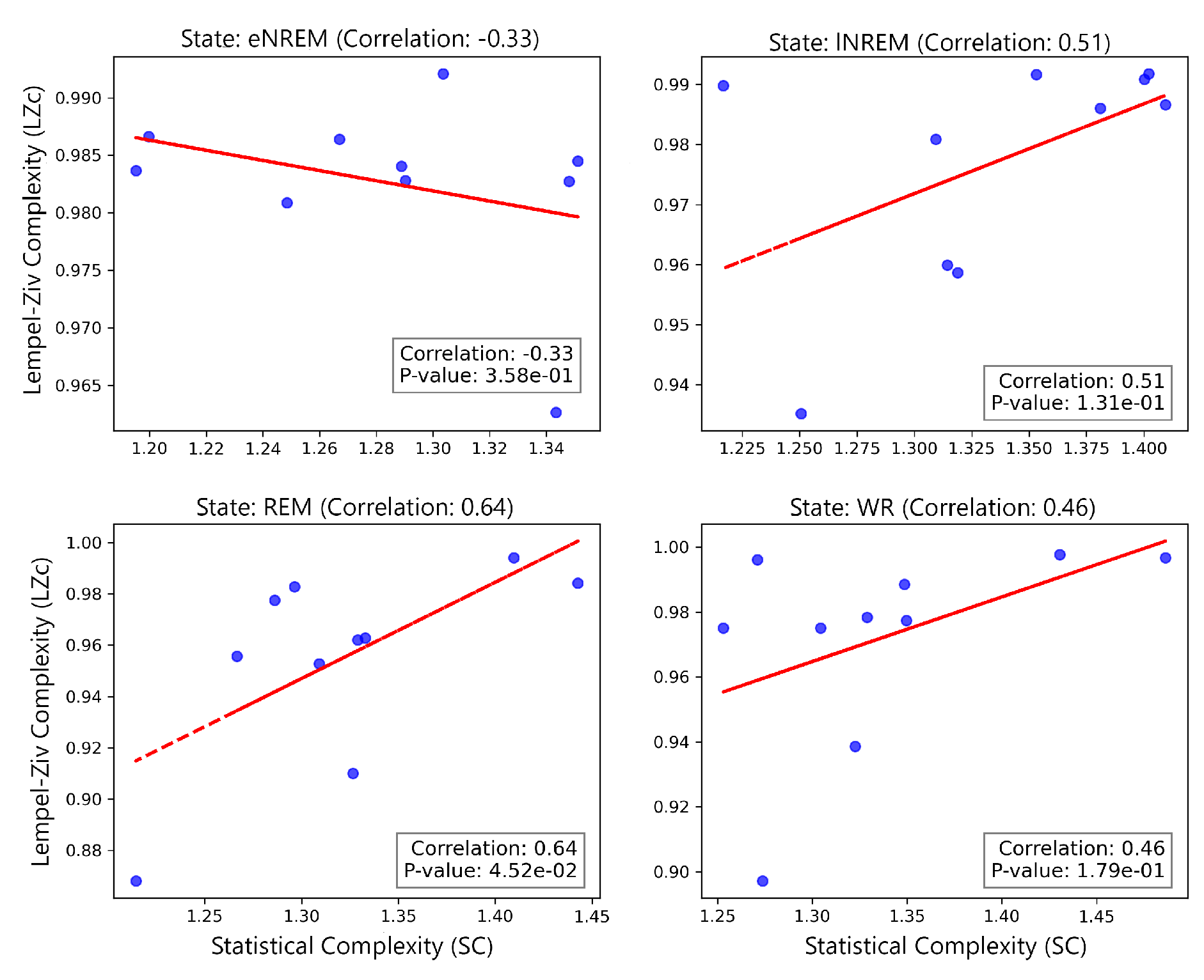
Figure 18.
Comparison of Mean Complexity Measures with Standard Error Across Sleep Stages for Statistical complexity (SC), Lempel-Ziv complexity (LZc), Approximate entropy (ApEn) and Kolmogorov complexity (KC). The error bars represent the standard error of the mean, providing a clear visual summary of how complexity measures vary across states. For all four measures, there is a general increase from eNREM state to the WR state, suggesting a trend towards higher complexity as the brain becomes more active.
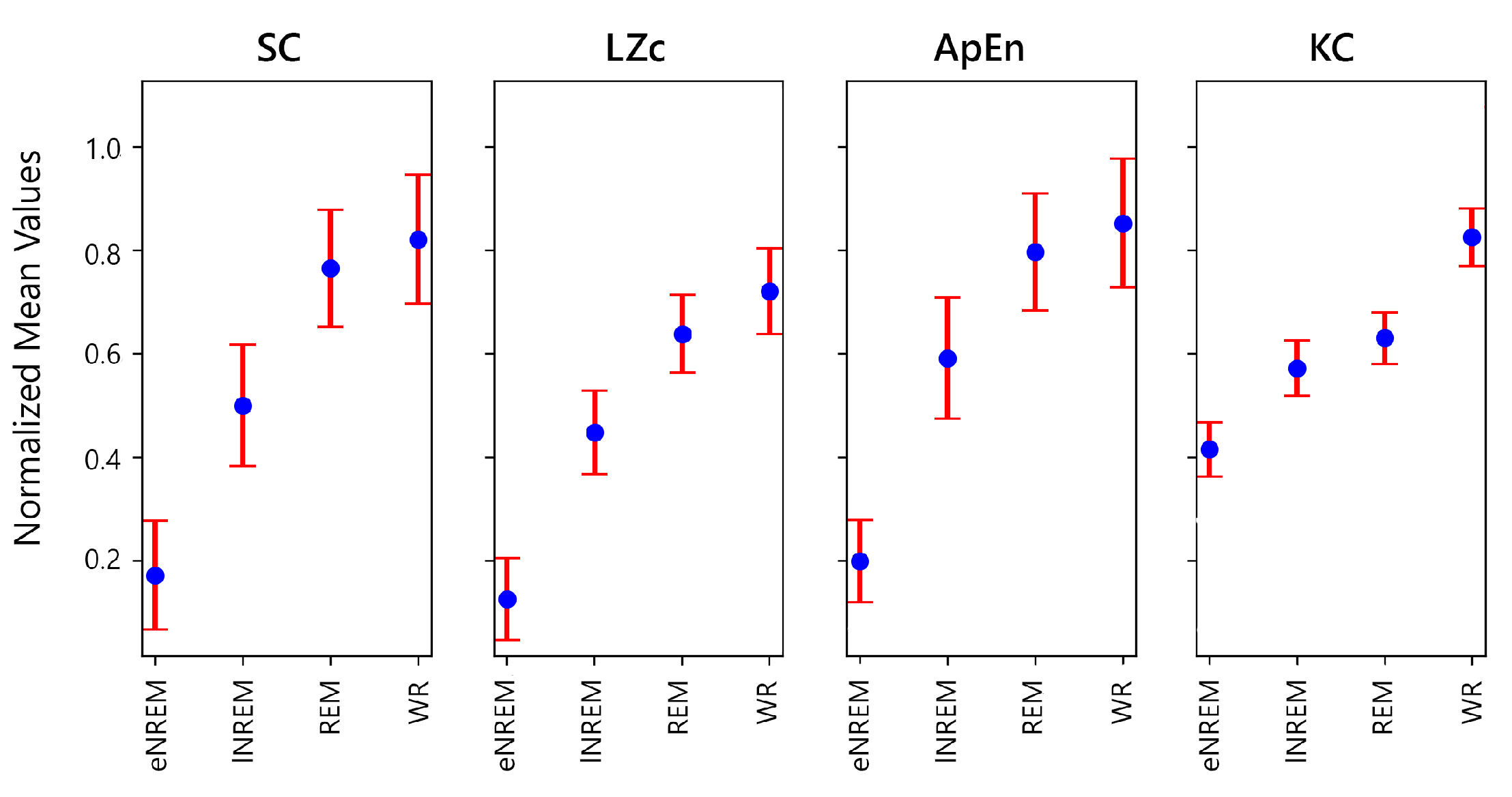
Table 1.
SC Cohen’s d results (, )
| lNREM | REM | WR | |
|---|---|---|---|
| eNREM | 1.24 | 1.99 | 2.03 |
| lNREM | 0.69 | 0.80 | |
| REM | 0.14 |
Cohen’s d results for Statistical Complexity (SC) across different sleep states. The values reflect the effect sizes of pairwise comparisons between sleep states, showing larger differences for earlier stages compared to wakeful rest (WR).
Table 2.
LZc Cohen’s d results
| lNREM | REM | WR | |
|---|---|---|---|
| eNREM | 1.21 | 2.00 | 2.20 |
| lNREM | 0.73 | 0.99 | |
| REM | 0.31 |
Cohen’s d results for Lempel-Ziv complexity (LZc), comparing different sleep states. Similar to SC, higher effect sizes are observed between earlier sleep stages and wakeful rest.
Table 3.
Results of Simonsohn’s Two-Lines Test of a U-Shaped Relationship
| Regression Line 1 | Regression Line 2 | ||
|---|---|---|---|
| SC | |||
| LZc |
Summary of the slopes (b), z-scores (z), and p-values (p) for the regression lines before and after the breakpoints identified in the analysis. The results demonstrate significant differences in the relationships between Lyapunov exponent and both Statistical Complexity (SC) and Lempel-Ziv Complexity (LZc), confirming the presence of a U-shaped pattern. High positive z-scores before the breakpoints and significant negative z-scores after the breakpoints indicate a transition from an increasing to a decreasing trend, further validating the U-shaped relationship.
Table 4.
Performance of Complexity Measures in distinguishing Sleep States
| Complexity | E vs. L | E vs. R | E vs. W | L vs. R | L vs. W | R vs. W |
|---|---|---|---|---|---|---|
| SC | Yes | Yes | Yes | Yes | Yes | Yes |
| LZc | Yes | Yes | Yes | Yes | Yes | Yes |
| KC | Yes | Yes | Yes | No | Yes | Yes |
| ApEn | Yes | Yes | Yes | Yes | Yes | No |
Comparative ability of complexity measures—SC, LZc, KC, and ApEn—to distinguish between different sleep states (early night NREM (E), late night NREM (L), REM sleep (R), and wakeful rest (W)). "Yes" indicates that the measure successfully differentiated between the states, while "No" indicates a lack of significant differentiation. The results highlight the effectiveness and limitations of each complexity measure in capturing the unique characteristics of each sleep state.
Disclaimer/Publisher’s Note: The statements, opinions and data contained in all publications are solely those of the individual author(s) and contributor(s) and not of MDPI and/or the editor(s). MDPI and/or the editor(s) disclaim responsibility for any injury to people or property resulting from any ideas, methods, instructions or products referred to in the content. |
© 2024 by the authors. Licensee MDPI, Basel, Switzerland. This article is an open access article distributed under the terms and conditions of the Creative Commons Attribution (CC BY) license (http://creativecommons.org/licenses/by/4.0/).
Copyright: This open access article is published under a Creative Commons CC BY 4.0 license, which permit the free download, distribution, and reuse, provided that the author and preprint are cited in any reuse.


