Submitted:
07 October 2024
Posted:
08 October 2024
You are already at the latest version
Abstract
A demagnetization study was conducted on a magnetically shielded room (MSR) at Fraunhofer IPM, designed for applications such as magnetoencephalography (MEG) and materials testing. With a composite of two layers of mu-metal and an intermediate aluminum layer, the MSR must provide a residual field under 5 nT for the successful operation of optically pumped magnetometers (OPM). The degaussing process, employing six individual coils, reached the necessary residual magnetic field within the central 1 m3 volume in under four minutes. Due to the low frequency shielding factor of 100, the obtained average residual field is shown to be limited by environmental residual field changes after degaussing and not by the degaussing procedure.
Keywords:
degaussing
; residual magnetic field
; magnetic shielding
; OPM
; MEG
1. Introduction
Magnetically shielded rooms (MSRs) are specialized enclosures designed to create controlled environments with reduced residual magnetic fields and minimized influence from external magnetic disturbances occurring nearby. MSRs are mainly used for bio magnetic measurements in neuroscience e.g., [1] and in fundamental physics experiments e.g., [2,3].
Research efforts have focused on achieving low residual magnetic fields and field gradients in MSRs to enable high-resolution fundamental experiments and the use of sensitive magnetic sensors [4]. Practical medical applications must satisfy additional factors like site restrictions, overall cost per measurement, preparation and measuring time, and patient’s comfort. Meanwhile, sensitive, and lightweight magnetic field detector systems have been introduced, leading to the development of wearable magnetoencephalography (MEG) systems. These advancements enable patients to move during measurements or even walk within the MSR [5,6]. Suitable magnetic field detectors for such applications are optically pumped magnetometers (OPMs). For optimal operation of OPMs an absolute magnetic field of < 5nT is required. It has been reported that such conditions can be obtained within the central 1 m3 of a 2-layer MSR [4,7].
Fraunhofer IPM in Freiburg, Germany, purchased a standard 2+1-layer MSR from VAC, Germany. The MSR consist of 2-layers mu-metal for low frequency shielding and 1 eddy current layer (aluminum) for high frequency shielding [8], thus, the nomenclature 2+1 layer MSR. The MSR walls incorporate degaussing coils. Every time the MSR is opened, the MSR and especially its door is magnetized by the external magnetic field e.g., the earth magnetic field. After closing the door, reproduceable low and stable field conditions are obtained only by degaussing the MSR [4,7,9,10]. One of the challenges is to shorten the degaussing procedure so that the MSR can be degaussed in an acceptable time after entry of a new human subject.
2. Materials and Methods
The MSR at Fraunhofer IPM is equipped with six autonomous degaussing coils, with three coils for each of the two shells. The three coils for one shell are depicted in Figure 1. Each degaussing coil consists of four individual coils positioned at the cube’s edges along one of the three MSR axes, which are connected in series to form a large toroidal coil. The z-coil generates a magnetic flux within the shielding material on a plane orthogonal to the z-axis, as shown in Figure 1. When the coil for only one axis of one shell is activated, it is referred to as an I-configuration (one color). If the coils for two axes of one shell are operated simultaneously, it is called an L-configuration (two colors). Operating the coils for all three axes of one shell simultaneously is known as a Z-configuration (all three colors).
The degaussing signal for operating the coils was generated as illustrated in Figure 1. A PC-programmed waveform generator equipped with a 16-bit analog output card from National Instruments produces the degaussing waveform, a linearly declining sinusoid that comprises 1500 periods at a frequency of 7 Hz. Prior to the amplitude decrease, the amplitude is linearly increased to its maximum over 10 periods, followed by 10 periods at the maximum amplitude to stabilize conditions. Each complete degaussing cycle takes 3 minutes and 40 seconds. Additional time is needed at the beginning, between different degaussing cycles, and at the end to disconnect, change, and connect the cables. The degaussing waveform is fed into a four-quadrant amplifier (Rohrer GmbH, Munich/Germany) to convert the voltage-driven signal into an oscillatory current-driven signal with a peak amplitude of approximately 20 A. This alternating current is then passed through a transformer to remove any residual DC offset before being applied to the selected degaussing coils within the MSR walls.
The MSR was demagnetized by applying degaussing fields in multiple configurations, followed by mapping the residual field in a central 1 m³ volume using a 3-axis Bartington fluxgate (MAG03 MCL 70). Measurements were taken on a 25 cm grid at 125 positions (5 x 5 x 5). Figure 2 shows the equipment used for degaussing the MSR and mapping the field. The field scan was manually performed by a non-magnetic person inside the MSR and was completed within 26 minutes. To minimize systematic uncertainty in the static residual field measurement the offset was measured before and after a full scan, which took an additional 3 minutes. Alongside the fluxgate inside the MSR, readings from an exterior reference fluxgate (MAG03 MC 1000) were also recorded.
Initially, we conducted an inspection of the residual field in the MSR using a small, single-channel fluxgate mounted on a wooden rod, which was inserted into the MSR through a feedthrough hole. Our objective was to verify that the sequential degaussing procedure for the x-, y-, and z-degaussing coils on both the outer and inner layers effectively reduces the residual field. This method was first reported in [4]. Subsequently, three configurations for fast degaussing were tested with a person inside the MSR who scanned the field distribution post-degaussing. The three configurations are as follows:
- posI: Interconnecting the I-configuration of both shells in series, instead of operating them individually, which halves the degaussing time. The coils were connected such that the magnetic fields in the inner and outer shells point in the same direction.
- negI: Replicating the first configuration but reversing the polarity. While this does not reduce the degaussing time compared to the posI configuration, it helps evaluate the reproducibility and imperfections of the degaussing function.
- posZ: Interconnecting all coils—across both shells and in all three directions—in series. This allows for the complete degaussing of the MSR in a single operation. The degaussing time is reduced by another factor of three, making it six times faster than a single coil configuration and eliminating the need for additional time to change the connections of the different degaussing coils. Note that „posZ” indicates the connection of the three I-coils, not the geometric axis.
During the measurement campaign, the shielding factor (SF) of the MSR was measured along three spatial directions to aid in interpreting the residual field maps. A set of three Helmholtz-like coil systems, permanently installed outside the MSR, were used to apply the excitation field. The same apparatus as shown in Figure 1 was used to drive the coils, except for the transformer. Additionally, an automated switch controlled by the PC was incorporated to toggle between the Helmholtz coils in different directions. This setup enabled automated data acquisition at night, which is crucial as low-frequency measurements require extended measurement times.
3. Results
The measured shielding factor curve (Figure 3) is typical for this type of MSR.
The low-frequency shielding factor for (f → 0), known as the quasi-static shielding factor, is approximately 100 in all three MSR directions. Considering ongoing discussions about the specifications of the measurement conditions, we also examined the dependence of SF at 0.02 Hz on the applied excitation amplitude, as shown in Figure 3. Within the measured amplitude range, the SF increases almost linearly, with a slight reduction in slope at larger amplitudes. This dependence is significant enough that the measurement conditions should be clearly specified when purchasing an MSR and when calculating expected damping factors from SF curves or values provided by the manufacturer.
During field mapping, we consistently observed approximately 125 nT changes in the external field. The expected change in the internal field is about 1/100 of this external fluctuation, which amounts to up to 1.25 nT. This expectation was confirmed by repeated measurements at the central point of the MSR, taken before and after completing a z-layer with 25 points, followed by moving the fluxgate to the next z-layer. The external field changes exhibited stable sections around an average value, interrupted by brief periods of rapid variations around this average. A clear correlation was identified between the time trace of the external field and the field inside the MSR at the central point. This relationship can be mathematically described by a proportional constant and a linear component, using the formula:
The constant c represents the attenuation of the external field by the MSR and is dependent on SF and the position of the reference fluxgate. The line accounts for the DC-offset drift of the measuring equipment and low-frequency drift of the environmental field. The DC offset of the internal fluxgate was determined inside the MSR before and after a field scan, with differences consistently below 0.4 nT. A correction was applied to the data to account for external field changes during mapping, using the average external field during the scan as a reference and performing the linear correction with respect to the midpoint of the scan time. The constants a, b, and c were optimized using a least-squares fit with the Microsoft Excel add-in solver.
It was found that there were no significant differences in the field maps whether the optimization was done separately for each measurement or through an overall fit with the same constant c for all measurements, as the reference fluxgate position was not changed between measurements. The corrected field maps were smoother because most inconsistencies observed in the original sequentially measured data were successfully removed. As a result, we only present the corrected 3D field maps.
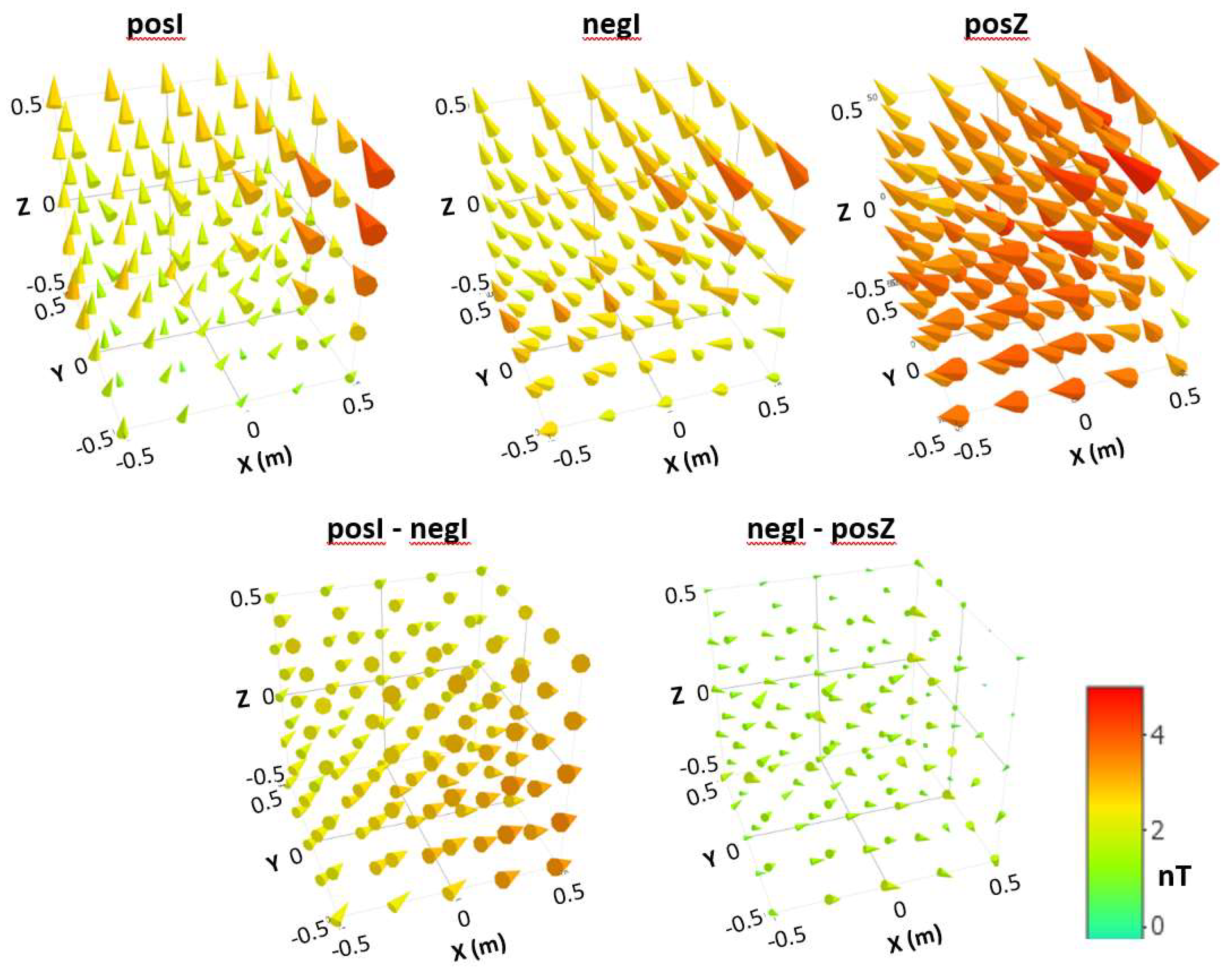
All field values are below 5 nT within the 1 m³ central volume, even without corrections for external disturbances and apparatus DC-offset drifts. There is no significant change in the residual field direction. A significant change would suggest insufficient cycles or an excessively high amplitude difference in the degaussing function when comparing posI and negI. This indicates that the number of periods in the degaussing function is adequate. The 3D maps are generally uniform, except for a few points near the front door. This non-uniformity was traced to overly magnetic screws in the MSR door assembly. Calculating the difference between two field maps cancels out most of the fields around the door. What remains is a homogeneous field that increases in the average direction of the residual field towards the door for the posI-negI difference. In contrast, the difference between negI and posZ is nearly random.
Figure 4.
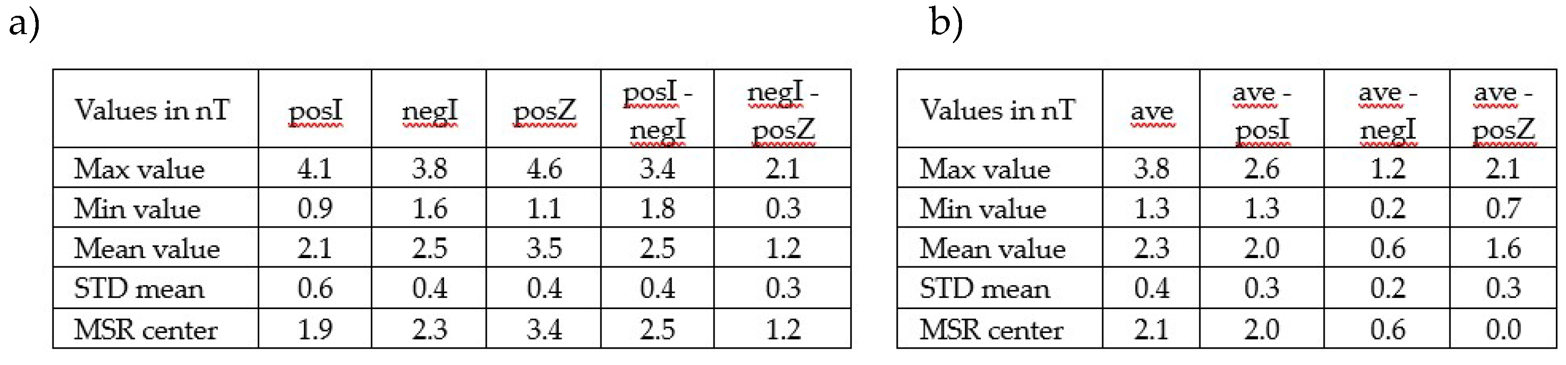
Illustration of the measured 3D field distributions for the three different degaussing configurations: posI, negI, and posZ (top row). Below, the difference between the respective 3D maps is shown. All maps use the same color code. Table 1a provides characteristic values for these 3D field illustrations. Note that the scaling of the height of the cones relative to the absolute field value reveals minor differences in the maximum amplitude, attributed to a much larger base surface. The difference between negI and posZ is minimal because both fields have a similar direction, whereas posI and negI exhibit slightly different directions.
Figure 4.
Illustration of the measured 3D field distributions for the three different degaussing configurations: posI, negI, and posZ (top row). Below, the difference between the respective 3D maps is shown. All maps use the same color code. Table 1a provides characteristic values for these 3D field illustrations. Note that the scaling of the height of the cones relative to the absolute field value reveals minor differences in the maximum amplitude, attributed to a much larger base surface. The difference between negI and posZ is minimal because both fields have a similar direction, whereas posI and negI exhibit slightly different directions.

4. Discussion
Using the posZ configuration, where all six degaussing coils are connected in series, the residual field within the central cubic meter of the MSR can be reduced to less than 5 nT with just one degaussing sequence lasting only 3 minutes and 40 seconds. By employing PC-operated switches, as shown in Figure 1, to manage the connection and disconnection of the degaussing coils, the entire demagnetization process can be completed in less than 4 minutes after closing the MSR door. This approach is more than six times faster than the traditional sequential degaussing of individual coils. Unlike the method presented in [7], our study demonstrates an approach using a Z configuration that completes the degaussing process in under four minutes.
Even without further optimization, this timing is sufficiently brief for conducting sequential human subject measurements. It is anticipated that decreasing the number of degaussing cycles and using a degaussing function that decreases faster than linearly could further reduce the total degaussing time. This would enable larger amplitude steps to reveal significant differences between posI and negI measurements earlier. Although magnetic field variations in the MSR environment during mapping were successfully corrected, there remains some uncertainty about potential variations in the average environmental magnetic field between the mapping and degaussing phases.
The maximum field values observed during all three degaussing processes were primarily attributed to magnetic screws located in the MSR door, particularly one near the top-right corner. To enhance the homogeneity and average field within the central volume, these A4 type stainless steel screws were afterwards replaced with titanium screws.
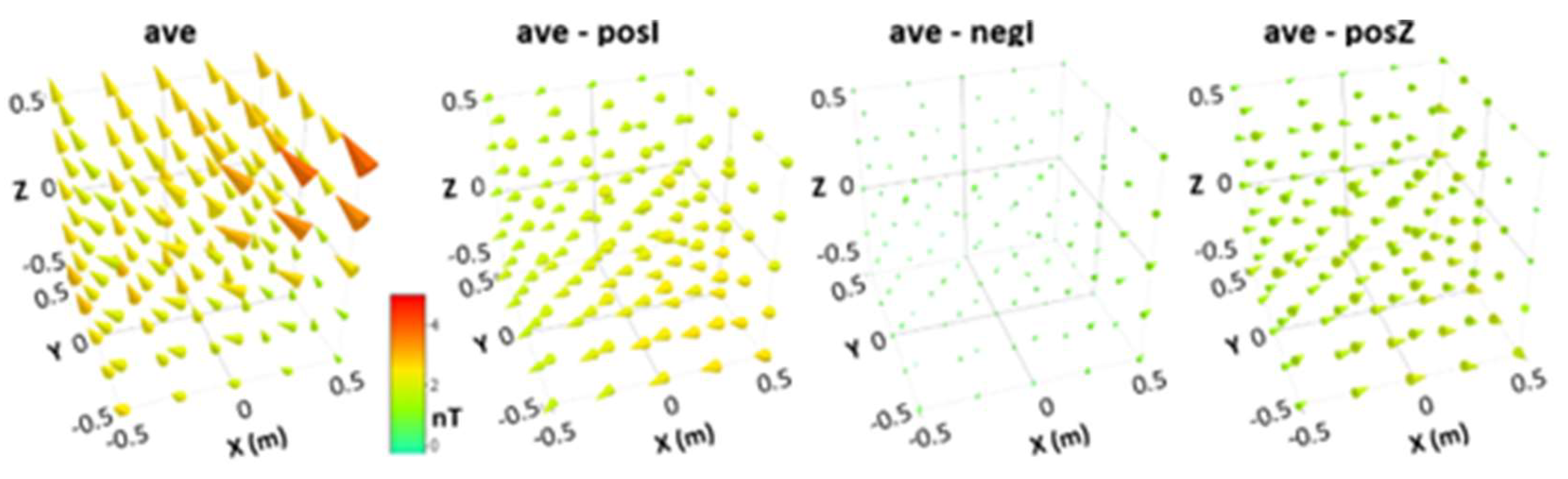
The influence of the screws can be almost completely neutralized mathematically by calculating an average 3D field from the measured maps and then determining the differences between this average and the three individual measurements. These calculations help visualize the variations between the measured maps.
The difference relative to the negI 3D map appears nearly random, suggesting it closely aligns with the average 3D map. In contrast, the differences between both posI and posZ relative to the average are significantly larger and in opposite directions, which is expected since the negI field closely matches the overall average.
All three differential 3D maps display a homogeneous field that increases in amplitude toward the door, albeit barely noticeable for negI. This pattern strongly suggests that the observed differences in the residual field are predominantly influenced by changes in the external magnetic field between the degaussing and field mapping phases. However, it may also be impacted by the external field during the degaussing process, which was not recorded.
Degaussing aims to equilibrate the MSR’s magnetic environment with the external field. The observed residual field after degaussing at the MSR’s center (see Table 1a) is below 3.5 nT, which is by a factor of 11,700 lower than the surrounding environmental field. Therefore, a hypothetical environmental field difference of 1 µT during different degaussing attempts would result in a center field difference of less than 90 pT, which is beyond the resolution of the fluxgate. This effectively rules out the influence of the surrounding field during degaussing as the cause of the differences shown in Figure 5.
The different maps in Figure 5 were analyzed for magnetic field contributions resembling a curl, with a center near the MSR’s core, regardless of the chosen viewpoint. After accounting for distortions caused by the overly magnetic screws, no such curl patterns were detected down to the resolution limit of the field maps. Typically, a curly static field contribution might be expected if there is a discrepancy in the DC current offset between two degaussing cycles, or if there is an excessively large change in current steps between cycles when the number of degaussing cycles is insufficient.
By ruling out variations in the environmental field during degaussing and differences in the degaussing procedure as causes for the observed discrepancies in Figure 5, the remaining plausible explanation is a change in the magnetic field surrounding the MSR post-degaussing only damped by the low frequency SF of about 100. The computed 3D field maps support this hypothesis, indicating that the amplitude of the homogeneous internal field correlates with the difference between the average field during the scan and the average field derived from the individual scans’ average fields. For the negI map, the difference is so small that the resolution of the fluxgate and the mechanical precision of its position and axis orientation adjustment become the limiting factors.
To enhance field stability for scans and subsequent practical applications, installing an active field compensation system could be beneficial. This system would stabilize the magnetic field around the MSR immediately after degaussing. Additionally, it could maintain field stability during degaussing if the bandwidth of the compensation system is restricted to well below the degaussing frequency of 7 Hz using a low-pass filter incorporated into the feedback loop.
5. Conclusions
The two-layer VAC-MSR at Fraunhofer IPM in Freiburg, Germany, which features a low-frequency shielding factor of 100, underwent degaussing processes using different coil configurations that achieved a short degaussing time. This procedure demonstrated that less than four minutes are sufficient to degauss the shield after it has been opened and subsequently closed for the next measurement. This process successfully achieved a residual magnetic field of less than 5 nT in the central 1 m³ and maintained stable field conditions suitable for the operation of OPMs.
The limitation for the field inside the MSR is not governed by the environmental magnetic field during the degaussing process but rather by changes in the environmental field at the MSR location post-degaussing, which are only attenuated by a shielding factor of 100. Future enhancements will involve the use of active shielding by utilizing the SF-test coils permanently installed on the MSR to further dampen the observed magnetic field changes at the MSR site.
To achieve significantly lower residual fields, it is crucial to avoid using even slightly magnetic materials inside the shield. Implementing a more robust overall shielding strategy is fundamental. This can be accomplished through active shielding and the removal of overly magnetic components. With these improvements, it is anticipated that a reproducible residual field of below 1 nT in the central cubic meter can be attained. This goal will ultimately depend on the coil configurations and the degaussing function of the MSR.
Author Contributions
All authors participated in the measurements presented in this paper. Peter Koss and Allard Schnabel prepared the initial draft, which was subsequently reviewed and improved by all authors.
Funding
This work was supported by the Fraunhofer project MSR-QUANTUM.
Institutional Review Board Statement
Not applicable.
Informed Consent Statement
Not applicable.
Data Availability Statement
The data is available from the authors upon reasonable request.
Conflicts of Interest
The authors declare no conflicts of interest.
References
- Waterstraat, Gunnar and Körber, Rainer and Storm, Jan-Hendrik and Curio, Gabriel, “Noninvasive neuromagnetic single-trial analysis of human neocortical population spikes,” Proceedings of the National Academy of Sciences, no. 118, 2021.
- N. J. Ayres et al., “The very large n2EDM magnetically shielded room with an exceptional performance for fundamental physics measurements,” The Review of scientific instruments, vol. 93, no. 9, p. 95105, 2022. [CrossRef]
- N. J. Ayres et al., “Achieving ultra-low and -uniform residual magnetic fields in a very large magnetically shielded room for fundamental physics experiments,” The European physical journal. C, Particles and fields, early access. [CrossRef]
- Jens Voigt, Silvia Knappe-Grüneberg, Allard Schnabel, Rainer Körber, and Martin Burghoff, “Measures to reduce the residual field and field gradient inside a magnetically shielded room by a factor of more than 10,” Metrology and Measurement Systems, 2013, Art. no. 20.
- N. Holmes et al., “A lightweight magnetically shielded room with active shielding,” Scientific reports, early access. [CrossRef]
- N. Holmes et al., “Enabling ambulatory movement in wearable magnetoencephalography with matrix coil active magnetic shielding,” NeuroImage, early access. [CrossRef]
- I. Altarev et al., “Minimizing magnetic fields for precision experiments,” Journal of Applied Physics, vol. 117, no. 23, 2015, Art. no. 233903. [CrossRef]
- K. Yamazaki, K. Muramatsu, M. Hirayama, A. Haga, and F. Torita, “Optimal Structure of Magnetic and Conductive Layers of a Magnetically Shielded Room,” IEEE Trans. Magn., vol. 42, no. 10, pp. 3524–3526, 2006. [CrossRef]
- Z. Sun et al., “Limits of Low Magnetic Field Environments in Magnetic Shields,” IEEE Trans. Ind. Electron., vol. 68, no. 6, pp. 5385–5395, 2021. [CrossRef]
- J. Yang et al., “Demagnetization Parameters Evaluation of Magnetic Shields Based on Anhysteretic Magnetization Curve,” Materials (Basel, Switzerland), early access. [CrossRef]
Figure 1.
Schematic illustration of the experiment’s layout established to degauss the MSR. The identically colored coils on the edges are interconnected in series so that the magnetic field induces a complete magnetic loop inside the shielding material around the inner volume, as indicated by the blue arrows for the blue coils.
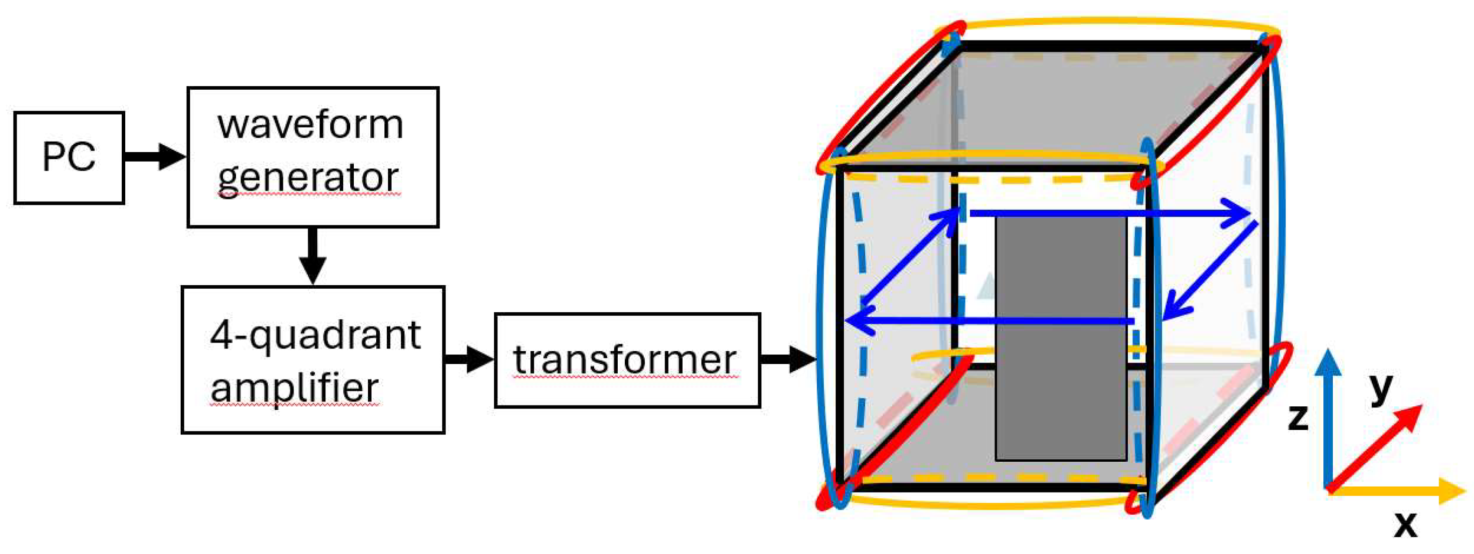
Figure 2.
Images of the experimental setup elements. On the left: a picture of the mapping framework using an aluminum rail to adjust the x-y position of the pole, allowing the fluxgate to be positioned at different z-positions. On the right: a photo of the four-quadrant amplifier (black) that drives the degaussing current through the degaussing coil and the transformer (large white box) to eliminate DC offsets.
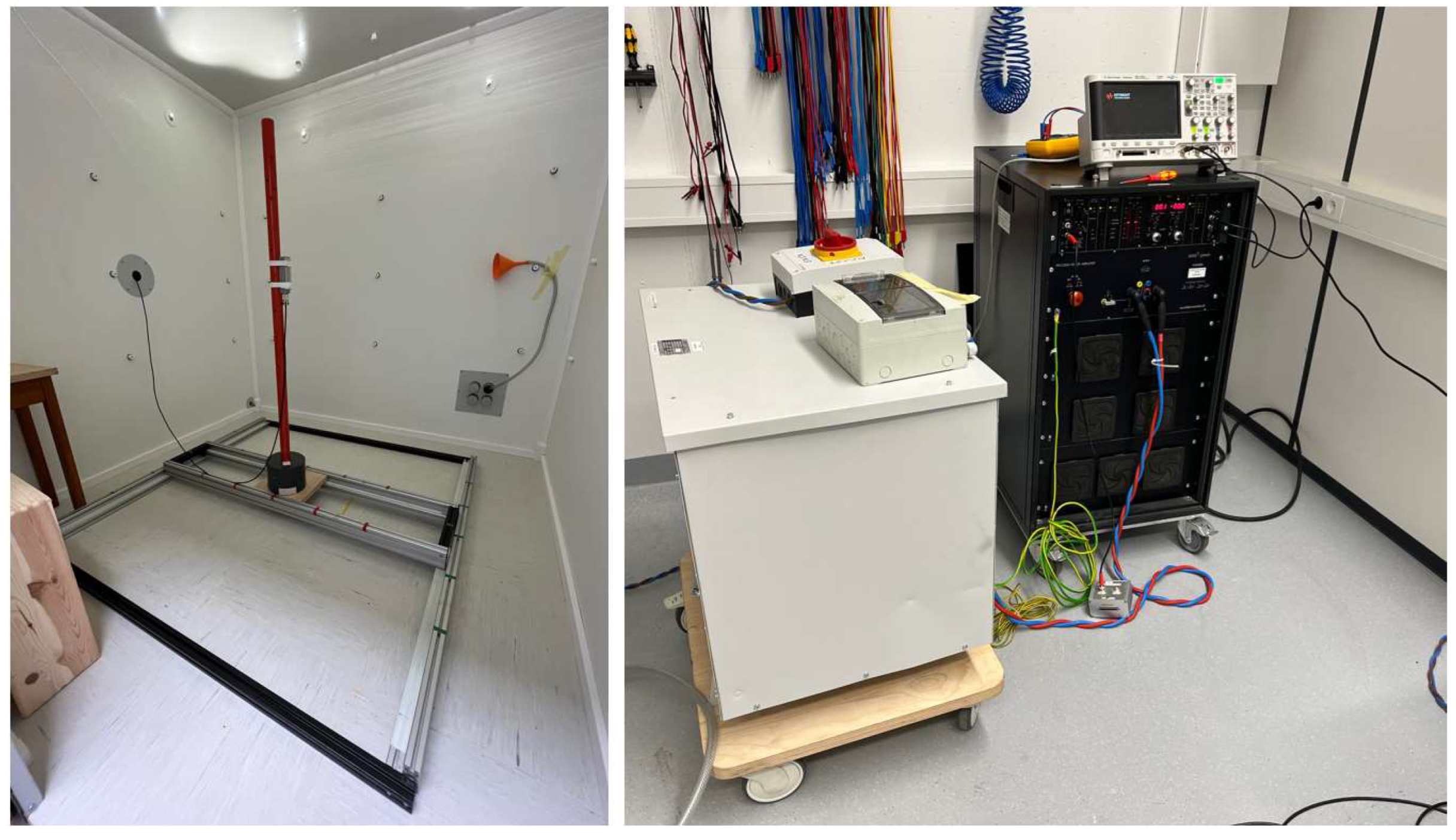
Figure 3.
Measured shielding factor (SF) curves for the three axes of the two-layer MSR with a 1µT effective excitation field strength. In the inset: Dependence of SF at 0.02 Hz on the amplitude of the excitation field.
Figure 3.
Measured shielding factor (SF) curves for the three axes of the two-layer MSR with a 1µT effective excitation field strength. In the inset: Dependence of SF at 0.02 Hz on the amplitude of the excitation field.
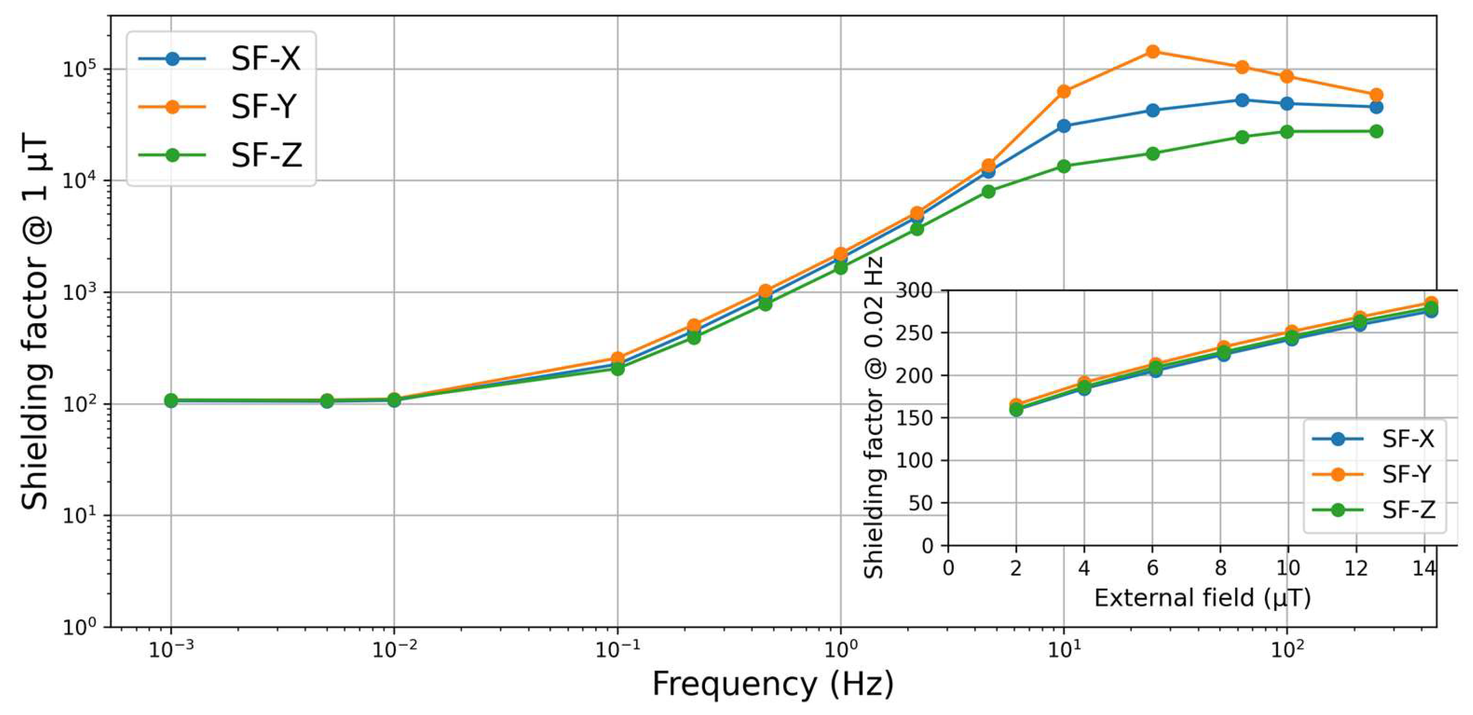
Figure 5.
Average field map (ave) and the differences between it and the maps of posI, negI, and posZ. All maps share the same color code. Table 1b provides characteristic values for these 3D field maps.
Figure 5.
Average field map (ave) and the differences between it and the maps of posI, negI, and posZ. All maps share the same color code. Table 1b provides characteristic values for these 3D field maps.
Disclaimer/Publisher’s Note: The statements, opinions and data contained in all publications are solely those of the individual author(s) and contributor(s) and not of MDPI and/or the editor(s). MDPI and/or the editor(s) disclaim responsibility for any injury to people or property resulting from any ideas, methods, instructions or products referred to in the content. |
© 2024 by the authors. Licensee MDPI, Basel, Switzerland. This article is an open access article distributed under the terms and conditions of the Creative Commons Attribution (CC BY) license (http://creativecommons.org/licenses/by/4.0/).
Copyright: This open access article is published under a Creative Commons CC BY 4.0 license, which permit the free download, distribution, and reuse, provided that the author and preprint are cited in any reuse.


