Submitted:
04 October 2024
Posted:
08 October 2024
You are already at the latest version
Abstract
Credit scoring is a cornerstone of financial risk management, enabling financial institutions to assess the likelihood of loan default. However, widely recognized contemporary credit risk metrics, like FICO or Vantage scores, remain proprietary and inaccessible to the public. This study aims to devise an alternative credit scoring metric that mirrors the FICO score, using an extensive dataset from Lending Club. The challenge lies in the limited insights available on both the precise analytical formula and the comprehensive suite of credit-specific attributes integral to the FICO score's calculation. Our proposed metric leverages basic information provided by potential borrowers, eliminating the need for extensive historical credit data. We aim to articulate this credit risk metric in a closed analytical form with variable complexity. To achieve this, we employ a symbolic regression method anchored in Genetic Programming (GP). Here, Occam's razor principle guides evolutionary bias towards simpler, more interpretable models. To ascertain our method's efficacy, we juxtapose the approximation capabilities of GP-based symbolic regression with established machine learning regression models, such as Gaussian Support Vector Machines (GSVMs), Multi-Layer Perceptrons (MLPs), Regression Trees and Radial Basis Function Networks (RBFNs). Our experiments indicate that GP-based symbolic regression offers comparable accuracy with these benchmark methodologies. Moreover, the resultant analytical model offers invaluable insights into credit risk evaluation mechanisms, enabling stakeholders to make informed credit risk assessments. This study contributes to the growing demand for transparent machine learning models by demonstrating the value of interpretable, data-driven credit scoring models.
Keywords:
Credit Risk Assessment
; Neural Networks
; Support Vector Machines
; Genetic Programming
; Radial Basis Functions Networks
1. Introduction
Credit scoring comprises a vital component of financial risk management that lays the foundations for estimating the probability that a given individual will be incapable of repaying his/her dept obligations, i.e., the probability of default for a future loan [1]. Acquiring an accurate measure for the probability of default allows banking agencies to verify certain aspects of a particular credit product such as the loan amount, the repayment method and the interest rate [2]. In this context, optimizing lenders’ decisions on whether to offer or deny credit relies on the ability to design such credit rating measures [3] that will be able to quantify the financial condition and the creditworthiness of a candidate borrower [4]. The most prominent and widely used credit score in the banking industry is the FICO score, a measure developed in 1989 by the Fair, Isaac and Company (FICO), a company operating on the sector of data analytics focusing on credit scoring services [5]. During the past decades FICO has evolved to become the standard credit risk measure utilized by financial institutions in the United States (U.S.), facilitating decisions on whether to lend money or issue credit. Later, in 2006, the top three credit bureaus in the U.S., i.e., Equifax, TransUnion, and Experian collaborated to create the Vantage Score credit rating as an alternative to the FICO score[6].
FICO score is represented as a three-digit number, ranging from 300 to 850. The higher the score, the better the credit profile of a borrower, as higher scores are indicative of a lower default risk. Credit scores from 580 to 669 are considered “fair”, while scores from 670 to 739 are considered “good”. The key factor for deriving a credit score is the credit history, e.g. total debt, repayment history, etc. The FICO scoring methodology is based on both positive and negative credit data contained in an individual’s credit report. In particular, five main categories are considered: credit payment history, current debt level, types of credit used, length of credit history and new credit [7]. The aforementioned factors are included in credit score calculations, but they are not given equal weighting. Although, the weighting schemes of these factors are known, the exact computational methodology for determining the FICO score remains a black box. In the same vein, the algorithmic process underpinning the risk evaluation related with the Vantage Score is obscured. It is, nonetheless, noted that supplementary machine learning techniques are indeed employed in the risk assessment process, especially, when dealing with consumers whose credit data are extremely sparse [8].
Credit scoring models are, in general, not publicly available even though the U.S. legislation mandates that at least four primary factors affecting their credit score should be available to consumers. In addition, U.S. law, such as the Consumer Credit Protection Act (CCPA), provides consumer protections against lenders. In compliance with CCPA, the use of personal information is prohibited on calculating credit scores. Specifically, information about the race, color, religion, national origin, sex, marital status and age among others cannot be employed [9,10].
Bearing in mind the inherently vague nature of the credit risk assessment process, it is easy to deduce that quantifying the probability of default is an extremely difficult task. In fact, the complexity of the underlying problem is significantly increased when considering the additional restrictions on the utilization of a candidate borrower’s personal data which are imposed by the relevant legislation. In this study, we aim at developing an alternative credit scoring mechanism that will mimic the behavior of the original FICO score in a large collection of loan data operating, however, on a limited amount of consumer-specific credit information. For this purpose, we employ a substantial database of loan-related data gathered from Lending Club, a renowned peer-to-peer lending platform in the U.S. [11]. Peer-to-peer (P2P) lending companies mostly offer their services online, forming online financial communities that connect borrowers with investors (lenders). Although Lending Club became the world’s largest peer-to-peer lending platform, at the end of 2020 was announced that will no longer operate as a peer-to-peer lender as the Lending Club acquired Radius Bank and the focus switched to institutional investors.
The peer-to-peer lending platforms provide the investors with the information supplied by the borrowers when apply for a loan. Lending Club offers further details about the creditworthiness of the borrower, the type of the loan as well as a loan credit grade. A credit grade is assigned to each loan, which determines the payable interest rate and the loan processing fees. A survey for studies devoted to peer-to-peer lending can be found in [12]. A data-driven model for the estimation of P2P loans’ expected return and risk is developed in [13] by employing data obtained from Prosper P2P lending platform [14].
Credit scoring models based on machine learning methods lowers expected credit losses, according to [15], as a comparison of Logistic Regression, Multivariate Adaptive Regression Splines (MARS), SVM, Random Forest, Extreme Gradient Boosting (XGBoost) and Neural Network models trained on non-synthetic data from a Survey of Consumer Finances achieved better performance compared to FICO credit scoring in 2001s. Also, a Bayesian network model is employed in [16] for the credit risk scoring in consumer lending based on data of a firm that provides credit and loans in Singapore. Linear Regression is also used in [17] for credit scoring where it has similar performance with a SVM model, it outperforms a decision tree classifier, but it under-performs two ensemble methods (random forest and stacking with cross-validation). A dynamic ensemble classification based on soft probability was proposed in [18]. Because ensemble methods lack interpretability, the Logistic Regression remains the benchmark in the credit risk industry, so in [19,20] a high-performance and interpretable credit scoring method called penalised logistic tree regression (PLTR) is introduced, which uses information from decision trees to improve the performance of Logistic Regression.
Several approaches for credit risk scoring have been developed based on the data obtained from Lending Club. The P2P credit grading is modelled as a cost-sensitive multi-class classification problem in [21]. The performance of the Logistic Regression model, Neural Networks and ensemble models was investigated in [22]. In [23], SHAP is used in order to explain the output of a Linear Regression model and compute the feature important weights to compare them to counterfactual explanations. A comparison of Linear Regression, Random Forest and Multilayer Perceptron models for a class imbalance problem is done in [24] where the approaches are evaluated in terms of their explainability by eXplainable Artificial Intelligence (XAI) tools. An innovative credit risk prediction framework that fuses base classifiers based on a Choquet fuzzy integral improves creditworthiness evaluations in [25]. On the other hand, profit scoring approaches are proposed in [26,27] instead of determining the probability of default for a future loan.
Efforts have been made in order to use GP for credit risk scoring. In [28], a multi-gene genetic programming approach to symbolic regression did not yield a better predictive ability than Logit Transformed Regression, Beta Regression and Regression Tree for estimating the credit risk parameter LGD. GP proved by [29] to provide better results than generic credit scoring models in both classification accuracy and profit, while achieving similar classification accuracy compared with Logistic Regression, SVM, and Boosted Trees. Similar results have been achieved in [30], as GP outperformed Classification and Regression Tree (CART) and Rough Sets, but had similar results with NN and Logistic Regression. In [31], two-stage genetic programming (2SGP) incorporates the advantages of the IF-THEN rules and the discrimination function and manages to outperform GP, MLP, CART, C4.5, Rough Sets and Logistic Regression. A novel hybrid model which uses evolutionary computation, ensemble learning and deep learning was proposed in [32] and achieved high prediction accuracy for bank credit evaluation.
In this paper, we develop an alternative credit scoring mechanism that approximates the risk evaluation pattern exhibited by FICO in a large-scale collection of loan data. In particular, we aim to quantify the conditional probability of default for any candidate borrower in the dataset given that estimated value of his/her FICO score ranges in a specific interval. In effect, by computing the fraction of defaulted loans for the subset of individuals whose actual FICO scores lie within a particular range of values, we can, in principle, estimate the empirical probability of default conditioned on the actual value of the credit measure. Thus, acquiring an accurate approximation of the true FICO score may lead to a reliable estimation for the probability of default. The proposed measure is derived using a limited amount of entry-level information, eliminating the need for accumulating extensive historical credit data over long periods for each consumer. Our approach aims to represent the resulting credit risk measure in a closed-form analytical expression with adjustable complexity, making it amenable to human interpretation.
Interpretability is a critical aspect of credit risk models, especially in finance, where model outcomes directly influence decisions that affect individuals, financial institutions, and regulatory bodies. Traditional credit scoring models, such as FICO scores, are often perceived as black-box systems due to their complex and opaque nature, which obscures their internal decision-making processes from users, lenders, and regulators alike. This opacity can foster consumer mistrust, complicate regulatory compliance, and hinder efforts to audit or improve these models [33] .Research has highlighted that the lack of transparency in credit risk models can result in unfair lending practices, systemic biases, and difficulties in validating models against evolving financial landscapes [34].
In credit scoring, interpretability is especially crucial because it enables users to discern how specific factors contribute to a borrower’s score. For example, financial institutions can directly observe the impact of variables such as the debt-to-income ratio or revolving balance on the credit score, facilitating more informed lending decisions and alignment with regulatory expectations [35]. Understanding these factors empowers lenders to adjust strategies, offer tailored advice to consumers, and comply with regulations that mandate transparency in credit decisions, such as the Fair Credit Reporting Act (FCRA) [36].
Transparent models have been shown to significantly enhance trust between financial institutions and consumers by enabling individuals to understand how their financial behaviors affect their credit scores. This transparency empowers consumers to take actionable steps to improve their creditworthiness. Research indicates that transparency not only boosts customer satisfaction but also fosters a sense of fairness in credit decision-making [37]. Regulatory frameworks such as the Consumer Credit Protection Act (CCPA) require lenders to disclose the key factors that influence credit scores. Interpretable models enable compliance by clearly showing how specific parameters drive scores, thereby aiding in meeting legal obligations and avoiding regulatory pitfalls [38]. Interpretable models facilitate ongoing validation and refinement. By understanding the model’s internal mechanics, stakeholders can identify areas where the model aligns with domain knowledge and where adjustments may be necessary. This iterative process is crucial for maintaining the model’s relevance and accuracy over time, ensuring that it continues to meet the evolving demands of credit risk assessment [39]. For financial institutions, the ability to dissect a model and understand its predictions enhances risk management practices. Transparent models allow lenders to better identify high-risk profiles, adjust credit policies, and mitigate potential financial exposure, ultimately leading to more robust decision-making frameworks [40].
Our research utilizes a symbolic regression approach within the framework of Genetic Programming (GP), which offers a unique advantage by producing interpretable models in the form of explicit mathematical expressions that accurately fit the data. This approach aligns with the growing need for transparency in credit risk modeling by enabling the creation of models that are both accurate and easy to understand. By applying controlled selective pressure during the evolutionary process, we can prioritize the development of candidate models that enhance human interpretability, providing crucial insights into the mechanics of credit risk measurement, such as those used in FICO scores.
Unlike black-box models like neural networks or gradient boosting machines, which obscure the relationships between variables, symbolic regression generates clear, human-readable formulas that explicitly outline how input features influence predictions [41]. This level of interpretability not only allows stakeholders to assess the predictive accuracy of the model but also to comprehend the underlying rationale behind its decisions, thereby making the models more transparent, actionable, and compliant with regulatory requirements [42]. To benchmark the performance of our GP-based regression approach, we compare it against state-of-the-art black-box machine learning models, including Multilayer Perceptrons (MLP), Gaussian Support Vector Machines (GSVM), Regression Trees, and Radial Basis Function Networks (RBFN).
Furthermore, we introduce a data filtering procedure designed to identify subsets of data points where the regression algorithms exhibit significant deterioration in both training and testing accuracy. This data segmentation approach divides the original dataset into distinct subsets by grouping credit-related feature vectors that correspond to the same level of credit risk as indicated by the actual FICO score (i.e., FICO bin). Each FICO class is then further partitioned into customizable layers, formed by grouping data points based on their Euclidean distance from the centroid of their respective bin. This methodology allows us to create distance-specific subsets of training and testing data that reflect the probability density distribution of the FICO score across the entire dataset.
By organizing the data in this manner, we maintain consistency in the target variable’s behavior across different distance-based layers, theoretically expecting similar regression performance within each layer. However, our experiments reveal a notable decline in regression accuracy in the outer layers, particularly those containing data points further from the bin centroids. This degradation suggests that these data points likely belong to consumers whose credit-related behaviors do not fully align with the characteristics typically associated with their current FICO class, indicating potential misclassification or shifts in their credit risk profile. This finding underscores the importance of interpretability in identifying patterns that drive model performance, especially in high-risk segments that are critical for decision-making in credit risk assessment.
The remaining segments of this paper are organized as follows: Section 2 provides an extensive description of the utilized dataset focusing on the various filtering criteria that were employed in order to increase the coherence of the remaining data points. Moreover, we elaborate on the rationale behind the selection of a significantly reduced subset of credit-related features to be used throughout the regression process. Section 3 reviews the theoretical framework of symbolic regression that lies within the core of our genetically evolved measure of credit risk. Section 4 presents the implementation details of our layered regression model measuring its efficiency through a wide range of experimentation scenarios against state-of-the-art regression techniques. Finally, Section 7 concludes the paper and investigates avenues of future research.
2. Dataset Description
The credit scoring model proposed in this work is constructed using an extensive database comprising more than 2 million pre-labeled loan records sourced from Lending Club. This dataset aggregates loan applications approved by Lending Club from 2007 up to the third quarter of 2019. The complete dataset is accessible for download from Kaggle [43]. Each loan application is detailed with initial borrower information, culminating in a feature vector of 151 dimensions. These vectors predominantly contain the applicant’s financial data, such as annual income, credit history, and FICO scores. Furthermore, they include specifics on the loan’s status (e.g., "fully paid" or "defaulted"), its purpose, and any delays in payment history.
It is important to note that the dataset exhibits certain biases due to the platform’s operational policies. Firstly, Lending Club sets a limitation on applicants by disallowing those with a debt-to-income (DTI) ratio exceeding 40%. This means individuals whose debt surpasses 40% of their income are ineligible to apply for a loan on their own. However, this restriction can be circumvented by opting for joint loan applications, where the combined DTI ratio must meet the eligibility criteria. Another bias arises from the “lending threshold” enforced by Lending Club. Under this policy, only applicants with a FICO score above 660 are considered for loan approval.
Recent studies have increasingly concentrated on determining which financial factors are most closely correlated with the incidence of loan defaults [44,45,46]. The aim of these work is to pinpoint the most predictive subset of credit-related features for forecasting the outcome of approved loans. The consensus among these findings is that variables such as credit grade, FICO score, annual income, debt-to-income (DTI) ratio, and revolving credit utilization significantly influence the likelihood of loan default. In line with this paper’s goal to develop an alternative metric for assessing credit risk, we primarily focus on a more selective subset of credit-specific factors. Hence, the following four key factors as independent regression variables are incorporated into our model initially:
- Annual Income (AI): This typically refers to the total amount of money an individual earns in a year before taxes and other deductions. This figure is crucial in evaluating a person’s creditworthiness because it provides an indication of their ability to repay borrowed funds.
-
Debt-to-Income Ratio (DTI): This ratio as indicated by [47,48] is a measure used by lenders to evaluate a borrower’s ability to manage monthly payments and repay debts. It is the percentage of a person’s Gross Monthly Income (GMI) that goes towards paying their Total Monthly Debt Payments (TMDP). DTI may be computed by the following formula:Taking into consideration the fact that , it can be easily derived that DTI and AI are connecting according to:Furthermore, the TMDP (Total Monthly Debt Payments) can be decomposed into the sum of all minimum monthly payments on revolving balances (P) such as credit cards and lines of credit and other debts (Q) including loans and mortgages [49]. Formally, this can be expressed as:where:
- –
- represents the minimum monthly payment on the i-th revolving credit account.
- –
- represents the monthly payment on the j-th non-revolving debt account.
The total number of revolving credit accounts is , encompassing all types of credit that allow the borrower to access a maximum credit limit on a recurring basis as long as the account remains in good standing. The total number of non-revolving debt accounts is , which includes all types of credit with a fixed payment schedule and a predetermined number of payments. -
Revolving Balance (RB): Refers to the amount of credit that remains unpaid at the conclusion of a billing cycle [50]. It can be calculated as the sum of the outstanding balances on all revolving credit accounts as:where identifies the outstanding balance on the i-th revolving credit account. A connection between RB and TMDP may be established by considering the minimum monthly payments on revolving credit accounts. Assuming that is typically a fraction of the revolving balance which is determined by the minimum payment rate r (a common rate might be around 1- of the revolving balance), we could write that:Therefore, the total amount of payments on revolving balances could be expressed as:which finally yields that
- Revolving Utilization (RU): It is also known as credit utilization ratio, is a key metric in credit scoring that measures the percentage of a borrower’s available revolving credit that is currently being used [51]. It indicates how much of the available credit limits are being utilized by the borrower. Lenders and credit scoring models use this ratio to assess credit risk, with a lower utilization rate generally being favorable as it suggests responsible credit usage. The revolving utilization ratio may be calculated by the following equation:where TRCL is the acronym for Total Revolving Credit Limits referring to the sum of all credit limits on the available revolving credit accounts. TRCL can, in turn, be computed as:where is the credit limit on the i-th revolving credit account. In other words, provides the upper bound for the outstanding balance on the i-th revolving credit account such that .
The previously mentioned set of independent regression factors will be referred to as and will be defined as follows:
Additional factors are included in the experimentation to examine for possible improvements in the performance of the proposed approach. In a second experiment, additionally to the four initial factors, the following ones are included to the model as independent regression variables:
- Inquiries Last 6 Months (ILSM): This represents the count of credit inquiries made by lenders into an individual’s credit report over the past six months. These inquiries occur when a consumer applies for new credit, such as credit cards, mortgages, or auto loans. Each time a lender requests a copy of a credit report to evaluate an application, it registers as an inquiry. According to [52], credit inquiries are an important factor in credit scoring models because they can indicate a consumer’s credit-seeking behavior. Multiple inquiries in a short period might suggest that a consumer is experiencing financial stress or taking on more debt than they can manage, which can be a red flag for lenders. However, the impact of inquiries on credit scores is generally small compared to other factors such as payment history and debt levels.
-
Delinquencies in the Last 2 Years (DLTY): This is the total number of instances where a borrower has failed to make timely payments on their credit obligations within the past two years. A delinquency typically occurs when a payment is overdue by a specified period (e.g., 30, 60, or 90 days past due). This metric is crucial in assessing a borrower’s creditworthiness and financial reliability, as frequent delinquencies can indicate financial distress or poor financial management. Delinquencies are a critical factor in credit risk assessment [53] for several reasons:
- Months Since Last Delinquency (MSLD): This measurement corresponds to the number of months that have elapsed since a borrower last missed a payment on any credit account. This metric is important in credit risk assessment as it provides insight into the recency of a borrower’s financial difficulties [53]. The longer the period since the last delinquency, the better it reflects on the borrower’s current financial stability and reliability.
-
Public Records (PR): This is the total count of derogatory public records that appear on a borrower’s credit report. These records are legal documents that are accessible to the public and typically include serious credit events such as bankruptcies, tax liens, and civil judgments. Each of these records can significantly impact a borrower’s credit score and creditworthiness due to the severity of the financial issues they indicate [58,59]. Three main categories of public record filings may be discerned including:
- Bankruptcies: Legal proceedings involving a person or business that is unable to repay outstanding debts. Bankruptcies can remain on a credit report for up to 10 years.
- Tax Liens: Claims made by the government when taxes are not paid on time. Tax liens can severely affect credit scores and remain on credit reports for several years, even after being paid.
- Civil Judgments: Court rulings against a person in a lawsuit, usually involving the repayment of debt. Civil judgments can remain on a credit report for up to seven years.
Public record filings constitute extremely important determinants in credit risk assessment [60] since they can by conceived as indicators of severe financial distress. They reflect significant issues in managing finances, which are critical for estimating the credit risk of a borrower. Verily, the presence of public records on a credit report can decidedly reduce the credit score of a given individual. Credit scoring models like FICO and Vantage Score heavily penalize public records due to their serious nature. Moreover, the count and type of public records are utilized by lender in order to assess the risk associated with extending new credit. An increased number of derogatory public records may result in higher interest rates, lower credit limits, or denial of credit applications. - Public Record Bankruptcies (PRB): The number of bankruptcy filings appearing in the credit report of a applicant.
-
Total Current Balance to High Credit Ratio (BHCR): This ratio compares the Total Current Balance (TCB) on all installment accounts to the Highest Credit Limit (HCL) granted on these accounts. It is a metric used to assess how much of the available credit a borrower is currently using relative to their highest credit limit, providing insight into their credit utilization and financial behavior [61]. It is easy to deduce that BHCR can be calculate as:This measure can provide useful insight concerning the percentage of the highest available credit a borrower is currently utilizing. Apparently, higher credit utilization rates are associated with with higher credit risk. BHCR may be thought of as an additional indicator of the financial behavior of an individual where an increased credit utilization ratio may suggest an over-reliance on credit. Once again, higher BHCR values can lead to higher interest rates, lower credit limits, or even denial of credit. Unlike RU, BHCR pertains to installment accounts such as mortgages and auto loans where there exists a fixed payment schedule and a predetermined loan amount. Furthermore, BHCR affects the long-term assessment of debt management, while RU focuses on assessing the the short-term debt management reflecting the borrower’s dependence on credit.
-
Balance to Credit Limit on All Trades (BCLA): This metric can be defined as:stands for Total Current Balances on All Trades representing the sum of all outstanding balances on the borrower’s credit accounts, including both revolving and installment accounts. is the acronym used for Total Credit Limits on All Trades corresponding to the sum of all credit limits on the borrower’s credit accounts. and can be expressed based on the previously defined quantities as:In this context, BCLA may be re-expressed as:The aforementioned ratio provides insight into how much of the available credit a borrower is using across all credit accounts, not just revolving credit. BCLA is an important indicator of credit utilization and financial behavior, and is used in credit risk assessment to evaluate a borrower’s ability to manage debt. Taking into consideration Eqs. 8 and 11, it is straightforward to understand that an alternative formula for BCLA can be obtained as:Eq.16 suggests that BCLA is actually a weighted average of the quantities RU and BHCR where the weighting coefficients are given by TRCL and HCL respectively.
-
Total Revolving High Credit/Credit Limit (TRHC): This measure quantifies the highest amount of credit ever utilized on revolving credit accounts relative to the total credit limits available on those accounts. It provides insight into the maximum credit exposure a borrower has reached in their revolving accounts, offering a perspective on their peak credit utilization [62]. TRHC is defined according to the equation below:TRHC corresponds to the Total High Credit on revolving accounts, which is the highest amount of credit ever utilized on revolving credit accounts. TRCL is the Total Revolving Credit Limits as mentioned previously in this section. TRHC provides a different perspective on a borrower’s credit utilization and risk profile by reflecting the highest debt levels of an individual relative to available credit. This measurement can help lenders to evaluate a borrower’s efficiency in managing credit limits and how frequently higher levels of credit utilization are approached or exceeded.
The additional set of independent regression variables will be incorporated in , forming the complete set of available regression factors , which is defined as follows:
To ensure the dataset’s consistency, we filtered out loan records from applicants with annual incomes below $10,000 or above $700,000. In addition, we excluded joint application records to focus on generating consumer-specific credit scores. We also retained records where the revolving utilization was within the 0% to 100% range, as values above 100% occur under specific credit card management scenarios that are not the focus of this study. To avoid introducing noise into the model, records from non-verified users were removed. Furthermore, our analysis concentrated on loans classified as "Fully Paid," "Charged Off," and "Default," excluding loans marked as "late X days" due to their ambiguous final status. The refined dataset consists of 295,788 instances for the first experiment, featuring four-dimensional vectors and 295,788 instances for the second experiment, with twelve-dimensional vectors. Each vector is normalized on a component-wise basis to the [0,1] range. Table 1 provides essential descriptive statistics related to the explanatory and target regression variables used in our analysis.
3. Symbolic Regression
Let be the complete set of credit-related d-dimensional features pertaining to the actual computation of the FICO score through the utilization of the unknown mapping:
The primary objective of our research is to construct an approximate functional form for the true mapping f based on a reduced set 1 of normalized m-dimensional features that can be any combination of the available regression variables that appear in Table 1. Assuming that designates the credit-related feature vectors acquired from each candidate borrower with , the respective set of normalized FICO scores may be denoted as where . Taking into consideration that the actual FICO scores are computed on the basis of the entire feature space such that with , our paper focuses on determining an approximate mapping which produces the set of estimated FICO values such that:
In fact, the ultimate functional form of will be given as a linear combination of adjustable tree-structured functions such that:
where is a vector of extended parameters with each being the particular assignment of configuration variables that defines the symbolic expression for each . Therefore, by allowing to be an extended assortment of heterogeneous parameters, we may write that:
In this context, the functional form of can be determined by selecting the optimal vector of extended parameters such that:
The minimization problem formulated in Eq. 23 was ultimately addressed within the evolutionary computational framework provided by the GPTIPS MatLab library [63,64].
The augmented set of configuration variables can be defined as a hierarchical organization of level-specific parameter sets that form a binary tree structure. Each level of the binary tree contains the information required to determine the corresponding level of the tree structure associated with each . These level-specific parameter sets are based on two fundamental groups of parameters: and F. corresponds to the primitive set of credit-related features, while F is a collection of base functions defined as:
where with , representing the number of input arguments for each , .
Letting be the r-th base function pertaining to the l-th level of the tree structure that produces the final output of with , we can express it as:
where is the number of input arguments required for the definition of . Each element of the extended set of parameters with can be either a primitive credit-related feature in or a composite one derived from a base function in F. Generally, with represents the total number of input arguments required by the base functions at the l-th level of the symbolic tree for . Similarly, and denote the total number of primitive and composite input arguments, respectively.
The parameter represents the maximum depth of the tree structure associated with each functional form , which controls the complexity of the resulting symbolic expression. It can be easily understood that there are no primitive arguments at the zeroth level of the symbolic tree and no composite arguments at the -th level, such that and for . Therefore, the final outcome of each is given as the root level output of the relevant tree structure:
The hierarchical organization of into a binary tree of level-specific parameters can be expressed as:
where the l-th level encapsulates the extended set of configuration factors needed to define the functional form for each . Each level of the binary tree constitutes a mix of primitive and composite parameter sets:
In this context, and represent the subsets of primitive and composite parameters needed to define the composite variables at the previous tree level. Formally, this is expressed as:
with the following constraints:
Figure 1 depicts a particular organization for the extended set of parameters under the assumption that the maximum tree level is .
4. Layered Regression Models
Among the goals of this study is to deliver a layered model of credit risk that will have the ability to adapt to the inherent particularities of a given dataset. Such a task cannot be accomplished unless the fundamental characteristics of the original dataset are preserved within each subset of training and testing patterns considered throughout development process. The most intrinsic property of the data relates to the probability density function of the target regression variable. This distribution function can be discretized by partitioning the set Y of normalized FICO scores into a sequence of disjoint bins such that:
where the k-th FICO bin will be given as2:
such that . Therefore, the fraction may be interpreted as the empirical probability of a random borrower in the dataset to pertain at the k-th FICO class, given as:
The graphical representation of the aforementioned quantity for our dataset appears in Figure 2. Figure 3 and Figure 4 illustrate the two-dimensional (PCA-based) spatial distribution of the feature vectors for and , respectively. The different colors represent the various FICO classes. It is clear that the underlying regression task is highly challenging due to the significant overlap among the credit-related feature vectors associated with the different FICO classes. Figure 4 suggests that the 12-dimensional credit-related feature vectors can be organized into two distinct classes that, however, are not associated with any particular subset of FICO classes or a specific loan status.
Eqs. 33 and 34 formulate the most elementary partitioning of the dataset into M distinct classes of credit risk such that:
where
represents the subset of indices identifying the data points pertaining to the k-th FICO bin. In this perspective, it is of major importance to associate each FICO class with an ideally distinct level of credit risk which is monotonically decreasing for increasing values of k3. Such a behavior would indicate that the probability of default for a given individual tends to zero as the normalized FICO score approaches its maximum value, such that:
In practise, however, FICO classes are ranked according to the empirical probability of default which can be estimated by taking into consideration the accompanying set of loan statuses such that where indicates that the j-th borrower failed to fulfil his/her financial obligations. In this framework, the credit risk level assigned to each FICO class can be quantified by measuring the conditional probability of default according to:
which is depicted in Figure 5.
In light of the previous declarations, the probability of default associated with a particular credit-related feature vector may be expressed as:
Evidently, obtaining a high-quality estimation for the probability of default for a new loan application, , relies on the precision of the regression model used to estimate the FICO score so that:
given that . Therefore, improving the accuracy of determining the exact FICO score for a given individual enhances the reliability of the resulting probability of default estimation.
This paper demonstrates that the required regression model 4 can be effectively decomposed into a series of specialized approximation models , where each model focuses on a distinct subset of the complete dataset 5 parameterized by . Note that each individual model operates on the same subspace of credit-related features , such that
but is trained on a sufficiently diversified subset of the available observations , so that:
Clearly, each data segment is associated with a corresponding subset of the target FICO values , that can be formally defined as:
which, in turn, implies that the complete set of target regression values can be disaggregated as:
Our primary objective is to formulate an appropriate partitioning of such that the corresponding segmentation of Y reproduces the empirical probability density distribution of the normalized FICO scores shown in Figure 2 within each segment . To this end, each data segment will be composed by selectively aggregating samples from all bin-specific fragments , designated as:
It is evident that the true FICO class of each data point provides the most fundamental partitioning of into a series of disjoint, bin-oriented subsets such that:
However, obtaining the desired data segmentation, as abstractly formulated by Eqs. 43 and 45, can be achieved by further partitioning each into a sequence of disjoint subsets such that:
represents the l-th layer of data samples from the k-th FICO class, formed by grouping feature vectors whose associated target values belong to the respective bin and whose distances from the class centroid fall within a restricted interval of values defined by the layer identifier l, as illustrated in Figure 6. As the layer index l increases, the corresponding patterns are positioned progressively farther from the class centroid.
The formal definition of the layer-specific data fragments for each FICO class can be achieved by first considering the corresponding bin centroids , defined as
Next, we compute the Euclidean distances of all feature vectors associated with the k-th bin from the corresponding centroid as:
where we assume that the elements in each are sorted in ascending order. Subsequently, we determine anchor points 6 for each set of sorted distances, allowing us to define L ranges of distances as7:
such that all distance ranges for a given bin k contain approximately the same number of data samples, i.e., . In this setting, the l-th layer of data points originating from the k-th bin can be defined as:
The desired partitioning of the complete dataset, as depicted in Figure 7, is obtained by accumulating layer-specific patterns across all available bins according to the following equation:
Obviously, data segments indexed by lower values of l (closer to the class centroid) integrate feature vectors that encapsulate the financial behavior of the most representative individuals for the given class of credit risk. Conversely, data fragments identified by higher values of l (further away from the class centroid) incorporate feature vectors that encode atypical financial behavior for the particular class of credit risk. Therefore, developing layer-specific models for the estimation of the FICO score can, in principle, enhance the regression accuracy of the respective models for lower values of l. Models that are trained on subsets of data that are designated by higher values of l are expected to be of significantly lower accuracy.
Taking into consideration that each FICO class is partitioned into an equal number of segments and each data layer is formed by aggregating samples from all classes, it is straightforward to deduce that the empirical probability density distribution of the normalized FICO score approximates the respective empirical probability distribution of the complete dataset. Thus, the following equation is approximately satisfied:
The approximate validity of Eq. 54 is verified by Table 2, which presents the right-hand side quantities of the aforementioned equation for various values of k and l, considering that throughout our experimentation, we use a total of layers.
5. Experimental Results
In this section, we demonstrate that the approximation capability of the proposed GP-based symbolic regression approach is comparable to well-established machine learning regression models. Specifically, we compare the proposed approach with Multilayer Perceptrons, Gaussian Support Vector Machines, Radial Basis Function Networks, and Regression Trees. The performance of the employed methods is evaluated based on regression accuracy measures, namely Root Mean Squared Error (RMSE), Mean Absolute Error (MAE), and the coefficient of determination (). For each method, two tables are presented: one for training and one for testing, each containing the aforementioned measures for each layer. It is important to note that the regression performance metrics reported in this section correspond to the best-performing individuals in the genetic population for the GP-based symbolic regression.
Our experimentation is conducted on two overlapping sets of features, and , as defined by Eqs. 10 and 18 in Section 2. The first set, , is a four-dimensional feature set that captures core financial metrics critical for credit risk assessment. In contrast, is a twelve-dimensional feature set that extends by incorporating additional variables that provide a more comprehensive view of a borrower’s financial profile, enabling more nuanced analysis and predictions. It is important to note that is a subset of , which allows us to explore the impact of adding more features to our models. This relationship between the sets highlights the progressive refinement of our feature space from a basic four-dimensional framework to a more detailed twelve-dimensional one.
The results discussed in the following subsections indicate that all methods are competitive. Moreover, the experiments reveal that the approximation ability of the employed regression mechanisms deteriorates as the layer index increases, as suggested by the gradual decrease in . This reflects a reduced confidence that the actual FICO class of the data points in each layer corresponds to the class indicated by the respective layer index. In other words, data points that are more distant from the centroid of each FICO bin are more likely to belong to a different FICO class. This deterioration is attributed to the incomplete information upon which the FICO score is calculated, as the actual features used remain undisclosed.
5.1. GP Regression
We employ a GP-based Regression mechanism with 1 gene with the aim to obtain simple symbolic expression that approximate the FICO score. Table 3 exhibits the parameters used in GP regression with 1 gene.
The regression accuracy measures of GP model, for different layers of data segmentation, on the experiments and , are presented in Table 4 (training) and Table 5 (testing). In both experiments, as the layer index increases, RMSE and MAE increase while decreases. As noticed, there are actual factors used in FICO calculation that cannot be accessed, thus the discrimination ability of the utilized factors is reduced for the distant data points from the FICO bin center.
The experiment (with 12 features) demonstrates the best performance across all measures for both training and testing data. In particular, across all layers, consistently excels in terms of RMSE, MAE, and , indicating better fit and performance. This suggests that the 12 features set provides the most balanced and effective feature combination for GP model. Also, we note that a third experiment with 24 features8 was conducted to incorporate categorical variables representing the loan’s purpose. However, the incorporation of more explanatory variables did not improve the regression performance.
5.2. Gaussian Support Vector Machines—GSVM Regression
The accuracy measures of Gaussian Support Vector Machines in the two experiments () are displayed in Table 6 (training) and Table 7 (testing). As in the case of GP regression model, in all experiments for GSVM as the layer index increases the decreases. A sharp decrease in is spotted for layer 13, this is more severe for experiment . GSVM performs better, for both training and testing data, in experiment (12 features), indicated by the lowest RMSE and MAE, and the highest values.
Comparing GP model against GSVM, we conclude that the latter outperforms the former in terms of RMSE, MAE, and in both experiments for both training and testing data. This suggests that GSVM has better predictive performance compared to the GP model. The paired t-test results, presented in Table A1 of Appendix, confirm the above conclusion. In particular, the high t-statistics and the low p-values (less than 0.05) provide strong evidence that the observed differences in performance are not due to random chance.
5.3. Multilayer Perceptrons—MLP Regression
The accuracy measures of Multilayer Perceptrons in the two experiments () are exhibited in Table 8 (training) and Table 9 (testing). Similar to the models already discussed, as the layer index increases the decreases in all experiments for MLP. Also, MLP performs best in experiment (12 features), indicated by the lowest RMSE and MAE, and the highest values.
Comparing MLP with GSVM shows that they perform similarly based on the given measures and feature sets. Specifically, GSVM shows better performance in most training measures and some testing measures, particularly in MAE. The MLP method demonstrates comparable performance in terms of RMSE in some testing scenarios. Therefore, GSVM may be considered the better model based on these evaluation metrics.
Regarding the comparison of MLP with GP model, the paired t-test results reveal that the former significantly outperforms the latter in for both training and testing phases, see Table A2 in the Appendix. The higher RMSE and MAE values, coupled with lower scores for the GP model, indicate that the MLP method performs better in terms of prediction accuracy and goodness-of-fit.
5.4. Radial Basis Function Networks—RBFN Regression
Radial Basis Function Networks are also employed to examine the capability of this method to approximate the FICO score. The accuracy measures of RBFN in both experiments () are exhibited in Table 10 (training) and Table 11 (testing). Similar to the already discussed methods the negative effect on is also observed for RBFN when the layer index is increased. However, for experiment (12 features), the accuracy measures do not change sharply for the last layers.
RBFN method is consistently outperformed by MLP method, in both experiments (, ) for both training and testing data, in terms of RMSE and MAE, which indicates better performance in minimizing errors. Also, MLP has generally higher values, suggesting a better fit to the data. On the other hand, RBFN performs better than the GP model in terms of RMSE and MAE on both training and testing. The values also indicate that the RBFN model performs better, and these differences are statistically significant (Table A3 in the Appendix). Overall, the RBFN model appears to offer better prediction accuracy and goodness-of-fit for most cases compared to the GP model.
5.5. Regression Trees
Regression Trees is the last method employed for obtaining a credit score that approximates the FICO score. Table 12 (training) and Table 13 present the regression accuracy measures for the two experiments (). As observed with other methods, generally decreases as the layer index increases. However, in experiment , both training and testing for layer 13 are slightly higher than for layer 12. Based on the regression measures (RMSE, MAE, and ), the Regression Trees method performs best in experiment (4 features) in terms of both training and testing accuracy. The smallest RMSE and MAE, along with the highest , indicate that the Regression Trees model fits and predicts best with 4 features in experiment . The performance slightly decreases as the number of features increases to 12 in experiment .
The comparison of RBFN with Regression Trees shows that they perform similarly in terms of RMSE and MAE for both training and testing datasets. However, Regression Trees exhibit slightly better consistency in values, indicating a marginally better performance in capturing the variance in the data. Overall, Regression Trees may be preferred for their consistent performance in across different layers and datasets. The Regression Trees model generally performs better than the GP model in terms of RMSE and MAE in both experiments and . The values also indicate that Regression Trees model performs better, with these differences being statistically significant, see the results of paired t-test in Table A4 of the Appendix.
Overall, GSVM appears to be the overall best performing method across most and experiments, showing consistently low RMSE and MAE values along with high values. The MLP method also shows strong performance, particularly in experiments with 4 features. The GP model, while not performing as well as the others, remains competitive and provides valuable insights as it offers interpretability on the mechanism behind the computation of the credit risk measure.
5.6. Challenges in Regression Accuracy Across Higher-Index Layers
The results of our experiments indicate a significant decline in the approximation ability of the regression models as the layer index increases, particularly within the higher-index layers of the data. This degradation in performance can be attributed to several interconnected factors that collectively challenge the predictive capabilities of the employed models.
First, increased data variability in outer layers plays a critical role. As the layer index rises, data points become progressively distant from the centroids of their respective FICO bins, resulting in greater variability and more pronounced outlier behavior. These higher-index data points often exhibit financial patterns that deviate substantially from the core characteristics defining their FICO class, reflecting more extreme or atypical behaviors. This increased dispersion introduces substantial noise into the dataset, complicating the task of the regression models, which struggle to identify consistent patterns. As a result, predictive accuracy diminishes significantly the further the data points are from the bin center.
Additionally, overlap between FICO classes in higher-level layers contributes to the observed performance decline. Data points in these layers frequently lie near the boundaries separating different FICO categories, leading to shared characteristics among multiple classes and blurring the lines between distinct FICO scores. This ambiguity makes it difficult for regression models to accurately classify such points, leading to increased errors and reduced confidence in the predictions. The uncertainty grows as data points move further from the bin center, undermining the model’s ability to make precise and reliable classifications.
Moreover, data points in higher layers are often less representative of the typical behaviors associated with their FICO class. The farther a point is from the centroid, the more it reflects behaviors that are atypical, such as outlier financial actions or unusual circumstances that do not align with the standard characteristics of the class. This divergence presents a significant challenge for regression models, which rely on patterns observed in the training data to make predictions. These atypical data points are frequently underrepresented in the training set, leading to decreased model accuracy as the models are less equipped to handle such variability.
The increasing complexity and non-linearity of relationships between input features and the target FICO score in higher layers further exacerbate the challenges. While simpler models trained on lower-index layers may perform adequately near the bin center, they struggle to capture the intricate and complex dynamics present in higher-index data. These data points often involve more sophisticated interactions among features, demanding advanced models capable of accurately interpreting and predicting outcomes. This complexity significantly hampers the performance of regression models, which find it difficult to map and understand these non-obvious relationships.
Lastly, the effect of feature scaling and transformation can vary dramatically across layers, particularly in higher-index layers where data variability is most pronounced. Inconsistent feature scaling introduces biases that disproportionately impact model performance, distorting the relationships between inputs and outputs. While standard scaling techniques may work effectively for lower-index layers, they are often inadequate for higher layers, where the variability in feature scales complicates model training and evaluation. This disparity in scaling across layers highlights the need for more tailored approaches that address the unique characteristics of each layer, ensuring more consistent and reliable model performance.
6. Interpretable FICO Score Models
In this section, we emphasize the role of interpretability in understanding and enhancing the predictive power of credit risk models through symbolic regression. One of the key advantages of obtaining explicit analytical expressions is the ability to conduct comparative statics—analyzing how changes in input variables impact the output in a controlled manner. By examining these derived mathematical models, we can isolate the influence of individual credit-related features on the predicted FICO scores. This approach allows stakeholders to discern the sensitivity of credit risk assessments to various financial behaviors, offering insights that are not readily available in traditional black-box models. Comparative statics not only reveal the direct effect of each variable but also help identify non-obvious interactions, enabling a deeper understanding of how credit scores are determined. Consequently, this facilitates a more transparent decision-making process, enhancing the overall reliability and usability of the model’s predictions in real-world financial assessments.
Additionally, by reporting the percentage occurrence of each primitive credit-related feature within the best population of evolved models that exceed a specified threshold9, as shown in Table 14 and Table 15, we effectively introduce a layer-specific feature selection method. This approach allows us to identify and rank the most influential features within each layer of the dataset, highlighting which variables are most critical in driving the predictive performance of the models. Such detailed insights enable us to distinguish the features that consistently contribute to higher accuracy across different segments of the data, providing a clear understanding of the varying importance of features at different levels of credit risk. Notably, the reported frequency values correspond to the first five (higher confidence) layers where GP regression achieved its best regression accuracy measurements. This feature selection process not only enhances the interpretability of the models but also supports more informed decisions by pinpointing key drivers of creditworthiness, ultimately refining the model’s applicability and reliability for stakeholders.
Table 14 reports the frequency values of the credit-related features from within the top-performing models, highlighting the most influential variables across the higher confidence layers. The results indicate that the features RU (Revolving Utilization) and RB (Revolving Balance) are the most frequently selected variables, underscoring their critical role in driving the predictive accuracy of the evolved models. This finding aligns with the insights from the previous section, where RU and RB were thoroughly analyzed and identified as key indicators of credit risk, directly influencing FICO scores. According to Eqs. 1, 2, 7, and 8, all four credit-related features in are interconnected, illustrating the dependencies among these financial metrics. Thus, it is no surprise that the models consistently select two out of the four features, as their influence is inherently tied to the broader financial profile represented in the dataset. Their consistent selection in the best models reaffirms their importance and supports the earlier discussion on their significant impact on creditworthiness, emphasizing the practical value of these features in assessing financial behavior and risk.
As shown in Table 15, the frequency analysis of the credit-related features from within the best-performing models identifies RU (Revolving Utilization) and MSLD (Months Since Last Delinquency) as the most frequently selected variables, highlighting their importance in driving regression accuracy across the higher confidence layers. RU remains a critical feature due to its direct link to credit utilization behavior, while MSLD captures essential information about recent credit delinquencies, providing valuable predictive insights into a borrower’s financial risk profile. On the other hand, features such as AI (Annual Income), DTI (Debt-to-Income Ratio), and RB (Revolving Balance) are selected less frequently, likely because their predictive value overlaps with that of RU and MSLD. These variables may offer redundant information or reflect aspects of credit risk that are already encapsulated by the more impactful features. As a result, the models tend to prioritize RU and MSLD, which directly capture key elements of credit risk, thereby reducing the need to include less distinctive variables.
6.1. Insights from Comparative Statics
In this subsection, we delve into the impact of key credit-related features on the FICO score through comparative statics, focusing specifically on the first data layer, which represents the maximum regression confidence. By examining the mathematical relationships and partial derivatives of the analytical models within these layers, we uncover how changes in specific variables influence the FICO score at varying levels of credit risk. This analysis provides a detailed sensitivity assessment, revealing the conditions under which certain features exert the greatest influence and identifying critical thresholds across these contrasting confidence levels. The comparative statics approach allows us to quantify the sensitivity of the score to changes in each feature, evaluate compensatory effects between variables, and understand the dynamics at different levels of the primary regression variables. The insights gained from this analysis enhance the interpretability of the regression models and provide practical guidance for credit management. The following subsections present a detailed exploration of the sensitivity of the most influential variables from and at the first and fifth layers, demonstrating how these features interact within the scoring framework and influence the overall predictive performance of the models.
Table 16 presents the GP-based symbolic expressions derived from the models trained on the first data layer for the subsets of credit-related features and .
6.1.1. Dynamic Sensitivity Analysis of Variables at Layer 1
According to Table 16, the analytical expression for the FICO score is obtained in the following form:
where (Revolving Utilization) and (Revolving Balance) are constrained within the interval, as per the data normalization process described in Section 2. Here, and are positive constants with values and . Eq. 55 offers a detailed understanding of how an individual’s credit-related behavior can impact their FICO score.
The inner term within the nested hyperbolic function defined by Eq. 55 exhibits a highly non-linear response to changes in and . The steep slope, particularly at moderate levels of and , reflects regions where the FICO score changes rapidly with small adjustments in these variables. When both independent regression variables vary within moderate levels, the quantity Q is neither too close to 0 nor at its extremes. This is where the tanh function is steepest, indicating that small changes in and can lead to significant modifications in the FICO score. This steepness around the mid-range values emphasizes a sensitive zone where behavior management is crucial. For example, small increases in or in these moderate zones can rapidly decrease the FICO score, reinforcing the importance of carefully managing these variables to avoid unintentional dips in creditworthiness. This finding is in complete alignment with the relevant literature [65] where the authors show that balances in the middle range, especially those nearing credit limits, are seen as riskier and result in rapid score deterioration. When the quantity Q approaches its extreme values (either very low or very high), the tanh function flattens out. For very low values of and , the changes have a diminishing impact on the FICO score and the corresponding credit behavior is perceived as low-risk or already fully utilized, thus stable in either context.
The partial derivative of F with respect to is given by:
This derivative shows that the FICO score is most sensitive to changes in when is around mid-range values (near 0.5) and less sensitive at the extremes (0 or 1). This behavior is due to the tanh function, which has its steepest slope around zero, indicating that moderate changes in can significantly impact the score, while changes near the extremes have a diminished effect. It is easy to deduce that since the quantities appearing in Eq. 56 are less than 1. This indicates that the FICO score is a monotonically decreasing function with respect to , meaning that lower values of result in a higher FICO score. This result aligns with the relevant literature, which often emphasizes that maintaining a credit utilization ratio below 30% can maximize the respective credit score [66,67]. The function’s steep response near moderate values supports this advice, demonstrating that scores are highly responsive to utilization changes around these critical thresholds, aligning with widely recognized credit management strategies.
The partial derivative of F with respect to is given by:
This expression reveals that the effect of on the FICO score diminishes at high values because approaches 1, thereby reducing the impact of further increases. Eq. 57 suggests that ’s most substantial impact occurs when it takes on moderate values, emphasizing the importance of managing balances carefully. Interestingly, it is straightforward to conclude that . At first glance, this observation might seem contradictory, as it suggests a different monotonicity for the FICO score as a function of than what is typically expected. Empirical evidence indicates that moderate to high revolving balances can signal financial strain, which is associated with lower credit scores [67]. Therefore, the sign of would also be expected to be negative, similar to .
The opposing signs of the partial derivatives highlight that and are not independent drivers of credit risk; their effects are intertwined and context-dependent. Indeed, and are inherently related, as shown in Eq. 9, which expresses a linear relationship between the two variables10. As increases, naturally increases unless the (Total Revolving Credit Limits) increases proportionally. However, when analyzed independently in the model, these partial derivatives reflect localized, marginal effects rather than broad empirical trends. When changes, the FICO score is affected both by ’s direct contribution and through its indirect effect on . The partial derivative quantifies only the immediate effect of on the FICO score, which does not directly translate to the expected negative impact. The overall effect of on the FICO score can be accurately quantified by considering the corresponding total derivative as11:
Therefore, the overall negative impact of on the FICO score can be confirmed by examining the condition under which . It can be easily derived that this condition requires:
The analytical expressions for the partial derivatives with respect to and can be combined to show that:
In this framework, inequality 59 is equivalent to:
which would ultimately confirm the negative impact of on the FICO score if inequality (or equivalently ) was satisfied. Nevertheless, the non-positive sign of the quantity is guaranteed by enforcing the following inequality:
which, in turn, implies that inequality 61 can be satisfied even if (or equivalently ).
The positive signs of the derivatives and can be justified by the proportional relationship between and , even though the relationship is non-linear. Since is proportional to across individual borrowers, increasing generally leads to an increase in , and vice versa, which implies that both derivatives are positive. However, the linear dependence of and only holds at the level of an individual borrower, where , and it cannot be generalized across the dataset where varies among borrowers. Despite this variation, the proportionality of and at the individual level ensures the positive signs of their respective derivatives.
It is reasonable to assume that and in typical scenarios where the growth of (Revolving Balance) slows down relative to (Revolving Utilization) as borrowers approach their credit limits. This behavior occurs when incremental increases in result in diminishing returns on the corresponding increases in , meaning that as more credit is utilized, the balance grows at a slower rate. This is particularly evident when borrowers are near their maximum available credit, leading to saturation effects. In such cases, is more sensitive to small changes in , reflected by , as slight shifts in the balance can result in larger proportional changes in utilization.
However, a scenario where could arise under specific conditions where an increase in leads to a disproportionately large increase in . This might happen when borrowers suddenly tap into more expensive credit sources or accumulate higher levels of debt quickly, particularly in situations where dynamic adjustments in credit limits (TRCL) are applied. For example, when lenders modify credit policies or increase the total available credit limit based on borrowing patterns, the relationship between and becomes more sensitive, allowing for steep increases in balances relative to utilization. In this case, reflects a sharp growth in balances, while would indicate that large increases in balance cause relatively smaller changes in utilization.
Likewise, the negative impact of on the FICO score can be reaffirmed by considering its overall contribution according to the respective total derivative as12:
Once again, inequality 61 can be utilized to derive that , which proves the overall negative impact of on the FICO score as anticipated by the literature.
By evaluating the total derivative of the FICO score, , we can determine regions where the FICO score remains unchanged, specifically where . This calculation uncovers how and interact to preserve a constant score. These regions of stability offer insight into the conditions under which changes in can compensate for variations in , providing a strategy for maintaining a stable credit score. The total derivative of F can be obtained as:
which according to Eq. 60 yields:
Therefore, the contour regions of constant FICO score can be identified by setting and solving the following differential equation:
which ultimately gives that:
where represents the integration constant.
Eq. 67 defines surfaces within the space where changes in these two variables can be compensated to maintain a constant FICO score. It is easy to deduce13, that along these surfaces, , meaning increases in lead to smaller increases in , while the FICO score remains unchanged. At low balances, where is small, , making the relationship nearly linear. In this region, although , the sensitivity to changes in is relatively high. Small increases in require larger compensatory adjustments in to keep the FICO score constant. As increases, approaches 1, leading to smaller changes in , reflecting a saturation effect. Consequently, becomes less sensitive to further increases in , and the score stabilizes, since the compensatory adjustments between and become smaller. This diminishing sensitivity aligns with , particularly at higher balances, where the contour surfaces flatten. Thus, Eq. 67 suggests that any increase in must be offset by a smaller increase in to maintain the same FICO score. Borrowers who increase their balance while keeping utilization steady or decreasing it can maintain their FICO score unchanged.
6.1.2. Dynamic Sensitivity Analysis of Variables at Layer 1
Table 16 suggests that the analytical expression for the FICO score can be obtained in the following form:
where represents the Balance to Credit Limit on All Trades, which indicates the ratio of the borrower’s total balances to their overall credit limit, and refers to the Months Since Last Delinquency, measuring the time elapsed since the borrower’s last recorded delinquency. Here, and are constants with values and .
The expression in Eq. 68 demonstrates a complex interaction between the three independent variables: Revolving Utilization (), Balance to Credit Limit on All Trades (), and Months Since Last Delinquency (). The exponential decay in the term emphasizes the negative impact that both high credit utilization and large balances relative to the credit limit have on the FICO score. This is also justified by computing the signs of the respective partial derivatives of the FICO score with respect to and as:
and
Evidently, as the previously mentioned quantities increase, the overall FICO score decreases sharply, reflecting the heightened risk associated with borrowers who utilize a significant portion of their credit limit. This behavior aligns with findings in credit scoring literature, which show that high utilization and near-limit balances signal a greater likelihood of default, thereby lowering the score [65,68].
Moreover, the exponential term involving introduces a positive influence on the score, reflecting the recovery period after delinquency. This is further supported by the sign of the respective partial derivative, shown below:
As the months since the last delinquency increase, this term grows, helping to offset the negative impact of other factors. In effect, borrowers who have avoided delinquencies for a longer period are considered lower risk, which is factored into the FICO score through this exponential term. This finding is consistent with credit behavior studies, where longer gaps since the last delinquency are associated with improved creditworthiness [69].
The interaction between these factors suggests a delicate balance. While increasing and leads to a rapid score decline, the positive contribution from helps to mitigate this impact. In this model, borrowers with high utilization or balances near their limits must focus on maintaining a long period without delinquency to stabilize or improve their FICO score, demonstrating the importance of credit management over time. The exponential terms reflect the compounded effect of these variables, emphasizing the need for careful balancing between them to maintain creditworthiness.
Eqs. 69, 70 and 71 may be combined to acquire that:
and
Under these conditions, the total derivative of the FICO score may be written as:
Thus, identifying contour regions of constant FICO score can be accomplished by setting , which finally yields that:
One should pay careful attention to the interdependence between and . Although equation does not hold dataset-wise, any increase in simultaneously impacts . This intertwining must be carefully considered, as increases in both and can amplify the negative effects on the FICO score unless compensated by an increase in , which represents the time since the last delinquency.
Eq. 75 suggests that changes in have twice the impact on the FICO score compared to . Since directly influences , any increase in compounds the effect, creating a double negative impact on the score. This highlights the importance of managing revolving utilization carefully, as even small increases in can lead to significant decreases in the FICO score. Borrowers who let their rise need to compensate through substantial increases in , meaning they must maintain a longer delinquency-free period to mitigate these negative effects.
Moreover, because of the interplay between and , managing revolving utilization becomes even more crucial. Small changes in not only directly affect the score through the term but also indirectly through their impact on . This results in amplified sensitivity to changes in , making it essential for borrowers to maintain low utilization rates to avoid the compounding effects on their FICO score.
Finally, Eq. 75 underscores the critical role of in stabilizing the FICO score. Borrowers with high or can only keep their score constant if they have a sufficiently long delinquency-free period. As such, borrowers need to focus on both managing their credit utilization and avoiding delinquencies over time to maintain their FICO score.
7. Conclusions & Future Work
The conclusions of this study are centered on the results obtained through the proposed data segmentation process and the comparative statics analysis. The primary aim of this research was to construct a transparent, interpretable model of credit risk assessment using symbolic regression via Genetic Programming (GP). By employing a methodology that replicates the FICO scoring system in a closed-form analytical expression, our approach offers an alternative to black-box models by providing human-readable formulas. These expressions allow for a clearer understanding of the relationships between key credit-related features and credit risk outcomes, making the models more interpretable for financial institutions and regulators. The method’s intention was to generate interpretable models that could help demystify the decision-making process in credit risk assessment, while also achieving a balance between predictive accuracy and transparency.
By partitioning the dataset into distinct layers based on Euclidean distances from the FICO bin centroid, we uncovered significant insights into the behavior of the credit risk model. One of the key findings is the notable drop in regression accuracy in higher-index layers, which suggests that these data points represent more extreme or atypical behaviors. This data segmentation process provided a deeper understanding of the variability across different levels of credit risk, demonstrating that a uniform model cannot adequately capture the complexity inherent in the dataset.
Our analysis also highlighted the limitations of the proposed approach. The performance degradation in higher-index layers underscores the need for more sophisticated modeling techniques that can accommodate the increased variability and overlap between FICO classes. Furthermore, the limited sample sizes in the outer layers pose challenges to the model’s generalization capability, pointing to the necessity for enhanced sampling techniques or data augmentation to ensure robust predictive performance across all layers.
In addition to these observations, the comparative statics analysis offered valuable insights into the sensitivity of the FICO score with respect to key variables such as Revolving Utilization (RU) and Revolving Balance (RB). This analysis was conducted using the GP-derived models trained on the higher-confidence layers, where the regression accuracy was most reliable. The findings reveal how RU and RB interact in more nuanced ways than previously understood, showing regions of constant FICO score where small changes in these variables can balance each other out to maintain the credit score. Moreover, the GP-based results demonstrate comparable performance to state-of-the-art machine learning models such as Multilayer Perceptrons (MLPs) and Gaussian Support Vector Machines (GSVMs), while providing the added advantage of interpretability. This balance between accuracy and transparency makes GP an appealing approach for credit risk assessment, particularly in financial applications where decision-making must be easily understood and explained.
Taken together, these findings highlight both the strengths and areas for improvement in the symbolic regression approach. The data segmentation method proved useful for dissecting the dataset into more manageable and interpretable subsets, but it also pointed to the need for further refinement, especially in the higher layers. The comparative statics analysis provided actionable insights that could be used to inform credit policy adjustments, offering a more granular understanding of how key financial behaviors impact credit scores. Future work will focus on enhancing the model’s capacity to handle the complexities of higher-index layers, possibly through ensemble methods or more advanced feature selection techniques. Specifically, regression accuracy in the higher-index layers could be improved by incorporating non-linear and complex models capable of capturing the intricate relationships in these data points. Additionally, addressing data variability through careful feature scaling and employing strategies to mitigate class overlap—such as expanding the dataset with synthetic samples or using distance-sensitive loss functions—will likely enhance the model’s robustness and accuracy in these challenging regions.
Appendix A

Table A1.
Paired t-Test Results for Training and Testing of GP vs GSVM
| Training | Testing | ||||
| Measure | t-Statistic | p-Value | t-Statistic | p-Value | |
| RMSE () | 16.5310 | 1.2729e-09 | 16.4654 | 1.3326e-09 | |
| MAE () | 9.5911 | 5.6120e-07 | 9.4685 | 6.4402e-07 | |
| () | -7.3849 | 8.4449e-06 | -7.4042 | 8.2279e-06 | |
| RMSE () | 14.3256 | 6.5691e-09 | 14.2521 | 6.9654e-09 | |
| MAE () | 6.4930 | 2.9669e-05 | 5.9779 | 6.4317e-05 | |
| () | -5.4275 | 1.5313e-04 | -5.1304 | 2.4891e-04 | |
Table A2.
Paired t-Test Results for Training and Testing of GP vs MLP Regression
| Training | Testing | ||||
| Measure | t-Statistic | p-Value | t-Statistic | p-Value | |
| RMSE () | 16.5259 | 1.2775e-09 | 16.4617 | 1.3361e-09 | |
| MAE () | 9.4390 | 6.6583e-07 | 9.3757 | 7.1538e-07 | |
| () | -7.4702 | 7.5285e-06 | -7.4262 | 7.9874e-06 | |
| RMSE () | 14.3218 | 6.5892e-09 | 14.2591 | 6.9265e-09 | |
| MAE () | 6.1405 | 5.0178e-05 | 5.8225 | 8.1810e-05 | |
| () | -5.5358 | 1.2866e-04 | -5.2638 | 1.9982e-04 | |
Table A3.
Paired t-Test Results for Training and Testing of GP vs RBFN Regression
| Training | Testing | ||||
| Measure | t-Statistic | p-Value | t-Statistic | p-Value | |
| RMSE () | 16.5286 | 1.2750e-09 | 16.4527 | 1.3446e-09 | |
| MAE () | 7.2390 | 1.0301e-05 | 7.2260 | 1.0485e-05 | |
| () | -5.9443 | 6.7732e-05 | -5.9822 | 6.3887e-05 | |
| RMSE () | 14.3524 | 6.4306e-09 | 14.3422 | 6.4832e-09 | |
| MAE () | 5.8596 | 7.7214e-05 | 5.9594 | 6.6174e-05 | |
| () | -4.9460 | 3.3864e-04 | -4.8186 | 4.2003e-04 | |
Table A4.
Paired t-Test Results for Training and Testing of GP vs Regression Trees
| Training | Testing | ||||
| Measure | t-Statistic | p-Value | t-Statistic | p-Value | |
| RMSE () | 16.5270 | 1.2765e-09 | 16.4670 | 1.3312e-09 | |
| MAE () | 8.1019 | 3.3021e-06 | 7.7605 | 5.1253e-06 | |
| () | -6.0252 | 5.9811e-05 | -5.7756 | 8.8031e-05 | |
| RMSE () | 14.3516 | 6.4351e-09 | 14.3213 | 6.5917e-09 | |
| MAE () | 5.8078 | 8.3710e-05 | 5.3632 | 1.6992e-04 | |
| () | -5.4000 | 1.6009e-04 | -5.0101 | 3.0413e-04 | |
References
- Van Gestel, T.; Baesens, B. Credit Risk Management: Basic concepts: Financial risk components, Rating analysis, models, economic and regulatory capital; OUP Oxford, 2008.
- He, H.; Zhang, W.; Zhang, S. A novel ensemble method for credit scoring: Adaption of different imbalance ratios. Expert Systems with Applications 2018, 98, 105–117. [Google Scholar] [CrossRef]
- Hanić, A.; Žunić, E.; Dželihodžić, A. Scoring Models of Bank Credit Policy Management. Economic analysis 2013, 46, 12–27. [Google Scholar]
- Agarwal, S.; Rosen, R.J.; Yao, V. Why do borrowers make mortgage refinancing mistakes? Management Science 2016, 62, 3494–3509. [Google Scholar] [CrossRef]
- https://www.fico.com. Accessed: 2024-05-01.
- https://vantagescore.com. Accessed: 2024-05-01.
- https://www.myfico.com/credit-education/whats-in-your-credit-score. Accessed: 2024-05-01.
- http://www.vantagescore.com/machinelearningWP. Accessed: 2024-05-01.
- https://www.myfico.com/credit-education/credit-scores/whats-not-in-your-credit-score. Accessed: 2024-05-01.
- Albanesi, S.; Vamossy, D.F. Predicting consumer default: A deep learning approach. Technical report, National Bureau of Economic Research, 2019.
- https://www.lendingclub.com. Accessed: 2021-05-01.
- Zhao, H.; Ge, Y.; Liu, Q.; Wang, G.; Chen, E.; Zhang, H. P2P lending survey: platforms, recent advances and prospects. ACM Transactions on Intelligent Systems and Technology (TIST) 2017, 8, 1–28. [Google Scholar] [CrossRef]
- Chi, G.; Ding, S.; Peng, X. Data-driven robust credit portfolio optimization for investment decisions in P2P lending. Mathematical Problems in Engineering 2019, 2019. [Google Scholar] [CrossRef]
- https://www.prosper.com. Accessed: 2021-05-01.
- Munkhdalai, L.; Munkhdalai, T.; Namsrai, O.E.; Lee, J.Y.; Ryu, K.H. An empirical comparison of machine-learning methods on bank client credit assessments. Sustainability 2019, 11, 699. [Google Scholar] [CrossRef]
- Leong, C.K. Credit risk scoring with bayesian network models. Computational Economics 2016, 47, 423–446. [Google Scholar]
- Amaro, M.M. Credit scoring: comparison of non-parametric techniques against logistic regression. PhD thesis, 2020.
- Feng, X.; Xiao, Z.; Zhong, B.; Qiu, J.; Dong, Y. Dynamic ensemble classification for credit scoring using soft probability. Applied Soft Computing 2018, 65, 139–151. [Google Scholar]
- Dumitrescu, E.I.; Hué, S.; Hurlin, C. ; others. Machine Learning or Econometrics for Credit Scoring: Let’s Get the Best of Both Worlds 2021.
- Dumitrescu, E.; Hué, S.; Hurlin, C.; Tokpavi, S. Machine learning for credit scoring: Improving logistic regression with non-linear decision-tree effects. European Journal of Operational Research 2022, 297, 1178–1192. [Google Scholar] [CrossRef]
- Wang, H.; Kou, G.; Peng, Y. Multi-class misclassification cost matrix for credit ratings in peer-to-peer lending. Journal of the Operational Research Society 2020, pp.1–12.
- Dzik-Walczak, A.; Heba, M. An implementation of ensemble methods, logistic regression, and neural network for default prediction in Peer-to-Peer lending. Zbornik radova Ekonomskog fakulteta u Rijeci: časopis za ekonomsku teoriju i praksu 2021, 39, 163–197. [Google Scholar] [CrossRef]
- Fernandez, C.; Provost, F.; Han, X. Counterfactual explanations for data-driven decisions 2019.
- Moscato, V.; Picariello, A.; Sperlí, G. A benchmark of machine learning approaches for credit score prediction. Expert Systems with Applications 2021, 165, 113986. [Google Scholar] [CrossRef]
- Namvar, A.; Naderpour, M. Handling uncertainty in social lending credit risk prediction with a Choquet fuzzy integral model. 2018 IEEE International Conference on Fuzzy Systems (FUZZ-IEEE). IEEE, 2018, pp. 1–8.
- Serrano-Cinca, C.; Gutiérrez-Nieto, B. The use of profit scoring as an alternative to credit scoring systems in peer-to-peer (P2P) lending. Decision Support Systems 2016, 89, 113–122. [Google Scholar]
- Ye, X.; Dong, L.a.; Ma, D. Loan evaluation in P2P lending based on random forest optimized by genetic algorithm with profit score. Electronic Commerce Research and Applications 2018, 32, 23–36. [Google Scholar] [CrossRef]
- Tuoremaa, H. A multi-gene symbolic regression approach for predicting LGD: A benchmark comparative study, 2023.
- Horn, D.M. Credit scoring using genetic programming. PhD thesis, 2017.
- Ong, C.S.; Huang, J.J.; Tzeng, G.H. Building credit scoring models using genetic programming. Expert systems with applications 2005, 29, 41–47. [Google Scholar] [CrossRef]
- Huang, J.J.; Tzeng, G.H.; Ong, C.S. Two-stage genetic programming (2SGP) for the credit scoring model. Applied Mathematics and Computation 2006, 174, 1039–1053. [Google Scholar] [CrossRef]
- Pławiak, P.; Abdar, M.; Acharya, U.R. Application of new deep genetic cascade ensemble of SVM classifiers to predict the Australian credit scoring. Applied Soft Computing 2019, 84, 105740. [Google Scholar] [CrossRef]
- Rudin, C. Stop explaining black box machine learning models for high stakes decisions and use interpretable models instead. Nature machine intelligence 2019, 1, 206–215. [Google Scholar] [CrossRef]
- Barocas, S.; Hardt, M.; Narayanan, A. Fairness and Machine Learning. fairmlbook. org, 2019.
- Chen, T.; Guestrin, C. Xgboost: A scalable tree boosting system. Proceedings of the 22nd acm sigkdd international conference on knowledge discovery and data mining, 2016, pp. 785–794.
- Colombani, J. The Fair Credit Reporting Act. Suffolk UL Rev. 1979, 13, 63. [Google Scholar]
- Doshi-Velez, F.; Kim, B. Towards a rigorous science of interpretable machine learning. arXiv preprint arXiv:1702.08608, arXiv:1702.08608 2017.
- Boyd, W.E. Federal Consumer Credit Protection Act–A Consumer Perspective. Notre Dame Law. 1969, 45, 171. [Google Scholar]
- Lipton, Z.C. The mythos of model interpretability: In machine learning, the concept of interpretability is both important and slippery. Queue 2018, 16, 31–57. [Google Scholar] [CrossRef]
- Ricardo, B.Y.; Berthier, R.N. Modern information retrieval: the concepts and technology behind search. New Jersey, USA: Addi-son-Wesley Professional 2011.
- Schmidt, M.; Lipson, H. Distilling free-form natural laws from experimental data. science 2009, 324, 81–85. [Google Scholar] [CrossRef] [PubMed]
- Christoph, M. Interpretable machine learning: A guide for making black box models explainable; Leanpub, 2020.
- https://www.kaggle.com/wordsforthewise/lending-club. Accessed: 2021-05-01.
- Emekter, R.; Tu, Y.; Jirasakuldech, B.; Lu, M. Evaluating credit risk and loan performance in online Peer-to-Peer (P2P) lending. Applied Economics 2015, 47, 54–70. [Google Scholar] [CrossRef]
- Serrano-Cinca, C.; Gutiérrez-Nieto, B.; López-Palacios, L. Determinants of default in P2P lending. PloS one 2015, 10, e0139427. [Google Scholar] [CrossRef]
- Polena, M.; Regner, T. Determinants of borrowers’ default in P2P lending under consideration of the loan risk class. Games 2018, 9, 82. [Google Scholar] [CrossRef]
- Szwabe, A.; Misiorek, P. Decision trees as interpretable bank credit scoring models. Beyond Databases, Architectures and Structures. Facing the Challenges of Data Proliferation and Growing Variety: 14th International Conference, BDAS 2018, Held at the 24th IFIP World Computer Congress, WCC 2018, Poznan, Poland, September 18-20, 2018, Proceedings 14. Springer, 2018, pp. 207–219. [CrossRef]
- https://www.investopedia.com/terms/d/dti.asp. Accessed: 2024-07-01.
- https://www.rocketmortgage.com/learn/debt-to-income-ratio. Accessed: 2024-07-01.
- Thomas, L.; Crook, J.; Edelman, D. Credit scoring and its applications; SIAM, 2017.
- https://www.investopedia.com/terms/c/credit-utilization-rate.asp. Accessed: 2024-07-01.
- https://www.myfico.com/credit-education/credit-reports/credit-checks-and-inquiries. Accessed: 2024-07-01.
- Kim, H.; Cho, H.; Ryu, D. An empirical study on credit card loan delinquency. Economic Systems 2018, 42, 437–449. [Google Scholar] [CrossRef]
- Guan, C.; Suryanto, H.; Mahidadia, A.; Bain, M.; Compton, P. Responsible credit risk assessment with machine learning and knowledge acquisition. Human-Centric Intelligent Systems 2023, 3, 232–243. [Google Scholar] [CrossRef]
- Bhattacharya, A.; Biswas, S.K.; Mandal, A. Credit risk evaluation: a comprehensive study. Multimedia Tools and Applications 2023, 82, 18217–18267. [Google Scholar] [CrossRef]
- Abdou, H.A.; Pointon, J. Credit scoring, statistical techniques and evaluation criteria: a review of the literature. Intelligent systems in accounting, finance and management 2011, 18, 59–88. [Google Scholar] [CrossRef]
- Kamimura, E.S.; Pinto, A.R.F.; Nagano, M.S. A recent review on optimisation methods applied to credit scoring models. Journal of Economics, Finance and Administrative Science 2023. [CrossRef]
- https://www.experian.com/blogs/ask-experian/public-records-that-appear-on-your-report/. Accessed: 2024-07-01.
- https://fastercapital.com/content/The-Influence-of-Public-Records-on-Credit-Scoring-Analysis.html#Introduction-to-Public-Records-and-Credit-Scoring-Analysis. Accessed: 2024-07-01.
- Nagypal, E.; Fulford, S. The Equilibrium Effect of Information in Consumer Credit Markets: Public Records and Credit. SSRN Electronic Journal 2023. [Google Scholar] [CrossRef]
- https://www.investopedia.com/terms/b/balancetolimit-ratio.asp. Accessed: 2024-05-01.
- https://www.experian.com/blogs/ask-experian/credit-education/score-basics/credit-utilization-rate/. Accessed: 2024-05-01.
- Searson, D. GPTIPS genetic programming & symbolic regression for MATLAB user guide 2009.
- Searson, D.P.; Leahy, D.E.; Willis, M.J. GPTIPS: an open source genetic programming toolbox for multigene symbolic regression. Proceedings of the International multiconference of engineers and computer scientists. Citeseer, 2010, Vol. 1, pp. 77–80.
- Brevoort, K.P.; Grimm, P.; Kambara, M. Credit invisibles and the unscored. Cityscape 2016, 18, 9–34. [Google Scholar] [CrossRef]
- Avery, R.B.; Calem, P.S.; Canner, G.B. Credit report accuracy and access to credit. Fed. Res. Bull. 2004, 90, 297. [Google Scholar] [CrossRef]
- Sengupta, R.; Bhardwaj, G. Credit scoring and loan default. International Review of Finance 2015, 15, 139–167. [Google Scholar] [CrossRef]
- Keys, B.J.; Mukherjee, T.; Seru, A.; Vig, V. Did securitization lead to lax screening? Evidence from subprime loans. The Quarterly journal of economics 2010, 125, 307–362. [Google Scholar] [CrossRef]
- Giesecke, K.; Longstaff, F.A.; Schaefer, S.; Strebulaev, I. Corporate bond default risk: A 150-year perspective. Journal of financial Economics 2011, 102, 233–250. [Google Scholar] [CrossRef]
| 1 | Actually, since all credit-related features are normalized in the interval. |
| 2 | Apparently, the M-th FICO bin will be given as:
|
| 3 |
Figure 5 verifies that this is not exactly the case for the considered classes of FICO, at least, as far as the utilized dataset is concerned. |
| 4 | Initial experiments have shown that the regression accuracy of a model trained on the complete dataset is significantly low. |
| 5 |
represents the set of m-dimensional credit-related feature vectors associated with each candidate borrower in the dataset. |
| 6 | The first and last anchor points correspond to the minimum and maximum distances, defined as and , respectively. |
| 7 | The L-th range of distance values is specifically defined as:
|
| 8 | Additional features to experiment: Car, Credit Card, Debt Consolidation, Home Improvement, House Purchase, Major Purchase, Medical, Moving, Renewable Energy, Small Business, Vacation, Wedding |
| 9 | This threshold value corresponds to the minimum achieved by the top of the evolved population of models for the first five layers across all folds. |
| 10 | |
| 11 | In this setting, we assume that the primary variable driving changes in the FICO score is , such that . |
| 12 | In this setting, we assume that the primary variable driving changes in the FICO score is , such that . |
| 13 | Since is normalized in the interval, we have that , which, in turn, suggests that . |
Figure 1.
Hierarchical Structure of the Extended Parameter Set for .
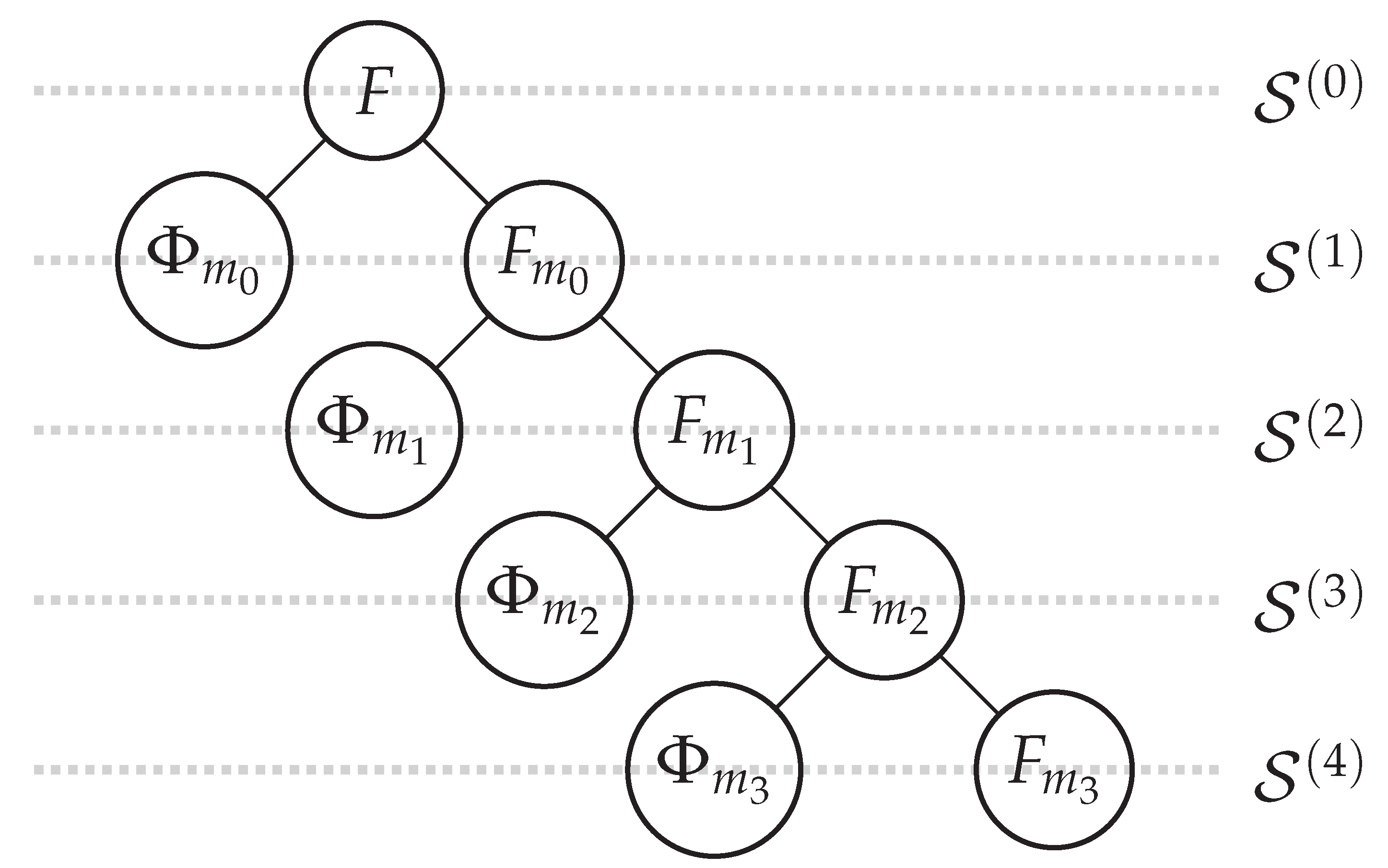
Figure 2.
Empirical Probability Density Distribution of Normalized FICO Scores for the Complete Dataset.
Figure 2.
Empirical Probability Density Distribution of Normalized FICO Scores for the Complete Dataset.
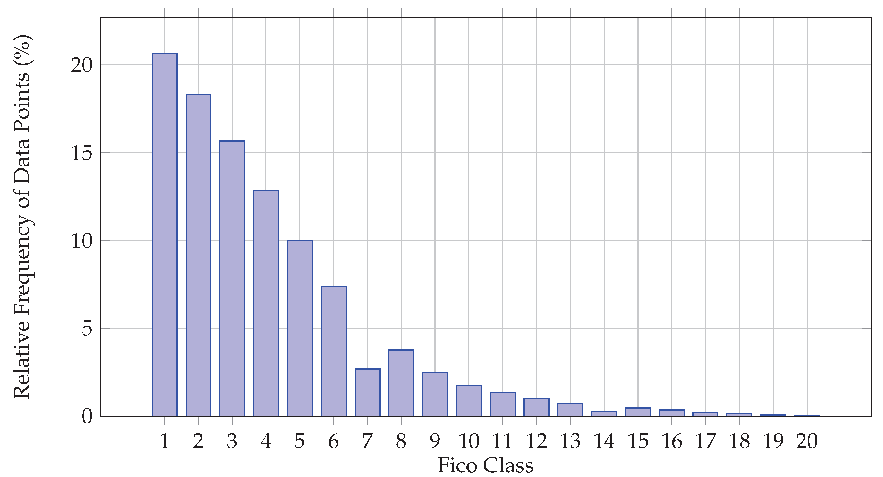
Figure 3.
PCA-Based Spatial Distribution for
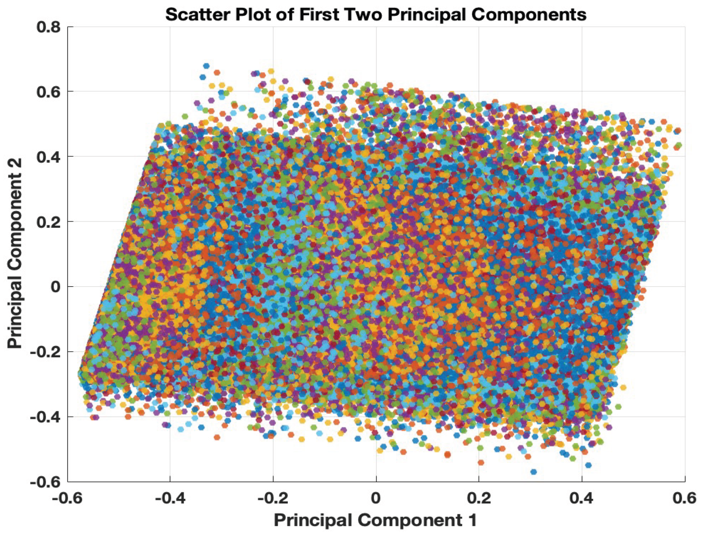
Figure 4.
PCA-Based Spatial Distribution for
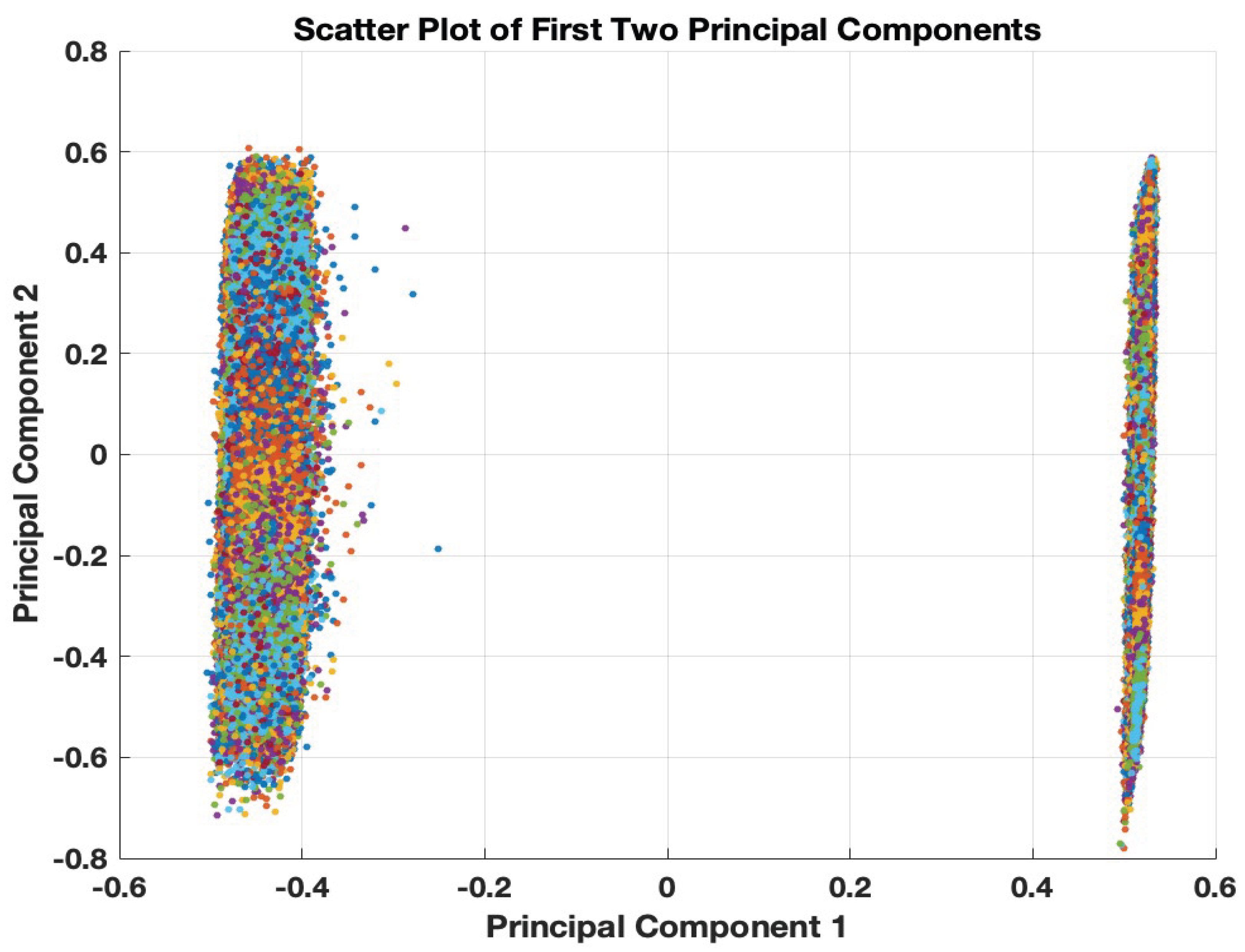
Figure 5.
Empirical Probability of Default per FICO Class for the Complete Dataset.

Figure 6.
Distance Layers per FICO Class

Figure 7.
Data Segmentation Process.
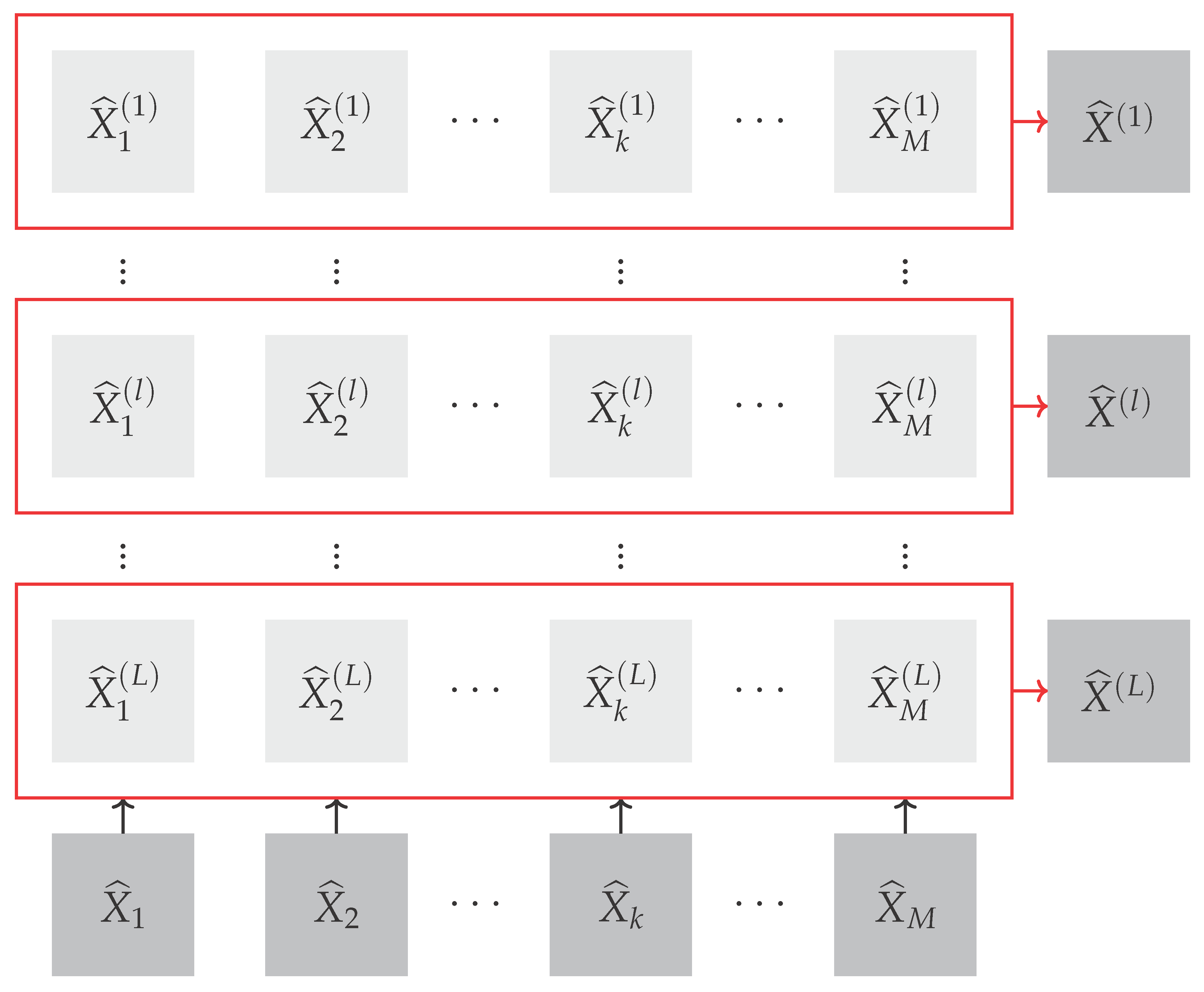
Table 1.
Descriptive Statistics of Regression Variables
| Min | Max | Normalized Mean | Normalized STD | |
|---|---|---|---|---|
| Annual Income (AI) | 10008 | 699587 | ||
| Debt-to-Income Ratio (DTI) | 0 | |||
| Revolving Balance (RB) | 0 | 1696796 | ||
| Revolving Utilization (RU) | 0 | 100 | ||
| Inquiries Last 6 Months (ILSM) | 0 | 5 | ||
| Delinquencies in the last 2 years (DLTY) | 0 | 29 | ||
| Months since the last Delinquency (MSLD) | 0 | 226 | ||
| Public Records (PR) | 0 | 61 | ||
| Total Current Balance-to-High Credit Ratio (BHCR) | 0 | 558 | ||
| Balance-to-Credit Limit on all trades (BCLA) | 0 | 204 | ||
| Total Revolving High Credit/Credit Limit (TRHC) | 100 | 1652700 | ||
| Public Record Bankruptcies (PRB) | 0 | 9 |
Table 2.
Probability Density Distribution of Normalized FICO Scores per Distance Layer.
| FICO Class | Layer 1 | Layer 2 | Layer 3 | Layer 4 | Layer 5 | Layer 6 | Layer 7 | Layer 8 | Layer 9 | Layer 10 | Layer 11 | Layer 12 | Layer 13 |
|---|---|---|---|---|---|---|---|---|---|---|---|---|---|
| 1 | 20.6428 | 20.6291 | 20.6291 | 20.6291 | 20.6291 | 20.6291 | 20.6291 | 20.6291 | 20.6291 | 20.6291 | 20.6291 | 20.6291 | 20.5769 |
| 2 | 18.2905 | 18.2789 | 18.2789 | 18.2789 | 18.2789 | 18.2789 | 18.2789 | 18.2789 | 18.2789 | 18.2789 | 18.2789 | 18.2789 | 18.2080 |
| 3 | 15.6701 | 15.6607 | 15.6607 | 15.6607 | 15.6607 | 15.6607 | 15.6607 | 15.6607 | 15.6607 | 15.6607 | 15.6607 | 15.6607 | 15.5857 |
| 4 | 12.8605 | 12.8536 | 12.8536 | 12.8536 | 12.8536 | 12.8536 | 12.8536 | 12.8536 | 12.8536 | 12.8536 | 12.8536 | 12.8536 | 12.8191 |
| 5 | 9.9807 | 9.9763 | 9.9763 | 9.9763 | 9.9763 | 9.9763 | 9.9763 | 9.9763 | 9.9763 | 9.9763 | 9.9763 | 9.9763 | 9.9257 |
| 6 | 7.3778 | 7.3757 | 7.3757 | 7.3757 | 7.3757 | 7.3757 | 7.3757 | 7.3757 | 7.3757 | 7.3757 | 7.3757 | 7.3757 | 7.3689 |
| 7 | 2.6776 | 2.6797 | 2.6797 | 2.6797 | 2.6797 | 2.6797 | 2.6797 | 2.6797 | 2.6797 | 2.6797 | 2.6797 | 2.6797 | 2.7010 |
| 8 | 3.7636 | 3.7647 | 3.7647 | 3.7647 | 3.7647 | 3.7647 | 3.7647 | 3.7647 | 3.7647 | 3.7647 | 3.7647 | 3.7647 | 3.7587 |
| 9 | 2.4886 | 2.4908 | 2.4908 | 2.4908 | 2.4908 | 2.4908 | 2.4908 | 2.4908 | 2.4908 | 2.4908 | 2.4908 | 2.4908 | 2.5262 |
| 10 | 1.7367 | 1.7396 | 1.7396 | 1.7396 | 1.7396 | 1.7396 | 1.7396 | 1.7396 | 1.7396 | 1.7396 | 1.7396 | 1.7396 | 1.7832 |
| 11 | 1.3366 | 1.3398 | 1.3398 | 1.3398 | 1.3398 | 1.3398 | 1.3398 | 1.3398 | 1.3398 | 1.3398 | 1.3398 | 1.3398 | 1.3505 |
| 12 | 0.9981 | 1.0016 | 1.0016 | 1.0016 | 1.0016 | 1.0016 | 1.0016 | 1.0016 | 1.0016 | 1.0016 | 1.0016 | 1.0016 | 1.0140 |
| 13 | 0.7299 | 0.7336 | 0.7336 | 0.7336 | 0.7336 | 0.7336 | 0.7336 | 0.7336 | 0.7336 | 0.7336 | 0.7336 | 0.7336 | 0.7343 |
| 14 | 0.2770 | 0.2811 | 0.2811 | 0.2811 | 0.2811 | 0.2811 | 0.2811 | 0.2811 | 0.2811 | 0.2811 | 0.2811 | 0.2811 | 0.3016 |
| 15 | 0.4529 | 0.4569 | 0.4569 | 0.4569 | 0.4569 | 0.4569 | 0.4569 | 0.4569 | 0.4569 | 0.4569 | 0.4569 | 0.4569 | 0.4589 |
| 16 | 0.3342 | 0.3383 | 0.3383 | 0.3383 | 0.3383 | 0.3383 | 0.3383 | 0.3383 | 0.3383 | 0.3383 | 0.3383 | 0.3383 | 0.3802 |
| 17 | 0.2023 | 0.2065 | 0.2065 | 0.2065 | 0.2065 | 0.2065 | 0.2065 | 0.2065 | 0.2065 | 0.2065 | 0.2065 | 0.2065 | 0.2054 |
| 18 | 0.1143 | 0.1186 | 0.1186 | 0.1186 | 0.1186 | 0.1186 | 0.1186 | 0.1186 | 0.1186 | 0.1186 | 0.1186 | 0.1186 | 0.1617 |
| 19 | 0.0484 | 0.0527 | 0.0527 | 0.0527 | 0.0527 | 0.0527 | 0.0527 | 0.0527 | 0.0527 | 0.0527 | 0.0527 | 0.0527 | 0.0962 |
| 20 | 0.0176 | 0.0220 | 0.0220 | 0.0220 | 0.0220 | 0.0220 | 0.0220 | 0.0220 | 0.0220 | 0.0220 | 0.0220 | 0.0220 | 0.0437 |
Table 3.
Run Parameters of GP Regression with 1 Gene
| Run Parameter | Value |
|---|---|
| Population Size | 100 |
| Maximum Generations | 50 |
| Input Variables | 4 |
| Training Instances | 20472 |
| Tournament Size | 10 |
| Elite Fraction | |
| Maximum Genes | 1 |
| Maximum Depth | 5 |
| Maximum Total Nodes | |
| Ephemeral Random Constants Probability | |
| Crossover Probability | |
| Mutation Probability |
Table 4.
GP Regression Training Accuracy Measures with 1 Gene
| - 4 Features | - 12 Features | |||||
|---|---|---|---|---|---|---|
| Layer | RMSE | MAE | RMSE | MAE | ||
| 1 | 0.0611 | 0.050 | 0.84 | 0.0597 | 0.050 | 0.85 |
| 2 | 0.0791 | 0.064 | 0.74 | 0.0681 | 0.056 | 0.81 |
| 3 | 0.0896 | 0.071 | 0.67 | 0.0736 | 0.060 | 0.77 |
| 4 | 0.0954 | 0.075 | 0.62 | 0.0814 | 0.065 | 0.72 |
| 5 | 0.1018 | 0.080 | 0.57 | 0.0834 | 0.066 | 0.71 |
| 6 | 0.1067 | 0.083 | 0.53 | 0.0928 | 0.073 | 0.64 |
| 7 | 0.1100 | 0.085 | 0.50 | 0.1072 | 0.087 | 0.52 |
| 8 | 0.1147 | 0.088 | 0.45 | 0.1204 | 0.098 | 0.40 |
| 9 | 0.1187 | 0.091 | 0.41 | 0.1275 | 0.099 | 0.32 |
| 10 | 0.1231 | 0.094 | 0.37 | 0.1236 | 0.093 | 0.36 |
| 11 | 0.1286 | 0.098 | 0.31 | 0.1232 | 0.091 | 0.37 |
| 12 | 0.1342 | 0.102 | 0.25 | 0.1266 | 0.091 | 0.33 |
| 13 | 0.1485 | 0.112 | 0.12 | 0.1265 | 0.092 | 0.36 |
Table 5.
GP Regression Testing Accuracy Measures with 1 Gene
| - 4 Features | - 12 Features | ||||||
| Layer | RMSE | MAE | RMSE | MAE | |||
| 1 | 0.0611 | 0.050 | 0.84 | 0.0598 | 0.050 | 0.85 | |
| 2 | 0.0791 | 0.064 | 0.74 | 0.0681 | 0.056 | 0.81 | |
| 3 | 0.0895 | 0.071 | 0.67 | 0.0737 | 0.060 | 0.77 | |
| 4 | 0.0954 | 0.075 | 0.62 | 0.0814 | 0.065 | 0.73 | |
| 5 | 0.1019 | 0.080 | 0.57 | 0.0835 | 0.066 | 0.71 | |
| 6 | 0.1067 | 0.083 | 0.53 | 0.0930 | 0.073 | 0.64 | |
| 7 | 0.1100 | 0.085 | 0.50 | 0.1071 | 0.087 | 0.52 | |
| 8 | 0.1149 | 0.088 | 0.45 | 0.1202 | 0.098 | 0.40 | |
| 9 | 0.1187 | 0.091 | 0.41 | 0.1279 | 0.099 | 0.32 | |
| 10 | 0.1229 | 0.094 | 0.37 | 0.1236 | 0.093 | 0.36 | |
| 11 | 0.1286 | 0.098 | 0.31 | 0.1229 | 0.090 | 0.37 | |
| 12 | 0.1344 | 0.102 | 0.25 | 0.1271 | 0.092 | 0.33 | |
| 13 | 0.1487 | 0.112 | 0.11 | 0.1264 | 0.092 | 0.36 | |
Table 6.
Gaussian SVM Regression Training Accuracy Measures
| - 4 Features | - 12 Features | ||||||
| Layer | RMSE | MAE | RMSE | MAE | |||
| 1 | 0.0004 | 0.046 | 0.86 | 0.0004 | 0.041 | 0.89 | |
| 2 | 0.0004 | 0.043 | 0.84 | 0.0004 | 0.041 | 0.87 | |
| 3 | 0.0005 | 0.042 | 0.82 | 0.0004 | 0.042 | 0.86 | |
| 4 | 0.0005 | 0.040 | 0.82 | 0.0004 | 0.044 | 0.83 | |
| 5 | 0.0005 | 0.040 | 0.80 | 0.0005 | 0.046 | 0.82 | |
| 6 | 0.0005 | 0.039 | 0.79 | 0.0005 | 0.047 | 0.80 | |
| 7 | 0.0005 | 0.038 | 0.79 | 0.0005 | 0.043 | 0.80 | |
| 8 | 0.0005 | 0.039 | 0.79 | 0.0005 | 0.037 | 0.81 | |
| 9 | 0.0005 | 0.039 | 0.78 | 0.0005 | 0.032 | 0.82 | |
| 10 | 0.0005 | 0.041 | 0.77 | 0.0005 | 0.033 | 0.81 | |
| 11 | 0.0005 | 0.042 | 0.76 | 0.0005 | 0.038 | 0.81 | |
| 12 | 0.0006 | 0.049 | 0.72 | 0.0005 | 0.047 | 0.77 | |
| 13 | 0.0008 | 0.076 | 0.49 | 0.0007 | 0.065 | 0.63 | |
Table 7.
Gaussian SVM Regression Testing Accuracy Measures
| - 4 Features | - 12 Features | ||||||
| Layer | RMSE | MAE | RMSE | MAE | |||
| 1 | 0.0012 | 0.047 | 0.86 | 0.0011 | 0.044 | 0.88 | |
| 2 | 0.0013 | 0.043 | 0.84 | 0.0012 | 0.043 | 0.86 | |
| 3 | 0.0014 | 0.042 | 0.82 | 0.0013 | 0.045 | 0.85 | |
| 4 | 0.0014 | 0.040 | 0.81 | 0.0014 | 0.046 | 0.82 | |
| 5 | 0.0015 | 0.040 | 0.80 | 0.0015 | 0.048 | 0.80 | |
| 6 | 0.0015 | 0.039 | 0.79 | 0.0015 | 0.050 | 0.79 | |
| 7 | 0.0015 | 0.039 | 0.79 | 0.0015 | 0.046 | 0.79 | |
| 8 | 0.0015 | 0.039 | 0.79 | 0.0015 | 0.040 | 0.79 | |
| 9 | 0.0016 | 0.040 | 0.77 | 0.0014 | 0.034 | 0.81 | |
| 10 | 0.0016 | 0.041 | 0.76 | 0.0015 | 0.036 | 0.79 | |
| 11 | 0.0016 | 0.043 | 0.76 | 0.0015 | 0.040 | 0.79 | |
| 12 | 0.0018 | 0.050 | 0.71 | 0.0016 | 0.050 | 0.75 | |
| 13 | 0.0024 | 0.078 | 0.48 | 0.0021 | 0.070 | 0.59 | |
Table 8.
MLP Regression Training Accuracy Measures
| - 4 Features | - 12 Features | ||||||
| Layer | RMSE | MAE | RMSE | MAE | |||
| 1 | 0.0004 | 0.047 | 0.86 | 0.0004 | 0.043 | 0.88 | |
| 2 | 0.0004 | 0.045 | 0.84 | 0.0004 | 0.044 | 0.87 | |
| 3 | 0.0005 | 0.045 | 0.83 | 0.0004 | 0.045 | 0.86 | |
| 4 | 0.0005 | 0.043 | 0.82 | 0.0004 | 0.046 | 0.84 | |
| 5 | 0.0005 | 0.043 | 0.81 | 0.0005 | 0.049 | 0.83 | |
| 6 | 0.0005 | 0.044 | 0.80 | 0.0005 | 0.048 | 0.82 | |
| 7 | 0.0005 | 0.043 | 0.80 | 0.0005 | 0.045 | 0.82 | |
| 8 | 0.0005 | 0.044 | 0.80 | 0.0005 | 0.041 | 0.82 | |
| 9 | 0.0005 | 0.044 | 0.78 | 0.0004 | 0.036 | 0.83 | |
| 10 | 0.0005 | 0.045 | 0.78 | 0.0005 | 0.038 | 0.81 | |
| 11 | 0.0005 | 0.047 | 0.77 | 0.0005 | 0.042 | 0.81 | |
| 12 | 0.0005 | 0.054 | 0.72 | 0.0005 | 0.051 | 0.77 | |
| 13 | 0.0008 | 0.080 | 0.49 | 0.0007 | 0.069 | 0.65 | |
Table 9.
MLP Regression Testing Accuracy Measures
| - 4 Features | - 12 Features | ||||||
| Layer | RMSE | MAE | RMSE | MAE | |||
| 1 | 0.0012 | 0.047 | 0.86 | 0.0011 | 0.044 | 0.88 | |
| 2 | 0.0013 | 0.046 | 0.84 | 0.0012 | 0.046 | 0.86 | |
| 3 | 0.0014 | 0.045 | 0.82 | 0.0013 | 0.047 | 0.84 | |
| 4 | 0.0014 | 0.043 | 0.82 | 0.0014 | 0.048 | 0.83 | |
| 5 | 0.0014 | 0.044 | 0.81 | 0.0014 | 0.051 | 0.81 | |
| 6 | 0.0015 | 0.044 | 0.80 | 0.0014 | 0.050 | 0.81 | |
| 7 | 0.0015 | 0.043 | 0.80 | 0.0015 | 0.047 | 0.80 | |
| 8 | 0.0015 | 0.044 | 0.79 | 0.0015 | 0.043 | 0.80 | |
| 9 | 0.0015 | 0.045 | 0.78 | 0.0014 | 0.038 | 0.81 | |
| 10 | 0.0016 | 0.046 | 0.77 | 0.0015 | 0.040 | 0.79 | |
| 11 | 0.0016 | 0.047 | 0.77 | 0.0015 | 0.044 | 0.79 | |
| 12 | 0.0017 | 0.055 | 0.72 | 0.0016 | 0.053 | 0.75 | |
| 13 | 0.0024 | 0.081 | 0.48 | 0.0021 | 0.071 | 0.61 | |
Table 10.
RBFN Regression Training Accuracy Measures
| - 4 Features | - 12 Features | ||||||
| Layer | RMSE | MAE | RMSE | MAE | |||
| 1 | 0.0004 | 0.048 | 0.85 | 0.0004 | 0.046 | 0.87 | |
| 2 | 0.0005 | 0.057 | 0.78 | 0.0005 | 0.053 | 0.82 | |
| 3 | 0.0006 | 0.060 | 0.74 | 0.0005 | 0.058 | 0.78 | |
| 4 | 0.0006 | 0.059 | 0.73 | 0.0005 | 0.061 | 0.75 | |
| 5 | 0.0006 | 0.061 | 0.70 | 0.0006 | 0.065 | 0.72 | |
| 6 | 0.0006 | 0.061 | 0.69 | 0.0006 | 0.070 | 0.68 | |
| 7 | 0.0006 | 0.060 | 0.69 | 0.0007 | 0.079 | 0.60 | |
| 8 | 0.0006 | 0.060 | 0.69 | 0.0008 | 0.089 | 0.49 | |
| 9 | 0.0006 | 0.061 | 0.67 | 0.0008 | 0.087 | 0.45 | |
| 10 | 0.0006 | 0.062 | 0.66 | 0.0008 | 0.080 | 0.50 | |
| 11 | 0.0006 | 0.061 | 0.66 | 0.0008 | 0.081 | 0.48 | |
| 12 | 0.0007 | 0.065 | 0.62 | 0.0008 | 0.085 | 0.44 | |
| 13 | 0.0009 | 0.091 | 0.36 | 0.0008 | 0.085 | 0.44 | |
Table 11.
RBFN Regression Testing Accuracy Measures
| - 4 Features | - 12 Features | ||||||
| Layer | RMSE | MAE | RMSE | MAE | |||
| 1 | 0.0012 | 0.048 | 0.85 | 0.0012 | 0.046 | 0.87 | |
| 2 | 0.0015 | 0.057 | 0.78 | 0.0014 | 0.053 | 0.82 | |
| 3 | 0.0017 | 0.060 | 0.74 | 0.0015 | 0.058 | 0.78 | |
| 4 | 0.0017 | 0.059 | 0.73 | 0.0016 | 0.061 | 0.75 | |
| 5 | 0.0018 | 0.061 | 0.70 | 0.0017 | 0.065 | 0.72 | |
| 6 | 0.0018 | 0.061 | 0.69 | 0.0018 | 0.070 | 0.68 | |
| 7 | 0.0018 | 0.061 | 0.69 | 0.0021 | 0.079 | 0.60 | |
| 8 | 0.0018 | 0.060 | 0.69 | 0.0023 | 0.089 | 0.49 | |
| 9 | 0.0019 | 0.061 | 0.67 | 0.0024 | 0.087 | 0.45 | |
| 10 | 0.0019 | 0.062 | 0.66 | 0.0023 | 0.080 | 0.50 | |
| 11 | 0.0019 | 0.061 | 0.65 | 0.0023 | 0.081 | 0.48 | |
| 12 | 0.0020 | 0.065 | 0.62 | 0.0024 | 0.085 | 0.44 | |
| 13 | 0.0026 | 0.091 | 0.36 | 0.0025 | 0.085 | 0.44 | |
Table 12.
Regression Tree Training Accuracy Measures
| - 4 Features | - 12 Features | ||||||
| Layer | RMSE | MAE | RMSE | MAE | |||
| 1 | 0.0004 | 0.048 | 0.86 | 0.0004 | 0.045 | 0.87 | |
| 2 | 0.0005 | 0.056 | 0.79 | 0.0004 | 0.052 | 0.83 | |
| 3 | 0.0006 | 0.061 | 0.74 | 0.0005 | 0.055 | 0.81 | |
| 4 | 0.0006 | 0.063 | 0.71 | 0.0005 | 0.057 | 0.78 | |
| 5 | 0.0006 | 0.066 | 0.67 | 0.0005 | 0.059 | 0.76 | |
| 6 | 0.0006 | 0.066 | 0.66 | 0.0006 | 0.062 | 0.73 | |
| 7 | 0.0007 | 0.068 | 0.63 | 0.0006 | 0.063 | 0.70 | |
| 8 | 0.0007 | 0.070 | 0.62 | 0.0007 | 0.073 | 0.58 | |
| 9 | 0.0007 | 0.071 | 0.59 | 0.0007 | 0.068 | 0.61 | |
| 10 | 0.0007 | 0.072 | 0.57 | 0.0007 | 0.071 | 0.56 | |
| 11 | 0.0007 | 0.073 | 0.57 | 0.0007 | 0.073 | 0.55 | |
| 12 | 0.0007 | 0.075 | 0.53 | 0.0008 | 0.078 | 0.51 | |
| 13 | 0.0008 | 0.086 | 0.44 | 0.0008 | 0.079 | 0.53 | |
Table 13.
Regression Tree Testing Accuracy Measures
| - 4 Features | - 12 Features | ||||||
| Layer | RMSE | MAE | RMSE | MAE | |||
| 1 | 0.0013 | 0.049 | 0.85 | 0.0012 | 0.046 | 0.87 | |
| 2 | 0.0015 | 0.056 | 0.78 | 0.0014 | 0.053 | 0.82 | |
| 3 | 0.0017 | 0.062 | 0.73 | 0.0015 | 0.056 | 0.80 | |
| 4 | 0.0018 | 0.064 | 0.70 | 0.0016 | 0.058 | 0.77 | |
| 5 | 0.0019 | 0.067 | 0.66 | 0.0016 | 0.061 | 0.75 | |
| 6 | 0.0019 | 0.068 | 0.64 | 0.0017 | 0.063 | 0.72 | |
| 7 | 0.0020 | 0.070 | 0.62 | 0.0018 | 0.064 | 0.68 | |
| 8 | 0.0021 | 0.071 | 0.60 | 0.0022 | 0.075 | 0.56 | |
| 9 | 0.0021 | 0.073 | 0.57 | 0.0021 | 0.070 | 0.59 | |
| 10 | 0.0022 | 0.074 | 0.55 | 0.0022 | 0.073 | 0.54 | |
| 11 | 0.0022 | 0.074 | 0.54 | 0.0022 | 0.075 | 0.53 | |
| 12 | 0.0023 | 0.076 | 0.51 | 0.0023 | 0.080 | 0.48 | |
| 13 | 0.0026 | 0.088 | 0.40 | 0.0024 | 0.081 | 0.49 | |
Table 14.
Layer-wise Frequency Values for the Independent Regression Variables AI, DTI, RB, and RU.
| Layer | AI | DTI | RB | RU | |
|---|---|---|---|---|---|
| 1 | 0.1278 | 0.1051 | 0.3345 | 0.4326 | 0.8401 |
| 2 | 0.1234 | 0.0588 | 0.2762 | 0.5416 | 0.7309 |
| 3 | 0.1340 | 0.1127 | 0.1706 | 0.5827 | 0.6476 |
| 4 | 0.1689 | 0.0611 | 0.1917 | 0.5783 | 0.6091 |
| 5 | 0.1819 | 0.0389 | 0.2827 | 0.4964 | 0.5522 |
Table 15.
Layer-wise Frequency Values for the Independent Regression Variables AI, DTI, RB, RU, ILSM, DLTY, MSLD, PR, BHCR, BCLA, TRHC, PRB.
Table 15.
Layer-wise Frequency Values for the Independent Regression Variables AI, DTI, RB, RU, ILSM, DLTY, MSLD, PR, BHCR, BCLA, TRHC, PRB.
| Layer | AI | DTI | RB | RU | ILSM | DLTY | MSLD | PR | BHCR | BCLA | TRHC | PRB | |
|---|---|---|---|---|---|---|---|---|---|---|---|---|---|
| 1 | 0.0530 | 0.0236 | 0.0170 | 0.3423 | 0.0072 | 0.0137 | 0.2480 | 0.0340 | 0.0295 | 0.1348 | 0.0262 | 0.0707 | 0.8339 |
| 2 | 0.0551 | 0.0101 | 0.0178 | 0.4339 | 0.0302 | 0.0119 | 0.2134 | 0.0356 | 0.0403 | 0.0634 | 0.0095 | 0.0788 | 0.7881 |
| 3 | 0.0255 | 0.0154 | 0.0255 | 0.2916 | 0.0303 | 0.0178 | 0.2357 | 0.0285 | 0.0932 | 0.0499 | 0.0386 | 0.1479 | 0.7439 |
| 4 | 0.0287 | 0.0143 | 0.0208 | 0.2237 | 0.0523 | 0.0186 | 0.2502 | 0.0380 | 0.0222 | 0.1333 | 0.0545 | 0.1434 | 0.6755 |
| 5 | 0.0904 | 0.0149 | 0.0194 | 0.2676 | 0.0284 | 0.0306 | 0.2220 | 0.0172 | 0.0845 | 0.0635 | 0.0411 | 0.1203 | 0.6949 |
Table 16.
GP-Based Symbolic Regression Expressions for and .
| Feature Set | Expression |
|---|---|
Disclaimer/Publisher’s Note: The statements, opinions and data contained in all publications are solely those of the individual author(s) and contributor(s) and not of MDPI and/or the editor(s). MDPI and/or the editor(s) disclaim responsibility for any injury to people or property resulting from any ideas, methods, instructions or products referred to in the content. |
© 2024 by the authors. Licensee MDPI, Basel, Switzerland. This article is an open access article distributed under the terms and conditions of the Creative Commons Attribution (CC BY) license (http://creativecommons.org/licenses/by/4.0/).
Copyright: This open access article is published under a Creative Commons CC BY 4.0 license, which permit the free download, distribution, and reuse, provided that the author and preprint are cited in any reuse.


