Use of Chitosan and Chitosan-Magnetite Spheres for Arsenic Groundwater Removal. Factorial Designs as Tools to Calculate the Efficiency of Removal

The lack of access to drinking water is a problem that affects many towns in the Province of Santa Fe. Many people affected by this situation use groundwater for consumption, cooking, and irrigation. In this work, a colorimetric analytical technique is used to quantify arsenic. It is sufficiently sensitive, simple, and economical to apply to the towns of interest. This work synthesized a hybrid sorbent in the form of magnetite-chitosan spheres (M-Q). The sorption capacity of this new sorbent for As removal was 270% greater than that of chitosan spheres (Q), which was 30%. Another advantage of this hybrid sorbent is the capability of being sep-arated by its magnetic properties. The work was done with groundwater (Andino, Province of Santa Fe) with high conductivity (12.1 µS/cm), hardness (1125 mg/L CaCO3), and an As(V) concentration of 265 µg/L. The removal capacity from groundwater was optimized using a composite factorial design, and for the conditions of mass 0.49 g, pH 5.24, and contact time of 81.23 min, it was found to be 81%.

Keywords:

Subject: Chemistry and Materials Science - Biomaterials

1. Introduction

Water is a natural and indispensable resource, it is of fundamental importance, since without it, life on the planet could not exist(Benítez et al., 2021) Currently, human exposure to high concentrations of arsenic (As) present in groundwater/aquifers is one of the most widespread environmental problems in many countries (Singh et al., 2015) The International Agency for Research on Cancer (IARC) classifies As in group I (sufficient evidence of carcinogenicity in humans)(Loomis et al., 2018), while the United States Environmental Protection Agency (USEPA) describes it as a group A human carcinogen(Abernathy et al., 1989) As is a metalloid that is widely distributed in the environment in water, rocks, soil, and air. It contaminates plants, animals, and consequently, the food consumed by humans. As in water is present in its organic and inorganic forms, being the inorganic form the most common. As has different oxidation states: arsenites (AsO₃^3-) and arsenates (AsO₄^3-) are widespread in water bodies. The toxicity of As increases considerably with the reduction of its oxidation state from As(V) to As(III), additionally the organic forms are less toxic than the inorganic ones.

As represents a global and regional problem: in Argentina, the presence of As in the environment and specifically in water for human consumption is basically due to natural factors with some anthropogenic contribution (Litter, 2018; O’reilly et al., 2010). Detection and quantification of As in the aquifers of Argentina is the subject of intense scientific activity. The purpose of these studies is to define regions based on the degree of contamination to have a deep understanding of the dimensions of this problem and promote initiatives that provide improvement solutions(Marchetti et al., 2021). The World Health Organization (WHO) recommends 0.01 mg/L as the maximum permitted level of As for human and agricultural use to reduce the negative impacts of this metalloid on human health (Edition, 2011; UNICEF, 2018). In Argentina, the permitted value for drinking water varies according to the provinces. The allowed limit of As in Santa Fe is 0.05 mg/L (Corey et al., 2005; ENRRES, 2016). Concentrations in groundwater of western Santa Fe province and the city of Córdoba, exceed 0.1 and 0.5 mg/L, respectively (Bardach et al., 2015). Different treatment technologies have been used to reduce its concentration and avoid its harmful effects on the environment and people's health, which are being constantly studied and tested internationally (Sardar et al., 2021) and are based on physical-chemical methods (oxidation/reduction, coagulation-filtration, precipitation, adsorption and ion exchange, solid/liquid separation, physical exclusion, membrane technologies), as well as biological methods (phytoremediation, electrokinetic treatment). All these methods have advantages and disadvantages. For example, reduction-precipitation and coagulation-flocculation are the most common methods. However, their cost is high because they require the participation of chemical agents (which cannot be reused), and they generate toxic sludge that is difficult to handle and treat. In addition, the high cost of many of these conventional water methods is not cost-effective, especially in small communities. The need for economical and effective methods for eliminating different pollutants resulted in the development of new separation technologies, such as remediation. The technique uses sorbents such as algae, and agro-industry waste (Abanto Pérez & Reyes Benites, 2021; Cuizano et al., 2009; García et al., 2023; Paredes Ramirez & Segura Acosta, 2021), biopolymers, or mixtures of biopolymers with metal oxides (hybrid sorbents) (Silva Lizama, 2023).

The reverse Osmosis technique deserves a separate paragraph. Most of the towns near the central cities (Santa Fe, the capital, and Rosario) do not have drinking water networks due to the nonexistence of aqueducts. This long-standing lack of infrastructure is not related to the lack of water since the Paraná River is large and long enough to supply the central drinking water generation plants; the problem lies in the fact that drinking water does not reach the towns, so they must source themselves from groundwaters that have high hardness, significant contaminants and As in variable quantities (often exceeding the permitted limits). For this reason, reverse osmosis plays a preponderant role. Most towns use it (El Trebol, San Jorge, Piamonte, Roldán, Andino, etc.). This technique provides the population with immediate drinking water, but some drawbacks exist. The main one is that the wastewater, which contains 90-95% of the ions in groundwater, is stored in large tanks or basins and, in the worst case, returned to the groundwater. In this way, the problem of providing drinking water is solved immediately, but the concentration of contaminants in the groundwater (including As(V)) remains unresolved. Several studies have been carried out in recent years, with hybrid materials to eliminate As from water (Martínez-Cabanas, 2017). These hybrid sorbent materials use chitosan (Q) as a support or matrix for metal oxide (such as magnetite (M), maghemite, and others).

This work is a continuation of a previous one (Batistelli et al., 2023). Here, it is demonstrated that incorporating M into the Q gel to generate the hybrid sorbent Q-M increases the As sorption percentage and gives more mechanical stability to the Q-M sorbent during the stirring/reaction time. The hybrid sorbent Q-M removed 81% of the initial As in high-salinity groundwater, and, therefore, high ionic strength. Finally, the optimal experimental conditions for As sorption (pH, time, and mass of the hybrid sorbent Q-M) were obtained by response surface factorial designs, which significantly reduced the total number of experiments, and, at the same time, demonstrated that all the selected variables significantly affected the As sorption percentage (response studied).

2. Materials and Methods

2.1. Reagents

Inorganic Reagents:

Hydrochloric acid 36% W/W, δ = 1.18 g/mL (Cicarelli), Sulfuric acid 98% W/W, δ = 1.84 g/mL (Cicarelli), Nitric acid (Cicarelli) 65% W/W, δ = 1.53 g/mL, Sodium hydroxide (Cicarelli), Sodium nitrate (Anedra), Ammonium hydroxide 25–30% W/V, δ = 8.9 g/mL (Cicarelli), Hydroxylamine hydrochloride (Anedra).

Reagents provided by GT Laboratory (GMP, ISO 9001:2008 and ISO 13485: 2003 standards): KI 0.1 M, SnCl₂ 0.15 M, Zn (As-free) Shots, Lead Acetate Filters, Silver Diethyldithiocarbamate (DDCAg), Pyridine Solution p.a. (BiopacK) 0.982 g/ml, As(V) standard 100 mg/L. Fe(III) standard 1000 ug/L (ChemLab). Ferrous sulfate heptahydrate FeSO₄.7H₂O salts were used as a source of Fe²⁺ ions, and ferric chloride hexahydrate FeCl₃.6H₂O as a source of Fe³⁺ ions, which were provided by Biopack (Fe²⁺) and Cicarelli (Fe³⁺), in analytical grade.

Organic Reagents:

Acetic acid 99.5% W/W, δ = 1.67 g/mL (Cicarelli), Chitosan (Parafarm), degree of acetylation of 98% and Mv = 1.61 x 10⁵ g/mol, pH buffer solutions (4.0, 7.0 and 10.0) (Cicarelli), Antimony and potassium tartrate (Mallinckrodt), ortho-phenathroline (Cicarelli), Amonium Acetate (Biopack).

Commercial Kits:

Commercial kit for the detection of total As (ARSENICOAQAssay - GTLab), Commercial kit for the detection of total nitrites (Hanna Instruments), Commercial kit for the determination of total hardness (LQT AQAssay).

Control of Physical-Chemical Parameters

A Hanna Instruments 8519 pH meter and a Hanna Instruments Dist 4 conductivity meter were used to measure the pH, temperature, and conductivity of solutions and samples. A Cole - Parmer® 8891E – DTH sonicator bath was used. The groundwater was characterized using a GTLab (AQAssay) kit.

2.2. Sorbent Synthesis

2.2.1. Synthesis of Chitosan (Q) Spheres

4.0 g of Q was dissolved in 100.0 mL of acetic acid (4.0% W/V at 40°C). The solution was homogenized with a magnetic stirrer for 24 h, and slowly dripped onto NaOH 4M, with gentle and constant stirring. The obtained spheres were incubated for 24 h in the sodium hydroxide solution to complete the gelling process and washed with enough distilled water to neutral pH. Finally, the Q spheres were dried at room temperature (25°C) until constant weight and stored in caramel-colored glass containers.

2.2.2. Magnetite (M) Synthesis

All synthesis was carried out in an inert nitrogen atmosphere: 7.84 g of Fe(NH₄)₂(SO₄)₂.6H₂O and 10.80 g of FeCl₃.6H₂O were weighed and dissolved in 200 mL of distilled water (deoxygenated) to prepare 0.1M and 0.2M solution in Fe(II) and Fe(III), respectively. To this solution, 70 mL ammonium hydroxide (20% V/V) was added, with stirring and under a hood, up to pH 9.0, observing the formation of a black suspension which was incubated at 80°C for 30 min. The solid obtained was separated by decantation and washed with distilled water (deoxygenated) until neutral pH. The solid obtained was dried at room temperature until constant weight, ground to powder, and stored in a desiccator in a nitrogen atmosphere.

The magnetite synthesis reaction is shown in Equation (1):

Fe(NH₄)₂(SO₄)₂ + 2FeCl₃ + 8NH₄OH → Fe₃O₄ + 4H₂O +2(NH₄)₂SO₄ + 6NH₄Cl

(1)

Theoretical mass = 4.64 g; mass obtained = 4.60 g and yield = 98.9%.

2.2.3. Synthesis of Magnetite–Chitosan (M-Q) Spheres

For this, 4.0 g of Q was dissolved in 100.0 mL of acetic acid (4.0% W/V at 40°C). The solution was mixed with 0,702 g of M, stirred, and homogenized in a sonicator (40 min). The mixture was slowly dripped onto a 4M sodium hydroxide solution with gentle stirring, observing the gelling of the drops as they fell. The mixed spheres obtained were left to rest in the sodium hydroxide solution for 24 h to complete the gelling process. They were left at room temperature (25°C) until constant weight and stored in caramel-colored glass containers.

2.3. Characterization of Sorbent Material

Three different assays, described below, were performed to characterize sorbent spheres.

2.3.1. Determination of Zero-Charge pH (pHzc)

To determine the pH_zc of both synthesized sorbent, the Muller method was followed (Mular & Roberts, 1966). Different solutions with pH values in the range of 1–9 were prepared, using H₂SO₄ and NaOH. 50 mL of each solution was placed in a beaker and the initial pH (pH₀) was measured. The same mass of sorbent (0.1 g) was added to each one. After 10 minutes 3.45 g of NaNO₃ was added to regulate the ionic strength of the system to a common value of 0.1 M and left to stir for 24 h, after which the final pH (pH_f) was recorded, calculating the ∆pH value as the difference between pH₀ and pH_f. The pH_zc value is determined from the ∆pH vs pH₀ graph, as the point at which the graph cuts the x-axis (pH₀).

2.3.2. Iron Percentage Determination for M–Q Spheres

10 spheres of Q-M, with a mass of 0.0262 g, were placed in a beaker with 2 mL concentrated HCl and 2 mL concentrated HNO₃, and heated in a hood, until total dissolution. The result solution was cooled to room temperature, and the volume was adjusted to 4 mL with distillate water and diluted 25 times with distilled water. For iron determination, the ortho-phenanthroline method was used (Association, 1926): 1 mL of this solution was added with 1 mL of 1M acetate ammonium, 1 mL of 10% hydroxylamine hydrochloride, and 10 mL of solution 0.03% ortho-phenanthroline, and dilute exactly to 50 mL with distilled water. After 45 min, absorbance was determined spectrophotometrically at 510 nm.

The method allows the determination of total iron, after reducing the Fe(III) present in the sample to Fe(II), with hydroxylamine. Reduction is achieved using an excess hydroxylamine, according to Equation (2):

4Fe³⁺ + 2NH₂OH → 4Fe²⁺ + N₂O + 4H⁺ + H₂O

(2)

Then, Fe(II) reacts with the color reagent, ortho-phenanthroline, giving a red-orange complex, according to Equation (3):

3C₁₂H₈N₂ + Fe²⁺ → [Fe(C₁₂H₈N₂)₃]²⁺

(3)

whose intensity is measured at 510 nm. The absorbance obtained is directly proportional to the concentration of iron. The determination was made in duplicate and contrasted with a calibration curve.

2.3.3. Powder X-Ray Diffraction (XRD)

This characterization technique identifies the crystalline planes of a periodic material (from a structural point of view) and is based on Bragg's law. A beam of X-rays generated from an anode is incident on the sample, which interacts with the outer electrons of the atoms present in the different planes of the sample (Reventós et al., 2012). This interaction produces a diffraction of the incident wave captured by a detector. In addition, the X-rays emitted from nearby atoms interfere with each other, constructively or destructively. For this interference to be constructive, the angle of incidence of the X-rays must satisfy Bragg's Law for each family of planes (the radiation emitted by different atoms must be proportional to 2θ (Waseda et al., 2011). Mathematically, it is expressed in Equation (4):

𝑛 𝜆 = 2𝑑 sin𝜃

(4)

where n = whole number (reflects the angle between the incident and scattered beams), λ = wavelength of the incident X-rays, d = interplanar distance, and θ = angle between incident rays and scattering planes. In the powder analysis, the X-rays are incident in different directions by moving the angle of incidence to identify all the possible crystalline planes, that can be found in the sample, Figure 1. The sorbent material in spheres was pulverized in a mortar, while the synthesized Q and M were analyzed without prior treatment. The diffractograms were obtained with a D2 Phaser X-Ray Diffractometer with a second-generation detector, applying the parameters in Table 1.

2.4. As(V) Quantification

For As quantification, an economical, sensitive, and accepted spectrophotometric method by current standards has been selected (Wastewater, 2017). This method is based on the reduction of As(V) to As(III) with Zn in HCl media, generating arsine (AsH₃), according to Equation (5). Arsine reacts with silver diethyldithiocarbamate (DDCAg) in pyridine (Pyr) solution to give a pink complex, Equation (6), whose absorption maximum is 530 nm. The stability of the As(DDCAg)₃ complex is 1 h at room temperature.

4Zn + 8H₃O⁺ + H₃AsO₄ → AsH₃ + 12H₂O + 4Zn²⁺

(5)

AsH₃ + 6DDCAg + 3Pyr → 6Ag⁺ + As(DDCAg)₃ + 3DDC^- + 3PyrH⁺

(6)

The equipment used for the determination of As is shown in the Figure 2. The sample containing As(V) is placed in the conic flask, with concentrate HCl, and SnCl₂ and KI (used as auxiliary reducers) for 15 min, after that, Zn powder is added an AsH₃ is generated, passing through cotton soaked embedded with a lead acetate solution, to retain SH₂, an interferent in this method. Finally reacts with DDCAg dissolved in Pyr to form a soluble red complex, whose color intensity is proportional to the arsenic content in the sample. The resulting mixture was allowed to react for 40 min, and then absorption spectra measurements were performed at 530 nm. The complete spectrum for the colored complex is shown in supplementary material.

The equipment must be placed under a fume hood due to the release of hydrogen, arsine, and pyridine vapors. The quantities and order of addition of the reagents used in the protocol are summarized in Table 2.

An hermetically sealed glass cuvette with an optical path length of 1.0 cm was used for each measurement. The absorbance value of a blank solution was subtracted from each absorbance value for the concentrations under study. The absorbance values at 530 nm were considered for constructing the calibration curve.

A calibration curve was realized to determine the molar absorptivity of the complex in groundwater and to verify the linearity of the system.

Regression analysis, using the least squares method, allows obtaining the equation of the straight line that best fits the experimental data and specifying the uncertainty associated with its use. When using the least squares method, two assumptions must be made: there is a linear relationship between the measured variable (y) and the concentration of the analyte (x). The mathematical relationship that describes this relationship is called a regression model and is represented by the Equation (7):

y = B + Ax

(7)

where B is the ordinate at the origin and A is the slope.

Deviations of experimental results from the straight line are due to measurement errors; it is assumed that there are no errors in the values of x. The deviation of each experimental result (y_i) from the straight line is called the residual. The straight line obtained by the least squares method is the one that minimizes the sum of the squares of the residuals for all points. In addition to providing the straight line that best fits the experimental data, the method also provides the standard deviation of the slope (S_A), intercept (S_B), and regression (S_R).

Linear regression: Univariate Calibration Line

Measurement of the response of the standards: once the standards of known concentration were prepared, their analytical responses were measured, including the replicas. To perform the linear regression analysis, it was necessary to calculate the slope (A) and the intercept (B), Equations (8) and (9), of the line fitted to the Equation (7).

A = \frac{Q_{x y}}{Q_{x x}} = \frac{\sum_{i = 1}^{m} {(y_{i} - \bar{y})}^{2}}{\sum_{i = 1}^{m} {(x_{i} - \bar{x})}^{2}}

(8)

B = \bar{y} - A \bar{x}

(9)

Equation (10) was used to calculate the standard deviation of the regression residuals (S_y/x).

S_{y / x} = \sqrt{\frac{\sum_{i = 1}^{m} {(y_{i} - {\hat{y}}_{i})}^{2}}{m - 2}}

(10)

where y_i is the experimental response of each calibration pattern and ŷ_i represents the estimated response at each point, that is, ŷ_i = A x_i + B. In Equation (10), m – 2 degrees of freedom are used, since there are m data available, and 2 estimated parameters in the regression (A and B). In this case, six standard solutions of increasing concentration were used and each of them was measured in triplicate (m = 18).

The parameters A, B and sample concentration (x_inc) must be reported with their degree of uncertainty, otherwise they have no analytical value. The related uncertainties (standard deviations) were calculated with Equations (11)–(13).

S_{A} = \frac{S_{y / x}}{\sqrt{Q x x}}

(11)

S_{B} = S_{y / x} \sqrt{\frac{1}{m} + \frac{\bar{x}}{Q_{x x}}}

(12)

S (x_{i n c}) = \frac{S_{y / x}}{A} \sqrt{\frac{1}{n} + \frac{1}{m} + \frac{{(x_{i n c} - \bar{x})}^{2}}{Q_{x x}}}

(13)

In Equations (11)–(13), m is the total number of calibration standards, n is the number of replicates of the unknown sample,

\bar{x}

is the arithmetic mean, (x_inc) the predicted value of the concentration, and S(x_inc) its associated standard deviation value. The meaning of Q_xx was defined in Equation (8).

The detection limit (DL) was calculated based on the standard deviation of the predicted concentration for a blank sample, S(x_inc). If a sample without analyte (x_inc = 0) is analyzed in triplicate, Equation (13) reduces to Equation (14):

L D = 3.3 \frac{s_{y / x}}{A} \sqrt{\frac{1}{3} + \frac{1}{18} + \frac{{(- \bar{x})}^{2}}{Q_{x x}}}

(14)

The limit of quantification (LQ) was calculated as indicated by Equation (15).

L Q = \frac{L D * 10}{3.3}

(15)

2.5. Experimental Design Applied to As(V) Sorption

A central composite rotating surface design (CCD) model was chosen. Three factors were considered independent variables: time, pH, and sorbent mass, at two levels and four repetitions of the central point. Table 3A and Table 3B summarize the ranges and levels of the factors studied.

The total number of experiments in this model, 18, is calculated as 2k + 2k + n (k is the number of factors and n is the repetitions of the central point). The Design-Expert 11 program was used to prepare the design.

The percentage of As(V) sorption (%R) of each experiment was selected as response and calculated with Equation (16)

% R = \frac{C_{0} - C_{f}}{C_{0}} x 100

(16)

where C₀ is the initial concentration (265 µg/L), and C_f is the final concentration, at time t, of As(V), expressed in mg/L. The temperature and working volume were 25°C and 200 mL, respectively. A second-order polynomial was used to study the percentage of As(V) removal and recognize the most relevant terms of the model. The complete quadratic model is presented in Equation (17).

Y = β_{0} + \sum_{i = 1}^{k} β_{j} X_{i} + \sum_{i = 1}^{k} β_{i i} X_{i}^{2} + \sum_{i = 1}^{k} β_{j} X_{i} + \sum_{i, j = 1 (i \neq j)}^{k} β_{i i} X_{i} X_{j} + ε

(17)

where Y is the response, β₀ is the constant coefficient, β_i, and β_ii are the linear and quadratic coefficients (respectively) of the independent factor X_i, β_ij is the coefficient of interaction between the independent factors X_i and X_j, and, finally, ε represents the model error.

3. Results

3.1. Groundwater Analysis

High-hardness groundwater from the city of Andino was analyzed. The results of these analyses are shown in Table 4.

Comparing the values in Table 4 with those established by the CAA (Argentine Food Code, for the acronym in Spanish) shows that the groundwater at Andino is unsuitable for human consumption and must be purified (Argentino, 2012). The concentration of As(V) is below the limits permitted by the Province of Santa Fe. However, in periods of scarce rainfall, concentrations tend to rise. Additionally, the northwest of the province naturally presents higher values (> 0.10 mg/L) (Molinari et al., 2021). For this reason, we decided to increase the concentration of As(V) to 0.265 mg/L. Significant amounts of phosphate, silicate and sulfate species were also detected, high enough to interfere with some methods of determining As, such as the Molybdenum Blue method. For this reason, it was decided not to use it during the development of this experimental part and it was replaced with the DDCAg method.

3.2. Sorbent Characterization

3.2.1. pH Value at pH_zc

The experimentally determined pH_zc value of the Q spheres was 7.25 and for the Q-M spheres was 7.8, as shown in Figure 3. Therefore, at a working pH lower than these values, the surface of the sorbents is positively charged. Considering the diagram of As(V) species as a function of pH (Moreira et al., 2021), at this pH value the negative H₂AsO₄⁻ species of As(V) predominates,being the one that is electrostatically attracted to the surface of the sorbents.

3.2.2. Iron Percentage Determination for M-Q Spheres

The average iron content in the sorbent spheres Q-M, determined experimentally, was 51.0% W/W.

3.2.3. XRD Spectroscopy

Figure 4 shows the characteristic signals of M, which are in agreement with those indicated in the diffraction patterns library (COD- Crystallography Open Data Base). The diffractogram exhibits the peaks corresponding to peaks at the corresponding angles and intensities at 2θ detailed below: 18.358 °, 30.154°, 35.503°, 43.073°, 53.441°, 57.061°, 62.661°, 74.382°, 89.676° for M and at 20.050°; 22.412°, 20,050°, 26.791° for Q. The presence of well-defined peaks in the diffractogram indicates that M is a material with high crystallinity. Figure 4 compares the diffractograms of Q, M, M-Q, M-Q-As (M-Q spheres treated with As), and M-Q-As-T (M-Q spheres treated with As and kept in a normal atmosphere for six months). In the diffractogram of Q, the presence of the characteristic signal of the polymer is observed at approximately 20° with a maximum intensity, which is related to the semi-crystalline order in the structure; this signal overlaps with the crystalline peaks of M and represents the disordered parts of Q (Sibi Srinivasan et al., 2016). The slight broadening of the peaks in the diffractogram of M-Q-As indicates the decrease in the degree of semi-crystallinity of the polymer. The XRD of a sample of hybrid M-Q sorbent after being treated with an As solution ([As(V)] = 265 mg/L) for 1 h and exposed to air for six months at a temperature of 25°C (average). As can be seen, the peak pattern is not altered, so the possibility of oxidation of Fe(II) to Fe(III) does not occur, at least under these conditions. In other words, there is no evident conversion to hematite.

3.2. As Quantification

There are numerous techniques for the quantification of As such as Inductively Coupled Plasma Mass Spectrometry (ICP-mass), electrochemistry, and atomic absorption among other. They are all very sensitive and precise. Its biggest drawback is its difficult access and high cost. This leads to the use of other spectrophotometric techniques, somewhat less sensitive but compatible with current regulations: spectrophotometric techniques (Nawrocka et al., 2022). In this work, the spectrophotometric method of silver diethyldithiocarbamate (in pyridine) was used. This is a standard method widely used in many laboratories (Wastewater, 2017). The methodology and preparation of the calibration curve, and the deduction of the mathematical equations used are explained in section 2.4. Figure 5 shows the calibration curve obtained in groundwater, and Table 5 summarizes the corresponding parameters.

Another parameter obtained in the regression analysis is the coefficient of determination or regression (R²), which indicates the fraction of the total variation in y that is explained by the linear model. When the coefficient reaches values close to unity, the proposed linear model is more reliable.

3.3. Optimization of the As(V) Sorption Process. Experimental Designs

As(V) removal studies were carried out in groundwater to know the effect of inorganic salts on the As sorption process. To increase the Q sorption capacity, M-Q spheres were prepared. Two central composite experimental designs (CCD) were carried out; one was used to evaluate the sorption capacity of the Q spheres, and the second was used for M-Q spheres. The objective was to identify the factors that significantly influenced the response under study, detect possible interactions of factors with statistical significance, optimize the response, and percentage of As(V) sorbed.

Table 6 show the different experiments carried out where the factors (variables) are combined as determined by the CCD and the experimental response (As(V) removal, %R).

Analysis of variance (ANOVA) is a fundamental statistical tool in the analysis of factorial designs. Response surface factorial designs are used to explore and model relationships between independent variables (factors) and a dependent variable (response), with the goal of optimizing the response. Table 7 shows the ANOVA the quadratic model, which best fits the selected response’s experimental data (As(V) removal, R%) For both types of sorbent spheres: Q and Q-M.

Analysis of variance (ANOVA) is the most reliable way to evaluate the quality of the adjusted model, and it was used to verify the statistical significance of the ratio of mean square due to regression and mean square due to residual error (F-value). The regression model equation can explain the variation in the response when a large F is acquired. An associated P is used to decide whether F is large enough to indicate statistical significance. If the P for a large F is less than 0.05, it means that there is 95% confidence, and the model is statistically significant. The probability P-value, standard error of coefficient (SE coefficient), and T-value were applied to determine the significance of the regression coefficients for each parameter. P is the minimum significance level in rejecting the null hypothesis and determining which variables are statistically significant, SE measures the variation in estimating the coefficient, and T is the ratio of the coefficients to the standard error. These effects are significative when their probability level is 5% (P < 0.05). Generally, the larger and smaller the values of T and P, respectively, the more significant the corresponding coefficient terms will be. A positive value of the regression coefficient means an ameliorating effect, while a negative sign indicates an opposite effect of the factor on the response.

The ANOVA test in Table 7 shows that the quadratic model used is significant when applied to As sorption with Q or Q-M. This is corroborated by the fact that the lack of fit was not substantial, in other words, the experimental data correlate well with the applied model. The variables studied (mass, pH, and reaction time), as well as their interactions, significantly affect the response, %R, as indicated by the large F values and the small p values (≤0.01). On the other hand, the statistical prediction parameters shown in Table 8 indicate that: a) R²-predicted vs R²-adjusted are close enough (difference (≤0.01) to assert the absence of outliers and b) the Adequate Precision values 30.1 (M-Q) and 74.5 indicate that the signal/noise ratio is adequate since they are greater than 4.

The second-order model expression for the parameters studied for optimization of the chitosan-As(V) sorption, can be expressed in coded units by Equation (18) for the hybrid M-q sorbent sorption. See Supplementary Section for the As(V) sorption using Q

% R = +72,14 +12,35 x mass + 3,89 x time -5,48 x pH + 2,28 x mass time -11,18 x mass pH + 3,07 x time pH - 9,85 x mass² - 9,99 x time² -5,53 x pH²

(18)

The coefficients affecting each factor or variable represent the change in response (%R) per unit change in the factor value when all other factors are constant. The intercept in such a design is an average response. The coefficients are adjustments around that average based on the factor settings. On the other hand, the VIF (Variance Inflation Factor) is slightly higher than 1, indicating multicollinearity. It is generally accepted that the VIF is less than 5.

Figure 6 and Figure 7 show the relationship obtained between the experimental data and those predicted by the model. The data shown for As(V) sorption with M-Q and Q fit well. No outliers are observed with a significance level of 0.05, and residuals were scattered randomly around ± 4.56.

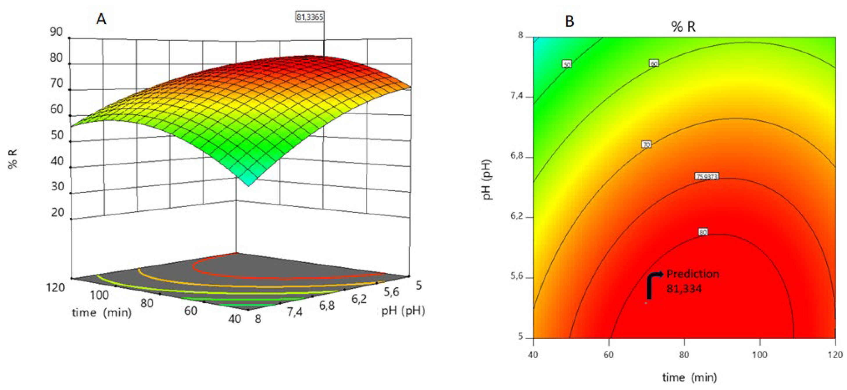
From Equation (18), we can infer that mass (including its interactions with pH and time) is the factor that most affects the response. Mass positively affects the response, while pH does so negatively. This means that if the pH increases, the response decreases. If the pH decreases, the response increases. This is reflected in Figure 9.

Figure 8. A) Dependence of As(V) sorption on pH and time. The response surface was generated using Equation (18); B), the contour surface allows us to visualize the optimal response zone for two independent variables (pH and time) with a prediction of 81.334 of the sorption percentage.

The model optimizes a response of 81.334% sorption. A possible explanation would be the following: As(V) exists in aqueous media as an oxoanion (arsenate) due to its high charge/radius ratio. Speciation depends on the experimental pH. The H₃AsO₄ species has three pKa(Chaudhuri, 2015):

pK_a₁ = 2.19: It corresponds to the first deprotonation.

H₃AsO₄ → H₂AsO₄^- + H⁺

(18)

pK_a₂ = 6.94: Second deprotonation

H₂AsO₄^- → HAsO₄^2- + H⁺

(19)

pK_a₃ = 11.5: Third deprotonation

HAsO₄^2- → AsO₄^3- + H⁺

(20)

The proportion of species present in the reaction medium can be easily estimated from speciation diagrams obtained with the software “Medusa” (Make Equilibrium Diagrams Using Sophisticated Algorithms, Ignasi Puigdomenech, Royal Institute of Technology 100 44 Stockholm, Sweden). Figure 8 shows the speciation diagram and species fraction vs pH (1-12) for As(V) with an initial concentration of 3.54 µM (265 mg/L). Medusa uses the pK_a1-3 values to calculate the species fraction.

Figure 9. Speciation diagrams obtained with the software “Medusa”.

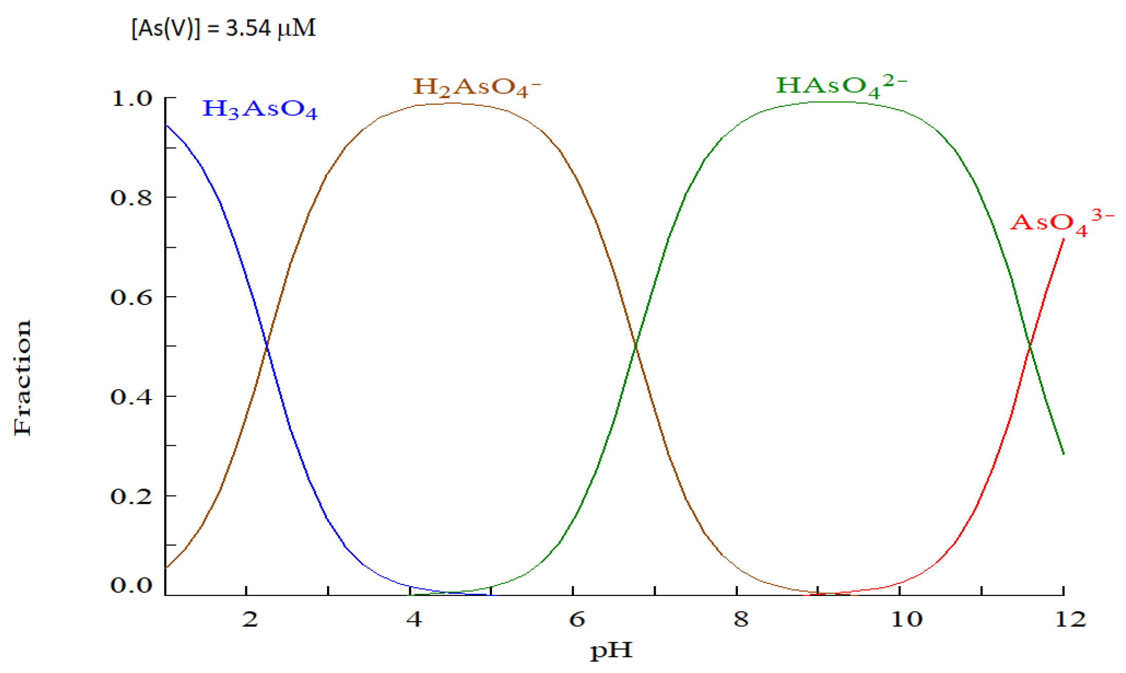
As shown in Figure 3, the surface of the M-Q sorbent is positively charged at pHs lower than 7.8; on the other hand, at pH 5, almost 100% of the As(V) is negatively charged (H₂AsO₄^-). As the pH increases, the species composition of the mixture changes (the H₂AsO₄^- species decreases and the HAsO₄^2- species slightly increases), but the sorbent surface begins to lose positive charge (Figure 3). To conclude, there is a range of favorable pHs for the sorption of As(V) within the acid zone that can be explained by the electrostatic attractions between the species/s of the As(V) oxoanions and the positive surface charge of the -M-Q sorbent surface. Figure 9 A shows this behavior: there is no significant variation in the response at pH 7.4-8. The As(V) sorption increases significantly as pH decreases, at first and then at a lower percentage (pH 5.6-5).

Mass and time also play important roles in the sorption of As(V). According to Equation (18) and Figure 10, a zone of minimum sorption of As(V) is observed (pH = 5 and mass = 0.17 g). As the mass increases, the number of sorption sites also increases. This effect is very evident in the pH range 5.6-5 for high mass. However, sorption is almost independent of pH at very low masses, Figure 10.

The independence of As(V) sorption is also observed when the sorbent is very low. As the mass increases, the response of the system increases, Figure 11

These results were validated in the laboratory in duplicate. The sorption percentage found experimentally for a M-Q mass of 0.43 g, a pH of 5.4, and a contact time of 82 minutes was 75%.

4. Conclusions

This study focuses on the problem of As in drinking water. In particular, it emphasizes the deprived areas near the cities of Rosario and Santa Fe that, for political and/or economic reasons, do not have access to drinking water and must, therefore, resort to consuming groundwater.

This study uses a method for detecting As that does not require much equipment, measurements can be made in the area in question without transporting the samples to large cities, thus avoiding contamination. Detection and quantification using the silver diethyldithiocarbamate technique is accepted(Argentina.gob.ar, 2003) and only requires a few reagents, an extraction hood and a photocolorimeter to read at 530 nm. The methodology is sensitive and reproducible enough to be used in compliance with current regulations.

The synthesis of Q, M, and Q-M spheres was carried out, and XRD characterized them. The syntheses were successful, achieving spheres with a high As sorption capacity and mechanical resistance.

The remediation of As using only Q spheres as sorbent was inappropriate since its optimal value (pH 6.1, mass 0.5 g, and time 120 min) is only 30%. Incorporating M into the Q spheres generates a hybrid sorbent with a sorption capacity of 81% in less time. Beyond the possible mechanisms that may occur for the capture of As, the truth is that the (optimal) response increases by 270% when M is incorporated. It was also demostrated, that Magnetite remains unaltered for, at least 6 months, in aerobic conditions, when incorporated into chitosan spheres, as can be seen by XRD. Another advantage of this hybrid sorbent is the capability of being separated by its magnetic properties, as was probed during this work in our laboratory. We want to highlight the advantages of using a response surface method (multivariate) compared to univariate methods and keeping two factors constant while varying the third leads to obtaining good trends with a relatively large number of experiments: univariate method or one variable at a time (OVAT). Response surface modeling (DOE-SRO: design of experiments-surface response optimization) is more appropriate when the objective is optimization. The advantages of this method are clear: a) SRO provides global information, OVAT only local information; 2) SRO considers interactions between factors, OVAT does not, and 3) The number of experiments required by SRO is lower than OVAT (Montgomery, 2017; Myers et al., 2016).

References

Abanto Pérez, J.A.; Reyes Benites, P.N. (2021). Prototipo de biofiltro con arcilla, cascara de arroz y NaOh para remoción del arsénico del Río Huandoval, Pallasca, Ancash–2021.
Abernathy, C.; Marcus, W.; Chen, C.; Gibb, H.; White, P. (1989). Office of Drinking Water, Office of Research and Development, USEPA. Memorandum to P. Cook, Office of Drinking Water, US EPA and P. Preuss, Office of Regulatory Support and Scientific Management, US EPA.
Argentina.gob.ar. (2003). 540-Limite de Arsenico https://www.argentina.gob.ar/. Retrieved 09-30-2024 from https://www.argentina.gob.ar/normativa/recurso/86181/dto202-2003-61/htm.
Argentino, C.A. (2012). Capítulo XII. Bebidas hídricas, agua y agua gasificada”. Agua potable. Artículo, 982.
Association, A.P.H. (1926). Standard methods for the examination of water and wastewater -3500-Fe IRON (Vol. 6). American Public Health Association. [CrossRef]
Bardach, A.E.; Ciapponi, A.; Soto, N.; Chaparro, M.R.; Calderon, M.; Briatore, A.; Cadoppi, N.; Tassara, R.; Litter, M.I. Epidemiology of chronic disease related to arsenic in Argentina: A systematic review. Sci. Total. Environ. 2015, 538, 802–816. [Google Scholar] [CrossRef] [PubMed]
Batistelli, M.; Bultri, J.; Trespalacios, M.H.; Mangiameli, M.F.; Gribaudo, L.; Bellú, S.; Frascaroli, M.I.; González, J.C. Elimination of Arsenic Using Sorbents Derived from Chitosan and Iron Oxides, Applying Factorial Designs. Inorganics 2023, 11, 428. [Google Scholar] [CrossRef]
Benítez, E.M.L.; Verdecia, G.M.; Castell, M.A.P. Escasez y contaminación del agua, realidades del siglo XXI. Revista 16 de abril 2021, 60, 854. [Google Scholar]
Chaudhuri, P.P. (2015). Groundwater arsenic remediation: treatment technology and scale UP. Butterworth-Heinemann.
Corey, G.; Tomasini, R.; Pagura, J. (2005). Estudio epidemiológico de la exposición al arsénico a través del consumo de agua. Provincia de Santa Fe, República Argentina. In: Santa Fe: Gobierno de Santa Fe.
Cuizano, N.A.; Llanos, B.P.; Navarro, A.E. Aplicaciones ambientales de la adsorción mediante biopolímeros naturales: Parte 1-Compuestos fenólicos. Revista de la Sociedad Química del Perú 2009, 75, 488–494. [Google Scholar]
Edition, F. Guidelines for drinking-water quality. WHO chronicle 2011, 38, 104–108. [Google Scholar]
ENRRES, r. (2016).
García, J.; Sotomayor, N.J.G.; Becerra, J.S.C. (2023). Residuos orgánicos agroindustriales empleados para la remoción de arsénico en soluciones acuosas. Encuentro Internacional de Educación en Ingeniería.
Litter, M. (2018). Arsénico en agua.
Loomis, D.; Guha, N.; Hall, A.L.; Straif, K. Identifying occupational carcinogens: an update from the IARC Monographs. Occup. Environ. Med. 2018, 75, 593–603. [Google Scholar] [CrossRef] [PubMed]
Marchetti, M.D.; Tomac, A.; Perez, S. Perfil de riesgo para la inocuidad de alimentos: presencia de arsénico en Argentina. Revista Argentina de Salud Pública 2021, 13, 191–200. [Google Scholar]
Martínez-Cabanas, M. (2017). Desarrollo de materiales híbridos para la eliminación de arsénico de medios acuosos Universidade da Coruña].
Molinari, A.; Bos, R.; Latorre, C.; Bedoya, C.; del Rosario Navia, M. (2021). Los reguladores y la implementación de los derechos humanos al agua y saneamiento en América Latina y el Caribe.
Montgomery, D.C. Design and analysis of experiments. John wiley & sons.
Moreira, V.; Lebron, Y.; Santos, L.; de Paula, E.C.; Amaral, M. Arsenic contamination, effects and remediation techniques: A special look onto membrane separation processes. Process. Saf. Environ. Prot. 2020, 148, 604–623. [Google Scholar] [CrossRef]
Mular, A.; Roberts, R. A simplified method to determine isoelectric points of oxides. Canadian Mining and Metallurgical Bulletin 1966, 59, 1329. [Google Scholar]
Myers, R.H.; Montgomery, D.C.; Anderson-Cook, C.M. (2016). Response surface methodology: process and product optimization using designed experiments. John Wiley & Sons.
Nawrocka, A.; Durkalec, M.; Michalski, M.; Posyniak, A. Simple and reliable determination of total arsenic and its species in seafood by ICP-MS and HPLC-ICP-MS. Food Chem. 2022, 379, 132045. [Google Scholar] [CrossRef] [PubMed]
O’reilly, J.; Watts, M.J.; Shaw, R.A.; Marcilla, A.L.; Ward, N.I. Arsenic contamination of natural waters in San Juan and La Pampa, Argentina. Environ. Geochem. Heal. 2010, 32, 491–515. [Google Scholar] [CrossRef] [PubMed]
Paredes Ramirez, E.O.; Segura Acosta, L.M. (2021). Estudio de la remoción de metales pesados en aguas contaminadas de ríos utilizando carbón activado vegetal.
Reventós, M.M.; Rius, J.; Amigó, J.M. Mineralogy and geology: The role of crystallography since the discovery of X-ray diffraction in 1912. Revista de la Sociedad Geológica de España 2012, 25, 133–143. [Google Scholar]
Sardar, M.; Manna, M.; Maharana, M.; Sen, S. (2021). Remediation of dyes from industrial wastewater using low-cost adsorbents. Green adsorbents to remove metals, dyes and boron from polluted water, 377-403.
Srinivasan, S.; Chelliah, P.; Srinivasan, V.; Babu, A.; Subramani, K. Chitosan and Reinforced Chitosan films for the Removal of Cr(VI) Heavy Metal from Synthetic Aqueous Solution. Orient. J. Chem. 2016, 32, 671–680. [Google Scholar] [CrossRef]
Silva Lizama, P.B. (2023). Preparación y evaluación de bentonita intercalado con óxido de hierro para la remoción de arsénico en aguas contaminadas.
Singh, R.; Singh, S.; Parihar, P.; Singh, V.P.; Prasad, S.M. Arsenic contamination, consequences and remediation techniques: A review. Ecotoxicol. Environ. Saf. 2015, 112, 247–270. [Google Scholar] [CrossRef] [PubMed]
UNICEF. (2018). Arsenic primer: guidance on the investigation & mitigation of arsenic contamination. New York: UNICEF Water, Sanitation and Hygiene Section and WHO Water, Sanitation and Hygiene and Health Unit, United Nations Children’s Fund (UNICEF).
Waseda, Y.; Matsubara, E.; Shinoda, K. (2011). X-ray diffraction crystallography: introduction, examples and solved problems. Springer Science & Business Media.
Wastewater S-f t E o W, a. (2017) 3500-As, B. Silver Diethyldithiocarbamate Method. [CrossRef]

Figure 1. Representation of the interaction of X-rays on the planes of a sample, according to Bragg's Law.

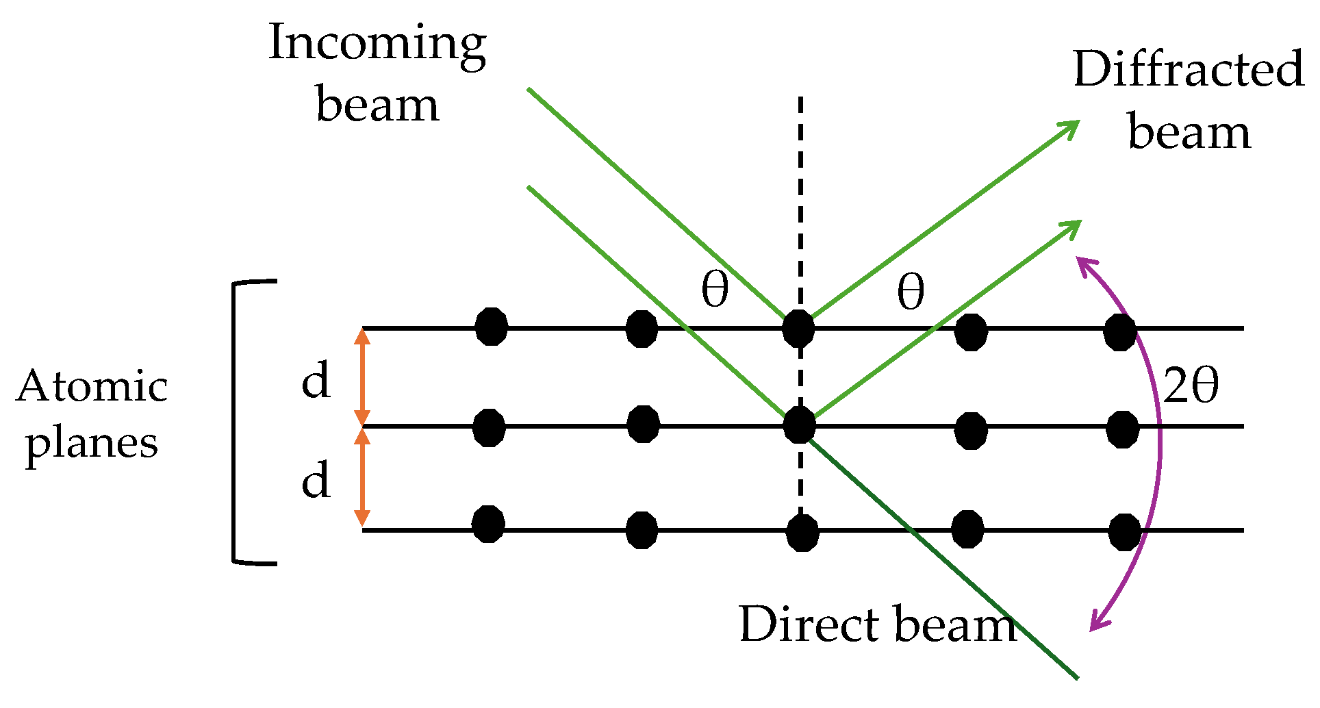
Figure 2. Experimental equipment used for the determination of As.

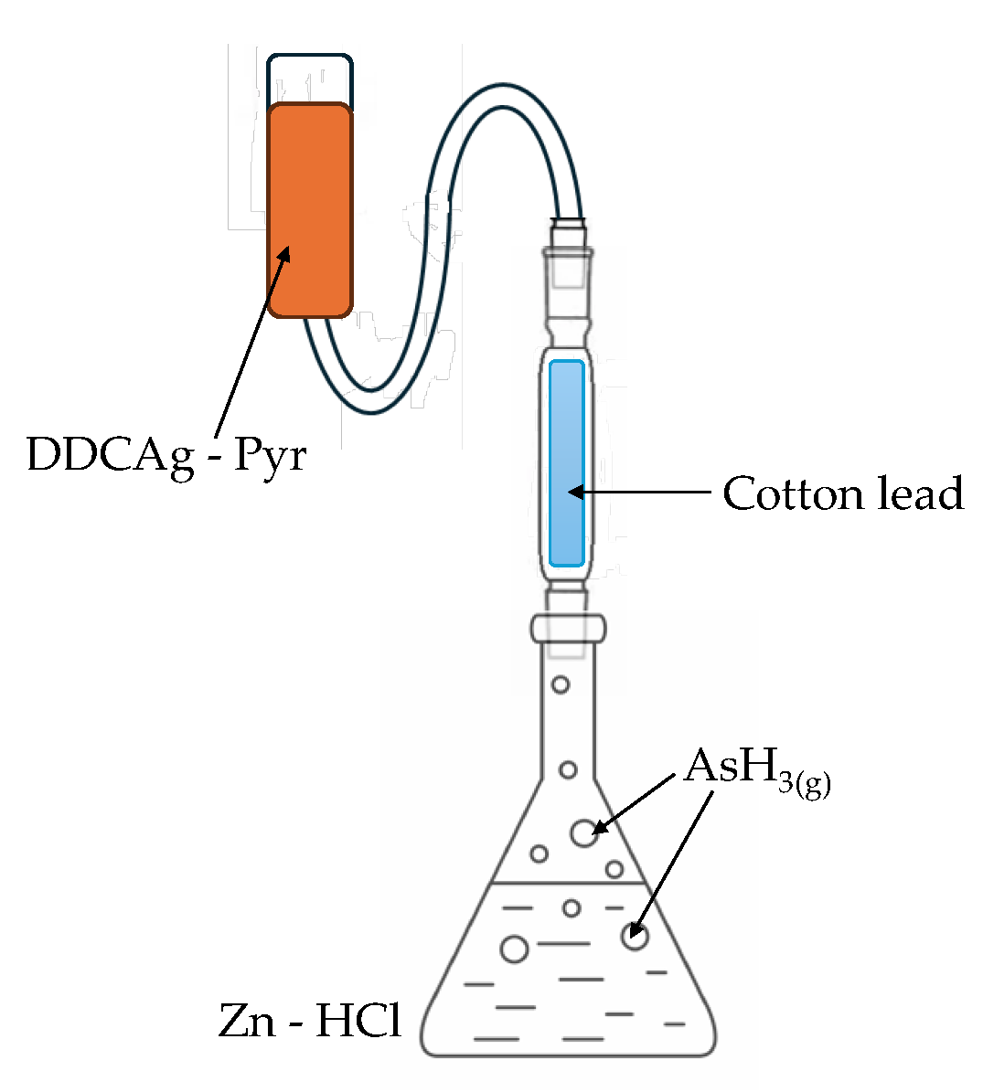
Figure 3. Graphical determination of sorbent pH_zc for Q and Q-M sorbents.

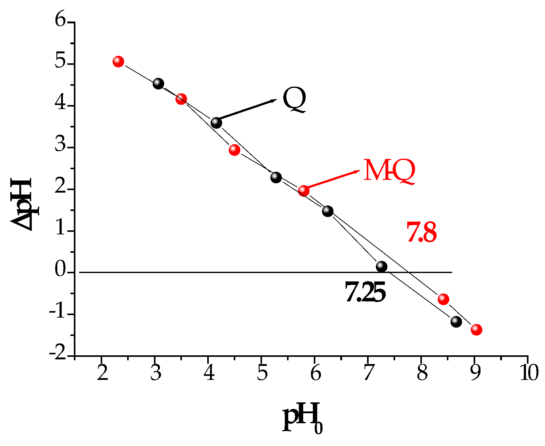
Figure 4. RDX diffractograms of Q, M, M-Q, M-Q-As, and M-Q-As-T (Waseda et al., 2011).

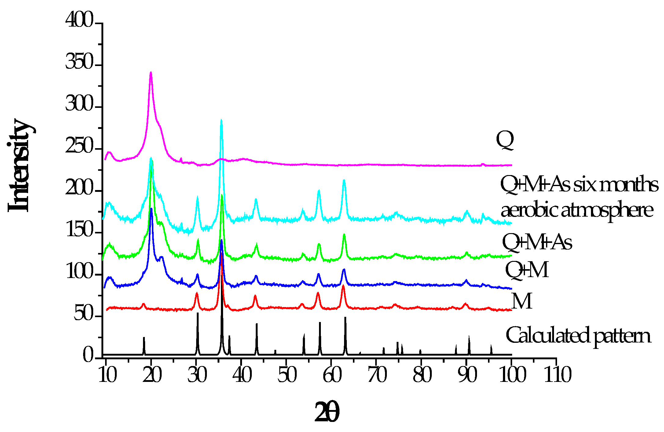
Figure 5. Calibration curve for As(V) dosage by the DDCAg method.

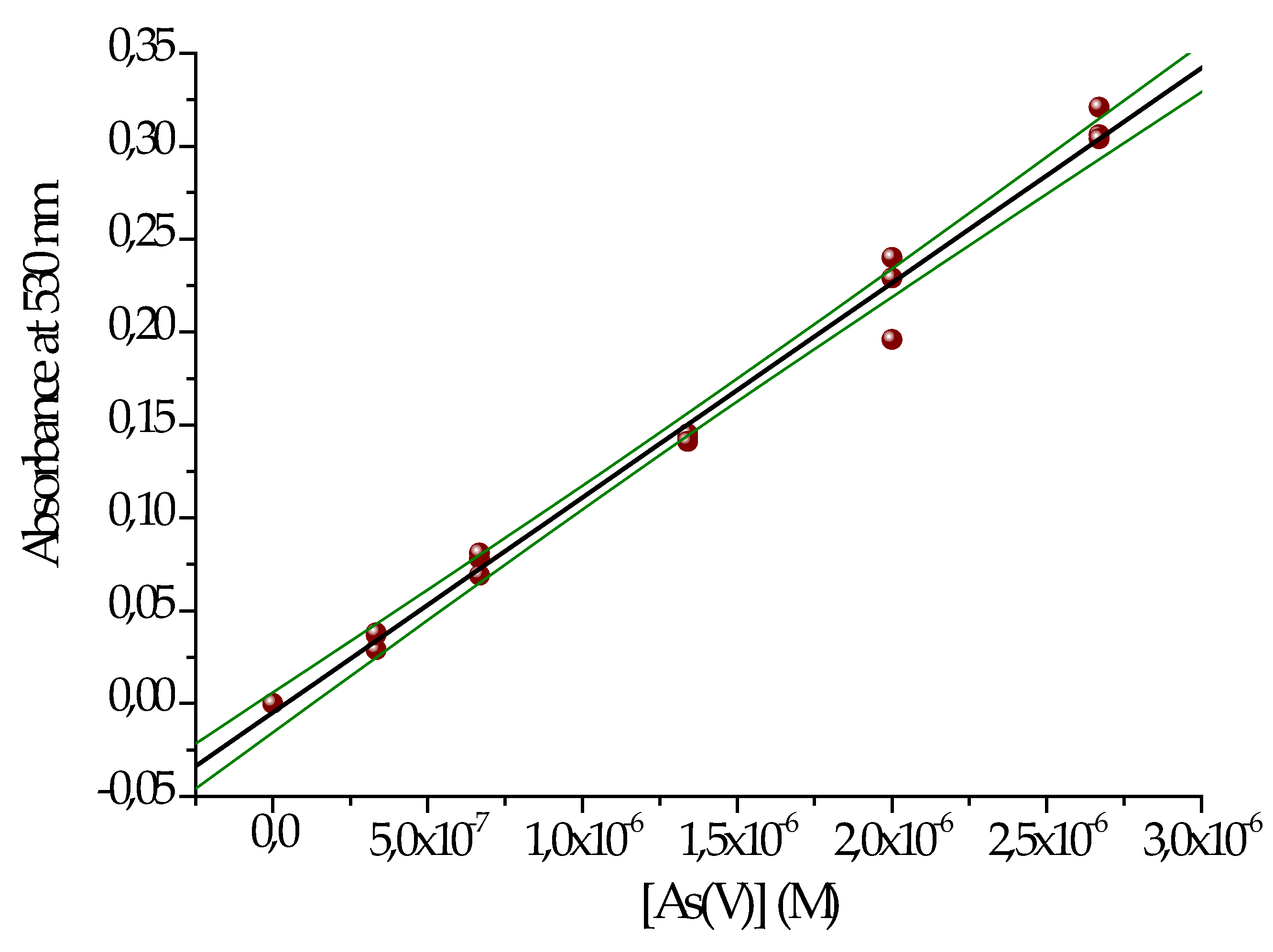
Figure 6. Predicted vs experimental plot for As sorption with M-Q and Q.

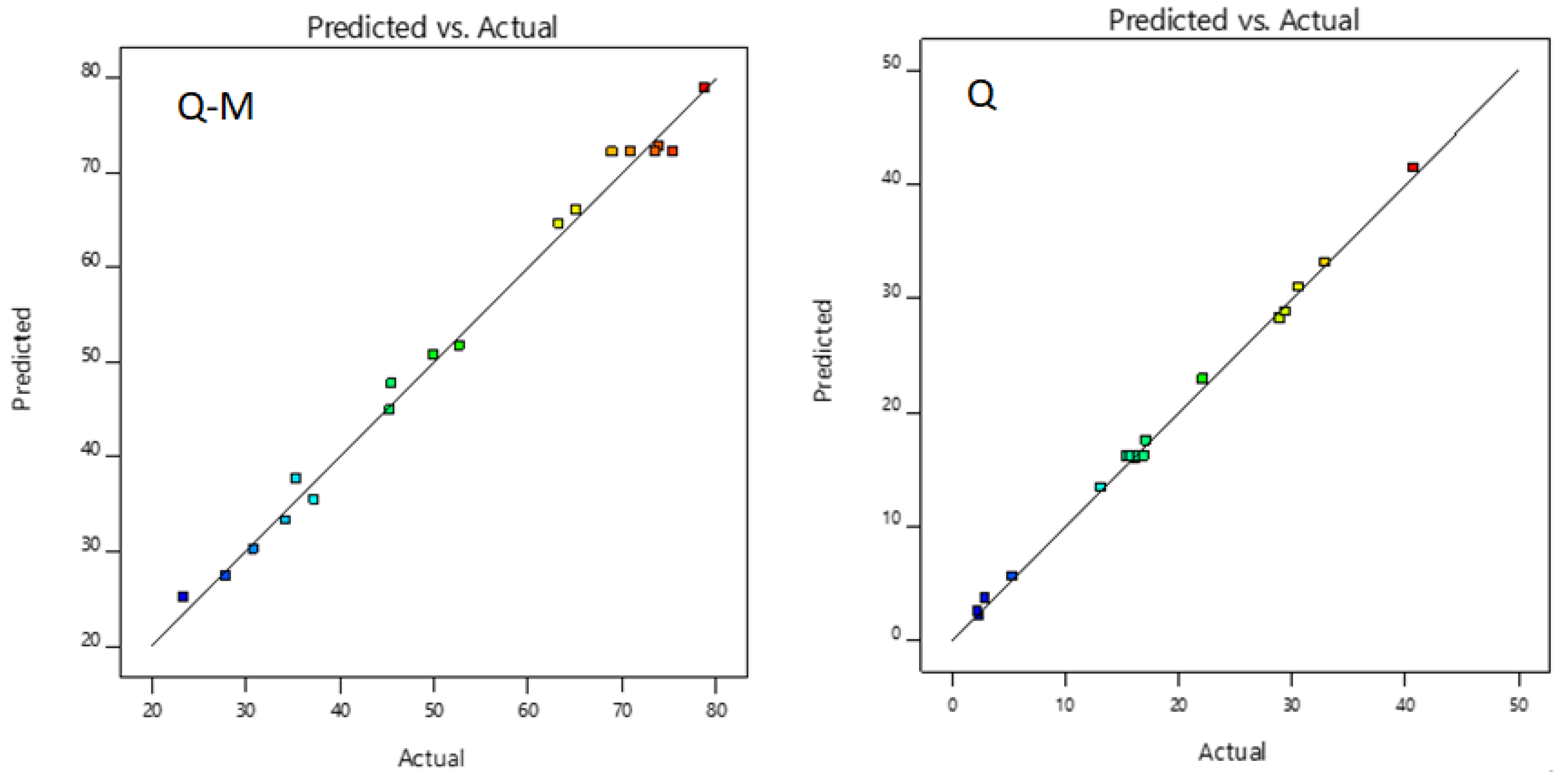
Figure 7. Residual vs. Predicted plot for As sorption with -M-Q and Q.

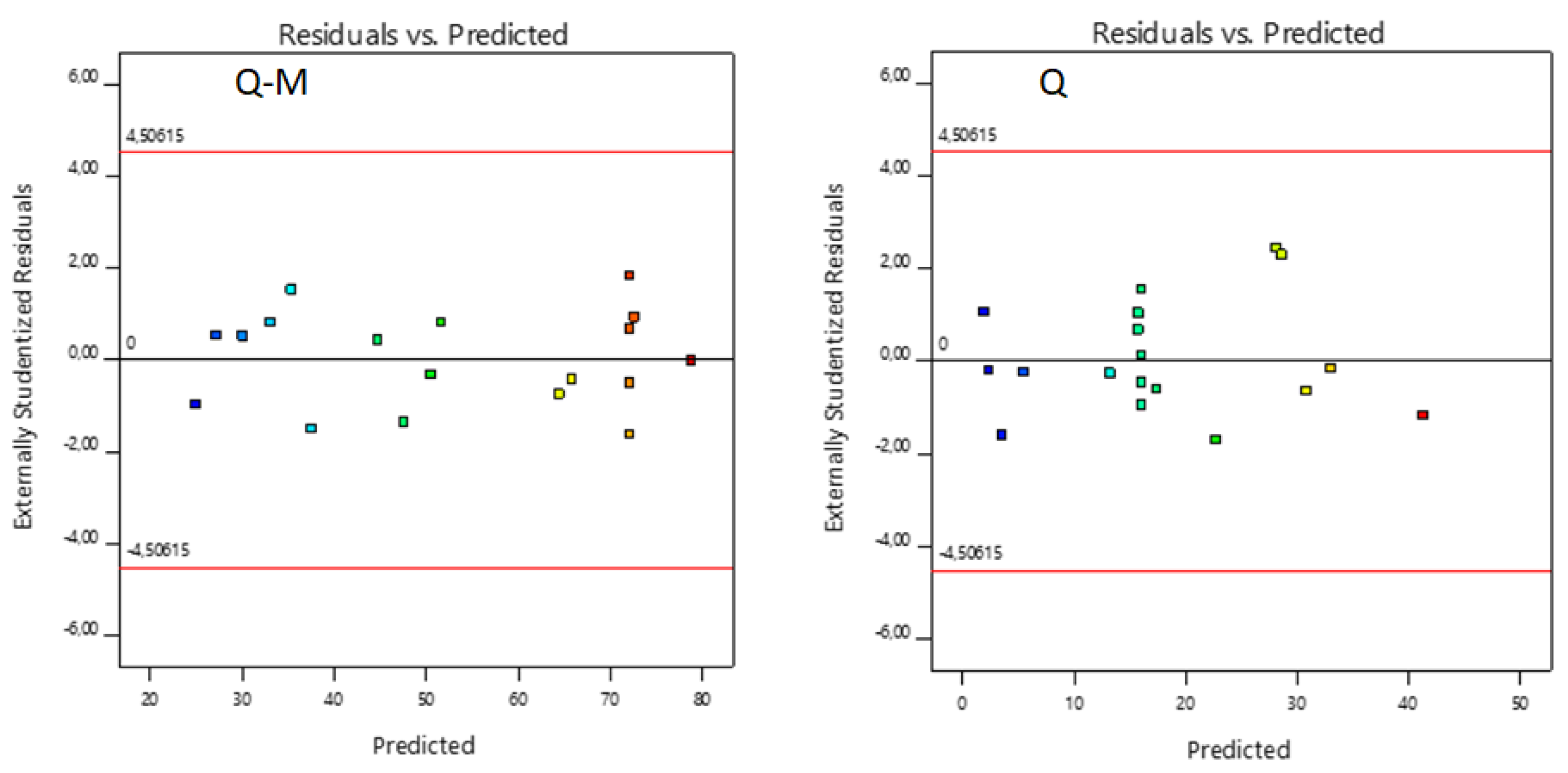
Figure 10. A) Dependence of As(V) sorption on mass and pH; B) corresponding contour surface.

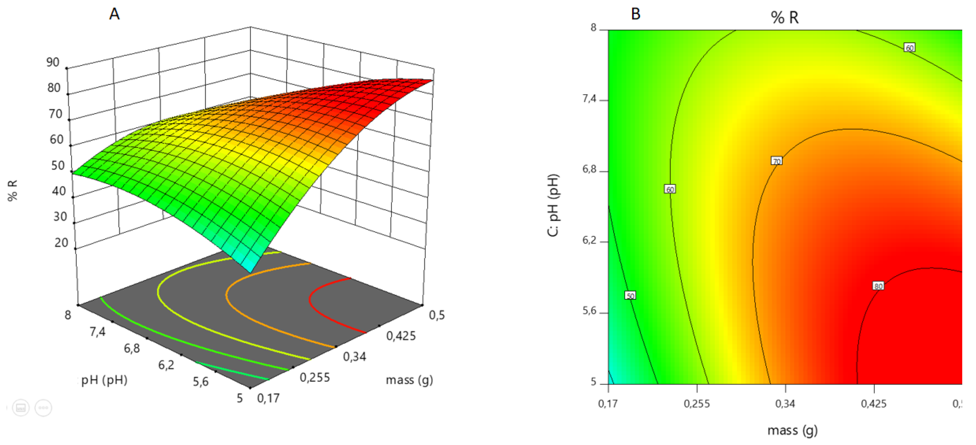
Figure 11. A) Dependence of As(V) sorption on mass and time; B) corresponding contour surface.

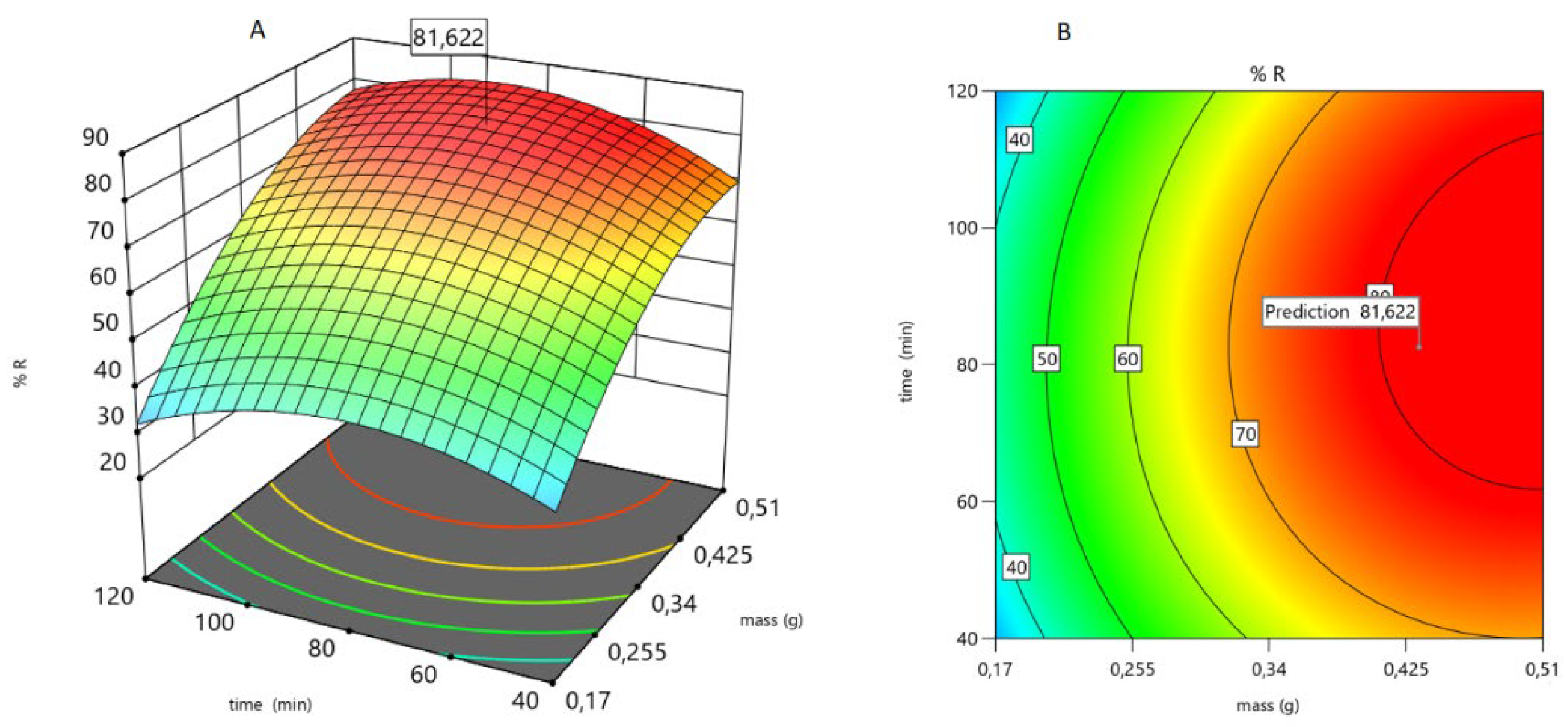
Table 1. Instrumental setup for XRD tests.

Instrumental setup/Methodology used	Bragg Value/Concept
Geometry - Setup	Bragg Brentano θ-θ
2θ angular range	5 - 100°
Time per step	1 s
Step size	0,04 °
Voltage	30 kV
Current	10
Divergence slot (primary)	mA
2θ angular range	1 mm

Table 2. Protocol used for the determination of As(V) by the DDCAg method, calibration curve: quantities and order of reagents addition.

Conical flask, final volume, 50 mL, As(V), M	0	3.34 10^-07		6.68 10^-07	1.34 10^-06	2.00 10^-06	2.67 10^-06
Distilled water, mL	50		-	-	-	-	-
HCl 37%W/W; density 1.17 g/cm³, mL	5		5	5	5	5	5
KI 0.1 M, mL	2		2	2	2	2	2
SnCl₂ 0.15 M, mL	0.5		0.5	0.5	0.5	0.5	0.5
15 minutes. Grease the ground joints and place the filter soaked in lead acetate solution.
Activated Zn Shots (tablespoons), g	3.1		3.1	3.1	3.1	3.1	3.1
Cover immediately and place in the reaction cup.
(DDCAg) 0.5% W/V dissolved in Pyr, mL	4		4	4	4	4	4
Check for bubbles in the reaction cup. Wait 30-45 minutes. Transfer the liquid from the cup to the reading cuvette, 1 cm optic pass. Read in a photometer at 530 nm, bringing it to zero with distilled water.

Table 3. A. Coded levels used in the CCD for Q.

Factors	Symbols	Minimum	Maximum	Code Low	Code High	Mean
Mass (g)	A	0.0680	0.7840	-1 ↔ 0.20	+1 ↔ 0.50	0.4260
Time (min)	B	13.00	147.00	-1 ↔ 40.00	+1 ↔ 120.00	80.00
pH	C	4.00	9.00	-1 ↔ 5.00	+1 ↔ 8.00	6.50

Table 3. B. Coded levels used in the CCD for Q-M.

Factors	Symbols	Minimum	Maximum	Code Low	Code High	Mean
Mass (g)	A	0.0600	0.6300	-1 ↔ 0.17	+1 ↔ 0.51	0.3406
Time (min)	B	13.00	147.00	-1 ↔ 40.00	+1 ↔ 120.00	80.00
pH	C	4.00	9.00	-1 ↔ 5.00	+1 ↔ 8.00	6.50

Table 4. Groundwater characterization.

Analyte	Sample (mg/L)	Limit CCA (mg/L)	Method
pH	7.8¹	6.5 – 8.5¹	Potentiometric
Total dissolved solids	11392.0	300-6000	Gravimetric
Nitrates	16.0	45.0	Selective electrode
Nitrites	0.003	0.10	Colorimetric
Fluoruro	2.0	1.5	Colorimetric
ammonia	ND	0.2	Colorimetric
Sulfates	240.7	400.0	Turbidimétrico
Phosphates	2.2 x 10^-3	1.5	Colorimetric
Silicates	41.6	10.0 – 30.0	Colorimetric
Conductivity	12.1²	***	Conductimetric
Hardness	1125³	51³	Titrimeric
As(total)	0.015	0.01	Colorimetric

¹pH units; ²µS/cm; *** Until 2012, the current regulations of Santa Fe did not establish limits; ³ expressed as mg/L of CaCO₃; ND: not detected; CAA (Argentine Food Code, for the acronym in Spanish).

Table 5. As(V)-DDCAg calibration curve parameters.

Parameters	Formula	Values	Units
Slope (A)	Slope ± S_A	116.000 ± 3,000 1.54 ± 0.0420	M^-1 Mg/L
Intercept (B)	Intercept ± S_B	-0.005 ± 0.005	M^-1
Determination coefficient R²	R² of calibration curve	0.990
Relative standard deviation of the slope of the calibration curve	S_A*100/slope	2.7	%
Limit of Detection	LD = 3.3*Sb/slope	1.42x10^-7 0.0110	M mg/L
Limit of Quantification	LQ = 10*S_B/slope	4.32 x 10^-7 0.032	M mg/L
Lineal range	F_exp = 1.02 F_14,11 = 2.85	4.32x10^-7 2.67x10^-6 0.0323- 0.200	M mg/L
Uncertainty (SC)	$S C = \frac{S y / x}{S l o p e} \sqrt{\frac{1}{m}}$	0.0042	mg/L

Table 6. Values for each factor generated using CCD, for the M-Q and Q sorbents.

M-Q Spheres				Q Spheres
Mass(A)	Contact time(B)	pH(C)	% R	Mass(A)	Contact Time(B)	pH(C)	% R
g	min	pH	%	g	min	pH	%
0.34	80	6.5	71.02	0.426	80	4.0	5.40
0.06	80	6.5	23.59	0.426	80	6.5	15.50
0.63	80	6.5	63.40	0.213	120	8.0	17.18
0.34	80	9.0	45.66	0.426	80	6.5	15.80
0.51	120	5.0	78.82	0.426	13	6.5	16.15
0.51	40	8.0	34.34	0.784	80	6.5	33.00
0.17	120	5.5	28.00	0.639	40	8.0	22.20
0.34	80	6.5	75.47	0.213	120	5.0	29.00
0.34	80	6.5	69.06	0.068	80	6.5	13.20
0.34	80	6.5	73.58	0.639	40	5.0	16.26
0.17	40	8.0	37.36	0.426	80	9.0	2.30
0.34	13	6.5	35.47	0.213	40	5.0	3.00
0.51	40	5.0	73.96	0.426	80	6.5	16.18
0.34	147	6.5	50.08	0.639	120	8.0	29.50
0.34	80	4.0	65.20	0.639	120	5.0	30.61
0.51	120	8.0	52.83	0.426	80	6.5	17.00
0.17	40	5.0	30.91	0.426	147	6.5	40.83
0.17	120	8.0	45.41	0.213	40	8.8	2.47

Table 7. ANOVA for Quadratic model, response: %R.

Surce	Sum of Squeres	df	Mean Square	F Value	p-value Prob>F	Q-M	Sum of Squeres	df	Mean Square	F Value	p-value Prob>F	Q
Model	5826,1	9	647.3	112.57	< 0.0001	S	2088.7	9	232.1	438.12	< 0.0001	S
A-mass	2074.6	1	2074.6	360.8	< 0.0001	S	146.8	1	146.8	277.13	< 0.0001	S
B-time	206.1	1	206.1	35.8	0.0003	S	802.4	1	802.4	1514.72	< 0.0001	S
C-pH	407.4	1	407.4	70.8	< 0.0001	S	32.3	1	32.3	60.99	< 0.0001	S
AB	41.4	1	41.4	7.2	0.0277	S	45.4	1	45.4	85.72	< 0.0001	S
AC	1000.6	1	1000.6	174.0	< 0.0001	S	36.9	1	37.0	69.65	< 0.0001	S
BC	75.6	1	75.6	13.1	0.0067	S	42.0	1	42.0	79.37	< 0.0001	S
A2	1218.1	1	1218.1	211.8	< 0.0001	S	79.9	1	80.0	150.88	< 0.0001	S
B2	1250.4	1	1250.4	217.4	< 0.0001	S	248.0	1	248.0	468.12	< 0.0001	S
C2	377.1	1	377.1	65.6	< 0.0001	S	235.43	1	235.4	444.43	< 0.0001	S
Residual	46.0	8	5.75				4.24	8	0.53
Lack of Fit	22.2	5	4.44	0.557	0.7345	NS	2.97	5	0.60	1.41	0.4132	NS
Pure Error	23.8	3	7.94				1.26	3	0.42
Cor Total	5872.1	17					2092.97	17

S: significant; NS: not significant.

Table 8. Fit Statistics.

M-Q				Q
Std. Dev.	2.40	R²	0.9922	Std. Dev.	0.7278	R²	0.9980
Mean	53.01	Adjusted R²	0.9834	Mean	18.09	Adjusted R²	0.9957
C.V. %	4.52	Predicted R²	0.9642	C.V. %	4.02	Predicted R²	0.9864
		Adeq Precision	30.0881			Adeq Precision	72.4948

Table 9. Coefficients in Terms of Coded Factors.

M-Q	Estimate		Error	Low	High	VIF
Intercept	72.14	1	1.20	69.39	74.90
A-masa	12.35	1	0.6501	10.85	13.85	1.00
B-tiempo	3.89	1	0.6500	2.39	5.39	1.0000
C-pH	-5.48	1	0.6513	-6.98	-3.98	1.0000
AB	2.28	1	0.8478	0.3211	4.23	1.0000
AC	-11.18	1	0.8478	-13.14	-9.23	1.0000
BC	3.07	1	0.8478	1.12	5.03	1.0000
A²	-9.85	1	0.6765	-11.41	-8.29	1.08
B²	-9.99	1	0.6778	-11.56	-8.43	1.07
C²	-5.53	1	0.6834	-7.11	-3.96	1.07

Disclaimer/Publisher’s Note: The statements, opinions and data contained in all publications are solely those of the individual author(s) and contributor(s) and not of MDPI and/or the editor(s). MDPI and/or the editor(s) disclaim responsibility for any injury to people or property resulting from any ideas, methods, instructions or products referred to in the content.

© 2024 by the authors. Licensee MDPI, Basel, Switzerland. This article is an open access article distributed under the terms and conditions of the Creative Commons Attribution (CC BY) license (http://creativecommons.org/licenses/by/4.0/).

Copyright: This open access article is published under a Creative Commons CC BY 4.0 license, which permit the free download, distribution, and reuse, provided that the author and preprint are cited in any reuse.

MDPI Initiatives

Important Links

Choose an area of interest and we will send you notifications of new preprints at your preferred frequency.

Disclaimer