
Submitted:
02 October 2024
Posted:
03 October 2024
You are already at the latest version
Abstract
The abstract should be an objective representation of the article and it must not contain results that are not presented and substantiated in the main text and should not exaggerate the main conclusions.
Keywords:
ecosystems
; mapping
; land‐cover
; remote sensing
; sentinel‐2
; machine learning
; image classification
; vegetation
1. Introduction
Spatial depictions of land-cover are integral to effective ecological and environmental management. Additionally, the thematic resolution of land-cover and vegetation maps contributes significantly to the effective development of policies and land management decisions based on spatial data. The importance of classifying and mapping vegetation has been widely acknowledged given the essential role it plays in wildlife habitat, biodiversity, ecosystem services and climate regulation [1,2]. Other considerations, such as the implementation of ecosystem restoration or preservation programs, also require that vegetation be mapped throughout time to serve as reference points for future comparisons.
Spatial ecosystems classifications can be broadly lumped into one of two categories: 1) geophysical-based classifications derived mainly from geophysical settings and abiotic factors, and 2) integrated classifications that combine remotely sensed land cover data with abiotic and geophysical factors. While ecological mapping efforts based on stratifications of various geophysical data layers provide a good foundation for ecological assessments, they are conceptual in nature and depict reference states rather than the actual location of different vegetation or ecological types. Rather, they serve more as a guide to potential ecological states in various locations [3,4].
Some past efforts have been made to link remote sensing and ancillary modeling approaches to produce detailed ecosystem and vegetation maps. Jung et al. (2020) used global 100-meter resolution land-cover along with various rulesets to generate a 47-class global map of terrestrial habitat types [5]. In another study, a 250-meter resolution global dataset depicting 431 world terrestrial ecosystems was created using a combination of climate regions, landform models and land-cover, and biogeographic realm [6]. However, while such global datasets serve as useful tools for national or multi-state planning efforts, they do not offer the precision that is often required for practitioners at county, state, or provincial scales to meet more localized objectives, either in terms of spatial or thematic resolution [7]. There have been some notable attempts to incorporate remotely sensed data to produce improved resolution ecosystem and vegetation maps. For instance, the Gap Analysis Project (GAP) and LANDFIRE Existing Vegetation Type (EVT) datasets provide terrestrial ecological systems classifications for the entire United States, driven by classifications of 30-meter Landsat satellite imagery combined with bio- and geophysical setting data [8,9]. Yet these efforts are conduct nationally, and their accuracy is generally low when compared with field-based data and other land-cover datasets [10,11,12]. In addition, their ability to realistically circumscribe vegetative features using a 900 m2 grid cell resolution is limited [13,14]. However, the detection and realistic spatial depiction of landscape features, particularly vegetation, is of great importance for a wide range of environmental and conservation management concerns. Specifically, the spatial and thematic resolution of vegetation data has implications for water estimations in hydrological models, fire intensity and extent in predictive wildfire models, sustainability planning, and wildlife habitat management [15,16,17]. Furthermore, the satellite spatial resolution underlying a given ecological systems classification is critical since large amounts of tree and shrub cover can go completely undetected at coarser scales [18]. This is of particular importance in landscapes such as mixed woodland-grassland ecosystems, such as savannas, or transitional zones where forest and herbaceous types intermix [19,20].
Given that widely available land-cover and vegetation datasets are generally lacking in either thematic resolution or spatial resolution, there is ongoing need to integrate modeling techniques and ancillary data with traditional satellite image classifications to produce more detailed ecosystem maps over large areas. Results from such mapping efforts can serve as effective decision tools and model inputs for local and regional conservation planners and environmental modelers. To address this, we present a comprehensive approach using satellite imagery, field training data, machine learning, image segmentation, and ancillary modeling approaches to develop high-resolution ecological system type maps statewide for Arkansas, USA (Figure 1). The overarching goal of this work was to address the shortcomings described for other ecological and vegetation mapping efforts, and to provide a framework for future mapping efforts to facilitate improved natural resource management, wildlife conservation, and environmental modeling.
2. Materials and Methods
2.1. Study Area
The study area included the entire state of Arkansas, which is situated in the Southeastern United States. The state resides at the confluence of several significant ecoregions, including the Ozark Highlands, Arkansas Valley, South Central Plains, Ouachita and Boston Mountains, Mississippi Alluvial Plain, and Mississippi Valley Loess Plains [21]. These regions represent diverse land-cover and ecosystem types, ranging from rugged mountainous areas in the central-western and northwestern portions of the state to low-lying areas along the Mississippi River in the east.
We identified the prevailing ecological systems for the entire state (Figure 2) using a combination of two potential natural vegetation datasets. The first of these was developed by grouping SSURGO [22] map unit polygons to create soil eco-groups based on shared characteristics and classifying the grouped map units based on NatureServe Terrestrial Ecological Classifications [23]. The grouping process was facilitated by the NRCS ecological site descriptions, which are attached to SSURGO soil components [24,25]. We assigned soil eco-group using expert opinion where the NRCS had not yet assigned ecological sites to soil components in some eastern portions of the state. The second dataset used covered the Mississippi Alluvial Valley region, and depicted potential natural vegetation based on basin-level functional wetland assessments, which were drafted from a merging of surface geology, soils maps, and flooding maps [26,27].
2.2. Training Data Generation & Classification of Sentinel-2 Imagery
Training data for the landcover classification were generated primarily from photointerpretation of high-resolution aerial imagery using a random grid of points within each of three mapping zones covering the state (Figure 3). A total of 12 land cover class targets were identified (Table 1). Field collected plots were not directly used as samples for the landcover classification but were used to aid in photo survey sample interpretation, particularly for distinguishing between eastern redcedar versus pine landcover classes. The total number of samples collected within each of the primary mapping zones ranged from 2500 to 3000.
Remotely sensed data from the Copernicus Sentinel-2 earth observation mission [28] was surveyed in order to identify cloud-free imagery for the entire state of Arkansas. The Sentinel-2 mission consists of a constellation of two satellites (Sentinel-2A and Sentinel-2B), each carrying a Multispectral Instrument (MSI) designed to measure the reflected radiance of Earth in 13 spectral bands. Of interest for this project were: visible and near-infrared bands at 10 meters, and red edge and SWIR bands at 20 meters [29]. Imagery for the study region was selected based on a combination of recency and clarity (i.e., the absence of clouds). Given the extent of the study area, it was necessary to assess and compile imagery for multiple zones (Zone 1, Zone 2, and Zone 3), each corresponding to Sentinel-2 orbits (Figure 3). Multiple imagery dates from 2020—2021 (early growing season, late growing season, leaf-off) were selected for each of the three primary Sentinel-2A/2B orbits/zones passing over the state of Arkansas. After selecting the imagery, Sentinel-2 Level-2A (atmospherically corrected surface reflectance) image tiles were loaded into the Google Earth Engine (GEE) cloud computing platform for analysis. A subset of the available spectral bands for each image date was used. The selected bands included: band 2 (blue), band 3 (green), band 4 (red), bands 5, 6, and 7 (red-edge 1, 2, and 3), band 8 (near-infrared 1), band 8a (near-infrared 2), band 11 (shortwave infrared 1), and band 12 (shortwave infrared 2). The spatial resolution of bands 2 through 8 was 10 meters. Bands 5, 6, 7, 8A, 11 and 12, whose native resolutions are 20 meters, were resampled to 10 meters. In addition to the spectral bands, the Normalized Difference Vegetation Index (NDVI) [30], Enhanced Vegetation Index-2 (EVI2) [31], and the Normalized Difference Water Index (NDWI) [31], were calculated. Since it was designed as a complementary index to capture changes in canopy water content, the NDWI was calculated only for the late leaf-on dates, as they reflected peak vegetation/canopy growth.
The photo interpreted training samples were then used to train a RandomForest [32] classifier. Parameter values for all model runs were set as follows: number of trees = 1500, and number of variables randomly sampled at each split = 6. In order to optimize the landcover classification results, multiple model runs were executed for each zone based on iteratively modified training data. The final RandomForest model for each of the zones was then applied to their respective image stack in order to generate a prediction raster, one for each zone. Finally, additional samples for pine woodland and forest and eastern redcedar woodland and shrubland were obtained for zones 1 and 2. These samples were later used to modify the landcover assignment for all pixels that were initially classified as pine or eastern redcedar in earlier iterations of the classification. The final raster zones were merged to produce a single statewide land-cover dataset to be used in the subsequent modeling process.
2.3. Image Classification Refinements
Several raster-based mask layers were developed in order to further refine the RandomForest landcover predictions. These included: (1) an urban area mask, outside of which pixels classified as urban landcover were recoded to barren, (2) a crop area mask, outside of which pixels classified as crop were coded to herbaceous vegetation, (3) a water mask, within which pixels classified as urban and other types of land cover were converted to water to alleviate the issue of errant pixels situated within water bodies, and (4) a pine landscape mask, which was used to model pine plantation types.
2.3.1. Urban Masks
An urban area correction mask was created from the Microsoft computer generated building footprints for the United States database [33], as well as the National Land Cover Database (NLCD) [34] urban landcover classes. Building footprints converted into a 10-meter raster layer and were expanded by five pixels. The NLCD urban classes (classes 21 through 24) were re-sampled from 30-meter to 10-meter pixels and also expanded by five pixels (i.e., 50 meters). This mask was used to reclassify all pixels outside the mask that were originally classified as Developed Impervious Cover or Developed Mixed Intensity Urban to Barren in order to minimize the amount of spurious urban pixels across the landscape.
2.3.2. Crop and Water Masks
A crop mask was produced from the annual Cropland Data Layer (CDL) [35], where a given pixel was included if it was classified as crop in at least one of the five years from 2017 through 2021. Row Crop landcover outside of the mask was reclassed to Herbaceous landcover to minimize the amount of errantly classified Row Crop cover. A water mask was produced using the Copernicus Programme Global Surface Water dataset (GSW) [36]. Multiple 30-meter surface water occurrence tiles corresponding to the statewide extent of Arkansas were mosaicked and resampled to 10-m pixels. Areas where water occurred for at least 25 years during the period from 1984 to 2021 were then selected, and the result was shrunk by two pixels. This mask was then used to reclassify errant landcover pixels residing within areas of water.
2.4. Modeling Ecological Systems
Modeling of the ecological mapping targets was a complicated, multiple-step process. This process is outlined in detail below.
2.4.1. Generation of Image Objects
Trimble eCognition software was used to generate image objects. Two dates of Sentinel-2 data were used for image object generation: late season leaf-on and leaf-off. Data stacks included the red, green, blue, and near infrared (RGBN) bands. The red and blue bands were assigned a weight of 1 and the near infrared and green bands were weighted 2. The scale parameter was 40, shape 0.1, and compactness 0.7. Objects were developed by 100 km square tile. This process produced a vector feature class containing polygons that represented relatively homogeneous units (relative to the Sentinel-2 datasets). The average size of the generated polygons was approximately 0.3 hectares. Since this represents the same area as 30, 10 m Sentinel-2 pixels, any ‘salt and pepper’ effects produced during landcover classification from landcover assigned to 10-meter pixels was substantially smoothed.
2.4.2. Attribution of Landcover and Geophysical Setting to Image Objects
Landcover class and geophysical setting information were assigned to each image object. Percent slope and solar radiation were calculated from a 10 m digital elevation model (DEM) that was derived by resampling a 1 m resolution DEM (https://gis.arkansas.gov/product/dem-1m-2018/). The means of continuous variables were calculated for each object using eCognition and these variables included percent slope, solar radiation, and soil moisture. A unique identifier for the soil polygons within the SSURGO dataset was also attributed to each object based on the majority soil polygon occupying the object. Soil eco-group was defined by grouping Ecological Sites (referred to as ecoclassid and ecoclassname within the SSURGO database) that were assigned to soil map units within the NRCS gSSURGO database [37]. We assigned soil eco-group using expert opinion where the NRCS had not yet assigned Ecological Sites to soil polygons, mainly in the eastern Ozarks and Ouachitas. Heads-up inspection and re-grouping of soil map units was accomplished based on field plot data information, as well as other information extracted from gSSURGO data including percent slope, soil texture, flooding, impervious layer, and parent material.
2.4.3. Ecological Type Modeling and Mapping (Master Model)
Modeling and mapping for most ecological types was accomplished by assigning each combination of landcover and prevailing ecological system to a unique ecological type (see Figure 1). Hence, a list of eco-groups or potential natural vegetation types were in one column and landcover class in other columns, and each cell in the table was assigned an ecological type. Python scripts were used to implement the modeling rules. This provided a flexible, repeatable, and transparent method for model implementation.
2.4.4. Ecological Type Modeling and Mapping (Special Cases)
A number of ecological types were modeled using methods not outlined in the master model. These types are described below.
Developed types were classified using a mask based on the NLCD 2019 Developed Impervious Descriptor dataset [38] to identify vegetation likely to be influenced by urbanization impacts. This NLCD raster product was resampled to 10-meter resolution. Resampled pixels belonging to NLCD classes 20 (primary road) or 29 (energy production) were expanded by one pixel and pixels classed as 24 (non-road/non-energy impervious) or 25 (Microsoft buildings) were expanded by 3 pixels. All mask patches < 10 hectares were then eliminated. Within the mask, pixels were reclassified to either Developed Herbaceous Vegetation or Developed Wooded Vegetation depending on their respective types in the original landcover classification.
Floodplain ecological type models were applied to objects within the Mississippi Alluvial Plain, Red River floodplain, South-Central Interior, and West Gulf Coastal Plain regions separately. These regions were defined by selection of HUC-12 watersheds to create watershed-enforced boundaries of EPA Level 4 Ecoregions [39,40]. The floodplain modeled types were extracted from the master model and applied to the objects based on their basin location. Flooding frequency modifications were then applied to the high- and low-floodplain and high- and low-flatwoods types in the Mississippi Alluvial Valley. This was accomplished using inundation frequency from a dataset developed from LANDSAT satellite imagery for the years 1983—2011 [41]. Mean percentage inundation frequency was assigned to the objects. High floodplain types and typic or high flatwoods types were modeled in areas that had inundation frequency <= 20% during the period analyzed, and low floodplain and low flatwoods types were modeled in areas that had an inundation frequency > 20%.
Riparian types were classified based on polyline features depicting named streams in the NHDPlus database [42]. Image objects within 20 meters of a named stream were modeled as riparian types and the same watershed-enforced ecoregion boundaries used for the floodplain type modeling were used to inform riparian ecological type assignment.
Pine plantation types were mapped only within a pine landscape mask. This was done by first identifying areas of vegetation loss throughout the state. Vegetation loss information was obtained from the USDA Forest Service Landscape Change Monitoring System database (LCMS) [43] which identifies year-to-year vegetation change. A set of 500 random points were generated within the year-over-year LCMS vegetation loss footprint from 2011 to 2021. These were classified as either pine plantation or not pine plantation based on photointerpretation of high-resolution aerial imagery. A 1 km2 moving window neighborhood analysis was then applied around each pixel in the state that: a) counted the number of pine pixels within the window, b) calculated the proportion of positive pine plantation points within the window versus the total number of points in the window, and c) calculated the proportion of negative points outside the window versus the total number of points outside the window. Lines representing the relationships between pine pixel counts and the two calculated proportions were plotted to determine their intersection point (630 pine pixels/1 km2 neighborhood), which represented where the ability of the model to positively identify pine plantations and its ability to correctly identify areas that have pine cover and are not plantations was optimized. Consequently, the pine plantation mask was defined as LCMS vegetation change areas that corresponded to the threshold defined by the moving window analysis (1 km2 neighborhoods with greater than 630 pine pixels). Within the pine plantation mask, we coded three different pine plantation types: 1) recently harvested, 2) young evergreen, and 3) mature. To do this, all changed pixels for the most recent 10 years were reclassified unless they were mapped as water, developed, wetland, or row crop types. Recently harvested plantations were comprised of reclassed pixels previously mapped as barren, deciduous woodland and forest, deciduous shrubland and young woodland, and herbaceous. Young evergreen pine plantations were comprised of pine woodland and forest, eastern redcedar woodland, and shrubland. Mature plantations were comprised of pixels mapped as pine or eastern redcedar woodland and shrubland that were coincident with sudden LCMS vegetation losses occurring between 1985—2011.
Ozark-Ouachita and Crowley’s Ridge Woodland and Forest Type Modeling - Soil eco-groups were used to model Dry, Dry-Mesic, and Mesic Forest types for the Ozark-Ouachita region. In addition, plot data from this project, the National Park Service (Pea Ridge National Military Park and Hot Springs National Park), and The Natural Conservancy (collected on USFS lands) were aggregated and analyzed. Each plot was labeled as Dry Oak Woodland, Dry-Mesic Oak Forest, or Mesic Hardwood Forest based on field calls. Values for topographic wetness index (TWI), soil moisture, and solar radiation were extracted for each of the plot locations. Solar radiation and TWI were calculated using traditional methods, whereas soil moisture was derived from a five-year average given by estimates from the SMAP-HydroBlocks dataset [44], which combines hyper-resolution land surface modeling with satellite derived soil moisture models. These three variables were used to build a decision tree to differentiate the three vegetation types using recursive partitioning. The model using the three variables was insufficient to differentiate mesic from the other two vegetation types, so plots representing mesic vegetation were excluded from further analysis. This resulted in using 452 dry plots and 646 dry-mesic plots to build a decision tree to separate these types. The result was a model that reclassified objects representing Ozark-Ouachita Dry-Mesic Oak Forest to Ozark-Ouachita Dry Oak Woodland if mean solar radiation for the object was > 60393 WH/sq m and mean soil moisture was < 0.211416 m3/m3. TWI did not prove useful in the differentiation of classes in the model and was therefore omitted. A similar classification tree methodology was used to differentiate Mississippi Alluvial Valley Dry-Mesic Loess Deciduous Forest from Crowley's Ridge Mesic Loess Slope Deciduous Forest in the Crowley’s Ridge ecoregion. Slope was used in conjunction with solar radiation such that objects with mean slope > 22% or with mean solar radiation < 59986 WH/sq m were reclassified to the Crowley's Ridge Mesic Loess Slope type.
To model glade types, glades previously mapped by Nelson [45]. Polygons provided by that project were rasterized (10-m pixels) to produce the glade types (limestone, sandstone, shale, etc.). To identify cedar glade types, the mapped glades were buffered by 200 meters and objects classified as cedar landcover within the buffer were selected. The objects were then dissolved to form larger polygons, and polygons that did not intersect the original mapped glade were eliminated. Polygons resulting were then classified according to their corresponding Nelson glade type.
Crosstimbers Oak Woodland and Forest and the River Floodplain Deep Sand Grassland-Woodland Complex ecological system types were classified by applying field expertise and aerial photography to reassign appropriate image objects. The Ouachita Montane Oak Forest type was mapped using a similar technique based on field expertise, aerial imagery, elevation, and proximity to the same type previously mapped in Oklahoma. The Mississippi Alluvial Valley Dry-Mesic Loess Eastern Redcedar Woodland type in the Crowley’s Ridge ecoregion was mapped in similar fashion.
2.4.4. Production of Final Ecological Type Map
From visual inspection, we noted that incorrect Herbaceous Wetland, Wooded Wetland, and Pine Woodland/Forest landcover often occurred in shadows in mountainous regions (e.g., Boston, Ouachita Mountains). To correct this issue, these classes were replaced where inundation frequency from 1983—2011 was zero [46] using the results of an alternate landcover classification that excluded Wet Herbaceous and Wooded Wetland as classification targets and excluded leaf-off imagery from the explanatory data stack.
Buildings and roads were burned in as a final modification to the statewide map of ecological types. Buildings were based on a rasterized (10-meter cell-size) version of the previously described Microsoft Buildings data layer, whereas roads were based on a multi-class rasterization (10-meter cell-size) of the Arkansas Centerline File, which depicts detailed road linework statewide. Buildings and paved roads were burned in as the urban impervious class, whereas minor, unpaved roads were burned in as mixed intensity urban.
2.5. Detailed Ecological Field Data
Field data were collected in order to assess the mapped ecological types. The Arkansas Department of Transportation coordinated field data collection efforts and a previously developed standardized methodology was employed [47]. The general data collection procedure included:
- Ecologists designed sampling efforts to cover major areas of different vegetation cover by geographic region, with a goal of collecting data in every county. Large areas of uniform landcover, especially row crops, were identified and data collection efforts were reduced in these areas.
- Sample virtual plots were collected on both sides of a road at approximately 1-mile intervals from a random starting point. Locations were geographically referenced using a GPS enabled computer in the field vehicle.
- Sample virtual plots consisted of visually homogeneous landcover within a 50-meter circular radius while maintaining adequate distance from roads to avoid disturbances.
- Air photos and digital soils maps loaded on the laptop were used to help facilitate data collection when field survey views were limited.
A standardized suite of data was collected using a digital feature data form that included drop-down lists for the data fields to reduce input errors. Photographs were taken at each plot location to serve as reference. Collected data included cover by cover class for the tree, shrub, and herbaceous vegetation layer, and the top three species in rank order by cover for each layer. Plant species names were obtained from the USDA Plants database (https://plants.sc.egov.usda.gov/java/). Finally, the landcover type and ecological type were recorded for each plot based on the expert opinion of field ecologists. A total of 1704 plots was collected.
3. Results
3.1. Statewide Landcover Results
Since the 10-meter landcover results for the study region were produced zonally, classification accuracy was assessed by evaluating the final RandomForest out-of-bag (OOB) scores [48] for each of the zones. This assessment included types that were mapped from the initial RandomForest landcover classification, rather than those that were subsequently modeled and improved using the approaches described in previous sections. Overall OOB error rates were 6.88% for zone 1, 6.91% for zone 2, and 5.27% for zone 3. Less prevalent classes tended to exhibit higher error rates relative to classes that comprised larger proportions of the respective classification zones, and these types of issues represent absolute (non-correctable) limitations of the remote sensing classification. The highest error rates were 27.81% for deciduous shrubland and young woodland in zone 1, due primarily to confusion with herbaceous vegetation and deciduous forest; 24.5% for eastern redcedar woodland and shrubland for zone 2 due primarily to confusion with pine woodland and forest; and 14.5% for deciduous shrubland and young woodland in zone 3, due primarily to confusion with herbaceous vegetation and deciduous woodland and forest.
3.2. Ecological Mapping Results
Application of the master and special cases models described above resulted in a total of 123 types mapped statewide for Arkansas (Figure 4). Some types such as flatwoods, saline soil woodlands, and floodplain woodlands may be hard to recognize in the field but were mapped using soils information in the ecological systems model. Many ecological system type concepts have similar aspects and species compositions such that vegetation ecologists may have different interpretations of the same location on the ground and identify different types. Despite these limitations, information from 1704 field-collected virtual plots were summarized according to mapped ecological types to assess the accuracy of the final statewide mapping results. Thus, 80.97% of the field plot sample type calls either perfectly agreed with the mapped EMS type or were a closely related type.
- Perfect Agreement between field vs. mapped type: 37.92%
- Close Agreement between field vs. mapped type: 43.05%
- Disagreement between field vs. mapped type due to modeling: 9.76%
- Disagreement between field vs. mapped type due to landcover difference: 9.27%
Of the 123 mapped ecological system types, 23 made up > 1% of the study area (Table 2). Ozark-Ouachita Dry-Mesic Forest and Row Crops each made up more than 17% of the area, with the latter restricted to the Ozark-Ouachita region, and the former most abundant in the Mississippi Alluvial Valley (Figure 4). Six of the 23 most abundant types were pine plantation in different regions and in different stages of maturity, and these covered 14.27% of the state. Large river floodplain types in the West Gulf Coastal Plain and Mississippi River Alluvial Plain covered 5.31% of the state.
4. Discussion
This study demonstrated an application in which Sentinel-2 satellite imagery can serve as an effective foundation for mapping ecosystem types when combined with other modeling approaches. We demonstrated how increasingly available national-scale ancillary datasets from sources such as the USGS, NRCS, and other researchers can be integrated into an ecological mapping framework to enhance ecological type classifications. The 10-meter resolution offered by the Sentinel-2 MSI platform also represents an ideal tradeoff between granularity and processing demands, allowing vegetation to be depicted more realistically across large areas without onerous computational requirements.
Future research should focus on leveraging cloud-hosted satellite imagery, such as the Sentinel-2 archive, and ancillary modeling frameworks such as those presented here, to develop regularly updated ecological type maps. Such maps can provide a solid basis for effective wildlife conservation, natural resource management, fire modeling, hydrologic modeling, and environmental preservation efforts, as well as serve as a useful tool for evaluating the outcomes of past management practices. There is also further opportunity to explore how other existing and emerging data, including improved soil properties datasets (e.g., POLARIS) [49] and spaceborne LiDAR products such as those provided by ICESat-2 and GEDI [50,51] can enhance ecological type modeling going forward.
Author Contributions
Conceptualization, David Diamond, Lee Elliott, and Michael Sunde; methodology, Lee Elliott, David Diamond, Michael Sunde; formal analysis, Lee Elliott, Michael Sunde, David Diamond; investigation, Lee Elliott, Michael Sunde, David Diamond; resources, David Diamond; data curation, Michael Sunde, Lee Elliott; writing—original draft preparation, Michael Sunde, David Diamond; writing—review and editing, Michael Sunde, David Diamond; visualization, Michael Sunde, David Diamond; supervision, David Diamond, Michael Sunde; project administration, David Diamond, Michael Sunde; funding acquisition, David Diamond. All authors have read and agreed to the published version of the manuscript.
Funding
This research was funded by the Arkansas Game & Fish Commission, the Arkansas Natural Heritage Commission, and the US Fish & Wildlife Service.
Data Availability Statement
The datasets described in this paper are available from the state of Arkansas.
Acknowledgments
Theo Witsell of the Arkansas Natural Heritage Commission provided primary input on Ecological System mapping targets and their distribution. Gabe DeJong of the Nature Conservancy also provided input on mapping targets and access to field plot data collected on U.S. Forest Service lands. Kayti Ewing and Madison Srebalus of the Arkansas Department of Transportation coordinated and executed field data collection and provided insights into ecological system distribution. Allision Fowler of the Arkansas Fish and Game Commission spearheaded the initiation of the project and provided primary administrative coordination early on, and Nick Goforth helped complete the project. Becky Peak and Todd Jones-Farrand obtained support from the U.S. Fish and Wildlife Service.
Conflicts of Interest
Declare conflicts of interest or state “The authors declare no conflicts of interest.” Authors must identify and declare any personal circumstances or interest that may be perceived as inappropriately influencing the representation or interpretation of reported research results. Any role of the funders in the design of the study; in the collection, analyses or interpretation of data; in the writing of the manuscript; or in the decision to publish the results must be declared in this section. If there is no role, please state “The funders had no role in the design of the study; in the collection, analyses, or interpretation of data; in the writing of the manuscript; or in the decision to publish the results”.
Appendix A. Complete List of Ecological Types Mapped in the Final Statewide Mapping Result for Arkansas (see Figure 4)
| of Ecological Types Mapped in the Final Statewide Ma Percentage | Ecological Type | Percentage | Ecological Type |
| 0.7947% | Floodplain and Riparian Deciduous Shrubland and Young Woodland | 0.0074% | Disturbed Soils Eastern Redcedar Woodland and Shrubland |
| 0.0071% | Crosstimbers Oak Woodland and Forest | 0.5430% | Mississippi Alluvial Valley Dry-Mesic Loess Disturbance Grassland |
| 2.4141% | Open Water | 0.0820% | West Gulf Coastal Plain Calcareous Disturbance Grassland |
| 0.1021% | Crowley's Ridge Mesic Loess Slope Deciduous Forest | 0.0027% | West Gulf Coastal Plain Upland Sandy Deciduous Shrubland and Young Woodland |
| 0.0814% | Disturbed Soils Deciduous Woodland and Shrubland | 0.7423% | Ozark-Ouachita Dry-Mesic Eastern Redcedar Woodland and Shrubland |
| 1.8018% | Arkansas Valley Disturbance Grassland | 0.0864% | Ozark-Ouachita Mesic Eastern Redcedar Woodland and Shrubland |
| 2.6609% | Floodplain and Riparian Disturbance Grassland | 0.0125% | Ozark-Ouachita Riparian Wet Herbaceous Vegetation |
| 6.5644% | Ozark-Ouachita Disturbance Grassland | 0.0581% | South-central Interior Floodplain Wet Herbaceous Vegetation |
| 0.0666% | Disturbed Soils Grassland | 0.0404% | Red River Floodplain Wet Herbaceous Vegetation |
| 2.2509% | Developed Mixed Intensity Urban | 0.0913% | West Gulf Coastal Plain Large River Floodplain Wet Herbaceous Vegetation |
| 1.1950% | Developed Impervious Cover | 1.0822% | Ozark-Ouachita Dry-Mesic Deciduous Shrubland and Young Woodland |
| 0.9153% | Developed Herbaceous Vegetation | 0.5598% | Ozark-Ouachita Mesic Deciduous Shrubland and Young Woodland |
| 0.6323% | Developed Wooded Vegetation | 0.0897% | South-central Saline Deciduous Woodland and Shrubland |
| 0.2050% | Ozark-Ouachita Upland Flatwoods Disturbance Grassland | 0.2372% | West Gulf Coastal Plain Large River Floodplain Seasonally Flooded Deciduous Forest |
| 0.3215% | Mississippi Alluvial Valley Flatwoods Disturbance Grassland | 0.0274% | Red River Floodplain Seasonally Flooded Deciduous Forest |
| 1.3380% | West Gulf Coastal Plain Upland Disturbance Grassland | 0.0078% | West Gulf Coastal Plain Calcareous Deciduous Shrubland and Young Woodland |
| 0.2359% | Upland Pond and Depression Herbaceous Vegetation | 0.0046% | West Gulf Coastal Plain Calcareous Eastern Redcedar Woodland and Shrubland |
| 0.7864% | Barren | 0.0112% | Mississippi Alluvial Valley Sandy Deciduous Shrubland and Young Woodland |
| 0.0614% | Ozark-Ouachita Upland Flatwoods Deciduous Woodland and Forest | 0.0763% | Mississippi Alluvial Valley Flatwoods Deciduous Forest (low) |
| 0.0109% | Mississippi Alluvial Valley Sandy Deciduous Woodland and Forest | 0.0827% | West Gulf Coastal Plain Flatwoods Disturbance Grassland |
| 0.4780% | Mississippi Alluvial Valley Flatwoods Deciduous Forest (high) | 0.0069% | South-central Saline Wet Herbaceous Vegetation |
| 1.0791% | Mississippi Alluvial Valley Dry-Mesic Loess Deciduous Forest | 0.0661% | West Gulf Coastal Plain Typic Flatwoods Pine Forest and Plantation |
| 0.4526% | Mississippi Alluvial Valley Wet Herbaceous Vegetation | 1.0502% | Ozark-Ouachita Young Pine Plantation |
| 2.3980% | Mississippi River High Floodplain Deciduous Forest | 1.3887% | Mississippi Alluvial Valley & West Gulf Coastal Plain Typic Pine Woodland & Forest |
| 1.1559% | Mississippi River Low Floodplain Deciduous Forest | 2.3215% | Ozark-Ouachita Mature Pine Plantation |
| 0.0028% | Ouachita Montane Oak Forest | 2.2629% | Mississippi Alluvial Valley and West Gulf Coastal Plain Typic Young Pine Plantation |
| 0.6436% | Ozark-Ouachita Dry Oak Woodland | 0.0644% | West Gulf Coastal Plain Upland Sandy Mature Pine Plantation |
| 0.0218% | Ozark-Ouachita Dry Eastern Redcedar Woodland and Shrubland | 0.2012% | West Gulf Coastal Plain Wet Flatwoods Pine Plantation |
| 17.3786% | Ozark-Ouachita Dry-Mesic Oak Forest | 0.3060% | West Gulf Coastal Plain Typic Flatwoods Mature Pine Plantation |
| 0.9267% | Ozark-Ouachita Mesic Hardwood Forest | 0.0356% | Crowley's Ridge Pine Plantation and Forest |
| 0.0249% | Ozark-Ouachita Riparian Seasonally Flooded Deciduous Forest | 0.0003% | Crowley's Ridge Young Pine Plantation |
| 0.7908% | Ozark-Ouachita Riparian Deciduous Forest | 0.0033% | Ozark-Ouachita Upland Flatwoods Pine Woodland and Forest |
| 3.7838% | Ozark-Ouachita Pine Woodland and Forest | 0.0009% | Mississippi Alluvial Valley Sandy Pine Woodland and Forest |
| 0.7051% | Floodplain Pine Plantation and Forest | 0.0139% | Mississippi Alluvial Valley Flatwoods Pine Woodland and Forest |
| 3.5387% | Mississippi Alluvial Valley and West Gulf Coastal Plain Typic Mature Pine Plantation | 0.0010% | South-central Saline Pine Woodland and Forest |
| 0.2567% | Red River Floodplain Deciduous Forest | 0.0002% | Mississippi Alluvial Valley Sandy Pine Mature Pine Plantation |
| 0.0082% | River Floodplain Sandy Grassland-Woodland Complex | 0.0026% | Mississippi Alluvial Valley Flatwoods Pine Mature Plantation |
| 1.4405% | South-Central Interior Large Floodplain Deciduous Forest | 0.0280% | Dolomite Glade |
| 0.0780% | South-Central Interior Large Floodplain Seasonally Flooded Deciduous Forest | 0.0014% | Limestone Glade |
| 0.2382% | Mississippi Alluvial Valley Dry-Mesic Loess Deciduous Shrubland / Young Woodland | 0.0050% | Shale Glade |
| 0.0371% | Ozark-Ouachita Dry Deciduous Shrubland and Young Woodland | 0.0226% | Sandstone Glade |
| 0.2003% | West Gulf Coastal Plain Upland Deciduous Shrubland and Young Woodland | 0.0082% | Chalk Glade |
| 17.1271% | Row Crops | 0.0000% | Chert Glade |
| 3.4328% | West Gulf Coastal Plain Large River Floodplain Deciduous Forest | 0.0000% | Glade (undifferentiated) |
| 0.0907% | West Gulf Coastal Plain Wet Flatwoods Hardwood Forest | 0.0003% | Nepheline Glade |
| 0.0403% | West Gulf Coastal Plain Calcareous Deciduous Forest | 0.0120% | Novaculite Glade |
| 0.1575% | West Gulf Coastal Plain Typic Flatwoods Deciduous Forest | 0.0000% | Sandstone Glade (wet/dry) |
| 2.3381% | West Gulf Coastal Plain Upland Deciduous Forest | 0.0019% | Talus Glade |
| 0.0353% | West Gulf Coastal Plain Upland Sandy Deciduous Forest | 0.2069% | Dolomite Glade (cedar) |
| 0.1401% | West Gulf Coastal Plain Riparian Deciduous Forest | 0.0024% | Limestone Glade (cedar) |
| 0.9583% | Mississippi Alluvial Valley Swamp | 0.0092% | Shale Glade (cedar) |
| 0.2206% | Upland Pond and Depression Deciduous Wooded Vegetation | 0.0694% | Sandstone Glade (cedar) |
| 0.0403% | West Gulf Coastal Plain Upland Sandy Pine Woodland and Forest | 0.0075% | Chalk Glade (cedar) |
| 0.0227% | Mississippi Alluvial Valley Sandy Disturbance Grassland | 0.0001% | Chert Glade (cedar) |
| 0.0184% | West Gulf Coastal Plain Upland Sandy Disturbance Grassland | 0.0000% | Glade (undifferentiated, cedar) |
| 0.0490% | South-central Saline Disturbance Grassland and Barren Vegetation | 0.0001% | Nepheline Syenline Glade (cedar) |
| 0.2168% | Mississippi Alluvial Valley Flatwoods Deciduous Shrubland and Young Woodland | 0.0029% | Novaculite Glade (cedar) |
| 2.3703% | Pine Plantation (barren, herbaceous, and deciduous shrub cover) | 0.0001% | Sandstone Glade (wet/dry, cedar) |
| 0.0511% | West Gulf Coastal Plain Wet Flatwoods Pine Woodland and Forest | 0.0000% | Talus Glade (cedar) |
| 0.0015% | Mississippi Alluvial Valley Dry-Mesic Loess Eastern Redcedar Woodland | 0.0042% | West Gulf Coastal Plain Riparian Seasonally Flooded Deciduous Forest |
| 0.0385% | Disturbed Soils Pine Woodland and Plantation | 0.0021% | West Gulf Coastal Plain Riparian Wet Herbaceous Vegetation |
| 2.6104% | Pine Plantation and Forest (floodplain) |
References
- Xiao, X., Zhang, Q., Braswell, B., Urbanski, S., Boles, S., Wofsy, S., Moore, B., & Ojima, D. (2004). Modeling gross primary production of temperate deciduous broadleaf forest using satellite images and climate data. Remote Sensing of Environment, 91(2), 256–270. [CrossRef]
- Xie, Y., Sha, Z., & Yu, M. (2008). Remote sensing imagery in vegetation mapping: a review. Journal of Plant Ecology, 1(1), 9–23. [CrossRef]
- Klijn, F., & de Haes, H. A. U. (1994). A hierarchical approach to ecosystems and its implications for ecological land classification. Landscape Ecology, 9(2), 89–104. [CrossRef]
- Sayre, R., Comer, P., Warner, H., & Cress, J. (2009). A new map of standardized terrestrial ecosystems of the conterminous united states. US Geological Survey Professional Paper, 1768, 1–22.
- Jung, M., Dahal, P. R., Butchart, S. H. M., Donald, P. F., De Lamo, X., Lesiv, M., Kapos, V., Rondinini, C., & Visconti, P. (2020). A global map of terrestrial habitat types. Scientific Data, 7(1), 1–8. [CrossRef]
- Sayre, R., Karagulle, D., Frye, C., Boucher, T., Wolff, N. H., Breyer, S., Wright, D., Martin, M., Butler, K., Van Graafeiland, K., Touval, J., Sotomayor, L., McGowan, J., Game, E. T., & Possingham, H. (2020). An assessment of the representation of ecosystems in global protected areas using new maps of World Climate Regions and World Ecosystems. Global Ecology and Conservation, 21, e00860. [CrossRef]
- Wulder, M. A., Hall, R. J., Coops, N. C., & Franklin, S. E. (2004). High spatial resolution remotely sensed data for ecosystem characterization. BioScience, 54(6), 511–521. [CrossRef]
- USGS, 2019. National Gap Analysis Program (GAP) Land Cover. U.S. Department of Interior. http://gapanalysis.usgs.gov/gapland cover/data/download/.
- LANDFIRE, 2023, Existing Vegetation Type Layer, LANDFIRE 2.4.0, U.S. Department of the Interior, Geological Survey, and U.S. Department of Agriculture. Accessed 10 August 2024 at http://www.landfire/viewer.
- Fremgen-Tarantino, M. R., Olsoy, P. J., Frye, G. G., Connelly, J. W., Krakauer, A. H., Patricelli, G. L., & Forbey, J. S. (2021). Assessing accuracy of GAP and LANDFIRE land cover datasets in winter habitats used by greater sage-grouse in Idaho and Wyoming, USA. Journal of Environmental Management, 280(November 2020), 111720. [CrossRef]
- Mckerrow, A., Dewitz, J., Long, D., Nelson, K., Connot, J., Smith, J. (2016). A comparison of NLCD 2011 and LANDFIRE EVT 2010: regional and national summaries. USGS Publications Warehouse Report 70177839. 1–29.
- Provencher, L., Blankenship, K., Smith, J., Campbell, J., & Polly, M. (2009). Comparing locally derived and LANDFIRE geo-layers in the Great Basin, USA. Fire Ecology, 5(2), 126–132. [CrossRef]
- Sunde, M. G., Diamond, D. D., Elliott, L. F., Hanberry, P., & True, D. (2020). Mapping high-resolution percentage canopy cover using a multi-sensor approach. Remote Sensing of Environment, 242, 111748. [CrossRef]
- Diamond, A., David, D., & Lee, F. (2024). ECOLOGICAL SYSTEMS OF THE SOUTH TEXAS COAST. The Southwestern Naturalist, 68(May), 100–111. [CrossRef]
- Trautmann, T., Koirala, S., Carvalhais, N., Güntner, A., & Jung, M. (2022). The importance of vegetation in understanding terrestrial water storage variations. Hydrology and Earth System Sciences, 26(4), 1089–1109. [CrossRef]
- Hamilton, H., Smyth, R. L., Young, B. E., Howard, T. G., Tracey, C., Breyer, S., Cameron, D. R., Chazal, A., Conley, A. K., Frye, C., & Schloss, C. (2022). Increasing taxonomic diversity and spatial resolution clarifies opportunities for protecting US imperiled species. Ecological Applications, 32(3), 1–19. [CrossRef]
- Taneja, R., Hilton, J., Wallace, L., Reinke, K., & Jones, S. (2021). Effect of fuel spatial resolution on predictive wildfire models. International Journal of Wildland Fire, 30(10), 776–789. [CrossRef]
- Lechner, A. M., & Rhodes, J. R. (2016). Recent Progress on Spatial and Thematic Resolution in Landscape Ecology. Current Landscape Ecology Reports, 1(2), 98–105. [CrossRef]
- Abdi, A. M., Brandt, M., Abel, C., & Fensholt, R. (2022). Satellite Remote Sensing of Savannas: Current Status and Emerging Opportunities. Journal of Remote Sensing (United States), 2022. [CrossRef]
- Reiner, F., Brandt, M., Tong, X., Skole, D., Kariryaa, A., Ciais, P., Davies, A., Hiernaux, P., Chave, J., Mugabowindekwe, M., Igel, C., Oehmcke, S., Gieseke, F., Li, S., Liu, S., Saatchi, S., Boucher, P., Singh, J., Taugourdeau, S., … Fensholt, R. (2023). More than one quarter of Africa’s tree cover is found outside areas previously classified as forest. Nature Communications, 14(1). [CrossRef]
- Woods A.J., Foti, T.L., Chapman, S.S., Omernik, J.M., Wise, J.A., Murray, E.O., Prior, W.L., Pagan, J.B., Jr., Comstock, J.A., and Radford, M., 2004, Ecoregions of Arkansas (color poster with map, descriptive text, summary tables, and photographs): Reston, Virginia, U.S. Geological Survey (map scale 1:1,000,000).
- Soil Survey Staff. The Gridded Soil Survey Geographic (gSSURGO) Database for West Virginia. United States Department of Agriculture, Natural Resources Conservation Service. Available online at https://gdg.sc.egov.usda.gov/. November 16, 2020 (202007 official release).
- NatureServe. 2013. International Ecological Classification Standard: Terrestrial Ecological Classifications. NatureServe Central Databases. Arlington, VA, U.S.A. Data current as of 12 July 2013.
- Elliott, Lee F., David D. Diamond, C. Diane True, Clayton F. Blodgett, Dyanna Pursell, Duane German, and Amie Treuer-Kuehn. 2014. Ecological System of Texas: Summary Report. Texas Parks & Wildlife Department, Austin, Texas.
- Diamond, A., David, D., & Lee, F. (2024). ECOLOGICAL SYSTEMS OF THE SOUTH TEXAS COAST. The Southwestern Naturalist, 68(May), 100–111. [CrossRef]
- Klimas et al., 2011. klimas_2011_guidebook_arkansas_delta_ecology.pdf.
- Klimas et al., 2012. klimas_PNV_Western_Lowlands_Basin_2012.PDF.
- European Space Agency (ESA). 2021a. Sentinel-2 Overview. https://sentinels.copernicus.eu/web/sentinel/missions/sentinel-2.
- European Space Agency (ESA). 2021b. MultiSpectral Instrument (MSI) Overview. https://sentinels.copernicus.eu/web/sentinel/technical-guides/sentinel-2-msi/msi-instrument.
- Glenn, E. P., Nagler, P. L., & Huete, A. R. 2010. Vegetation Index Methods for Estimating Evapotranspiration by Remote Sensing. Surveys in Geophysics. [CrossRef]
- Jiang, Z., Huete, A. R., Didan, K., & Miura, T. 2008. Development of a two-band enhanced vegetation index without a blue band. Remote Sensing of Environment. [CrossRef]
- Gao, B. C. (1996). NDWI - A normalized difference water index for remote sensing of vegetation liquid water from space. Remote Sensing of Environment. [CrossRef]
- Breiman, L. 2001. Random forests. Machine Learning. [CrossRef]
- Microsoft. 2021. Computer Generated Building Footprints for the United States. Available at: https://github.com/microsoft/usbuildingfootprints. Licensed under ODbL.".
- Jin, S., Homer, C., Yang, L., Danielson, P., Dewitz, J., Li, C., and Howard, D. 2019. Overall Methodology Design for the United States National Land Cover Database 2016 Products. Remote Sensing. [CrossRef]
- USDA National Agricultural Statistics Service (NASS) Cropland Data Layer. 2022. Published crop-specific data layer [Online]. Available at https://nassgeodata.gmu.edu/CropScape/. USDA-NASS, Washington, DC.
- Pekel, J.-F., Cottam, A., Gorelick, N., & Belward, A. S. 2016. High-resolution mapping of global surface water and its long-term changes. Nature, 540(7633), 1–19. [CrossRef]
- Elliott, Lee F., David D. Diamond, C. Diane True, Clayton F. Blodgett, Dyanna Pursell, Duane German, and Amie Treuer-Kuehn. 2014. Ecological System of Texas: Summary Report. Texas Parks & Wildlife Department, Austin, Texas.
- Dewitz, J., and U.S. Geological Survey, 2021, National Land Cover Database (NLCD) 2019 Products (ver. 3.0, February 2024): U.S. Geological Survey data release, . [CrossRef]
- U.S. Geological Survey (USGS), National Geospatial Technical Operations Center, 2023, Watershed Boundary Dataset (WBD) - USGS National Map Downloadable Data Collection: U.S. Geological Survey.
- Woods A.J., Foti, T.L., Chapman, S.S., Omernik, J.M., Wise, J.A., Murray, E.O., Prior, W.L., Pagan, J.B., Jr., Comstock, J.A., and Radford, M., 2004, Ecoregions of Arkansas (color poster with map, descriptive text, summary tables, and photographs): Reston, Virginia, U.S. Geological Survey (map scale 1:1,000,000).
- Allen, Y. 2016. Landscape scale assessment of floodplain inundation frequency using LANDSAT imagery. River Research Applications 32:1609-1620.
- U.S. Geological Survey (USGS). 2023. USGS National Hydrography Dataset Plus High Resolution (NHDPlus HR) Version 2.1: U.S. Geological Survey.
- USDA Forest Service. 2023. USFS Landscape Change Monitoring System Conterminous United States version 2023-9. Salt Lake City, Utah.
- Vergopolan, N., Chaney, N. W., Beck, H. E., Pan, M., Sheffield, J., Chan, S., & Wood, E. F. (2020). Combining hyper-resolution land surface modeling with SMAP brightness temperatures to obtain 30-m soil moisture estimates. Remote Sensing of Environment, 242, 111740. [CrossRef]
- Nelson, P. 2015. Glade mapping project final report. Report to American Bird Conservancy.
- Allen, Y. 2016. Landscape scale assessment of floodplain inundation frequency using LANDSAT imagery. River Research Applications 32:1609-1620.
- Elliott, Lee F., David D. Diamond, C. Diane True, Clayton F. Blodgett, Dyanna Pursell, Duane German, and Amie Treuer-Kuehn. 2014. Ecological System of Texas: Summary Report. Texas Parks & Wildlife Department, Austin, Texas.
- Gislason, P. O., Benediktsson, J. A., & Sveinsson, J. R. 2006. Random forests for land cover classification. In Pattern Recognition Letters. [CrossRef]
- Chaney, N. W., Wood, E. F., McBratney, A. B., Hempel, J. W., Nauman, T. W., Brungard, C. W., & Odgers, N. P. (2016). POLARIS: A 30-meter probabilistic soil series map of the contiguous United States. Geoderma, 274, 54–67. [CrossRef]
- Neuenschwander, A., & Pitts, K. (2019). The ATL08 land and vegetation product for the ICESat-2 Mission. Remote Sensing of Environment, 221(April 2018), 247–259. [CrossRef]
- Dubayah, R., M. Hofton, J. Blair, J. Armston, H. Tang, S. Luthcke. 2021. GEDI L2A Elevation and Height Metrics Data Global Footprint Level V002., distributed by NASA EOSDIS Land Processes DAAC.
Figure 1.
General approach for modeling ecological types in this study. Landcover mapped using machine learning and Sentinel-2 imagery feeds into a multi-faceted modeling process.
Figure 1.
General approach for modeling ecological types in this study. Landcover mapped using machine learning and Sentinel-2 imagery feeds into a multi-faceted modeling process.
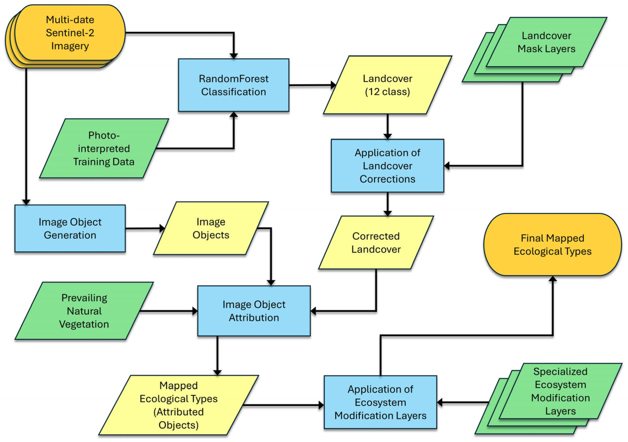
Figure 2.
Prevailing ecological system (potential natural vegetation) for the study area, the state of Arkansas, United States.
Figure 2.
Prevailing ecological system (potential natural vegetation) for the study area, the state of Arkansas, United States.
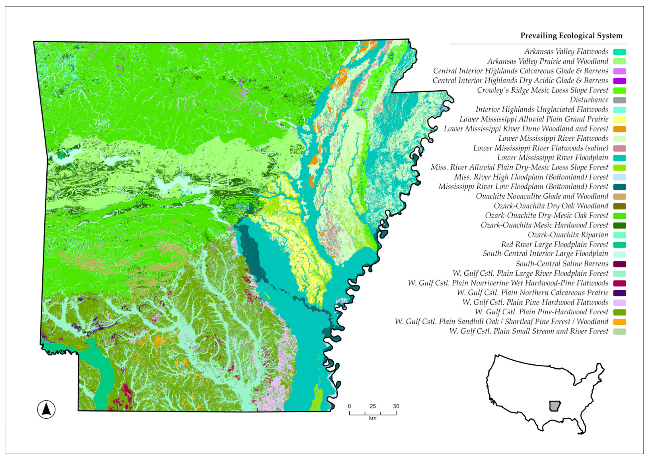
Figure 3.
Mapping zones and corresponding Sentinel-2 satellite orbits used for this study. Classifications were based on 2500 —3000 training data samples per zone.
Figure 3.
Mapping zones and corresponding Sentinel-2 satellite orbits used for this study. Classifications were based on 2500 —3000 training data samples per zone.
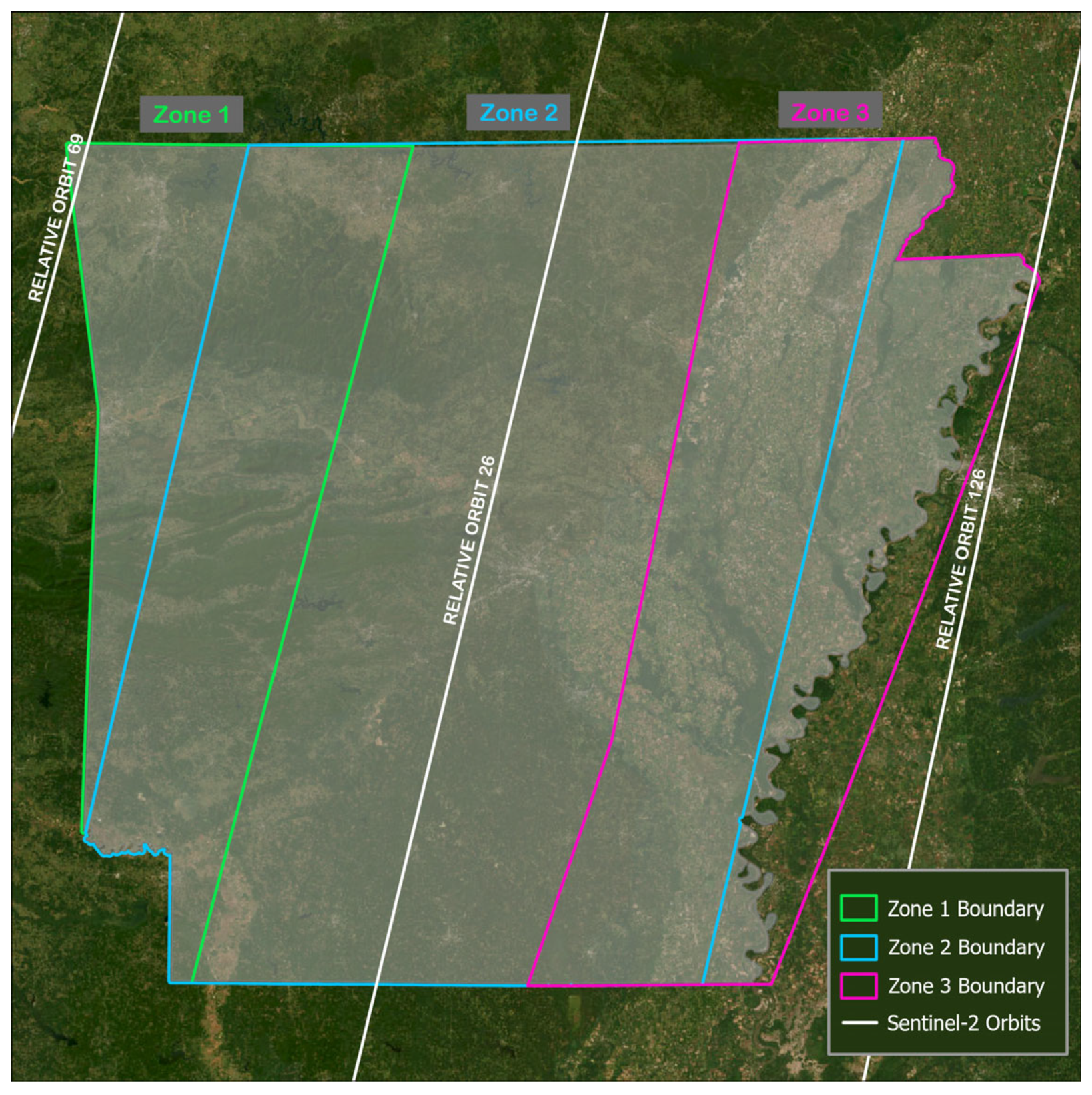
Figure 4.
Final map of statewide ecological system types for Arkansas at 10-meter spatial resolution. The complete list of 123 types is found in Appendix A.
Figure 4.
Final map of statewide ecological system types for Arkansas at 10-meter spatial resolution. The complete list of 123 types is found in Appendix A.
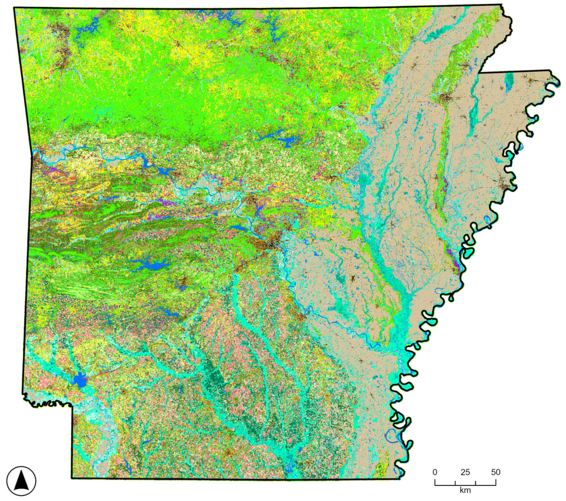

Table 1.
Class targets used for the initial land cover classification.
| Water |
| Developed Impervious |
| Developed Mixed Intensity |
| Barren |
| Row Crops |
| Deciduous Woodland & Forest |
| Deciduous Shrubland & Young Woodland |
| Evergreen Woodland & Forest |
| Evergreen Shrubland & Young Woodland |
| Herbaceous |
| Wet Herbaceous |
| Wooded Wetland & Swamp |
Table 2.
Ecological types accounting for > 1% of statewide cover in the state of Arkansas.
| Ecological Type | Area (ha) | Percent | Description |
|---|---|---|---|
| Ozark-Ouachita Dry-Mesic Oak Forest | 2448995 | 17.52% | This type is mapped over typic soils throughout the Ozark and Ouachita mountain regions. Many areas are closed-canopy forests or nearly so in the modern landscape. Important species include white oak (Quercus alba), hickory species (Carya tomentosa, C. texana), black oak (Q. velutina), post oak (Q. stellata) and chinkapin oak (Q. muehlenbergii, higher pH soils) are characteristic of this type. The most mesic areas may contain sugar maple (Acer saccharum) and northern red oak (Q. rubra) as an important components. Flowering dogwood (Cornus florida), eastern redbud (Cercis canadensis), hophornbeam (Ostrya virginiana), winged elm (Ulmus alata), and sassafras (Sassafras albidum) are common woody understory species. Shortleaf pine (Pinus echinata) may be a component. |
| Row Crops | 2399376 | 17.16% | This type includes all cropland where fields are fallow for some portion of the year in 2021. Some fields may rotate into and out of cultivation frequently, sometimes depending on flooding duration during any given year. |
| Ozark-Ouachita Disturbance Grassland | 931965 | 6.67% | This type circumscribes broad variation, but in the modern landscape most representatives are grazed pastures. Common species are non-native and grazing tolerant grasses and forbs such as Bermudagrass (Cynodon dactylon), tall fescue (Schedonorus arundinaceus), annual ragweed (Ambrosia psylostachya), hogword (Croton capitatus), bromes (Bromus spp.), perennial ryegrass (Lolium perenne), and a variety of grazing tolerate and early successional herbaceous species. Less heavily grazed areas may support grasslands with species such as little bluestem (Schizachyrium scoparium), big bluestem (Andropogon gerardii), and yellow Indiangrass (Sorghastrum nutans). |
| Ozark-Ouachita Pine Woodland and Forest | 534073 | 3.82% | This type is mapped on all soil types where shortleaf pine (Pinus echinata) is dominant in stands that have not been harvested since 1985. White oak (Quercus alba), post oak (Q. stellata), and mockernut hickory (Carya tomentosa) are common components. |
| Mississippi Alluvial Valley and West Gulf Coastal Plain Typic Mature Pine Plantation | 499423 | 3.57% | This type is mapped where mature pines occur in areas that have not been harvested since 1985. These stands include older managed pines, predominantly loblolly pine (Pinus taeda). |
| West Gulf Coastal Plain Large River Floodplain Deciduous Forest | 481492 | 3.44% | This type is mapped on floodplains that have a wide range of hydrologic regimes. Common canopy species include sweetgum (Liquidambar styraciflua), water oak (Quercus nigra), willow oak (Q. phellos), green ash (Fraxinus pennsylvanica), and American elm (Ulmus americana) although numerous other species may be important to dominant components. |
| Floodplain Pine Plantation and Forest | 367744 | 2.63% | This type is mapped on floodplain soils where pines (predominantly loblolly pine, Pinus taeda) are dominant. |
| Open Water | 337799 | 2.42% | This type was open water during all seasons at the time of data acquisition for the current classification (circa 2021) |
| Mississippi River High Floodplain Deciduous Forest | 336139 | 2.40% | This is type is mapped on floodplain soils that were flooded for roughly less than 20% of years since 1983. Common species include willow oak (Quercus phellos), water oak (Quercus nigra), sweetgum (Liquidambar syraciflua), sugarberry (Celtis laevigata), green ash (Fraxinus pennsylvanica), American elm (Ulmus americana), boxelder (Acer negundo), and pin oak (Q. palustris). River front areas may include sycamore (Platanus occidentalis), eastern cottonwood (Populus deltoides), and black willow (Salix nigra) as important species. |
| Pine Plantation (barren, herbaceous, and deciduous shrub cover) | 335052 | 2.40% | This type consists of young pine plantations were harvested between 2011 and 2021, and remain barren or dominated by herbaceous or deciduous shrub cover. In addition to young planted pines, typically loblolly pine (Pinus taeda), species such as sweetgum (Liquidambar styraciflua, central and south), winged elm (Ulmus alata), American beautyberry (Callicarpa americana) sweetgum (Liquidambar styraciflua), red maple (Acer rubra), Rubus spp., Smilax spp., broomsedge bluestem (Andropogon virginicus), and woodoats (Chasmanthium sessiliflorum) are common components. |
| West Gulf Coastal Plain Upland Deciduous Forest | 329597 | 2.36% | This type is mapped on typic upland soils. Common overstory species include post oak (Q. stellata), southern red oak (Q. falcata), black oak (Q. velutina), water oak (Q. nigra), white oak (Q. alba), and mockernut hickory (Carya tomentosa). Common shrubs include hawthorns (Crataegus spp.), American beauty berry (Callicarpa americana), Vaccinium spp., Viburnum spp., and Rubus spp. |
| Ozark-Ouachita Mature Pine Plantation | 327478 | 2.34% | This type consists mainly of mature pine plantations (Pinus echinacea or P. taeda) or dense pine stands that were harvested between 1985 and 2011. |
| Mississippi Alluvial Valley and West Gulf Coastal Plain Typic Young Pine Plantation | 318116 | 2.28% | The type is mapped mainly in the Crowley's Ridge and Grande Prairie ecoregions, in areas that are higher in elevation than the Mississippi Alluvial Valley plain surface. Common trees include white oak (Quercus alba), mockernut hickory (Carya tomentosa), Texas hickory (Carya texana), northern red oak (Quercus rubra, Crowley's Ridge), southern red oak (Quercus falcata), cherrybark oak (Quercus pagoda), post oak (Quercus stellata), Shumard oak (Quercus shumardii), and black oak (Quercus velutina). Winged elm (Ulmus alata) and hophornbeam (Ostrya virginiana) are common in the understory. |
| South-Central Interior Large Floodplain Deciduous Forest | 203247 | 1.45% | This type is mapped on bottomland soils across a variety of hydrologic regimes and various stages of disturbance. Common canopy dominants may include ash species (Fraxinus americana, F. pennsylvanica), elm species (Ulmus americana, U. rubra), sweetgum (Liquidambar styraciflua), sycamore (Platanus occidentalis), sugarberry species (Celtis laevigata), black willow (Salix nigra), boxelder (Acer negundo), Shumard oak (Quercus shumardii), and bur oak (Quercus macrocarpa). Vines such as eastern poison ivy (Toxicodendron radicans), grape species (Vitis spp.), Virginia creeper (Parthenocissus quinquefolia), and greenbriar (Smilax spp.) species may be conspicuous components. |
| Mississippi Alluvial Valley and West Gulf Coastal Plain Typic Pine Woodland and Forest | 196193 | 1.40% | This type consists of pine plantations that were harvested within the 11 years prior to 2021, replanted, and are now dominated by young pine. Loblolly pine (Pinus taeda) is the most common species. |
| West Gulf Coastal Plain Upland Disturbance Grassland | 191177 | 1.37% | This type is mapped on typic upland soils. In the modern landscape, these areas often represent grazed pastures or hay fields. Bermudagrass (Cynodon dactylon) is commonly encountered. |
| Mississippi River Low Floodplain Deciduous Forest | 161834 | 1.16% | This type is mapped on floodplain soils that were flooded in roughly more than 20% of years since 1983. Common species include willow oak (Quercus phellos), sweetgum (Liquidambar syraciflua), overcup oak (Q. lyrata), water hickory (Carya aquatica), green ash (Fraxinus pennsylvanica), sugarberry (Celtis laevigata), American elm (Ulmus americana), slippery elm (Ulmus rubra), and pin oak (Q. palustris). |
| Ozark-Ouachita Dry-Mesic Deciduous Shrubland and Young Woodland | 154289 | 1.10% | This type represents a variety of young, sparse woodlands, woodland edges, and shrublands. Common woody species are young trees from the Ozark-Ouachita Dry Woodland. Other species may include winged elm (Ulmus alata), sugarberry (Celtis laevigata), sassafras (Sassafras albidum), redbud (Cercis canadensis), red maple (Acer rubrum), hophornbeam (Ostrya virginiana), and Prunus spp. Vines such as poison ivy (Toxicodendron radicans), Virginia creeper (Parthenocissus quinquefolia), greenbrier species (Smilax spp.) and blackberry species (Rubus spp.) are common. |
| Mississippi Alluvial Valley Dry-Mesic Loess Deciduous Forest | 151914 | 1.09% | This type is mapped in the same area as the Mississippi Alluvial Valley Dry-Mesic Loess Deciduous Forest and may consist of young or sparse woodlands, often with successional trees and shrubs. Common woody species may include post oak (Quercus stellata), black oak (Q. velutina), white oak (Q. alba), hickory species (Carya spp.), winged elm (Ulmus alata), sugarberry (Celtis laevigata), common persimmon (Diospyros virginiana), sassafras (Sassafras albidum), black cherry (Prunus serotina), redbud (Cercis canadensis), and Prunus spp. Vines such as poison ivy (Toxicodendron radicans), Virginia creeper (Parthenocissus quinquefolia), greenbrier species (Smilax spp.) species, and blackberry species (Rubus spp.) are common. |
| Ozark-Ouachita Young Pine Plantation | 148380 | 1.06% | This type consists of areas dominated by young pines in stands that are fewer than 11 years old as of 2021. |
Disclaimer/Publisher’s Note: The statements, opinions and data contained in all publications are solely those of the individual author(s) and contributor(s) and not of MDPI and/or the editor(s). MDPI and/or the editor(s) disclaim responsibility for any injury to people or property resulting from any ideas, methods, instructions or products referred to in the content. |
© 2024 by the authors. Licensee MDPI, Basel, Switzerland. This article is an open access article distributed under the terms and conditions of the Creative Commons Attribution (CC BY) license (http://creativecommons.org/licenses/by/4.0/).
Copyright: This open access article is published under a Creative Commons CC BY 4.0 license, which permit the free download, distribution, and reuse, provided that the author and preprint are cited in any reuse.


