
Submitted:
02 October 2024
Posted:
07 October 2024
You are already at the latest version
Abstract
The reliable operation of power systems depends on rapid fault detection to trigger protection mechanisms and prevent further damage. Machine Learning-based fault detection systems have gained prominence for their superior performance. These automated systems can assist operators by highlighting anomalies and faults, providing a robust framework for improving Situation Awareness. However, existing approaches predominantly rely on monolithic models, which struggle with adapting to changing data, handling imbalanced datasets, and capturing patterns in noisy environments. To overcome these challenges, this study explores the potential of Multiple Classifier System (MCS) approaches. The results demonstrate that ensemble methods generally outperform single models, with dynamic approaches like META-DES showing remarkable resilience to noise. These findings highlight the importance of model diversity and ensemble strategies in improving fault classification accuracy under real-world, noisy conditions. This research emphasizes the potential of MCS techniques as a robust solution for enhancing the reliability of fault detection systems.
Keywords:
electrical transmission systems
; situation awareness
; fault detection
; multiple classifier systems
; ensemble
; dynamic classifier selection
1. Introduction
Electrical power systems are vital to the functioning and advancement of modern societies, providing energy to critical infrastructure and services, including telecommunications, transportation, water supply, and emergency response systems [1,2,3]. Modern power systems consist of various electrical components [4], which are dynamic and susceptible to disturbances or failures. These failures may result from internal network issues, such as short circuits, or external factors, such as environmental conditions [5]. Large power generation plants must operate in synchronization with electrical grids, making it essential that the entire energy system functions safely and efficiently. In this context, fault detection is crucial, as it enables the prompt activation of protective measures, protecting equipment and preventing further damage to the network [6,7].
Fault detection is crucial in improving Situation Awareness (SA) in energy systems. In this context, SA involves perceiving, understanding, and predicting changes within power systems [8,9]. SA supports operators and automated systems in understanding the system’s current state, detecting potential issues, and predicting future states. According to [10], the first level of SA is the perception of critical elements in the environment. In energy systems, this involves monitoring sensors, performance data, and operational parameters to detect when something is wrong—such as abnormal voltage, temperature spikes, or power outages [11]. Automated fault detection algorithms assist operators by highlighting anomalies that may indicate a fault. In this sense, energy operators can better manage system reliability and prevent cascading failures by integrating advanced fault detection systems (such as Machine Learning (ML) models and real-time monitoring) with a robust framework for SA. Enhanced SA improves the speed and accuracy of response to faults, reducing downtime and improving overall system resilience.
Numerous studies in the literature have applied a range of Machine Learning (ML) models for fault classification in transmission lines, including Decision Trees [12], Random Forests [13], XGBoost [14], CatBoost [15], LightGBM [16], and K-Nearest Neighbors (KNN) [17]. These models have been successfully applied to classify faults based on voltage and current signals. However, the performance of these ML models often considerably deteriorates when exposed to noisy data or signal distortions [18] due to issues related to overfitting, underfitting, and model selection. In this context, Multiple Classifier Systems (MCS) are a promising alternative to address the limitations of single (or monolithic) approaches, improving the robustness and accuracy of fault classification models. MCS consists of a set of models, each specialized in recognizing different patterns, which are selected and combined to achieve a final classification. The motivation behind this approach is that no single model performs optimally across all possible scenarios [19].
Few studies have applied MCS, also known as ensemble approaches, to fault classification in electrical transmission systems [18,20,21,22,23]; most have focused on traditional approaches such as Bagging or Boosting [18,23]. These approaches combine the output of multiple models to improve overall accuracy but consider each classifier equally across the dataset. Conversely, relevant results in classification tasks [24] have been obtained by selecting specific classifiers for each test pattern, a technique known as dynamic classifier selection, as well as by combining models through stacking, which generates a meta-model that learns to combine the models in an ensemble, resulting in more accurate classifications [25]. This gap highlights the need to investigate whether MCS approaches, such as stacked learning and dynamic classifier selection, can significantly improve the performance of fault classification in electrical transmission systems, particularly in noisy data.
This work investigates the effectiveness of ensemble learning approaches, specifically stacking models and dynamic classifier selection. To achieve this, MCSs were developed, each employing a different approach to perform the final classification. These methods are compared against traditional single models, such as Decision Tree, KNN, and XGBoost, to determine whether ensembles can offer superior performance under different noisy data conditions. Different levels of noise were introduced into the datasets to assess the robustness of the approaches.
The contributions of this work include:
- Evaluation of well-established MCS approaches from the literature in the fault classification in electrical transmission systems task;
- Assessment of the impact on the performance of static ensemble and dynamic selection approaches when different levels of noise are introduced;
- Comparison of the MCS with various single models from the literature across 14 different scenarios in total;
- The superior performance of dynamic selection approaches to deal noise and enhancing classification accuracy regarding single models.
2. Multiple Classifier Systems
Multiple Classifier System (MCS), or Ensemble Learning, is an area of ML highlighted due to remarkable theoretical and practical results [26]. Ensemble-based approaches aim to reduce the overall susceptibility of the single ML models to bias and variance by combining multiple models, making them more robust. Therefore, these approaches must consider how they group models, combining them to minimize their drawbacks in the final ensemble. The superiority of the ensembles against single approaches has been demonstrated across several real-world problems, such as credit scoring [27], heart disease classification [28], correlative microscopy [29], fault classification [30], fingerprint analysis [31] and others applications [32]. The main motivation for using MCS is based on the No Free Lunch theorem, which states that no single model is the best for all classes of real-world problems [19].
An MCS comprises three phases: generation, selection, and integration. In the generation phase, a pool of classifiers is created. The generated pool must be accurate and diverse [33]. The diversity occurs when the pool models provide different performances for the same patterns. Several strategies can be employed to introduce diversity into the model pool, such as using different training samples, varying classifier types, selecting different features, or tuning distinct parameters for each classifier [33].
In the selection phase, one or more models are chosen based on a predefined criterion. This choice can be performed in two ways: Static Selection (SS) (Figure 1), or Dynamic Selection (DS) (Figure 2). In the first, the same set of models is used to classify all new instances in the test set. In the second, one specific model or set of models is chosen for each new instance.
When more than one classifier is selected, the outputs must be combined, making the integration phase necessary. In this phase, an aggregation strategy is applied to combine all outputs to generate the final classification for a given new pattern. For this phase, we evaluate two widely used approaches in the literature: majority voting [34] and stacked generalization [35].
In this work, we evaluate unprecedent way different MCS approaches for electrical fault detection task. Figure 1 and Figure 2 show the MCS frameworks evaluated in static and dynamic ensemble, respectively.
2.1. Static Ensemble
In the static ensemble (Figure 1), the entire set of classifiers in the pool is considered for the final classification. The MCS developed in this work consists of two phases: (a) training and (b) testing. In the training phase, a set of classifiers , where n is the size of the pool, is trained using the training dataset, resulting in a pool . In the case of a stacked model, the outputs of the pool for the training dataset are sent as input to train an aggregation model A, which learns to combine the classifications from the pool. The output of this phase is the pool containing the base classifiers and the aggregation function that will be applied during the combination step.
In the testing phase, each new instance is passed to the pool, which returns , a set of n classifications, one from each model. The aggregation function is then applied to combine these classifications and produce the final classification.
As Aggregation Functions, we evaluated two approaches that are widely used in static ensemble methods: majority vote and stacked generalization. Majority vote method, introduced by Breiman (1996) [36], consists of each base classifier predicting a class for a new data instance, with the final prediction determined by the class that receives the highest number of votes. This method enhances overall predictive performance, making it particularly effective for unstable models where small changes in the training data can lead to significant variations in predictions [37].
Stacked generalization, introduced by Wolpert (1992) [38], involves training a meta-classifier to combine the predictions from base classifiers. This meta-classifier is trained using the outputs of the base models on the training sample. During inference, for a new pattern, the predictions of the base models are used as inputs to the meta-classifier, which then combines them to return the final prediction. This method enables the meta-classifier to effectively leverage the strengths of diverse base models, leading to improved predictive performance and robustness when these models exhibit high variability [25]. In this work, we evaluate two algorithms as meta-classifiers: Decision Tree and Logistic Regression, both of which are used in stacked generalization [25,39].
2.2. Dynamic Ensemble
In the dynamic ensemble (Figure 2), a subset of classifiers from the pool is selected for each new test instance. This subset can be composed of one to n classifiers, where n is the size of the pool. The MCS developed in this work consists of two phases: (a) training and (b) testing. The training phase is composed of two steps: Classifier Generation and Meta-Classifier Generation. In the Classifier Generation step, similar to the static ensemble, a pool of n classifiers is generated. The Meta-Classifier Generation step is executed only when the dynamic selection approach requires a meta-classifier to select the best model. In this step, the training samples are used to extract meta-features, and the algorithm M is applied to generate the Meta-Classifier.
The testing phase consists of three steps, and the path to the final classification depends on the chosen dynamic selection approach. The first step is the RoC (Region of Competence) creation, which is executed by dynamic approaches that require a Region of Competence. The RoC is created using the validation instances most similar to the new test instance, to select the set of models with the best performance for classifying instances within this RoC. The second step is "Classifiers Evaluation," which involves selecting the set of models based on specific criteria. Most approaches select classifiers based on their performance within the Region of Competence. However, we also evaluate the use of a Meta-Classifier, which extracts meta-features from the new instance and selects the set of models best suited to classify it. The output of this step is a set S of selected models, which can range from 1 to N models. Finally, in the classification step, the output of each model in the selected set is obtained. If only one classifier is selected, its classification is returned as the final classification (). However, if more than one model is selected, the is achieved through majority voting in the final step.
In this work, we evaluate six state-of-the-art dynamic selection algorithms: OLA, DESP, KNORA-E, KNORA-U, MCB, and M-DES.
2.2.1. DCS-LA
Dynamic Classifier Selection by Local Accuracy (DCS-LA), also known as Overall Local Accuracy (OLA), introduced by Woods et al. (1997) [40], is a method for selecting the most competent classifier for each test sample based on local accuracy estimates within a Region of Competence (RoC). For each test instance, the RoC, composed of the k-nearest neighbors from the training set that are most similar to the new instance, is created. Then, the classifier with the highest accuracy within the RoC is selected to return the final classification.
2.2.2. DESP
Dynamic Ensemble Selection Performance (DESP) method, introduced by Woloszynski et al. (2012) [41], consists of selecting the classifiers that achieve a classification performance in the RoC, superior to a Random Classifier (RC). The performance of the RC is defined as , where L is the number of classes in the problem. If no base classifiers achieve this criterion, then the full pool is utilized for classification, and the final classification is achieved through the majority voting method.
2.2.3. KNORA-E
K-Nearest Oracles Eliminate (KNORA-E) method, introduced by Ko et al. (2008) [42], consists of selecting classifiers that correctly classify all instances within the RoC. If no classifier correctly classifies all the samples in this region, then the size of the region is reduced until at least one classifier meets the criterion. If still no classifiers meet the criterion, the full pool is utilized. The final decision is made using the majority voting method.
2.2.4. KNORA-U
K-Nearest Oracles Union (KNORA-U) method, as introduced by Ko et al. (2008) [42], involves selecting classifiers that correctly classify at least one instance within the Region of Competence (RoC). Each selected classifier is assigned a weighted vote based on the number of instances it correctly classifies within the RoC. The final decision is made by the class that accumulates the most votes from the selected classifiers.
2.2.5. MCB
Multiple Classifier Behavior (MCB) method, introduced by Giacinto and Roli (2001) [43], consists of dynamically selecting classifiers based on their local accuracy within a RoC, which is determined using similarity metrics and the concept of Behavioral Knowledge Space (BKS). The behavior of classifiers is represented by an MCB vector, which includes the class predictions made by each classifier for the test instance. The similarity between the MCB vector of the test instance and those of its neighbors is then computed. Neighbors with a similarity above a certain threshold are used to refine the RoC. Finally, the classifier with the highest accuracy within this refined RoC is chosen to make the final classification.
2.2.6. META-DES
META-DES method, introduced by Cruz et al. (2014) [44], consists of dynamically selecting classifiers based on multiple criteria that assess the competence of each classifier.
In the training phase, a meta-classifier is generated through a meta-feature extraction process. This process involves generating multiple sets of meta-features, each representing a different criterion related to the performance of the base classifiers, such as their local accuracy, consensus in predictions, and confidence level for the input sample. These meta-features are then used to train the meta-classifier, which learns to predict whether a base classifier is competent enough to correctly classify new test instances.
In the testing phase, for each instance, the meta-classifier predicts whether a base model is competent to classify it; if more than one classifier is selected, the final classification is achieved through the majority voting method.
3. Experimental Protocol
This section is organized into two subsections: Dataset Description (Section 3.1) and Experimental Setup (Section 3.2). Section 3.1 provides detailed information about the two datasets used in the experiments, while Section 3.2 outlines the protocol followed to evaluate the single and ensemble approaches in this study.
3.1. Dataset Description
Two separate datasets were used to evaluate the single and ensemble approaches discussed in this paper. The first dataset, referred to here as Dataset 1, was generated using ATPDraw software1. This dataset simulates the 138 kV section of a substation, including two transmission lines connected to the substation bus. Each line was considered as a load of 36 MW and 18 Mvar. Various types of faults were simulated between circuit breakers and line outputs, covering phase-to-ground, phase-to-phase, phase-to-phase-to-ground, and three-phase faults. Current measurements were taken at the transformer connection breaker on the main bus and at the line connection breakers sharing the same bus. Additionally, the voltage at the line outputs was measured. The simulation lasted 200 seconds, with data collected at 0.01-second intervals, resulting in a database of 20,000 samples. This database is structured as follows: the features columns represent voltage measurements at the outputs of the two lines for phases A, B, and C. Following these columns are current measurements in the circuit above the circuit breakers. The classes are categorized as follows:
- Class 0: No faults
- Class 1: Phase-to-ground faults
- Class 2: Phase-to-phase faults
- Class 3: Phase-to-phase-to-ground faults
- Class 4: Three-phase faults
The second dataset (referred to as Dataset 2), derived from [45], was adapted to include only the energy variables of current and voltage signals, along with their Root Mean Square (RMS) values. As the system is three-phase, the final database contains twelve attributes and two variables that can be used as targets: fault location and fault type. The first is used to locate where the fault occurred and has discrete values between 4.14 and 414, each representing a distance in kilometers. The second variable has categorical values indicating the phases in which the fault occurred, such as AB, BC, and BG. In the present work, fault type was used as the target. The classes are categorized as follows:
- Class 0: Fault AB
- Class 1: Fault ABC
- Class 2: Fault ABG
- Class 3: Fault AC
- Class 4: Fault ACG
Gaussian noise was introduced during preprocessing to better approximate real-world conditions and evaluate the robustness of the models. For the first dataset, noise values ranged from 10,000 to 60,000. In the second dataset, due to the extremely high original values (in the megawatt range), we normalized the data by dividing by 100,000, resulting in Gaussian noise values between 0.1 and 1.5.
Each dataset was divided into two distinct samples: 80% for training and 20% for testing. This split ensures that the models have sufficient data to learn from while preserving a portion for evaluating the generalization power of approaches on unseen data.
3.2. Experimental Setup
The static ensemble and dynamic selection approaches were evaluated using the two datasets previously described. All selected approaches are well-established in the ensemble learning literature and have achieved notable results in various application domains [33,46,47,48]. This study assessed the following static ensemble methods: Majority Vote, Stacked Decision Trees (DT), and Stacked Logistic Regression (LR). For dynamic selection, we evaluated the following approaches: DESP, KNORA-E, KNORA-U, MCB, M-DES, and OLA. Table 1 and Table 2 show the hyperparameters used for static ensembles and dynamic selection approaches, respectively. The hyperparameters employed are the default values of the Python language’s DESlib package 2.
The static and dynamic ensemble approaches are compared against six individual classification models. To ensure a fair comparison, these classification models are also included in the pool of classifiers used in the evaluated ensembles. The individual models are described in detail below.
A Decision Tree (DT) is a supervised learning model that uses a rule-based approach to build a binary tree structure for decision-making. A DT maps a data domain to a response set by recursively dividing the domain into subdomains, ensuring that each division gains more significant information than the original node [49]. The final structure of a DT consists of decision nodes and leaf nodes. The DT is a white-box model for classification, offering the advantage of transparency in its decision-making process. This transparency is achieved by interpreting the tree’s rules, which reveal the logical path behind each prediction [50,51].
Random Forest (RF) is an ensemble learning model composed of multiple decision trees. During training, each tree is built on a different subset of the training data, selected using the bagging technique (random sampling with replacement). This process introduces diversity among the trees, producing independent and uncorrelated models, which helps reduce overfitting and improves generalization [52]. In the testing phase, the final classification is determined by a majority vote from all the trees, with the class receiving the most votes selected as the final prediction [13].
Gradient Boosting (GB) based models create an ensemble using the boosting technique, where new classifiers are trained based on the residuals of the current model. These models employ gradient descent to minimize the loss function by iteratively adding models that correct the residuals of the combined ensemble. The main algorithms in this category are Extreme Gradient Boosting (XGBoost) [14], Light Gradient Boosting Machine (LightGBM) [16], and CatBoost [15]. XGBoost is designed to optimize both computational speed and model performance. This model adds regularization terms to control the complexity of the model, which is helpful to prevent over-fitting and improve the generalization of the model. LightGBM is similar to XGBoost but employs a distinct leaf-wise tree growth strategy. This method enables LightGBM to grow trees in a manner that more effectively reduces loss, often resulting in faster training times and improved accuracy. CatBoost is a classifier that simplifies data preparation by effectively handling missing values for numerical variables and non-encoded categorical variables, reducing the need for extensive preprocessing. Unlike XGBoost and LightGBM, which require manual encoding of categorical features, CatBoost processes these features natively, leading to potentially better performance and more straightforward implementation.
K-Nearest Neighbors (KNN) is a lazy learning model with no training process. KNN works by locating the K data points in the training sample most similar to a new data point, forming a “nearest neighbors region”, and making a prediction based on this region. In the case of a classification task, for each new data point, KNN assigns a class by determining the majority class among the nearest neighbors [17,53].
Table 3 shows the hyperparameter values for each model evaluated. These values were selected based on previous works that addressed electrical fault detection tasks using ML models [12,13,14,15,16,17]. The hyperparameters for each model were selected through grid search cross-validation with five folds. This technique helps mitigate overfitting by ensuring the models are evaluated on multiple subsets of the data. For each set of values from the grid search, the training data is split into five equal parts. During each iteration, four parts are used for training while the remaining part is used for validation. The combination of hyperparameter values with the highest mean accuracy is selected.
The evaluation of the models was conducted using three well-known metrics: Accuracy, Precision, and Recall. Accuracy measures the overall correctness of the model, providing a general measure of how well the model performs across all classes. Precision and Recall, on the other hand, offer insights into the model’s performance specifically on the positive class. Precision focuses on the correctness of positive predictions, indicating the proportion of true positive results among all positive predictions. Recall assesses the completeness of positive predictions, representing the proportion of true positive results out of the actual positive cases. Table 4 presents the equations, ranges, and acronyms for each metric. True Positive (TP) refers to instances where the model correctly predicts the positive class. True Negative (TN) refers to instances where the model correctly predicts the negative class. False Positive (FP) occurs when the model incorrectly predicts the positive class for a negative instance. False Negative (FN) occurs when the model incorrectly predicts the negative class for a positive instance.
4. Results
The following sections (Section 4.1 and Section 4.2) analyze the experimental results of the evaluated approaches, encompassing single, static ensemble, and dynamic selection models for the two used datasets. The approaches are evaluated using the metrics of Accuracy (A), Precision (P), and Recall (R) in seven and eight scenarios for Datasets 1 and 2, respectively.
4.1. Dataset 1
Table 5 shows the metrics (A, P, and R) used to analyze the performance of the single models. In general, the values of metrics A, P, and R decreased as the noise level increased. RF and KNN achieved the highest A, P, and R values in the noise-free scenario, while DT recorded the lowest values. Nevertheless, KNN was the model that was more affected by the increase in the noise level. Indeed, KNN obtained the second worst result from noise level 10,000 to 60,000. This result shows the KNN’s sensibility to noisy data. DT obtained the worst values in all scenarios. This poor result can be caused by overfitting in the training sample or class imbalance.
LightGBM, XGBoost, and CatBoost, ranked first, second, and third respectively, demonstrated more stable performance with the addition of noise. All three models achieved A, P, and R values exceeding 99% across all scenarios. This result shows that these gradient-boosting algorithms are able to handle noisy data by iteratively refining their predictions, which allows them to maintain robustness in the presence of noise.
Figure 3 shows the evolution of accuracy for the different noise levels. It is possible to note the performance degradation of all models, mainly KNN, DT, and RF, respectively.
Table 6 shows the A, P, and R metrics attained by the static ensemble models (Majority Vote, Stacked DT, and Stacked LR). For all models, the metric values tend to decrease with the increase in the noise level. Both Stacked models attained a more stable result, varying around 99% for all metrics. This result shows that the strategy of assigning weights was effective. Indeed, the single models LightGBM, XGBoost, and CatBoost reached the best results and, therefore, received the highest weights in the Stacked ensembles. Conversely, the addition of noise negatively impacted the Majority Vote model, with the A, P, and R metrics dropping from 99.90% across the board to 97.92%, 98.00%, and 97.92%, respectively. This result shows that the DT, KNN, and RF models must have influenced the decision of the Majority Vote. This result shows the importance of the pool’s quality (creating and training) and the combination strategy. Figure 4 shows the evolution of accuracy for the different noise levels. The performance degradation of all models, mainly of the Majority Vote, can be noted.
Table 7 shows the performance of the Dynamic Selection models (DESP, KNORA-E, KNORA-U, MCB, M-DES, and OLA) for Dataset 1. For all models, the metric values tend to decrease with the increase in the noise level. KNORA-E, KNORA-U, and M-DES reached a more stable performance, varying all metrics around 99%. On the other hand, the OLA model suffered from increasing noise since the A, P, and R metrics decreased from 99.90%, 99.90%, and 99.90% to 94.97%, 95.11%, and 94.97%. These results show that methods based on the Region of Competence (RoC), which rely on training instances similar to the test instance, like OLA exhibit higher sensitivity to noise. In contrast, performance-based approaches, such as those employed by KNORA-E and KNORA-U, or the use of meta-features like the M-DES approach, demonstrate greater robustness. Figure 5 shows the evolution of accuracy for the different noise levels. The performance degradation of all models, mainly of the DESP, MCB, and OLA, can be noted.
Figure 6 compares the metric values reached by the best models of the evaluated approaches: Single Models, Static Ensemble, and Dynamic Selection. It shows that models based on ensembles attained the best results in all scenarios. From the Without Noise scenario until 50,000 Amp, Stacked LR attained the best A, P, and R values; meanwhile, for 60,000 Amp, M-DES was superior for all metrics. It is essential to highlight that ensemble approaches attained higher performance values than single models in most scenarios. For instance, Stacked LR and M-DES reached a superior performance of around 48% and 41% in terms of A for DT and KNN, respectively.
In summary, the results for Dataset 1 demonstrate that the MCS approaches consistently outperformed single models in most scenarios, particularly in the presence of noise. Among the single models, gradient-boosting methods such as LightGBM, XGBoost, and CatBoost showed a more stable performance, maintaining high metric values even as the noise level increased, while KNN and DT were the most affected by the noise. Static ensemble models, especially Stacked LR, proved to be effective in maintaining robust performance across noise levels, benefiting from the weighted combination of high-performing models. In the dynamic selection approaches, KNORA-E, KNORA-U, and M-DES demonstrated resilience to noise, maintaining nearly consistent performance. The performance degradation of methods like OLA, MCB, and DESP highlights their sensitivity to noise. Thus, the MCS approaches evaluted, particularly Stacked LR and M-DES, provided the best results, validating the effectiveness of combining and selection models to enhance robustness and accuracy in noisy environments.
4.2. Dataset 2
Table 8 shows the A, P, and R performance metrics reached by the single models for Dataset 2. The A, P, and R metrics values for all evaluated models have a downward trend with the increase in the noise level. XGBoost and LightGBM models reached the best metric values in all scenarios. LightGBM attained the first rank in the two first scenarios, while XGBoost was the best one in the others. Both reached the same performance for a noise level of 0.3 (third scenario). KNN and DT obtained the two worst metric values for all scenarios in this order. However, between them, the KNN performance was more affected by the increase in the noise level. For instance, the A value of the KNN and DT models dropped 11.90% and 16.78%, respectively. This result shows the KNN’s sensibility to noisy data and a probable overfitting of the DT in the training sample. Figure 7 shows the degradation of all single models in terms of the A metric with the increase in the noise level. It is evident that KNN and DT produced the poorest results. However, CatBoost, LightGBM, RF, and XGBoost were the models most affected by the increasing noise levels.
Table 9 shows the A, P, and R metrics attained by the static ensemble models. For all models, the metric values tend to decrease with the increase in the noise level. These results show that the Stacked LR and Majority Vote models demonstrate greater robustness across all noise levels. Initially, Stacked LR outperforms Majority Vote, delivering superior results with 99.80% of A, P, and R in the noise-free scenario, compared to 99.66% obtained by Majority Vote. However, from noise level 0.5, Majority Vote showed competitive performance, with 78.58% of accuracy at noise level 1.5, closely matching Stacked LR, which achieved 78.34% under the same conditions. In contrast, Stacked DT showes to be the most sensitive to noise, starting with a highlighted performance of 99.77% in the noise-free scenario but dropping significantly to 70.55% at noise level 1.5. This behaviour likely occurred due to the nature of DT, which are prone to overfitting, especially when confronted with noisy data. As noise increases, the trees within the ensemble may capture random fluctuations, leading to poorer generalization and significant performance degradation. Figure 8 shows the evolution of accuracy for the different noise level, mainly Stacked DT, can be noted.
Table 10 shows the performance of the Dynamic Selection approaches (DESP, KNORA-E, KNORA-U, MCB, M-DES, and OLA) for Dataset 2. KNORA-E, KNORA-U, and M-DES exhibited more stable performance, starting with accuracy around 99% in the noise-free scenario, but decreasing to approximately 77% at a noise level of 1.5. The DESP model showed competitive performance starting from noise level 0.5, achieving a recall of 84.77, compared to 84.19 for KNORA-U and 83.99 for M-DES. In contrast, OLA and MCB were more sensitive to noise, with OLA showing the most significant performance drop due to its reliance on local training instances, which become less reliable as noise increases.
Figure 9 shows the evolution of accuracy for the different noise levels. The performance degradation of all models, mainly of the MCB and OLA, can be noted.
Figure 10 compares the metric values achieved by the best models from the evaluated approaches: Single Models, Static Ensemble, and Dynamic Selection for the Dataset 2. The figure shows that, initially, with no noise (), all models performed similarly, with metrics above 95%. As noise levels increase, Stacked LR exhibits a sharper decline compared to XGBoost and META-DES, which maintain better resilience. From onwards, the degradation becomes more pronounced for all models, with META-DES and XGBoost consistently outperforming Stacked LR, particularly in terms of precision and recall, demonstrating greater robustness to noise.
In summary, the results for DataSet 2 indicate that the ensemble and dynamic selection approaches consistently outperformed single models as noise levels increased. Among the single models, XGBoost and LightGBM demonstrated greater resilience, maintaining strong performance across various noise levels, while KNN and DT were the most affected by the noise, with KNN showing higher sensitivity. Static ensemble models, particularly Stacked LR and Majority Vote, exhibited robust performance, with Stacked LR excelling in noise-free conditions and Majority Vote showing competitive performance as noise increased. In the dynamic selection approaches, KNORA-E, KNORA-U, and M-DES demonstrated stability and resilience, while OLA and MCB experienced significant performance degradation under noisy conditions. Overall, M-DES and XGBoost were the most robust models, consistently providing superior results, validating the effectiveness of ensemble and dynamic selection methods in enhancing model performance and robustness in the presence of noise.
5. Conclusions
This work explored the application of Multiple Classifier Systems for fault classification in electrical transmission systems. Ensemble approaches, particularly Stacked and M-DES, consistently outperformed traditional single models, such as Decision Tree and K-Nearest Neighbors, demonstrating remarkable resilience in noisy environments. The robustness of gradient boosting models, such as LightGBM, XGBoost, and CatBoost, was evident, maintaining high accuracy levels even with the introduction of significant noise. Additionally, dynamic selection approaches, especially KNORA-E, KNORA-U, and M-DES, proved more effective at handling noise than static approaches. These findings highlight the potential of ensemble approaches in improving fault detection accuracy in challenging conditions, as well as the importance of model diversity and combination strategies in enhancing classification performance when dealing with noisy data. Besides, ensemble-based systems employed for fault detection can be a helpful tool in increasing Situational Awareness in electrical power systems.
For future works, dynamic classifier selection and combination approaches could be proposed to handle even higher levels of noise or to apply these techniques to different types of faults and other components of electrical power systems.
Author Contributions
Conceptualization, J.W., D.P., E.S. and P.N.; methodology,J.W., D.P., E.S. and P.N.; experimental process, J.W., D.P., D.C., J. M., E.S. and P.N.; Formal Analysis J.W., D.P., E.S. and P.N.; writing—original draft preparation, J.W. and D.P.; writing—review and editing, E.S. and P.N.; supervision, P.N; funding acquisition, P.N. All authors have read and agreed to the published version of the manuscript.
Funding
“The research was funded by the the Programa de Pesquisa Desenvolvimento e Inovação da Agência Nacional de Energia Elétrica (PD&I ANEEL) and the EVOLTZ company.”
Data Availability Statement
The original contributions presented in the study are included in the article and further inquiries can be directed to the corresponding author.
Acknowledgments
This study was funded by the Research and Development and Innovation (R&D&I) Program regulated by the National Electric Energy Agency (ANEEL-PD-06908-0002/2021) as well as the company EVOLTZ, under the project "Improvement of Operator Situational Awareness using Data Mining and Artificial Intelligence Techniques." This work also received support from the National Council for Scientific and Technological Development (CNPq) and the Coordination for the Improvement of Higher Education Personnel (CAPES). The authors would like to thank the Federal University of Pernambuco (UFPE) and the Advanced Institute of Technology and Innovation (IATI), Brazil.
Conflicts of Interest
The authors declare no conflicts of interest.
References
- O’Rourke, T.D. Critical infrastructure, interdependencies, and resilience. BRIDGE-Washington-National Academy of Engineering- 2007, 37, 22.
- Dobson, I.; Carreras, B.A.; Lynch, V.E.; Newman, D.E. Complex systems analysis of series of blackouts: Cascading failure, critical points, and self-organization. Chaos: An Interdisciplinary Journal of Nonlinear Science 2007, 17. [CrossRef]
- Yagan, O.; Qian, D.; Zhang, J.; Cochran, D. Optimal allocation of interconnecting links in cyber-physical systems: Interdependence, cascading failures, and robustness. IEEE Transactions on Parallel and Distributed Systems 2012, 23, 1708–1720. [CrossRef]
- Goni, M.F.; Nahiduzzaman, M.; Anower, M.; Rahman, M.; Islam, M.; Ahsan, M.; Haider, J.; Shahjalal, M. Fast and Accurate Fault Detection and Classification in Transmission Lines using Extreme Learning Machine. e-Prime - Advances in Electrical Engineering, Electronics and Energy 2023, 3, 100107. [CrossRef]
- Janarthanam, K.; Kamalesh, P.; Basil, T.V.; Kovilpillai, A.K.J. Electrical Faults-Detection and Classification using Machine Learning. 2022 International Conference on Electronics and Renewable Systems (ICEARS), 2022, pp. 1289–1295.
- Jamil, M.; Sharma, S.K.; Singh, R. Fault detection and classification in electrical power transmission system using artificial neural network. SpringerPlus 2015, 4, 1–13. [CrossRef]
- Lusková, M.; Leitner, B. Societal vulnerability to electricity supply failure. Interdisciplinary Description of Complex Systems: INDECS 2021, 19, 391–401.
- Ge, L.; Yan, J.; Sun, Y.; Wang, Z. Situation Awareness for Smart Distribution Systems; MDPI-Multidisciplinary Digital Publishing Institute, 2022.
- Panteli, M.; Kirschen, D.S. Situation awareness in power systems: Theory, challenges and applications. Electric Power Systems Research 2015, 122, 140–151. [CrossRef]
- Endsley, M.R. Toward a theory of situation awareness in dynamic systems. Human factors 1995, 37, 32–64. [CrossRef]
- He, X.; Qiu, R.C.; Ai, Q.; Chu, L.; Xu, X.; Ling, Z. Designing for situation awareness of future power grids: An indicator system based on linear eigenvalue statistics of large random matrices. IEEE Access 2016, 4, 3557–3568. [CrossRef]
- Asman, S.H.; Ab Aziz, N.F.; Ungku Amirulddin, U.A.; Ab Kadir, M.Z.A. Decision tree method for fault causes classification based on RMS-DWT analysis in 275 Kv transmission lines network. Applied Sciences 2021, 11, 4031. [CrossRef]
- Viswavandya, M.; Patel, S.; Sahoo, K. Analysis and comparison of machine learning approaches for transmission line fault prediction in power systems. Journal of Research in Engineering and Applied Sciences 2021, 6, 24–31. [CrossRef]
- Wang, B.; Yang, K.; Wang, D.; Chen, S.z.; Shen, H.j. The applications of XGBoost in fault diagnosis of power networks. 2019 IEEE Innovative Smart Grid Technologies-Asia (ISGT Asia). IEEE, 2019, pp. 3496–3500.
- Ogar, V.N.; Hussain, S.; Gamage, K.A. Transmission line fault classification of multi-dataset using Catboost classifier. Signals 2022, 3, 468–482. [CrossRef]
- Atrigna, M.; Buonanno, A.; Carli, R.; Cavone, G.; Scarabaggio, P.; Valenti, M.; Graditi, G.; Dotoli, M. A machine learning approach to fault prediction of power distribution grids under heatwaves. IEEE Transactions on Industry Applications 2023, 59, 4835–4845. [CrossRef]
- Abed, N.K.; Abed, F.T.; Al-Yasriy, H.F.; ALRikabi, H.T.S. Detection of power transmission lines faults based on voltages and currents values using K-Nearest neighbors. International Journal of Power Electronics and Drive Systems (IJPEDS) 2023, 14, 1033–1043. [CrossRef]
- Harish, A.; Jayan, M. Classification of power transmission line faults using an ensemble feature extraction and classifier method. Inventive Communication and Computational Technologies: Proceedings of ICICCT 2020. Springer, 2021, pp. 417–427.
- Wolpert, D.H. The lack of a priori distinctions between learning algorithms. Neural Computation 1996, 8, 1341–1390. [CrossRef]
- Nishat Toma, R.; Kim, C.H.; Kim, J.M. Bearing fault classification using ensemble empirical mode decomposition and convolutional neural network. Electronics 2021, 10, 1248. [CrossRef]
- Nishat Toma, R.; Kim, J.M. Bearing fault classification of induction motors using discrete wavelet transform and ensemble machine learning algorithms. Applied Sciences 2020, 10, 5251. [CrossRef]
- Ghaemi, A.; Safari, A.; Afsharirad, H.; Shayeghi, H. Accuracy enhance of fault classification and location in a smart distribution network based on stacked ensemble learning. Electric Power Systems Research 2022, 205, 107766. [CrossRef]
- Vaish, R.; Dwivedi, U.; Tewari, S.; Tripathi, S.M. Machine learning applications in power system fault diagnosis: Research advancements and perspectives. Engineering Applications of Artificial Intelligence 2021, 106, 104504. [CrossRef]
- Fragoso, R.C.; Cavalcanti, G.D.; Pinheiro, R.H.; Oliveira, L.S. Dynamic selection and combination of one-class classifiers for multi-class classification. Knowledge-Based Systems 2021, 228, 107290. [CrossRef]
- Hajihosseinlou, M.; Maghsoudi, A.; Ghezelbash, R. Stacking: A novel data-driven ensemble machine learning strategy for prediction and mapping of Pb-Zn prospectivity in Varcheh district, west Iran. Expert Systems with Applications 2024, 237, 121668. [CrossRef]
- Dong, X.; Yu, Z.; Cao, W.; Shi, Y.; Ma, Q. A survey on ensemble learning. Frontiers of Computer Science 2020, 14, 241–258.
- Moral-García, S.; Abellán, J. Improving the Results in Credit Scoring by Increasing Diversity in Ensembles of Classifiers. IEEE Access 2023, 11, 58451–58461. [CrossRef]
- Asif, D.; Bibi, M.; Arif, M.S.; Mukheimer, A. Enhancing heart disease prediction through ensemble learning techniques with hyperparameter optimization. Algorithms 2023, 16, 308. [CrossRef]
- Bitrus, S.; Fitzek, H.; Rigger, E.; Rattenberger, J.; Entner, D. Enhancing classification in correlative microscopy using multiple classifier systems with dynamic selection. Ultramicroscopy 2022, 240, 113567. [CrossRef]
- Zheng, J.; Liu, Y.; Ge, Z. Dynamic ensemble selection based improved random forests for fault classification in industrial processes. IFAC Journal of Systems and Control 2022, 20, 100189. [CrossRef]
- Walhazi, H.; Maalej, A.; Amara, N.E.B. A multi-classifier system for automatic fingerprint classification using transfer learning and majority voting. Multimedia Tools and Applications 2024, 83, 6113–6136. [CrossRef]
- Mienye, I.D.; Sun, Y. A survey of ensemble learning: Concepts, algorithms, applications, and prospects. IEEE Access 2022, 10, 99129–99149. [CrossRef]
- Cruz, R.M.; Sabourin, R.; Cavalcanti, G.D. Dynamic classifier selection: Recent advances and perspectives. Information Fusion 2018, 41, 195–216. [CrossRef]
- Aurangzeb, S.; Aleem, M. Evaluation and classification of obfuscated Android malware through deep learning using ensemble voting mechanism. Scientific Reports 2023, 13, 3093. [CrossRef]
- Ganaie, M.A.; Hu, M.; Malik, A.K.; Tanveer, M.; Suganthan, P.N. Ensemble deep learning: A review. Engineering Applications of Artificial Intelligence 2022, 115, 105151.
- Breiman, L. Bagging predictors. Machine learning 1996, 24, 123–140.
- Aeeneh, S.; Zlatanov, N.; Yu, J. New Bounds on the Accuracy of Majority Voting for Multiclass Classification. IEEE Transactions on Neural Networks and Learning Systems 2024. [CrossRef]
- Wolpert, D.H. Stacked generalization. Neural networks 1992, 5, 241–259.
- Cui, S.; Yin, Y.; Wang, D.; Li, Z.; Wang, Y. A stacking-based ensemble learning method for earthquake casualty prediction. Applied Soft Computing 2021, 101, 107038. [CrossRef]
- Woods, K.; Kegelmeyer, W.P.; Bowyer, K. Combination of multiple classifiers using local accuracy estimates. IEEE transactions on pattern analysis and machine intelligence 1997, 19, 405–410.
- Woloszynski, T.; Kurzynski, M.; Podsiadlo, P.; Stachowiak, G.W. A measure of competence based on random classification for dynamic ensemble selection. Information Fusion 2012, 13, 207–213. [CrossRef]
- Ko, A.H.; Sabourin, R.; Britto, A.S. From dynamic classifier selection to dynamic ensemble selection. Pattern Recognition 2008, 41, 1718–1731. [CrossRef]
- Giacinto, G.; Roli, F. Dynamic classifier selection based on multiple classifier behavior. Pattern Recognition 2001, 34, 1879–1881.
- Cruz, R.M.; Sabourin, R.; Cavalcanti, G.D. META-DES: A dynamic ensemble selection framework using meta-learning. Pattern Recognition 2014, 48, 1925–1935. [CrossRef]
- Ensina, L.A.; Oliveira, L.E.d.; Cruz, R.M.; Cavalcanti, G.D. Fault distance estimation for transmission lines with dynamic regressor selection. Neural Computing and Applications 2024, 36, 1741–1759. [CrossRef]
- Lazzarini, R.; Tianfield, H.; Charissis, V. A stacking ensemble of deep learning models for IoT intrusion detection. Knowledge-Based Systems 2023, 279, 110941. [CrossRef]
- Zhu, X.; Li, J.; Ren, J.; Wang, J.; Wang, G. Dynamic ensemble learning for multi-label classification. Information Sciences 2023, 623, 94–111. [CrossRef]
- Cordeiro, P.R.; Cavalcanti, G.D.; Cruz, R.M. Dynamic ensemble algorithm post-selection using Hardness-aware Oracle. IEEE Access 2023. [CrossRef]
- Suthaharan, S.; Suthaharan, S. Decision tree learning. Machine Learning Models and Algorithms for Big Data Classification: Thinking with Examples for Effective Learning 2016, pp. 237–269.
- Jamehbozorg, A.; Shahrtash, S.M. A decision-tree-based method for fault classification in single-circuit transmission lines. IEEE Transactions on Power Delivery 2010, 25, 2190–2196. [CrossRef]
- Navada, A.; Ansari, A.N.; Patil, S.; Sonkamble, B.A. Overview of use of decision tree algorithms in machine learning. 2011 IEEE control and system graduate research colloquium. IEEE, 2011, pp. 37–42.
- El Mrabet, Z.; Sugunaraj, N.; Ranganathan, P.; Abhyankar, S. Random forest regressor-based approach for detecting fault location and duration in power systems. Sensors 2022, 22, 458. [CrossRef]
- Fang, J.; Yang, F.; Chen, C.; Yang, Y.; Pang, B.; He, J.; Lin, H. Power Distribution Transformer Fault Diagnosis with Unbalanced Samples Based on Neighborhood Component Analysis and K-Nearest Neighbors. 2021 Power System and Green Energy Conference (PSGEC), 2021, pp. 670–675. doi:10.1109/PSGEC51302.2021.9541829.
| 1 | |
| 2 |
Figure 1.
A general framework of the Multiple Classifier System (MCS), or Ensemble Learning, employing Static Selection (SS). This approach selects one or more models to classify all test patterns.
Figure 1.
A general framework of the Multiple Classifier System (MCS), or Ensemble Learning, employing Static Selection (SS). This approach selects one or more models to classify all test patterns.
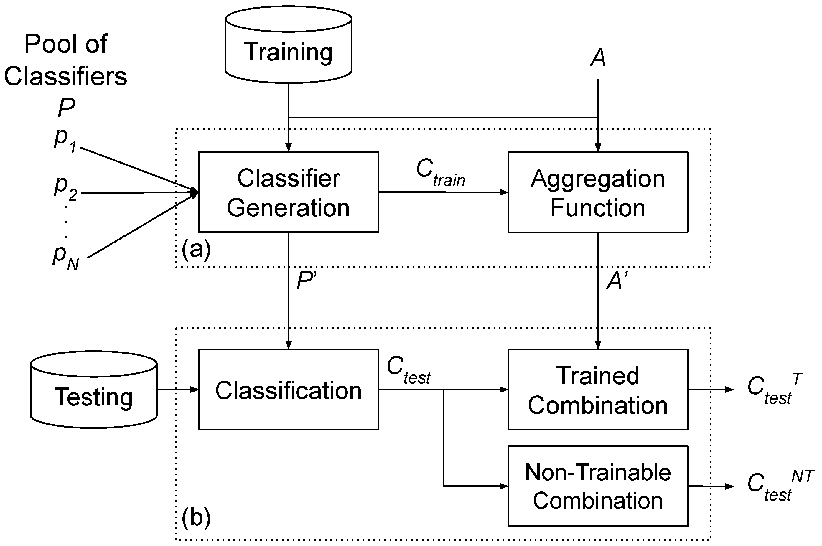
Figure 2.
A general framework of the Multiple Classifier System (MCS), or Ensemble Learning, employing Dynamic Selection (DS). This approach selects one or more models from a Region of Competence (RoC) to classify each pattern of the test set.
Figure 2.
A general framework of the Multiple Classifier System (MCS), or Ensemble Learning, employing Dynamic Selection (DS). This approach selects one or more models from a Region of Competence (RoC) to classify each pattern of the test set.
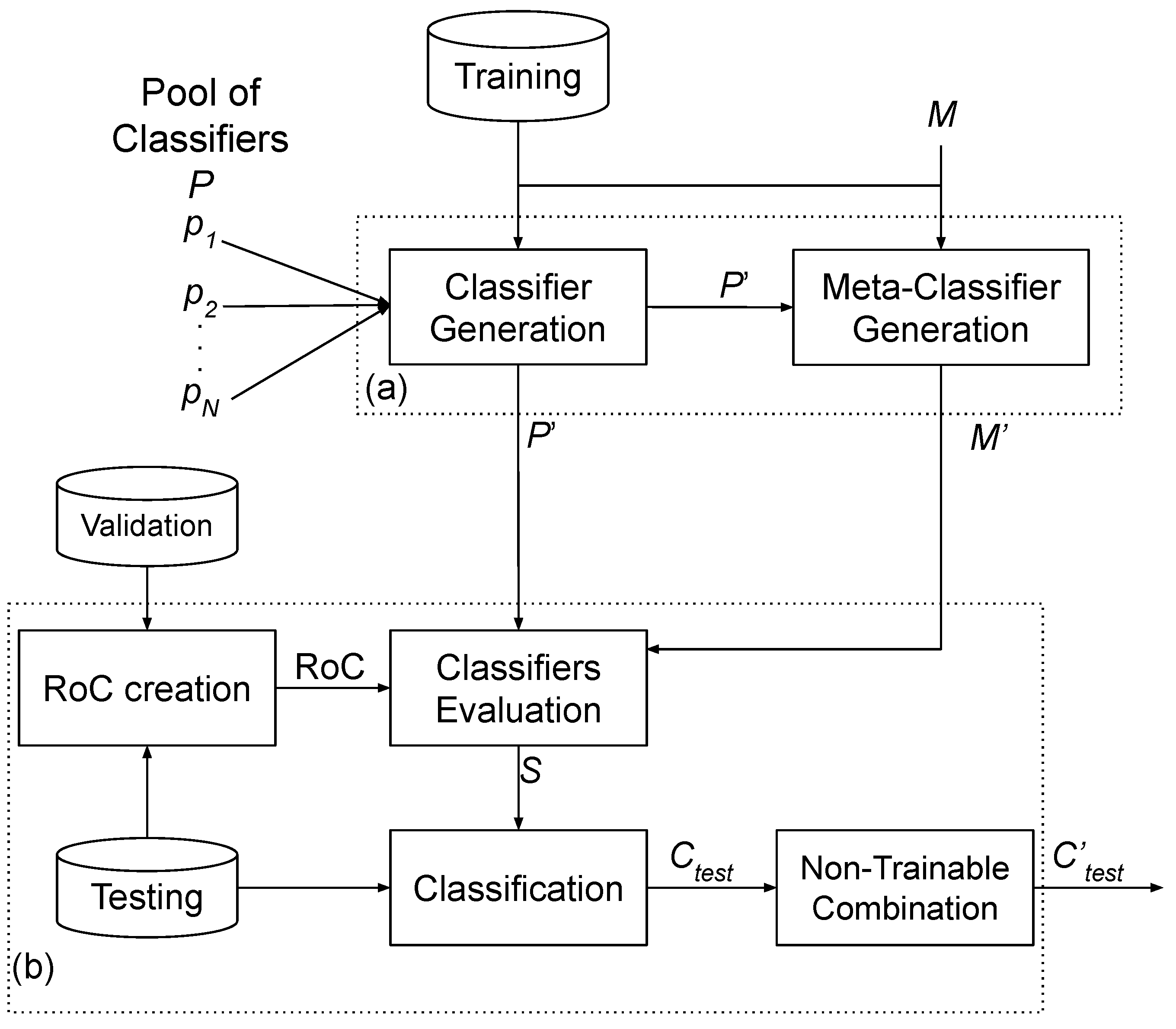
Figure 3.
Accuracy obtained by evaluated single models.
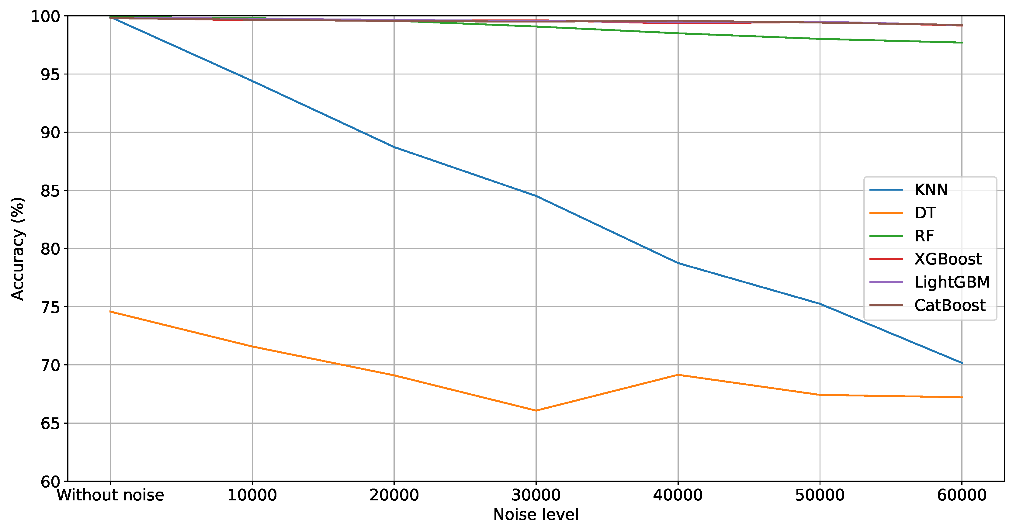
Figure 4.
Accuracy obtained by the evaluated static ensemble models.
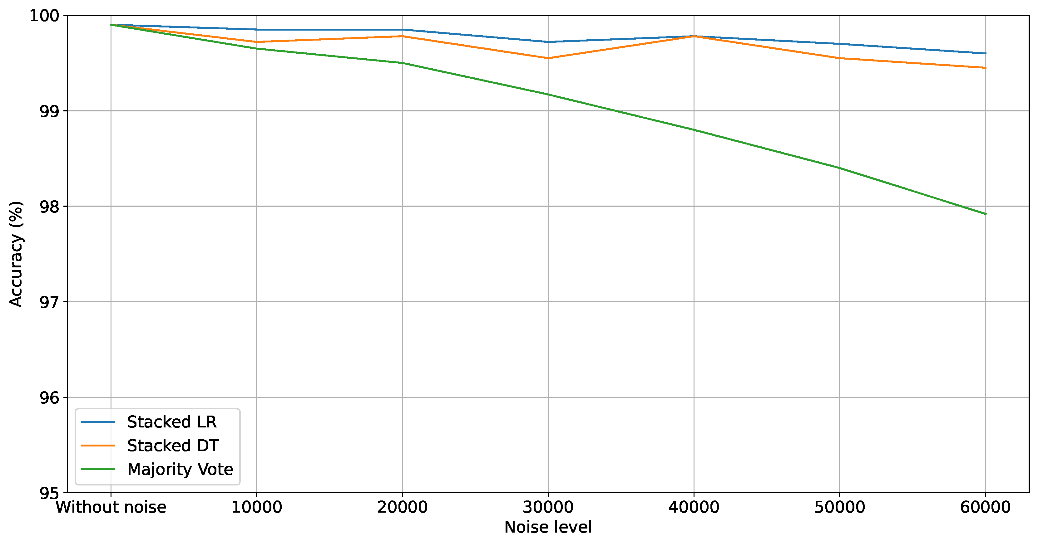
Figure 5.
Accuracy obtained by the evaluated dynamic selection models.
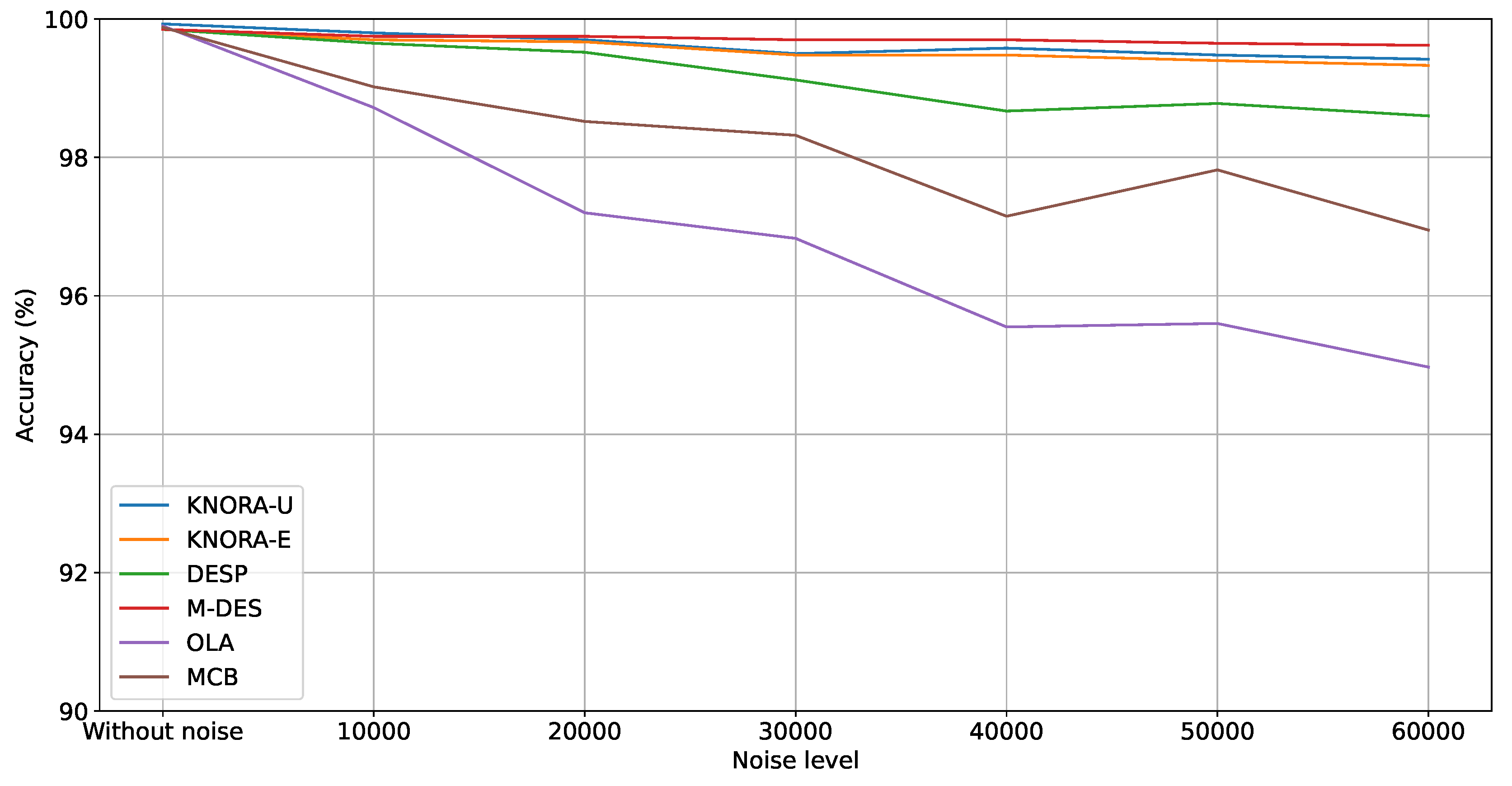
Figure 6.
A, P, and R metrics for the best models of each approach for all noise level scenarios.
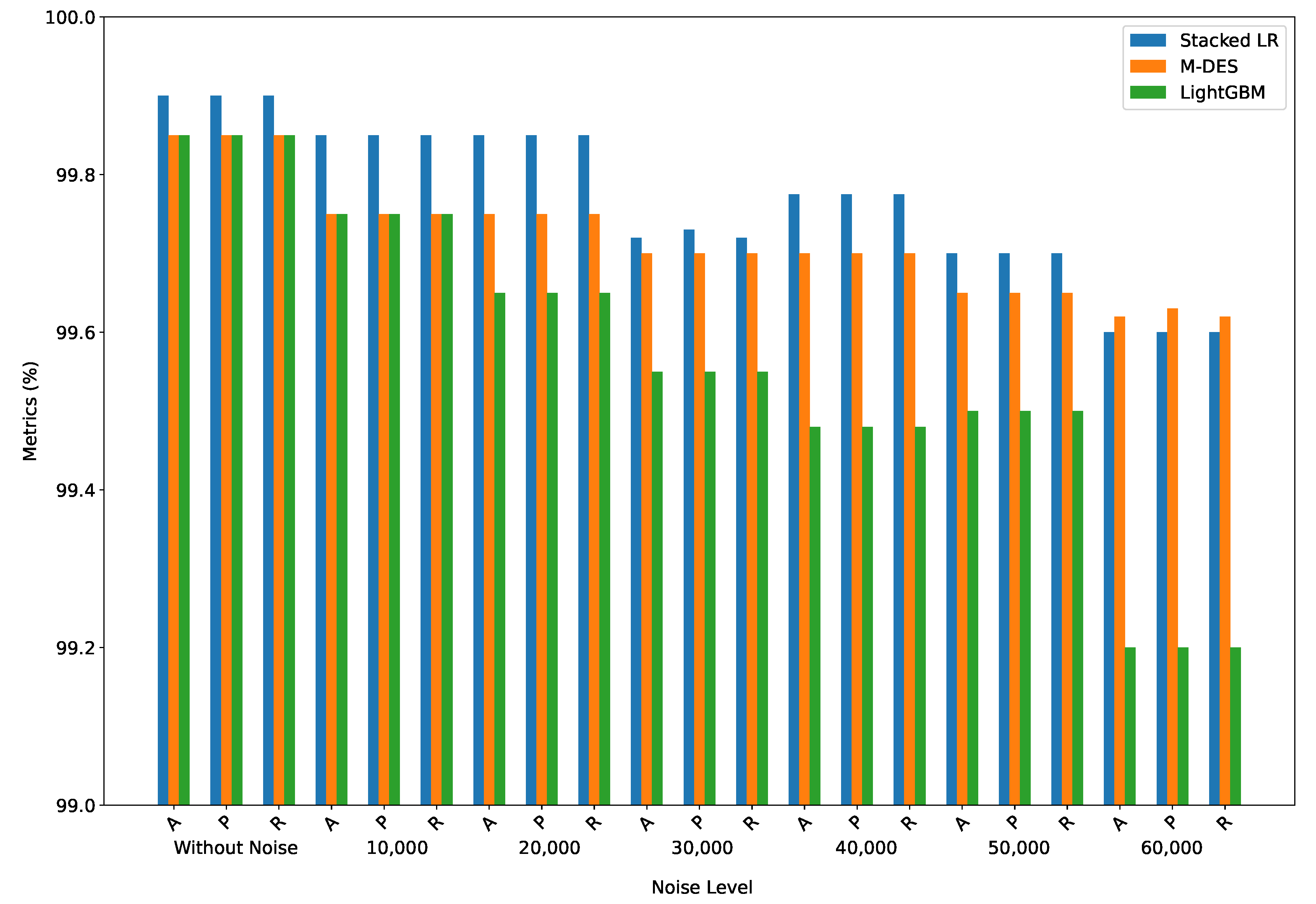
Figure 7.
Accuracy obtained by evaluated single models.
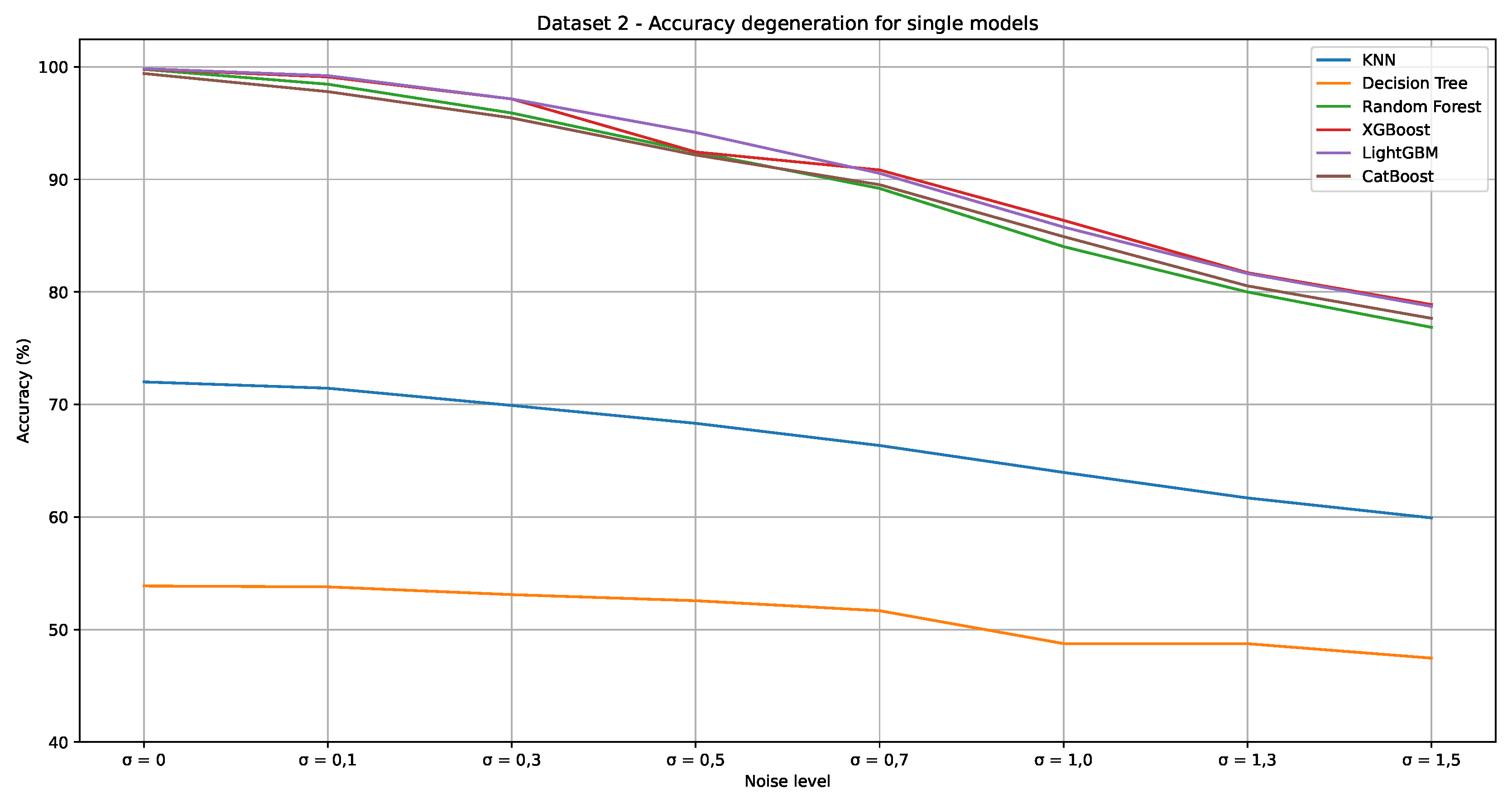
Figure 8.
Accuracy obtained by the evaluated static ensemble models.
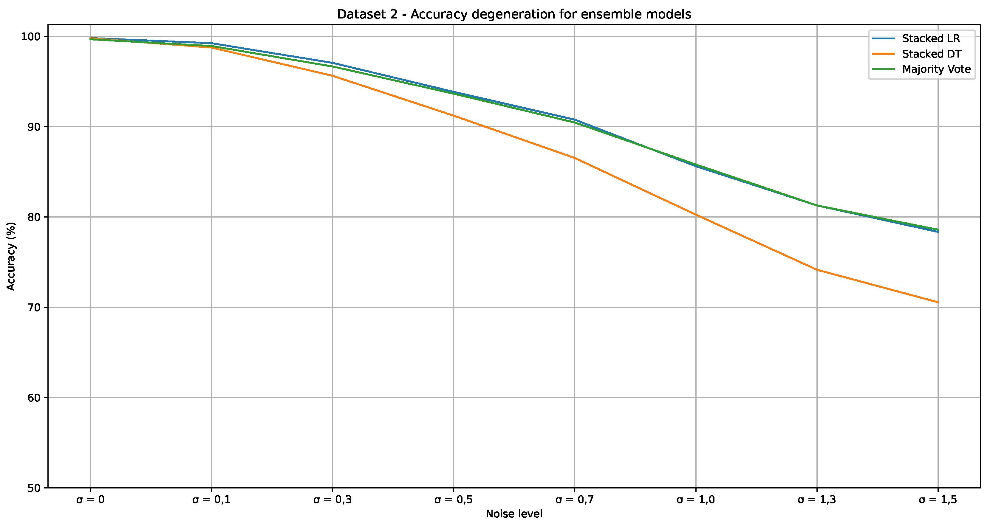
Figure 9.
Accuracy obtained by the evaluated dynamic selection models.
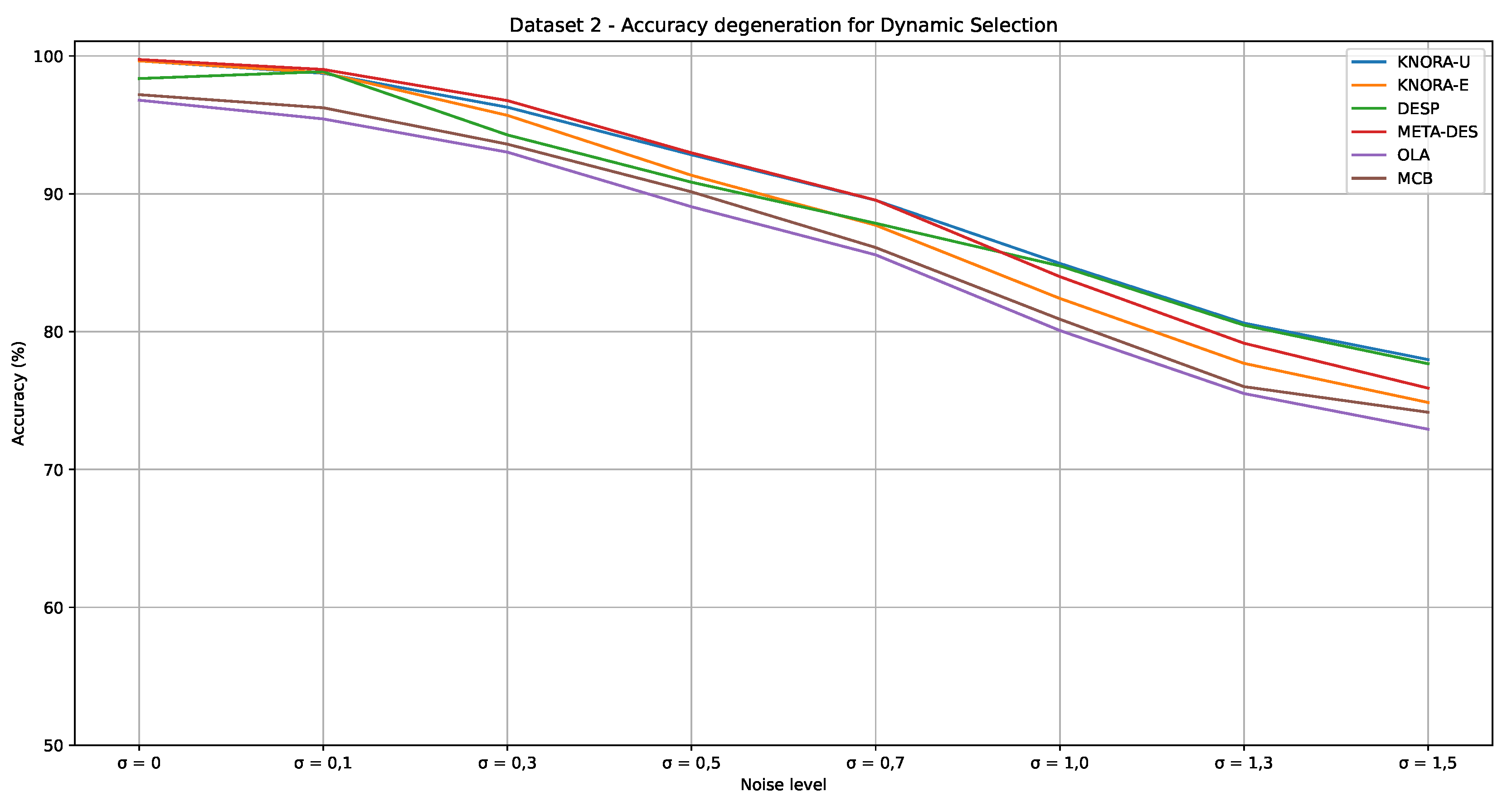
Figure 10.
A, P, and R metrics for the best models of each approach for all noise level scenarios in Dataset 2.
Figure 10.
A, P, and R metrics for the best models of each approach for all noise level scenarios in Dataset 2.
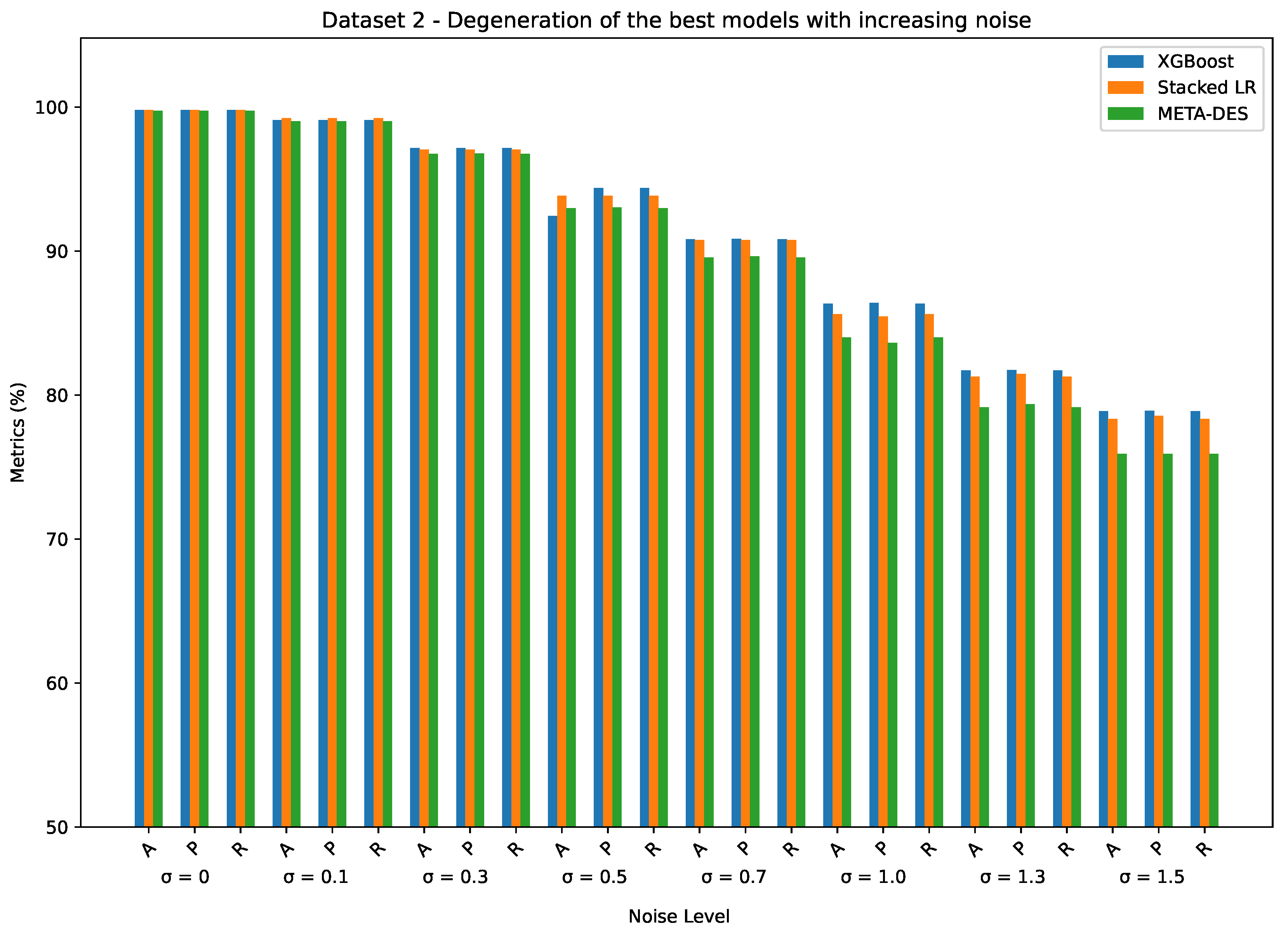

Table 1.
Parameters used for each static ensemble approach.
| Static Ensemble | Parameter | Value |
|---|---|---|
| Majority Vote | voting | {’hard’} |
| Stacked DT | meta_classifier | {DecisionTree} |
| meta_classifier_criterion | {’gini’} | |
| meta_classifier_min_samples_leaf | {1} | |
| meta_classifier_min_samples_split | {2} | |
| meta_classifier_splitter | {’best’} | |
| Stacked LR | meta_classifier | {LogisticRegression} |
Table 2.
Parameters used for each dynamic selection approach.
| Dynamic Selection | Parameter | Value |
|---|---|---|
| DESP | DFP | {False} |
| DESL_perc | {0.5} | |
| IH_rate | {0.3} | |
| k | {7} | |
| knn_classifier | {’knn’} | |
| knn_metric | {’minkowski’} | |
| mode | {’selection’} | |
| KNORA-E KNORA-U |
DFP | {False} |
| DESL_perc | {0.5} | |
| IH_rate | {0.3} | |
| k | {7} | |
| knn_classifier | {’knn’} | |
| knn_metric | {’minkowski’} | |
| MCB | DFP | {False} |
| DESL_perc | {0.5} | |
| IH_rate | {0.3} | |
| diff_thresh | {0.1} | |
| k | {7} | |
| knn_classifier | {’knn’} | |
| knn_metric | {’minkowski’} | |
| knne | {False} | |
| M-DES | DFP | {False} |
| DESL_perc | {0.5} | |
| Hc | {1.0} | |
| IH_rate | {0.3} | |
| Kp | {5} | |
| k | {7} | |
| knn_classifier | {’knn’} | |
| knn_metric | {’minkowski’} | |
| meta_classifier | {’Multinomial naive Bayes’} | |
| mode | {’selection’} | |
| OLA | DFP | {False} |
| DESL_perc | {0.5} | |
| k | {7} | |
| knn_classifier | {’knn’} | |
| knn_metric | {’minkowski’} | |
| knne | {False} |
Table 3.
Hyperparameters used in the grid-search for each model.
| Model | Parameter | Values |
|---|---|---|
| KNN | n_neighbors | {1, 2, 3, 4, 5, 6, 7, 8, 9, 10} |
| weights | {’uniform’, ’distance’} | |
| metric | {’euclidean’, ’manhattan’, ’minkowski’} | |
| Decision Tree | random_state | {0, 1, 2, 42} |
| criterion | {’gini’, ’entropy’} | |
| max_depth | {2, 3, 4, 5, 6, 7, 8, 9, 10, 11} | |
| min_samples_leaf | {1, 2, 4, 6} | |
| Random Forest | n_estimators | {1, 10, 30, 100, 200} |
| random_state | {0, 42} | |
| max_depth | {2, 10, 30, None} | |
| max_features | {’auto’, ’sqrt’, ’log2’} | |
| min_samples_leaf | {1, 2} | |
| XGBoosting | learning_rate | {0.1, 0.547, 0.6427} |
| max_depth | {2, 4, 6, 8, 10} | |
| n_estimators | {2, 4, 8, 10, 200} | |
| min_child_weight | {1, 3, 5} | |
| subsample | {0.7, 0.8, 0.9} | |
| Lgbm | learning_rate | {0.001, 0.01, 0.1} |
| max_depth | {2, 4, 6, 8, 10} | |
| min_child_samples | {20} | |
| n_estimators | {2, 4, 8, 10, 200} | |
| num_leaves | {7, 31} | |
| boosting_type | {’gbdt’, ’goss’} | |
| CatBoosting | learning_rate | {0.1, 0.01, 0.001} |
| max_depth | {2, 4, 6, 8, 10} | |
| n_estimators | {2, 4, 8, 10, 200} |
Table 4.
Metrics for classification evaluation. For all metrics, the higher the value, the better the classification performance.
Table 4.
Metrics for classification evaluation. For all metrics, the higher the value, the better the classification performance.
| Metric | Acronym | Equation | Limits |
|---|---|---|---|
| Accuracy | A | [0, 1] | |
| Precision | P | [0, 1] | |
| Recall | R | [0, 1] |
Table 5.
Evaluation of the single models in Dataset 1 for several noise levels. The best result for each metric is highlighted in bold.
Table 5.
Evaluation of the single models in Dataset 1 for several noise levels. The best result for each metric is highlighted in bold.
| Noise Level | Metric | Single Models | |||||
|---|---|---|---|---|---|---|---|
| CatBoost | DT | KNN | LightGBM | RF | XGBoost | ||
| Without noise | A | 99.80 | 74.58 | 99.90 | 99.85 | 99.90 | 99.83 |
| P | 99.80 | 77.24 | 99.90 | 99.85 | 99.90 | 99.83 | |
| R | 99.80 | 74.58 | 99.90 | 99.85 | 99.90 | 99.83 | |
| 10,000 | A | 99.67 | 71.58 | 94.40 | 99.75 | 99.80 | 99.62 |
| P | 99.67 | 74.52 | 94.36 | 99.75 | 99.80 | 99.63 | |
| R | 99.67 | 71.58 | 94.40 | 99.75 | 99.80 | 99.62 | |
| 20,000 | A | 99.55 | 69.10 | 88.72 | 99.65 | 99.58 | 99.62 |
| P | 99.55 | 72.02 | 88.45 | 99.65 | 99.58 | 99.62 | |
| R | 99.55 | 69.10 | 88.72 | 99.65 | 99.58 | 99.62 | |
| 30,000 | A | 99.50 | 66.07 | 84.52 | 99.55 | 99.08 | 99.62 |
| P | 99.50 | 68.64 | 83.94 | 99.55 | 99.08 | 99.63 | |
| R | 99.50 | 66.07 | 84.52 | 99.55 | 99.08 | 99.62 | |
| 40,000 | A | 99.58 | 69.15 | 78.75 | 99.48 | 98.50 | 99.35 |
| P | 99.58 | 98.50 | 77.58 | 99.48 | 98.50 | 99.35 | |
| R | 99.58 | 98.50 | 78.75 | 99.48 | 98.50 | 99.35 | |
| 50,000 | A | 99.42 | 67.42 | 75.25 | 99.50 | 98.02 | 99.48 |
| P | 99.42 | 67.60 | 73.40 | 99.50 | 98.05 | 99.48 | |
| R | 99.42 | 67.42 | 75.25 | 99.50 | 98.02 | 99.48 | |
| 60,000 | A | 99.22 | 67.22 | 70.17 | 99.20 | 97.70 | 99.17 |
| P | 99.22 | 60.77 | 67.34 | 99.20 | 97.74 | 99.18 | |
| R | 99.22 | 67.22 | 70.17 | 99.20 | 97.70 | 99.17 | |
Table 6.
Evaluation of the static ensemble in Dataset 1 for several noise levels. The best result for each metric is highlighted in bold.
Table 6.
Evaluation of the static ensemble in Dataset 1 for several noise levels. The best result for each metric is highlighted in bold.
| Noise Level | Metric | Static Ensemble | ||
|---|---|---|---|---|
| Majority Vote | Stacked DT | Stacked LR | ||
| Without noise | A | 99.90 | 99.90 | 99.90 |
| P | 99.90 | 99.90 | 99.90 | |
| R | 99.90 | 99.90 | 99.90 | |
| 10,000 | A | 99.65 | 99.72 | 99.85 |
| P | 99.65 | 99.73 | 99.85 | |
| R | 99.65 | 99.72 | 99.85 | |
| 20,000 | A | 99.50 | 99.78 | 99.85 |
| P | 99.50 | 99.78 | 99.85 | |
| R | 99.50 | 99.78 | 99.85 | |
| 30,000 | A | 99.17 | 99.55 | 99.72 |
| P | 99.18 | 99.55 | 99.73 | |
| R | 99.17 | 99.55 | 99.72 | |
| 40,000 | A | 98.80 | 99.78 | 99.78 |
| P | 98.82 | 99.78 | 99.78 | |
| R | 98.80 | 99.78 | 99.78 | |
| 50,000 | A | 98.40 | 99.55 | 99.70 |
| P | 98.44 | 99.55 | 99.70 | |
| R | 98.40 | 99.55 | 99.70 | |
| 60,000 | A | 97.92 | 99.45 | 99.60 |
| P | 98.00 | 99.45 | 99.60 | |
| R | 97.92 | 99.45 | 99.60 | |
Table 7.
Evaluation of the dynamic selection approaches in Dataset 1 for several noise levels. The best result for each metric is highlighted in bold.
Table 7.
Evaluation of the dynamic selection approaches in Dataset 1 for several noise levels. The best result for each metric is highlighted in bold.
| Noise Level | Metric | Dynamic Selection Approach | |||||
|---|---|---|---|---|---|---|---|
| DESP | KNORA-E | KNORA-U | MCB | M-DES | OLA | ||
| Without noise | A | 99.85 | 99.85 | 99.93 | 99.88 | 99.85 | 99.90 |
| P | 99.85 | 99.85 | 99.93 | 99.88 | 99.85 | 99.90 | |
| R | 99.85 | 99.85 | 99.93 | 99.88 | 99.85 | 99.90 | |
| 10,000 | A | 99.65 | 99.70 | 99.80 | 99.98 | 99.75 | 98.72 |
| P | 99.65 | 99.70 | 99.80 | 99.98 | 99.75 | 98.72 | |
| R | 99.65 | 99.70 | 99.80 | 99.98 | 99.75 | 98.72 | |
| 20,000 | A | 99.52 | 99.67 | 99.70 | 98.52 | 99.75 | 97.20 |
| P | 99.53 | 99.68 | 99.70 | 98.53 | 99.75 | 97.26 | |
| R | 99.52 | 99.67 | 99.70 | 98.52 | 99.75 | 97.20 | |
| 30,000 | A | 99.12 | 99.48 | 99.50 | 98.32 | 99.70 | 96.83 |
| P | 99.14 | 99.48 | 99.50 | 98.32 | 99.70 | 96.90 | |
| R | 99.12 | 99.48 | 99.50 | 98.32 | 99.70 | 96.83 | |
| 40,000 | A | 98.67 | 99.48 | 99.58 | 97.15 | 99.70 | 95.55 |
| P | 98.70 | 99.48 | 99.58 | 97.15 | 99.70 | 95.61 | |
| R | 98.67 | 99.48 | 99.58 | 97.15 | 99.70 | 95.55 | |
| 50,000 | A | 98.78 | 99.40 | 99.48 | 97.82 | 99.65 | 95.60 |
| P | 99.79 | 99.40 | 99.48 | 97.82 | 99.65 | 95.64 | |
| R | 99.78 | 99.40 | 99.48 | 97.82 | 99.65 | 95.60 | |
| 60,000 | A | 98.60 | 99.33 | 99.42 | 96.95 | 99.62 | 94.97 |
| P | 98.63 | 99.33 | 99.43 | 96.96 | 99.63 | 95.11 | |
| R | 98.60 | 99.33 | 99.42 | 96.95 | 99.62 | 94.97 | |
Table 8.
Evaluation of the single models in Dataset 2 for several noise levels. The best result for each metric is highlighted in bold.
Table 8.
Evaluation of the single models in Dataset 2 for several noise levels. The best result for each metric is highlighted in bold.
| Noise Level | Metric | Single Models | |||||
|---|---|---|---|---|---|---|---|
| CatBoost | DT | KNN | LightGBM | RF | XGBoost | ||
| Without noise | A | 99.40 | 53.87 | 72.00 | 99.83 | 99.77 | 99.79 |
| P | 99.40 | 43.66 | 71.95 | 99.83 | 99.77 | 99.79 | |
| R | 99.40 | 53.87 | 72.00 | 99.83 | 99.77 | 99.79 | |
| 0.1 | A | 97.79 | 53.79 | 71.44 | 99.21 | 98.45 | 99.10 |
| P | 97.79 | 43.58 | 71.44 | 99.21 | 98.45 | 99.10 | |
| R | 97.79 | 53.79 | 71.44 | 99.21 | 98.45 | 99.10 | |
| 0.3 | A | 95.45 | 53.10 | 69.91 | 97.14 | 95.89 | 97.14 |
| P | 95.45 | 42.84 | 69.84 | 97.14 | 95.89 | 97.14 | |
| R | 95.45 | 53.10 | 69.91 | 97.14 | 95.89 | 97.14 | |
| 0.5 | A | 92.16 | 52.56 | 68.32 | 94.16 | 92.42 | 92.43 |
| P | 92.16 | 48.32 | 68.22 | 94.16 | 92.43 | 94.38 | |
| R | 92.16 | 52.56 | 68.32 | 94.16 | 92.42 | 94.38 | |
| 0.7 | A | 89.52 | 51.67 | 66.35 | 90.53 | 89.19 | 90.83 |
| P | 89.52 | 48.01 | 66.40 | 90.54 | 89.22 | 90.84 | |
| R | 89.52 | 51.67 | 66.35 | 90.53 | 89.19 | 90.83 | |
| 1 | A | 84.91 | 48.75 | 63.96 | 85.76 | 84.02 | 86.35 |
| P | 84.91 | 49.19 | 63.83 | 85.81 | 84.12 | 86.39 | |
| R | 84.91 | 48.75 | 63.96 | 85.76 | 84.02 | 86.35 | |
| 1.3 | A | 80.53 | 48.74 | 61.69 | 81.63 | 79.99 | 81.70 |
| P | 80.53 | 48.98 | 61.53 | 81.68 | 80.06 | 81.73 | |
| R | 80.53 | 48.74 | 61.69 | 81.63 | 79.99 | 81.70 | |
| 1.5 | A | 77.65 | 47.46 | 59.92 | 78.71 | 76.85 | 78.87 |
| P | 77.65 | 46.72 | 59.75 | 78.82 | 76.92 | 78.91 | |
| R | 77.65 | 47.46 | 59.72 | 78.71 | 76.95 | 78.87 | |
Table 9.
Evaluation of the static ensemble in Dataset 2 for several noise levels. The best result for each metric is highlighted in bold.
Table 9.
Evaluation of the static ensemble in Dataset 2 for several noise levels. The best result for each metric is highlighted in bold.
| Noise Level | Metric | Static Ensemble | ||
|---|---|---|---|---|
| Majority Vote | Stacked DT | Stacked LR | ||
| Without noise | A | 99.66 | 99.77 | 99.80 |
| P | 99.66 | 99.77 | 99.80 | |
| R | 99.66 | 99.77 | 99.80 | |
| 0.1 | A | 98.92 | 98.75 | 99.23 |
| P | 98.92 | 98.74 | 99.23 | |
| R | 98.92 | 98.75 | 99.23 | |
| 0.3 | A | 96.65 | 95.62 | 97.05 |
| P | 96.66 | 95.62 | 97.05 | |
| R | 96.65 | 95.62 | 97.05 | |
| 0.5 | A | 93.64 | 91.21 | 93.84 |
| P | 93.67 | 91.21 | 93.84 | |
| R | 93.64 | 91.21 | 93.84 | |
| 0.7 | A | 90.45 | 86.52 | 90.76 |
| P | 90.50 | 86.52 | 90.77 | |
| R | 90.45 | 86.52 | 90.76 | |
| 1 | A | 85.80 | 80.25 | 85.61 |
| P | 85.95 | 80.10 | 85.45 | |
| R | 85.80 | 80.25 | 85.61 | |
| 1.3 | A | 81.27 | 74.15 | 81.27 |
| P | 81.41 | 74.35 | 81.47 | |
| R | 81.27 | 74.15 | 81.27 | |
| 1.5 | A | 78.58 | 70.55 | 78.34 |
| P | 78.74 | 71.05 | 78.56 | |
| R | 78.58 | 70.55 | 78.34 | |
Table 10.
Evaluation of the dynamic selection approaches in Dataset 2 for several noise levels. The best result for each metric is highlighted in bold.
Table 10.
Evaluation of the dynamic selection approaches in Dataset 2 for several noise levels. The best result for each metric is highlighted in bold.
| Noise Level | Metric | Dynamic Selection Approach | |||||
|---|---|---|---|---|---|---|---|
| DESP | KNORA-E | KNORA-U | MCB | M-DES | OLA | ||
| Without noise | A | 98.36 | 99.64 | 99.64 | 97.19 | 99.74 | 96.79 |
| P | 98.36 | 99.64 | 99.64 | 97.19 | 99.74 | 96.79 | |
| R | 98.36 | 99.64 | 99.64 | 97.19 | 99.74 | 96.79 | |
| 0.1 | A | 98.86 | 98.79 | 98.74 | 96.24 | 99.02 | 95.43 |
| P | 98.96 | 98.79 | 98.74 | 96.25 | 99.02 | 95.43 | |
| R | 98.86 | 98.79 | 98.74 | 96.24 | 99.02 | 95.43 | |
| 0.3 | A | 94.27 | 95.69 | 96.28 | 93.60 | 96.76 | 93.02 |
| P | 94.41 | 95.71 | 96.30 | 93.62 | 96.77 | 93.02 | |
| R | 94.27 | 95.69 | 96.28 | 93.60 | 96.76 | 93.02 | |
| 0.5 | A | 90.84 | 91.34 | 92.83 | 90.14 | 92.97 | 89.06 |
| P | 91.87 | 91.40 | 92.89 | 90.19 | 93.02 | 89.09 | |
| R | 90.84 | 91.34 | 92.83 | 90.14 | 92.97 | 89.06 | |
| 0.7 | A | 87.86 | 87.72 | 89.53 | 86.10 | 89.54 | 85.57 |
| P | 88.10 | 87.80 | 89.61 | 86.15 | 89.62 | 85.61 | |
| R | 87.86 | 87.72 | 89.53 | 86.10 | 89.54 | 85.57 | |
| 1 | A | 84.77 | 82.41 | 84.95 | 80.90 | 83.99 | 80.08 |
| P | 84.30 | 82.25 | 84.19 | 79.91 | 83.61 | 80.00 | |
| R | 84.77 | 82.41 | 84.19 | 80.90 | 83.99 | 80.08 | |
| 1.3 | A | 80.47 | 77.70 | 80.62 | 76.01 | 79.16 | 75.51 |
| P | 80.67 | 77.90 | 80.92 | 76.20 | 79.35 | 75.71 | |
| R | 80.47 | 77.70 | 80.62 | 76.01 | 79.16 | 75.51 | |
| 1.5 | A | 77.67 | 74.86 | 77.97 | 74.15 | 75.90 | 72.92 |
| P | 77.87 | 74.98 | 78.05 | 74.35 | 75.90 | 72.98 | |
| R | 77.67 | 74.86 | 77.97 | 74.15 | 75.90 | 72.92 | |
Disclaimer/Publisher’s Note: The statements, opinions and data contained in all publications are solely those of the individual author(s) and contributor(s) and not of MDPI and/or the editor(s). MDPI and/or the editor(s) disclaim responsibility for any injury to people or property resulting from any ideas, methods, instructions or products referred to in the content. |
© 2024 by the authors. Licensee MDPI, Basel, Switzerland. This article is an open access article distributed under the terms and conditions of the Creative Commons Attribution (CC BY) license (http://creativecommons.org/licenses/by/4.0/).
Copyright: This open access article is published under a Creative Commons CC BY 4.0 license, which permit the free download, distribution, and reuse, provided that the author and preprint are cited in any reuse.


