
Submitted:
23 September 2024
Posted:
23 September 2024
You are already at the latest version
Abstract
Structural Health Monitoring (SHM) plays a vital role in ensuring the health status of a wide range of structures, such as bridges, buildings and large infrastructure in general. The advantages of this process can be further enhanced by incorporating more numerical and statistical approaches into traditional methods, such as Finite Element Analysis and Machine Learning. In this study a bridge structure is examined, and neural networks are trained with data derived from finite element analyses under static loads and dynamic excitations. Initially, a binary classification problem is addressed, where numerically trained classifiers are tasked with identifying whether the structure is in a healthy state or not. This category is further divided into two subcategories, depending on the extent of the damage present in the structure. Subsequently, a multi-class classification problem is defined, where three different damage classes of the same extent are considered, and the trained network is required to distinguish between them. Finally, conclusions are drawn from the results of the study regarding the model error parameter, the impact of the damage size, as well as the types of neural networks and training data used.
Keywords:
Structural Health Monitoring (SHM)
; FEM
; Machine Learning (ML)
; Artificial Neural Networks (ANNs)
; Deep Neural Networks (DNNs)
; Convolutional Neural Networks (CNNs)
1. Introduction
In the modern world we live in, as it has evolved, we observe all around us a wide range of engineering structures, from simple to extremely complex and intricate, serving various purposes. When it comes to large-scale structures such as bridges, buildings, and infrastructure, a critical field of engineering closely tied to these is Structural Health Monitoring (SHM) [1],[2]. For mechanical systems with rotating components, this field is referred to as Condition Monitoring (CM). Both SHM and CM utilize engineering analysis methodologies that enable the assessment of the health status of the aforementioned structures and mechanical systems. Essentially, these methodologies are divided into two major stages. In the first stage, the necessary data regarding the structure's response over a given period of time must be acquired, and in the second stage, the data is analyzed to draw conclusions about the presence and severity of potential damage in the structure.
The most important part of the SHM process is the acquisition or generation of the required data, as the subsequent steps depend on it [3]. Data acquisition can be done in two ways. The first way is the traditional method, where data is obtained through experimental measurements conducted on the physical structure or on a test model. The second method involves the use of computational and numerical techniques, such as the Finite Element Method (FEM). Finite element models can be optimized through a process called Model Updating [4], which uses experimental data from the actual structure to ensure that the model behaves as closely as possible to reality. This allows for a wide range of analyses to be conducted, simulating various loading conditions and uncertainties in a cost-effective and time-efficient manner. Once the necessary data has been collected, the second stage in the damage detection process involves the appropriate processing and analysis of this data to detect, any patterns that deviate from the healthy state, and anomalies. Various techniques are used for this purpose, such as signal analysis, statistical analysis, and Machine Learning (ML) models. Through the use of Artificial Neural Network (ANN) models, numerical classifiers are implemented, which are ideal for detecting damage and, therefore, for addressing the problem of SHM [5],[6] .
Outline of This Paper
This paper begins with the presentation of the structure and the description of the process followed. The simple model and the actual model are defined, both referring to finite element models used to generate the training and validation data for the neural networks, respectively. Next, the training of the Neural Networks is conducted, first addressing the Binary Classification Problem, followed by the Multi-Class Classification Problem. Finally, the results of the Neural Network predictions are presented, and conclusions are drawn regarding critical parameters that play a decisive role in their final performance.
2. Methodology
2.1. Geometry and Materials
In the present work, the mechanical structure under examination is a footbridge, whose basic views, main dimensions, as well as certain design details, are presented in Figure 1. This bridge is a space truss whose members have a hollow geometry and are connected at their ends using spherical joint connections. Its total length is 10 meters, with a width and height of 2 meters. The material chosen for the structure is a common steel with an elastic modulus of E = 210 GPa and a density of ρ = 7850 kg/m³.
2.2. Description of the Process
Initially, for the geometry of the bridge presented earlier, a suitable Finite Element (FE) algorithm is created in MATLAB, where the structure is simulated using one-dimensional rod elements (1D Rod Elements). Based on this modeling, the training data for the Neural Networks will be generated. Since we do not have an experimental setup available to evaluate the effectiveness of the trained Neural Networks, the experimental setup is substituted with simulations, which are conducted using commercial FE software. Two-dimensional shell elements (2D Shell Elements) are chosen to model the experimental setup, rather than the one-dimensional elements used in the MATLAB model. This choice will affect the prediction accuracy results of the trained Neural Networks (model error parameter). From this point forward, when referring to the “simple” model, the bridge model simulated in MATLAB with the one-dimensional rod elements is considered, whereas the “actual” model refers to the modeling done in the commercial software, which serves as the experimental setup.
In the Machine Learning part, two types of problems are addressed. The first is the Binary Classification Problem, where two health states of the structure are defined (healthy or damaged), and the trained networks are tasked with determining the necessary "decision boundary" between them. Similarly, the Multi-Class Classification Problem is addressed, where three different damage classes of the same extent are defined, and the trained networks are required to identify and classify these distinct damage states. For both types of problems, Neural Networks are trained using data from static analyses, as well as Neural Networks trained with data from dynamic analyses. In the case of the “statically” trained Neural Networks, their architecture follows the structure of Deep Neural Networks (DNNs), utilizing fully connected layers. On the other hand, “dynamically” trained networks employ the structure of Convolutional Neural Networks (CNNs), leveraging convolutional layers to extract information from the time-dependent data. This distinction allows the networks to process the different types of input data more effectively, enhancing their ability to classify the structural health conditions in both static and dynamic contexts.
3.“. Simple” and “Actual” Models
3.1“. Simple” Model Implementation
The “simple” model refers to the simplified modeling using FE codes implemented in MATLAB, based on which the necessary static and dynamic analyses will be conducted and the training data for the Neural Networks will be derived. The above bridge we are tasked with modeling, forms a space truss. A truss is created by joining straight members at nodes, which are located at the ends of each member. The individual members of the space truss are two-force members, meaning they are subjected to two equal and opposite forces directed along their axis. Therefore, each member is subjected only to axial loading. As a result, for this simplified modeling of the structure, 1D axial rod elements were chosen for use.
The modeling of the structure begins with the appropriate numbering and naming of the members and nodes, respectively, as shown in Figure 2. This information must be arranged in a suitable format to be easily manageable by the FE codes that will be performed. Thus, two text files are created, containing information concerning the numbering and spatial arrangement of the nodes, as well as the connectivity between the members and nodes.
Regarding the boundary conditions, the bridge is supported at nodes A, F, L, and Q, where their degrees of freedom along the X, Y, and Z axes are constrained. Restricting rotation around the three axes is unnecessary, as the structure is a space truss modeled with axial rod elements, meaning its members cannot resist bending and torsional moments. It is important to emphasize that the displacements of all nodes in the Y direction are restricted. This is necessary because, without these constraints, the model would be statically indeterminate.
3.1.1. Algorithm for Training Data Generation Using Static Analyses
The algorithm presented in Figure 3 below, forms the basis for generating the training data from static analyses, which are used in the respective Neural Networks for their training and will be presented in the following sections. This algorithm defines a general code structure to be followed, where in each case the health state of the structure must be appropriately defined, as well as the labels that describe it.
In each analysis, two random nodes are selected, where forces are applied in the X and Z directions, with random magnitudes. Obviously, in any given analysis, the two selected nodes cannot be the same, and no forces are applied to the fixed supports.
The normalization of the displacement results is achieved by dividing, in each individual analysis, the displacement values of all nodes (in the X and Z directions) by the maximum absolute displacement value observed at one of them. Similarly, the stresses of all members are normalized relative to the maximum absolute stress observed in one of them. This ensures that all stress and displacement values fall within a range of -1 to 1.
After the above algorithm is executed, the normalized results of the analyses are obtained in the form shown in Figure 4 and are saved in a .csv file.
3.1.2. Algorithm for Training Data Generation Using Dynamic Analyses
In Figure 5 below, the structure of the algorithm is presented used to extract all the training data for Neural Networks trained with data from dynamic analyses.
In contrast to the static problem presented earlier (where loads were applied to randomly selected nodes in each analysis), in the case of the dynamic problem, two nodes are consistently selected to apply the excitations. Specifically, these nodes are Node C and Node O. Excitations are applied in both directions (X and Z) for both nodes, respectively. Figure 6a below schematically illustrates the excitations.
These excitations are defined as the sum of harmonic excitations and are given by the following expressions:
Where: A1 to A10 are random excitation amplitudes, and ω1 to ω10 the first ten natural frequencies of the structure derived from the FE software
As "sensors," the degrees of freedom of the nodes for which the displacement time histories will be recorded in each analysis are defined. Six nodes of the structure are selected: B, D, G, N, R, and U. This results in a total of 12 channels (2 sensors for each node, corresponding to the X and Z directions), from which the response of the structure will be measured. For each channel, a matrix is created with n rows and t columns (3500 timesteps, 3.5 seconds total simulation time), where each row stores the response from a particular analysis. Once all analyses are completed, the response values in each matrix are normalized by the maximum absolute value recorded in each channel. This results in 12 normalized matrices containing the sensor responses from the n analyses. This separation of results into individual channels (Figure 7) is essential because the data is intended for training one-dimensional convolutional neural networks (1D CNNs), which require this format for input data
3.2“. Actual” Model Implementation
After the necessary training of the Neural Networks, we are required to validate their effectiveness using data ideally derived from the actual structure or from an experimental setup. Since we do not have access to either of these setups, the structure is simulated using commercial FE software, utilizing 2D shell elements (Figure 8). This approach provides the model with greater realism compared to the “simple” model, as shell elements can handle not only axial loads but also transverse, bending, and torsional. Additionally, the bridge members have a hollow beam geometry with a relatively small thickness compared to the other two dimensions, making shell elements suitable for their description.
To describe the connections between the structural members of the bridge (modelling of the spherical joint connections), Rigid Body Elements were used. These elements are connected to the members in the manner depicted in Figure 9a below. Subsequently, the appropriate boundary conditions are applied (Figure 9b). As explained earlier in the “simple” model, nodes A, F, L, and Q are fixed (all six degrees of freedom are constrained here), and the displacements of all nodes in the Y direction are restricted (to maintain consistency with the “simple” model).
Once the necessary procedure for creating the "actual" FE model of the structure is completed, the required static and dynamic analyses can be conducted. The results of these analyses will be used to evaluate the effectiveness of the trained Neural Networks. The outcomes from both the static and dynamic analyses are normalized and appropriately arranged with their respective labels to ensure full consistency with the corresponding data obtained from the analyses of the "simple" model.
4. Binary Classification Problem
The term "Binary Classification Problem" refers to training a Neural Network to recognize patterns and trends in data, with the aim of categorizing the input into two classes (the structure is either healthy or damaged). In this section, Neural Networks will be trained using both static and dynamic data, enabling them to identify whether the bridge exhibits damage or remains in a healthy state.
This section is divided into two main subsections, with the key distinction being the severity of the damage in the structure. Section 4.1 focuses on Neural Networks trained with data where the structure is either healthy or has a "minor" damage, while in Section 4.2, the networks are trained similarly, but the damage is considered "extensive" in the damaged case.
4.1. Training of ANNs for Minor Damage Detection
As a "minor" damage scenario, we define a 90% reduction in the material's modulus of elasticity for a randomly selected member. In each analysis of the bridge in a non-healthy state, one member is randomly chosen, and its modulus of elasticity is reduced by 90%.
In the Table 1 below, key information is provided regarding the training of two Neural Networks using data from static and dynamic analyses, respectively, for the detection of "minor" damage in the structure.
4.2. Training of ANNs for Extensive Damage Detection
In the case of “extensive” damage, we assume that in the non-healthy state of the bridge, there are four beams with a reduced modulus of elasticity by 90%. Therefore, in each analysis concerning a damaged state of the bridge, four beams are randomly selected and are assigned a modulus of elasticity equal to 21 GPa.
Table 2 provides information regarding the training of two neural networks, with data derived from static and dynamic analyses, concerning the diagnosis of significant damage in the structure.
5. Multi-Class Classification Problem
The “Multi-Class Classification Problem” involves training of two Neural Networks utilizing response data from static and dynamic analyses, respectively, which will be capable of recognizing and carrying out predictions for three different damage class scenarios in the bridge.
The three damage classes (Figure 14) that can occur in the bridge are defined as follows:
- Class 1: Members 11 and 43 (numbered according to Figure 2) have a 90% reduction in their modulus of elasticity.
- Class 2: Members 40 and 41 have a 90% reduction in their modulus of elasticity.
- Class 3: Members 17 and 18 have a 90% reduction in their modulus of elasticity.
Table 3 below provides the necessary information regarding the training of the two Neural Networks.
6. Results – Testing of the Trained Neural Networks
In this section, the effectiveness of the trained Neural Networks will be evaluated based on the corresponding data derived from static and dynamic analyses of the “actual” FE model of the structure. Subsequently, the results obtained are discussed.
6.1.“. Binary Classification Problem” – Neural Networks Testing
For the evaluation of each Neural Network model trained for the binary classification task, 10 analyses are conducted where the structure is in a healthy state and 10 where the structure is damaged (static or dynamic analyses, depending on the network for which they are intended). The results of these 20 analyses are fed into the Neural Networks, and the success of their predictions is assessed. Figure 17 presents the confusion matrices that demonstrate the prediction results.
Below, in Table 4, the prediction results of the neural networks are compiled.
From the above results, it can be observed that when comparing the Neural Networks trained with data from static analyses (DNNs), the network tasked with recognizing larger damages achieves a better prediction rate compared to the one for smaller damages, i.e., 75% versus 55%. The same trend is evident among the networks trained with dynamic analysis data (CNNs), where the success rates are 90% for large damage and 80% for smaller, respectively.
Therefore, in all cases, regardless of the type of network or the data used for its training, it is easier for a network to recognize a larger damage compared to a smaller one. This is easily explained and understood, as each Neural Network attempts to adjust its weights appropriately to find the suitable correlations that will lead to the correct separation between the two classes (healthy or damaged). Consequently, if the differences in the input data between classes 1 and 2 are very small (e.g., in the case of minor damage), the network will struggle to find the appropriate "borderline" between them. In contrast, with larger damage, the data become more distinct and clearer (showing more pronounced differences between the data of the two classes), making it easier to identify the features that distinguish it from the healthy state.
6.2.“. Multi-Class Classification Problem” – Neural Networks Testing
Similarly to the Binary Classification Problem, for each of the 3 damage classes, 10 analyses are conducted based on the “actual” FE model of the structure. Therefore, a total of 30 analyses are generated (either static or dynamic, depending on the network for which they are intended), upon which the performance of the Neural Networks' predictions is evaluated.
Below, in Figure 18 and Figure 19, the confusion matrices and the histograms of the prediction results are presented, respectively.
The trained network, Multiclass_static_DNN, achieves an overall prediction accuracy of 66.7%. This percentage does not represent α good predictive performance, especially considering that during the validation phase, the network achieved an accuracy of 98.33%. This indicates a poor correlation between the training data and the test data (high model error), meaning that the network does not generalize well.
We also observe, from both the bar charts and the confusion matrix data, that the network tends to predict two of the three classes with greater accuracy. Specifically, 90% of the data from class 3 and 80% from class 2 were predicted correctly. On the other hand, only 30% of the data from class 1 were accurately predicted. This reveals a clear "preference" of the network for distinguishing and recognizing classes 2 and 3 to a greater extent.
Similarly, the overall prediction accuracy of the trained network Multiclass_dynamic_CNN reaches 70%. Compared to the previous network, this one achieves relatively better performance. We observe that class 2 is predicted with 100% accuracy, while class 3 is predicted with 70% and class 1 with 40%. Thus, in this case as well, the Neural Network shows a tendency to confuse class 1.
This tendency exhibited by both Neural Networks, in their inability to recognize the class 1 damage, is not random. If we refer to Figure 14 and examine how the damage classes are defined, we will see that both class 2 and class 3 are defined in such a way that the damaged members are adjacent and share a common node. In contrast, damage class 1 refers to two members that are on different planes (parallel planes), meaning they are not adjacent and do not share a common node. As a result, classes 2 and 3 are more easily detected by the network because larger displacements occur at the common node where their members are connected. In other words, class 1 could be considered as a class of "smaller" damage, due to its lesser impact on the displacements of the involved nodes, making it harder for the network to detect.
7. Discussion
The training and the effectiveness of a Neural Network in recognizing or detecting damage in structures, or more generally in mechanical engineering applications, is a problem influenced by many factors that clearly affect the performance and accuracy of the final predictions. Based on the analyses from the previous sections, certain conclusions were drawn regarding critical parameters that play a decisive role in the final performance of a network, which are outlined below.
- Model Error Parameter
In general, the prediction performance of the trained neural networks was not as desired. This is primarily due to the model error that exists between the “simple” and the “actual” models. It was observed that, while the accuracy of the networks' predictions during training (on the validation dataset, consisting of data the network had not "seen" before, but coming from the same set as the training data) was above 96%, when they were fed with data from the real model's analyses, the prediction rates were significantly lower. This indicates that the correlation between the training and test data is not satisfactory, despite the normalization of the data, which was an attempt to reduce, to some extent, the differences in the absolute values of the responses between the two models.
Thus, for the proper training and testing of Neural Networks, there needs to be as little model error as possible between the model used for generating training data and the real structure (this can be achieved by implementing model updating FE methods). This would maximize prediction performance and ensure greater reliability in the evaluation process.
- Extent of the Damage
Regarding the size of the damage in the structure, the results of the Neural Networks evaluated in Section 6 revealed a clear trend. Specifically, in all cases, regardless of the type of network or the data used for training, it is easier for a network to recognize a larger damage compared to a smaller one. This can be explained and understood as the Neural Network adjusts its weights to find the correct correlations that allow for the proper separation between the two classes (healthy or damaged). When the differences in the input data between classes 1 and 2 are very small (as in the case of minor damage), the network struggles to find the appropriate "boundary" between them. On the other hand, in the case of more significant damage, the data become more distinct and clearer, making it easier to separate the features that differentiate it from the healthy state.
- Type of the Neural Network and Training Data
Among the Neural Networks trained in all cases, the Convolutional Neural Networks (CNNs) used for dynamic analyses achieved higher prediction performance compared to the corresponding Deep Neural Networks (DNNs) used for static analyses. This could be attributed to two main factors: the type of data used for training and the structure of the Neural Network itself.
Regarding the type of data, it is evident that dynamic analysis responses contain more information compared to static responses. Dynamic analyses provide insights into the inherent characteristics of the structure, such as natural frequencies, mode shapes, and damping properties. In contrast, static analyses yield constant and absolute values for displacements, stresses, and strains, which offer less additional information. However, a drawback of dynamic analyses is the longer time required to perform them, compared to static analyses. This is one of the primary reasons, why training neural networks with static analysis data is also considered in this work.
Concerning the structure of the Neural Network, CNNs appear to outperform standard DNNs. CNNs incorporate convolutional layers in their architecture, which are capable of "scanning" the information and extracting useful features before proceeding to the fully connected layers. This gives CNNs the advantage of filtering the data and retaining only the useful information that aids in categorizing the different classes.
Author Contributions
Conceptualization, A.A; Methodology, A.K and P.S and A.A; Software, A.K and P.S.; Validation, A.K and A.A.; Formal Analysis, A.K.; Investigation, A.K. and A.A.; Resources, A.K. and P.S.; Data curation, A.K. and P.S. and A.A.; Writing-original draft preparation, A.K.; Writing-review and editing A.A.; Visualization, A.K. and P.S. and A.A.; Supervision, A.A. All authors have read and agreed to the published version of the manuscript.
Funding
Not applicable.
Data Availability Statement
Not applicable.
Acknowledgments
Not applicable.
Conflicts of Interest
The authors declare no conflicts of interest.
References
- Döhler, M.; Hille, F.; Mevel, L.; Rücker, W. Structural health monitoring with statistical methods during progressive damage test of S101 Bridge. Engineering Structures 2014, 69, 183–193. [Google Scholar] [CrossRef]
- Sousa Tomé, E.; Pimentel, M.; Figueiras, J. Damage detection under environmental and operational effects using cointegration analysis – Application to experimental data from a cable-stayed bridge. Mechanical Systems and Signal Processing 2020, 135, 106386. [Google Scholar] [CrossRef]
- Seventekidis, P.; Giagopoulos, D.; Arailopoulos, A.; Markogiannaki, O. Structural Health Monitoring using deep learning with optimal finite element model generated data. Mechanical Systems and Signal Processing 2020, 145, 106972. [Google Scholar] [CrossRef]
- Giagopoulos, D.; Arailopoulos, A. Computational framework for model updating of large scale linear and nonlinear finite element models using state of the art evolution strategy. Computers & Structures 2017, 192, 210–232. [Google Scholar] [CrossRef]
- Zhao, R.; Yan, R.; Chen, Z.; Mao, K.; Wang, P.; Gao, R.X. Deep learning and its applications to machine health monitoring. Mechanical Systems and Signal Processing 2019, 115, 213–237. [Google Scholar] [CrossRef]
- Yu, Y.; Wang, C.; Gu, X.; Li, J. A novel deep learning-based method for damage identification of smart building structures. Structural Health Monitoring 2018, 18, 143–163. [Google Scholar] [CrossRef]
Figure 1.
Bridge structure. (a) Isometric view. (b) Front view. (c) Spherical joint connection detail. (d) Detail of a member’s cross-section. .
Figure 1.
Bridge structure. (a) Isometric view. (b) Front view. (c) Spherical joint connection detail. (d) Detail of a member’s cross-section. .
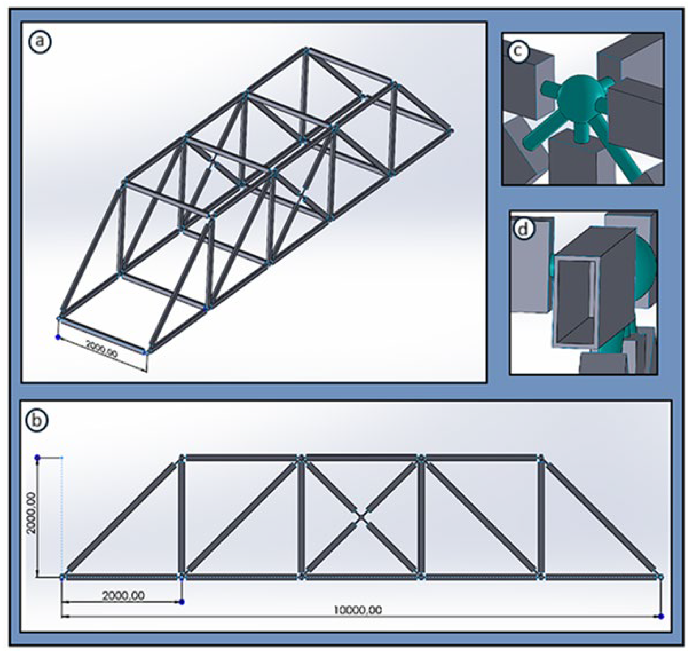
Figure 2.
Naming and numbering of the structure’s nodes and members.
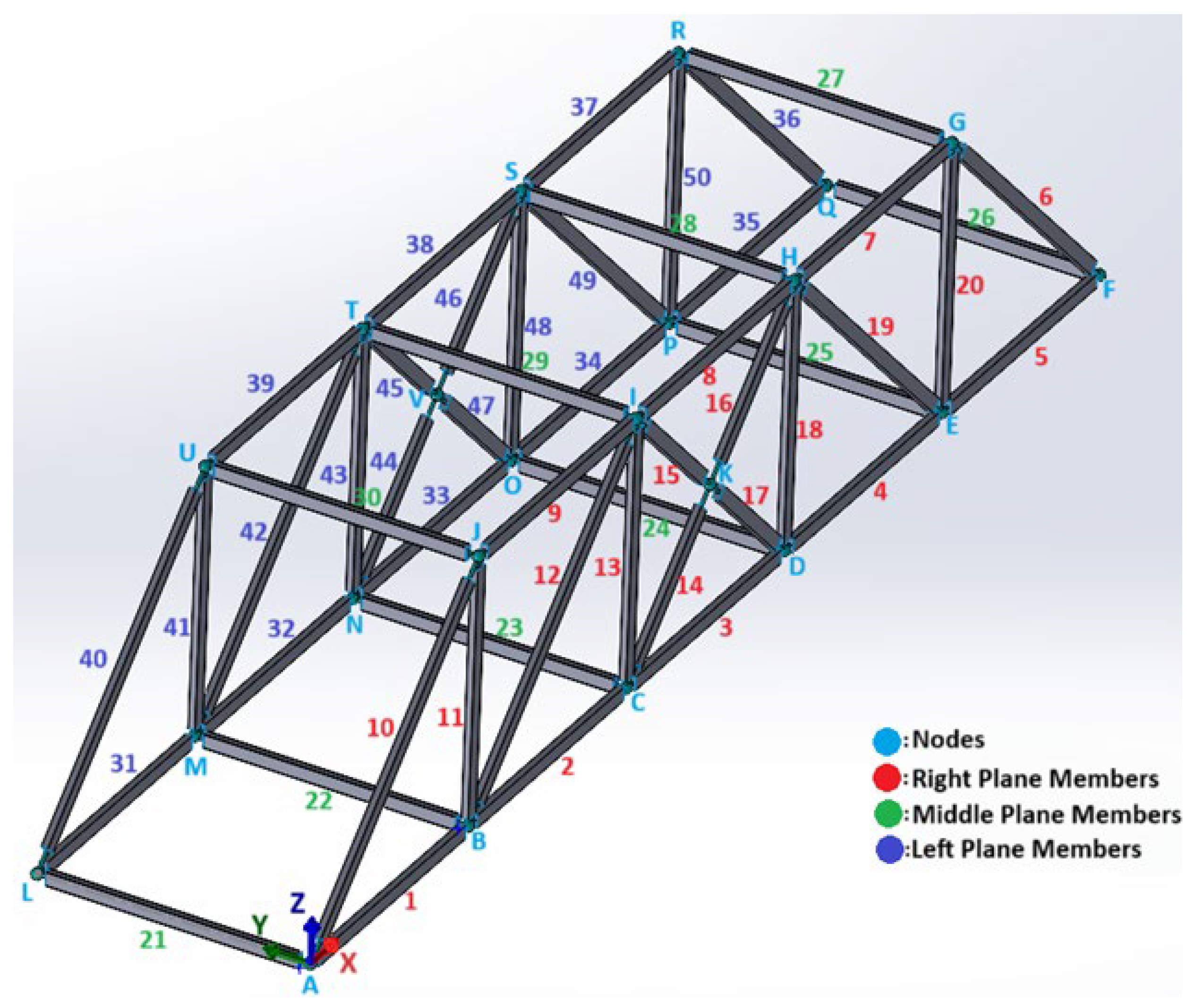
Figure 3.
Algorithm 1.
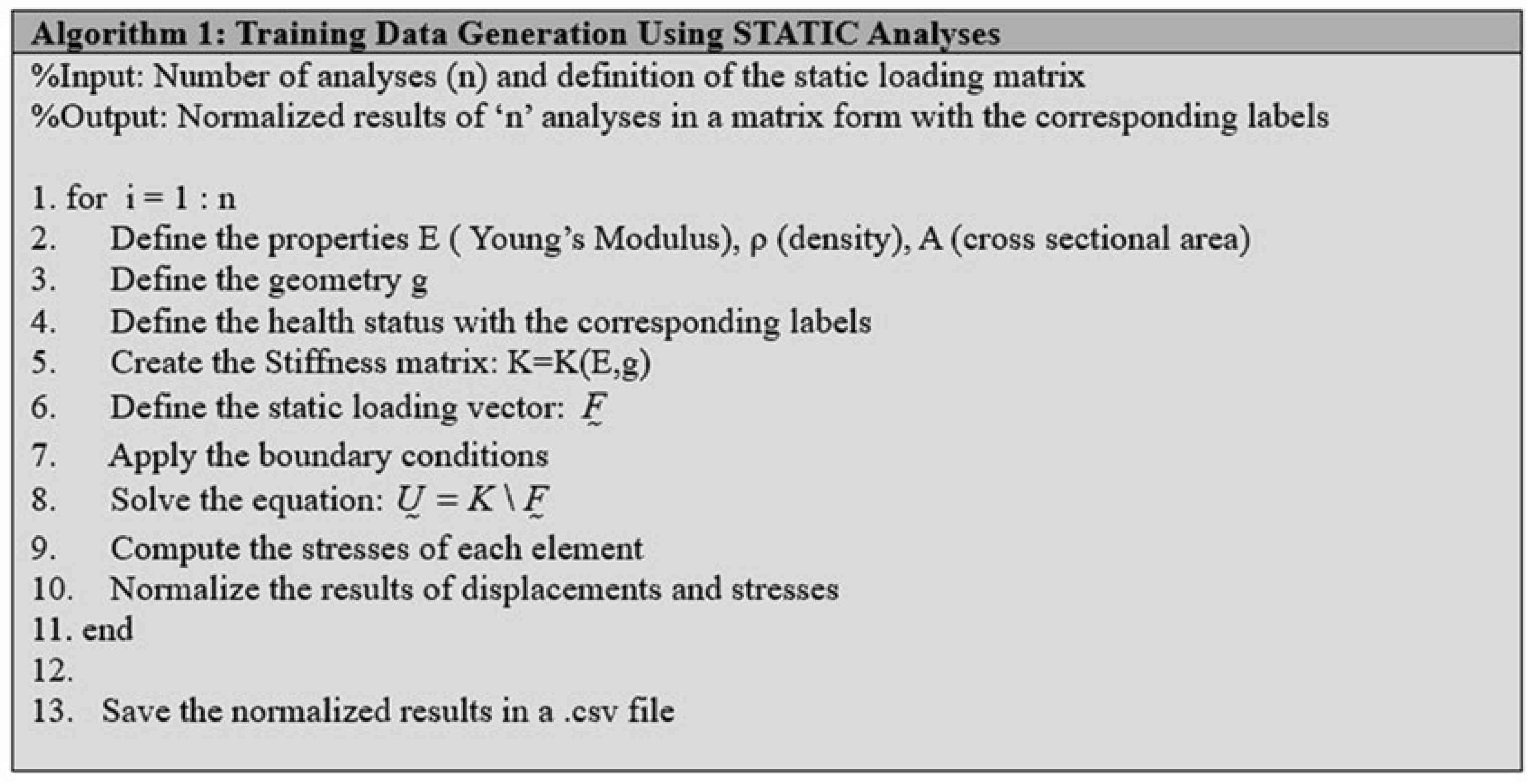
Figure 4.
Regularized results of static analyses with labels, in a matrix form.
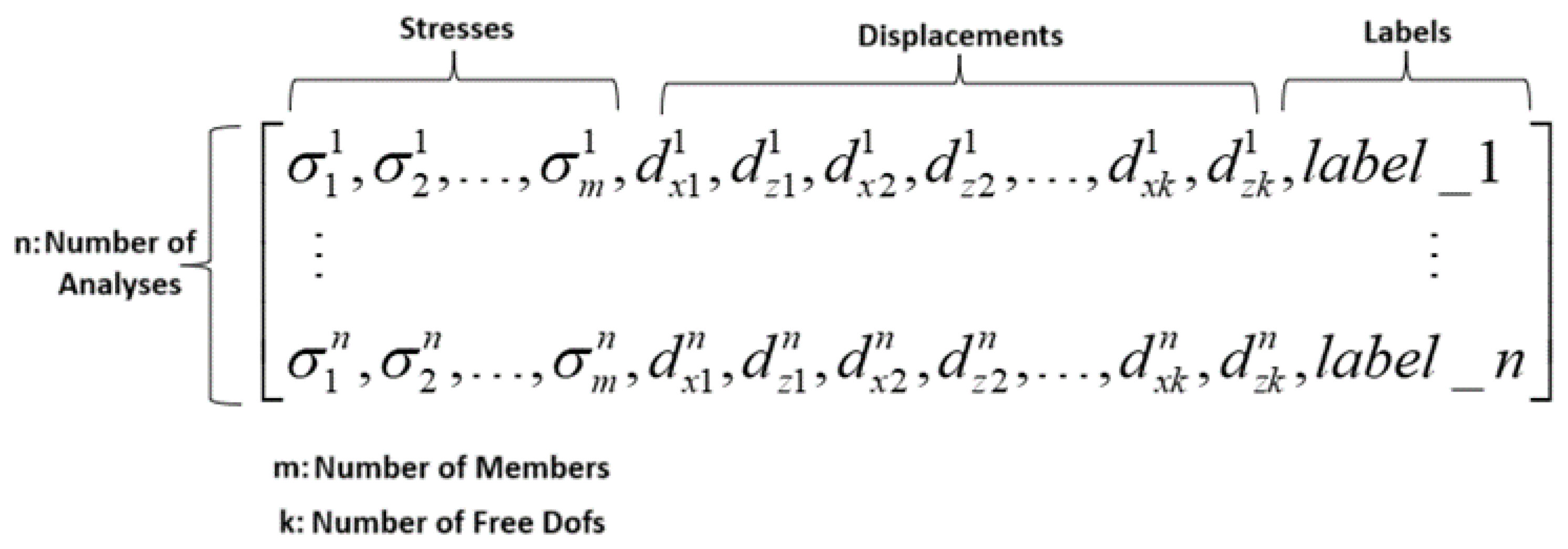
Figure 5.
Algorithm 2.
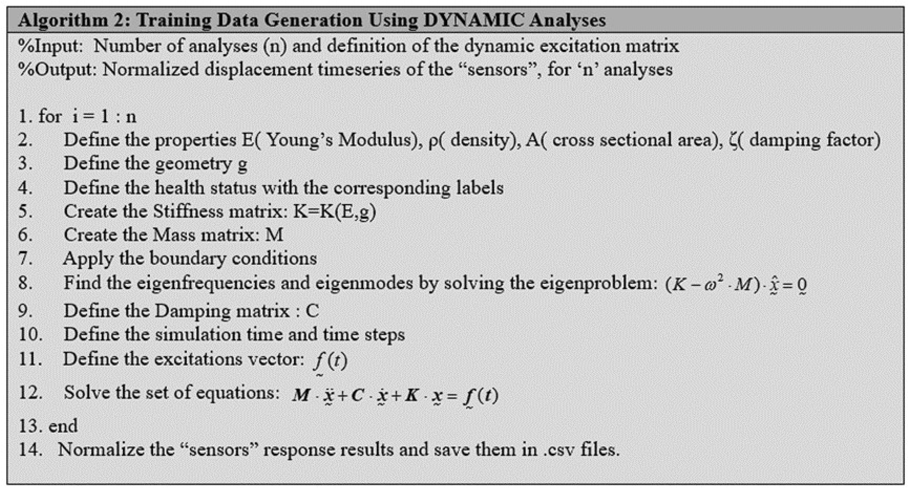
Figure 6.
(a) Schematic representation of dynamic excitations. (b) Random excitation.
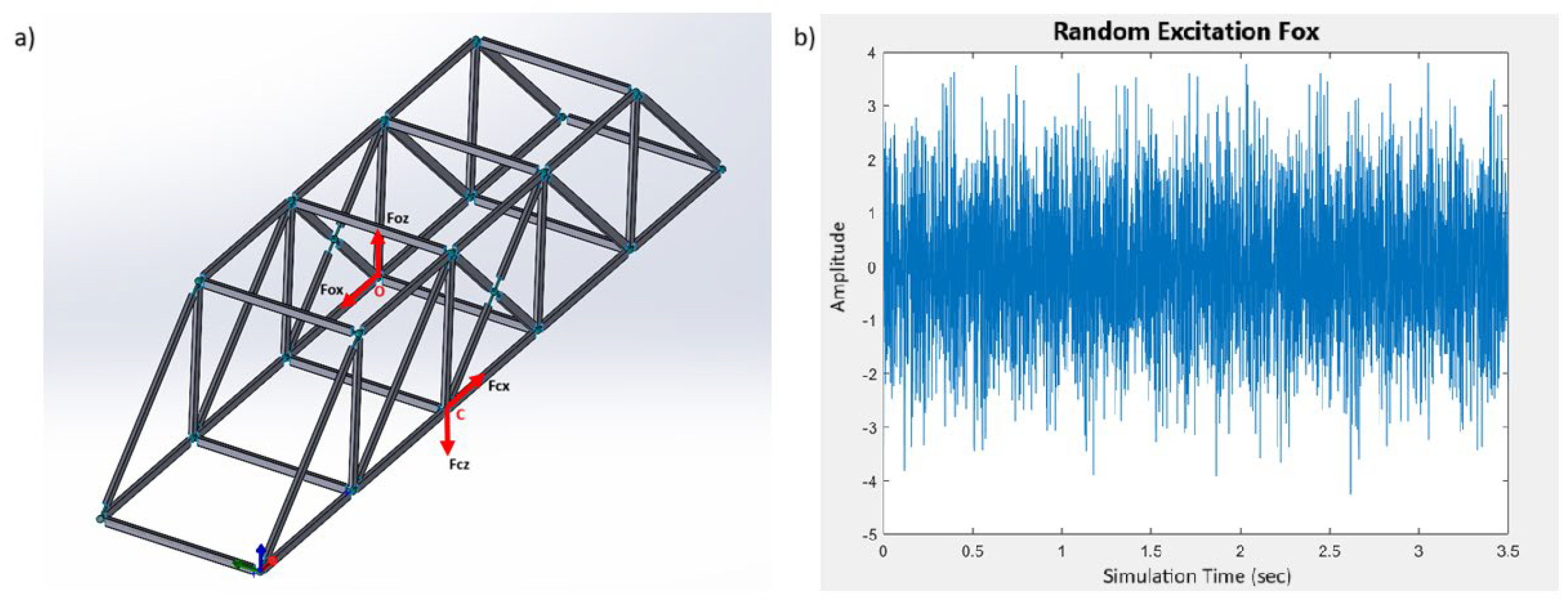
Figure 7.
Schematic representation of channels.
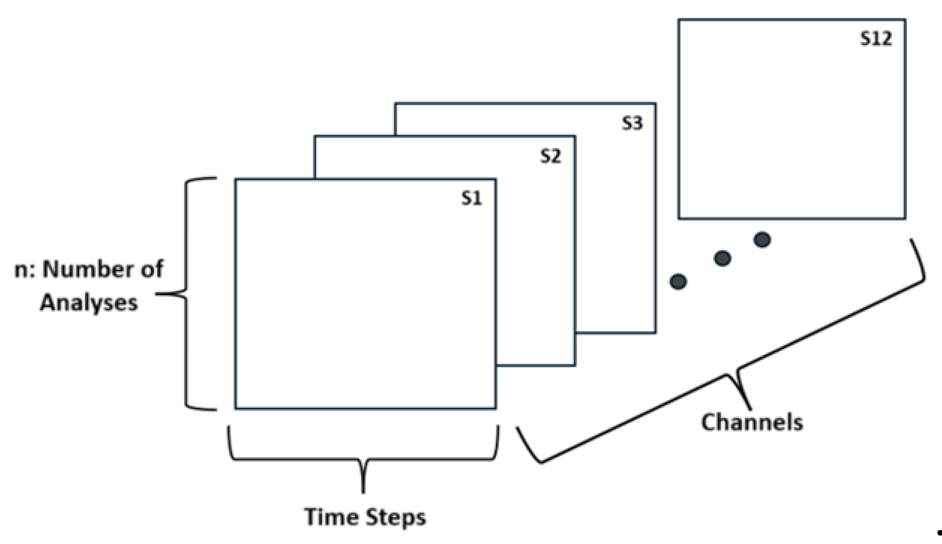
Figure 8.
Meshed bridge geometry with 2D shell elements.
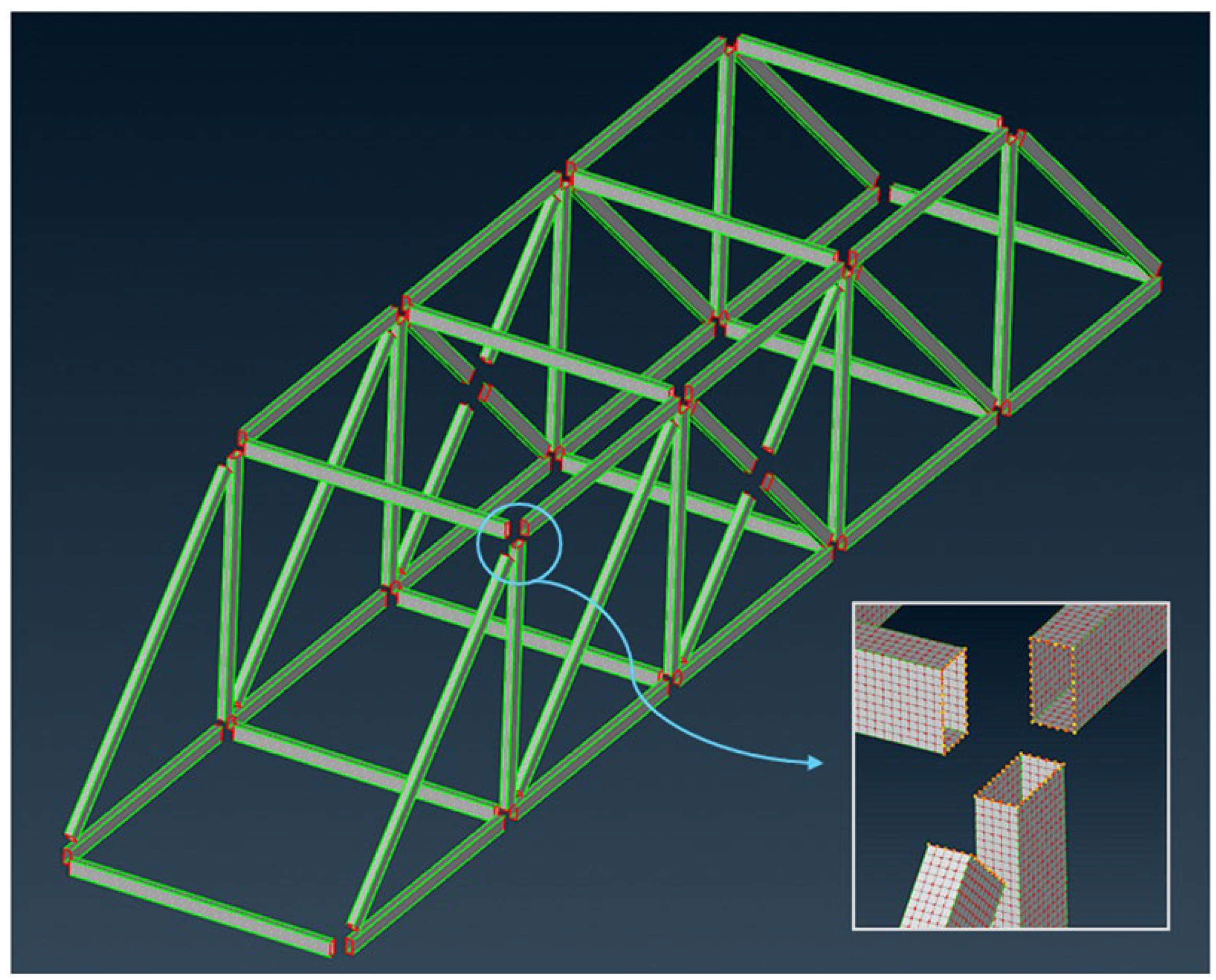
Figure 9.
(a) Modelling of the spherical joint connections with Rigid Body Elements. (b) Demonstration of the boundary conditions.
Figure 9.
(a) Modelling of the spherical joint connections with Rigid Body Elements. (b) Demonstration of the boundary conditions.
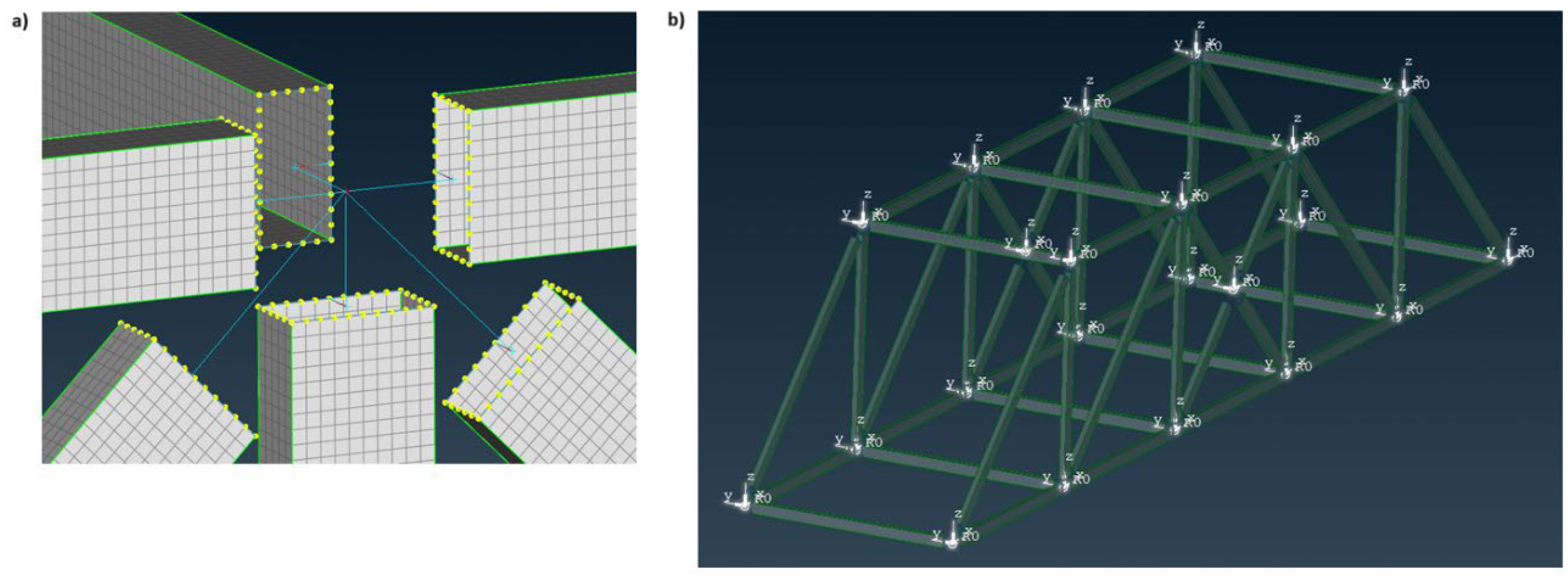
Figure 10.
Architecture of the Neural Networks: (a) Static_minor_damage_DNN. (b) Dynamic_minor_damage_CNN.
Figure 10.
Architecture of the Neural Networks: (a) Static_minor_damage_DNN. (b) Dynamic_minor_damage_CNN.
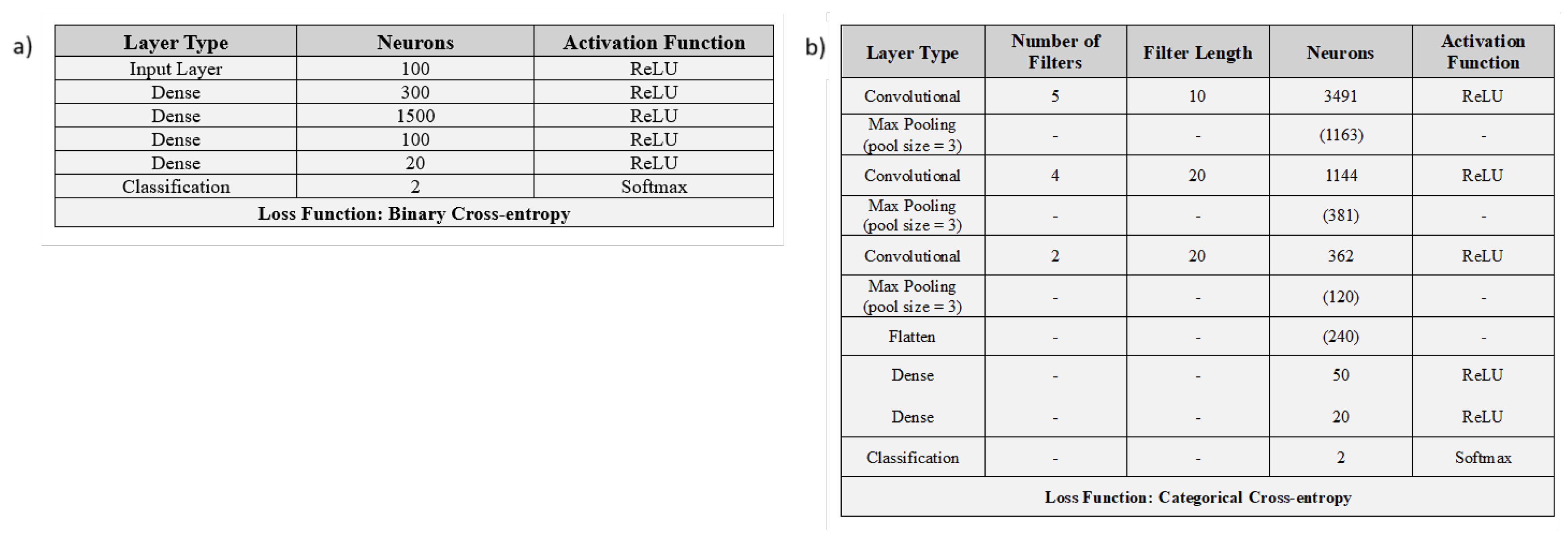
Figure 11.
Training curves of the Neural Networks: (a) Static_minor_damage_DNN. (b) Dynamic_minor_damage_CNN.
Figure 11.
Training curves of the Neural Networks: (a) Static_minor_damage_DNN. (b) Dynamic_minor_damage_CNN.
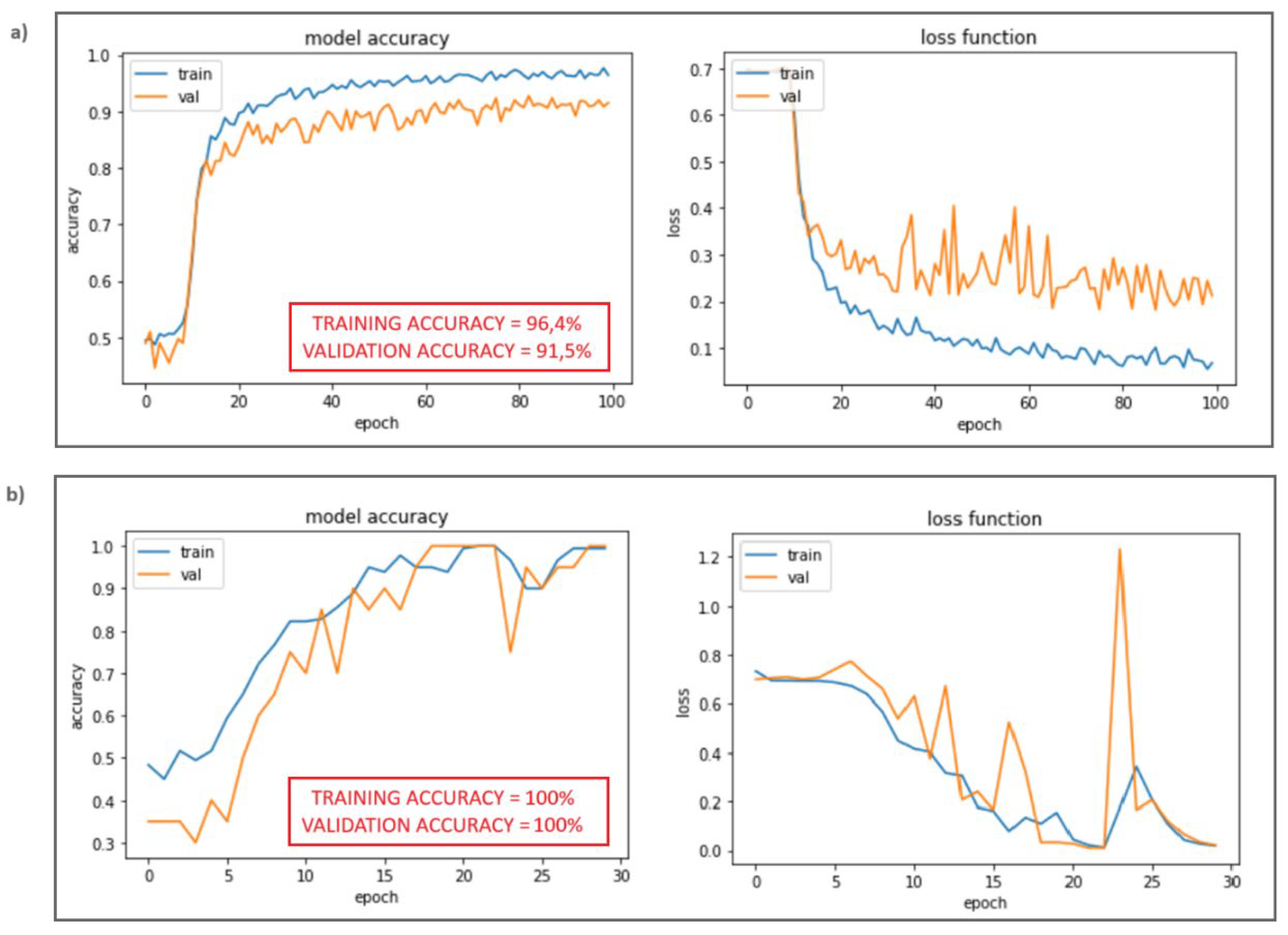
Figure 12.
Architecture of the Neural Networks: (a) Static_extensive_damage_DNN. (b) Dynamic_extensive_damage_CNN.
Figure 12.
Architecture of the Neural Networks: (a) Static_extensive_damage_DNN. (b) Dynamic_extensive_damage_CNN.
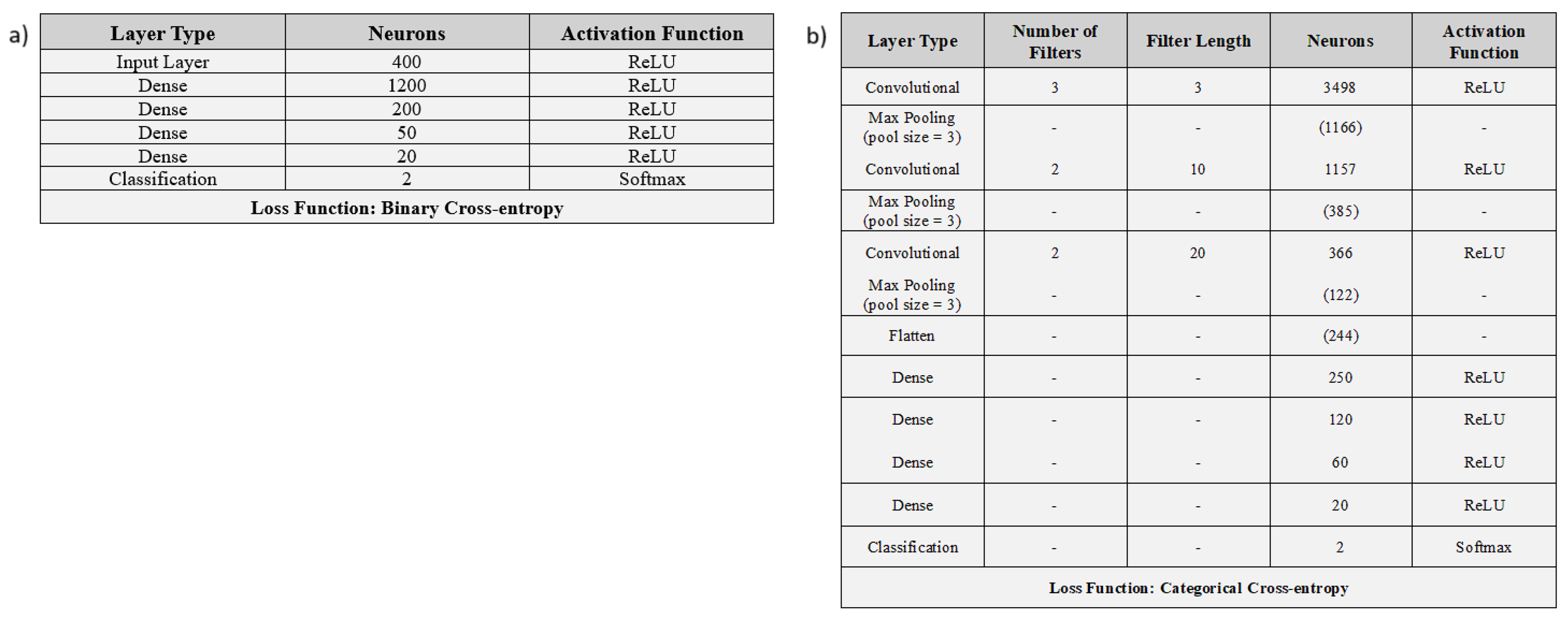
Figure 13.
Training curves of the Neural Networks: (a) Static_extensive_damage_DNN. (b) Dynamic_extensive_damage_CNN.
Figure 13.
Training curves of the Neural Networks: (a) Static_extensive_damage_DNN. (b) Dynamic_extensive_damage_CNN.
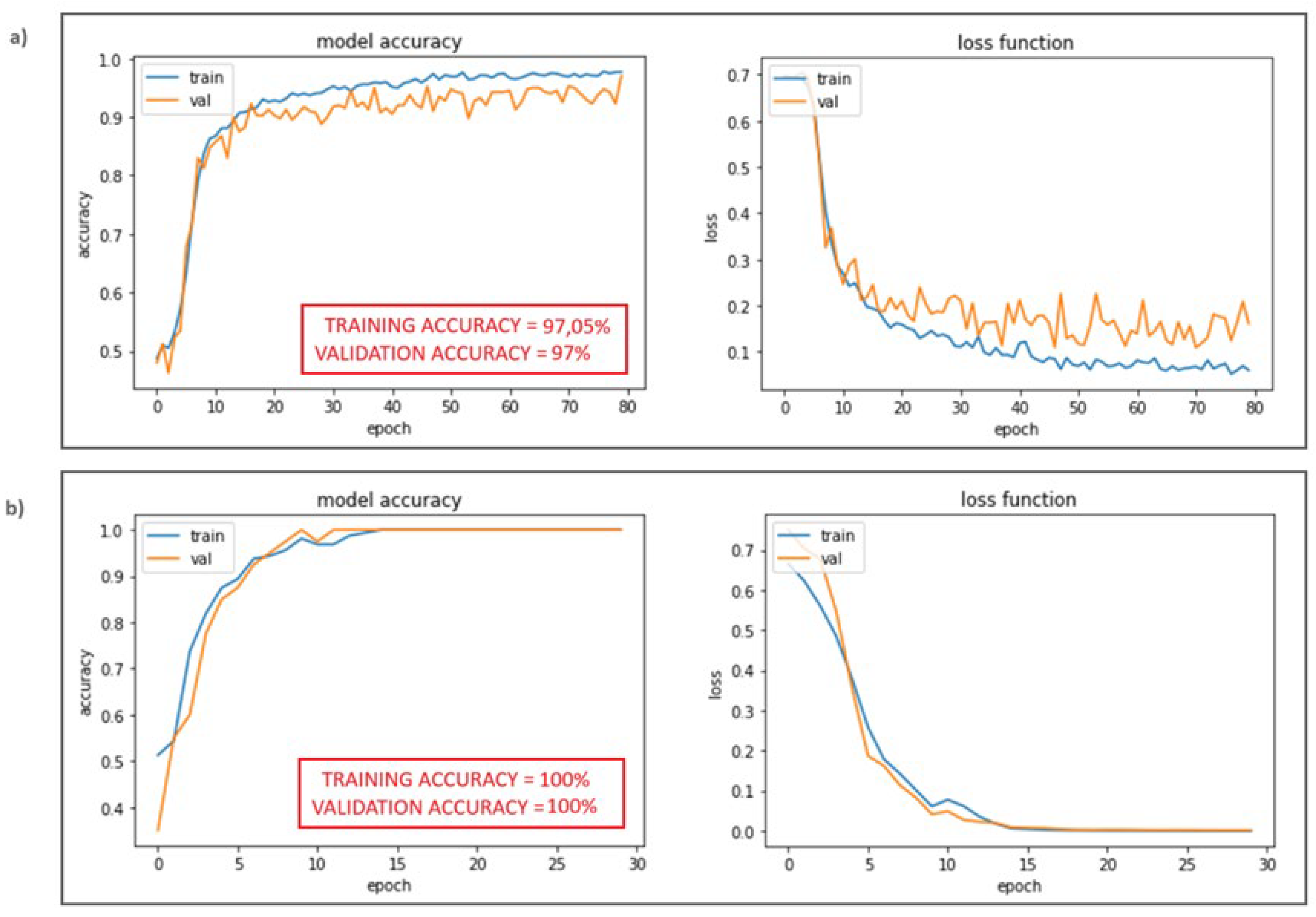
Figure 14.
Schematic representation of the three damage classes.
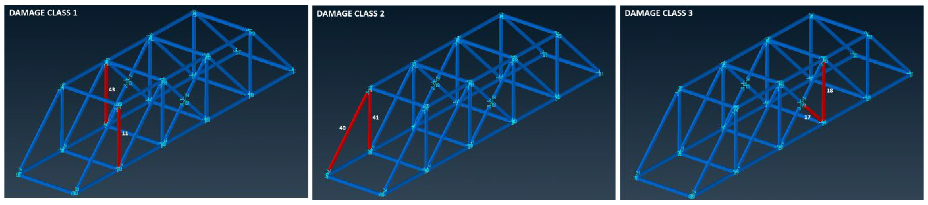
Figure 15.
Architecture of the Neural Networks: (a) Multiclass_static_DNN. (b) Multiclass_dynamic_CNN.
Figure 15.
Architecture of the Neural Networks: (a) Multiclass_static_DNN. (b) Multiclass_dynamic_CNN.
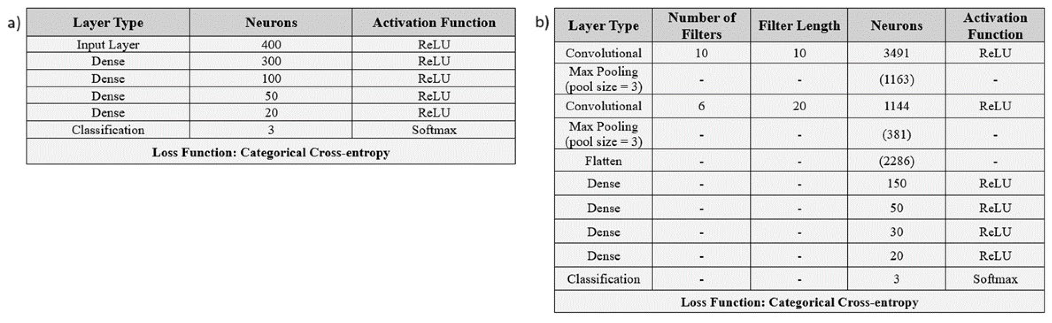
Figure 16.
Training curves of the Neural Networks: (a) Multiclass_static_DNN. (b) Multiclass_dynamic_CNN.
Figure 16.
Training curves of the Neural Networks: (a) Multiclass_static_DNN. (b) Multiclass_dynamic_CNN.
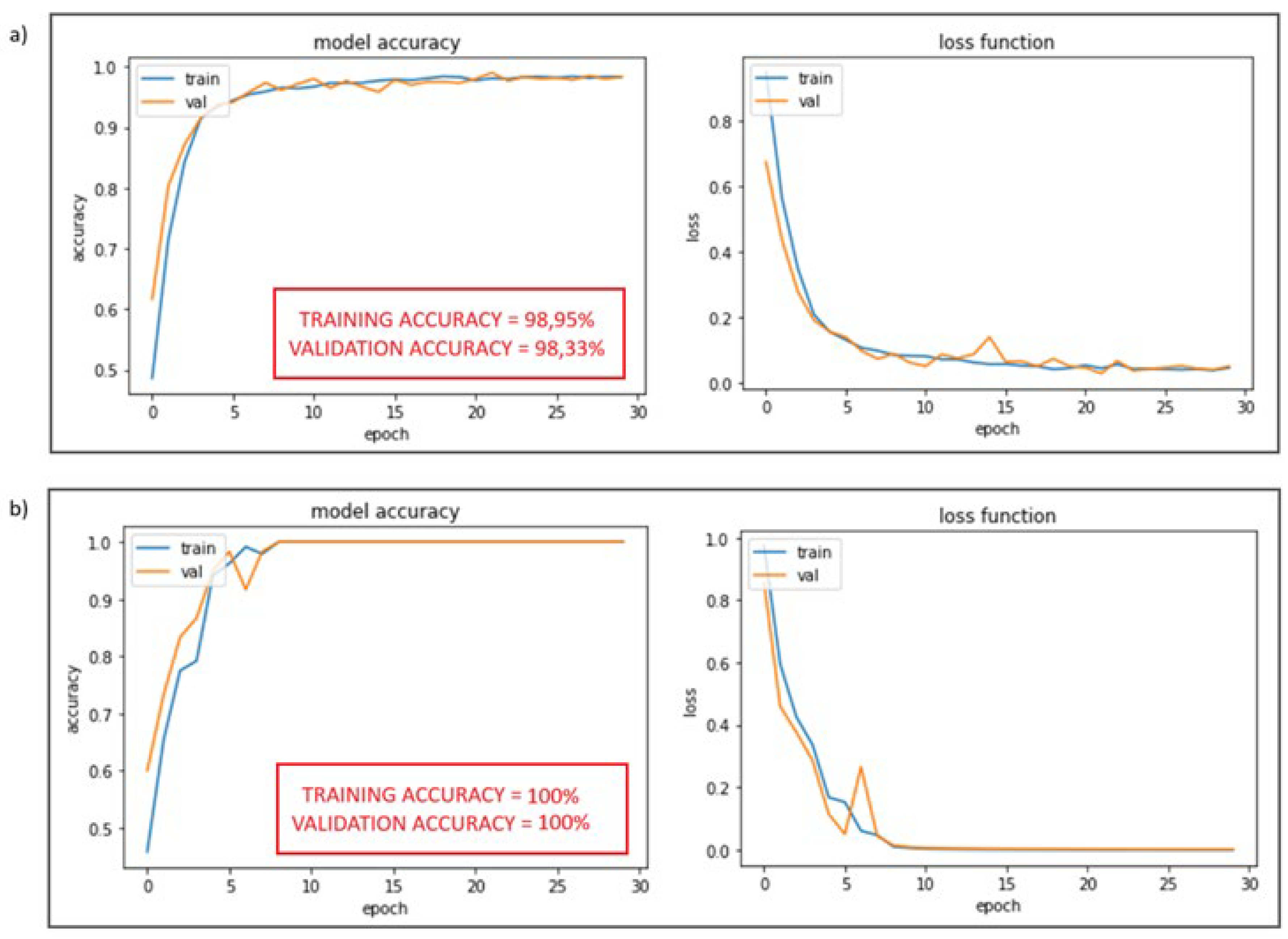
Figure 17.
Confusion matrices for the predicted classes of the trained Neural Networks (Class 1 corresponds to the healthy state of the bridge and Class 2 to the damaged). (a) Static_minor_damage_DNN. (b) Dynamic_minor_damage_CNN. (c) Static_extensive_damage_DNN. (d) Dynamic_extensive_damage_CNN.
Figure 17.
Confusion matrices for the predicted classes of the trained Neural Networks (Class 1 corresponds to the healthy state of the bridge and Class 2 to the damaged). (a) Static_minor_damage_DNN. (b) Dynamic_minor_damage_CNN. (c) Static_extensive_damage_DNN. (d) Dynamic_extensive_damage_CNN.
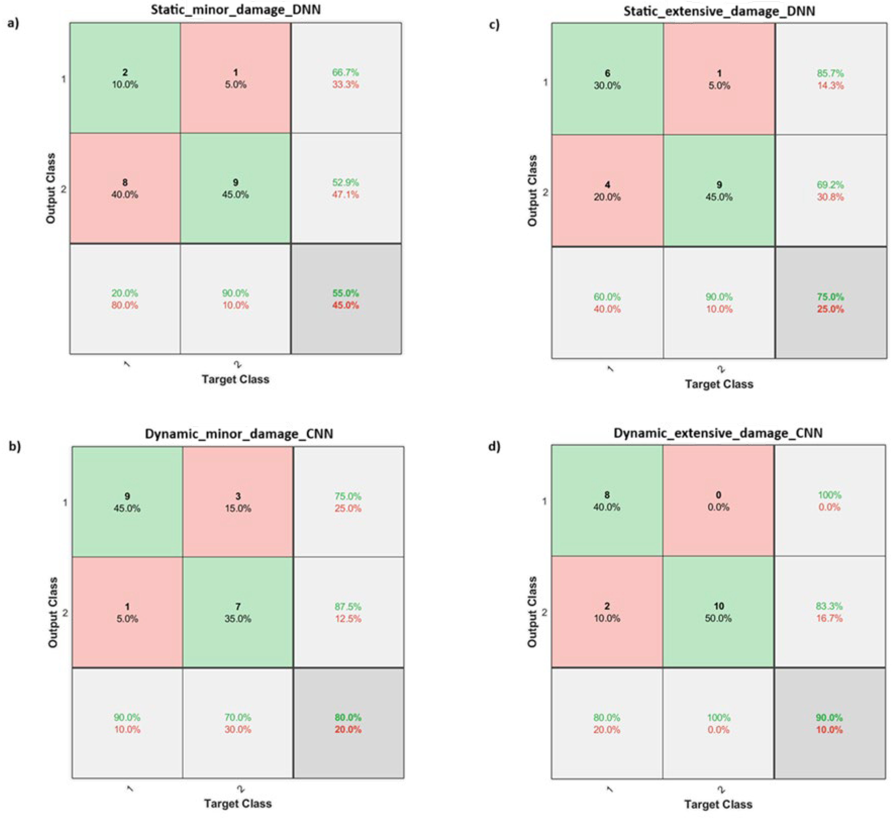
Figure 18.
Confusion matrices for the predicted classes of the trained Neural Networks. (a) Multiclass_static_DNN. (b) Multiclass_dynamic_CNN.
Figure 18.
Confusion matrices for the predicted classes of the trained Neural Networks. (a) Multiclass_static_DNN. (b) Multiclass_dynamic_CNN.
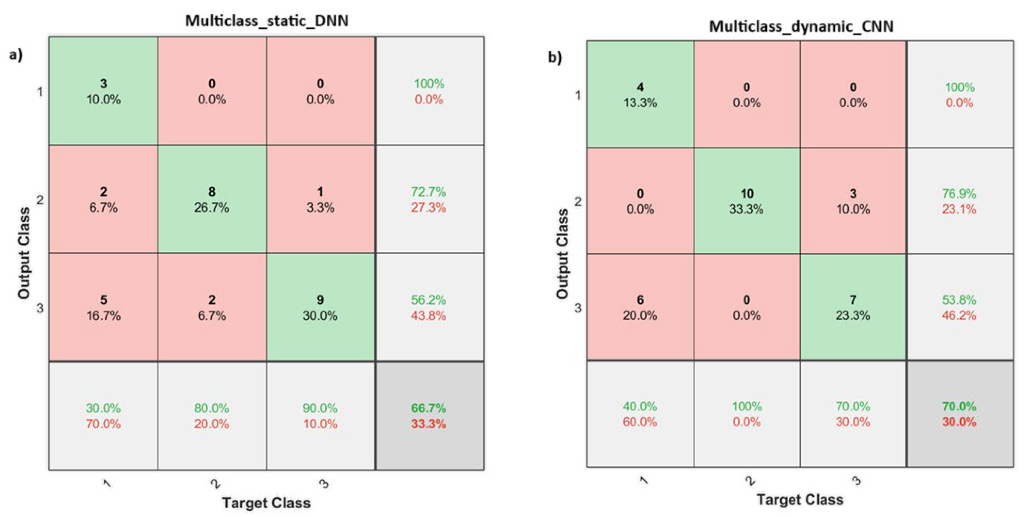
Figure 19.
Bar charts of target and predicted classes. (a) Target classes. (b) Predicted classes from Multiclass_static_DNN. (c) Predicted classes from Multiclass_dynamic_CNN.
Figure 19.
Bar charts of target and predicted classes. (a) Target classes. (b) Predicted classes from Multiclass_static_DNN. (c) Predicted classes from Multiclass_dynamic_CNN.
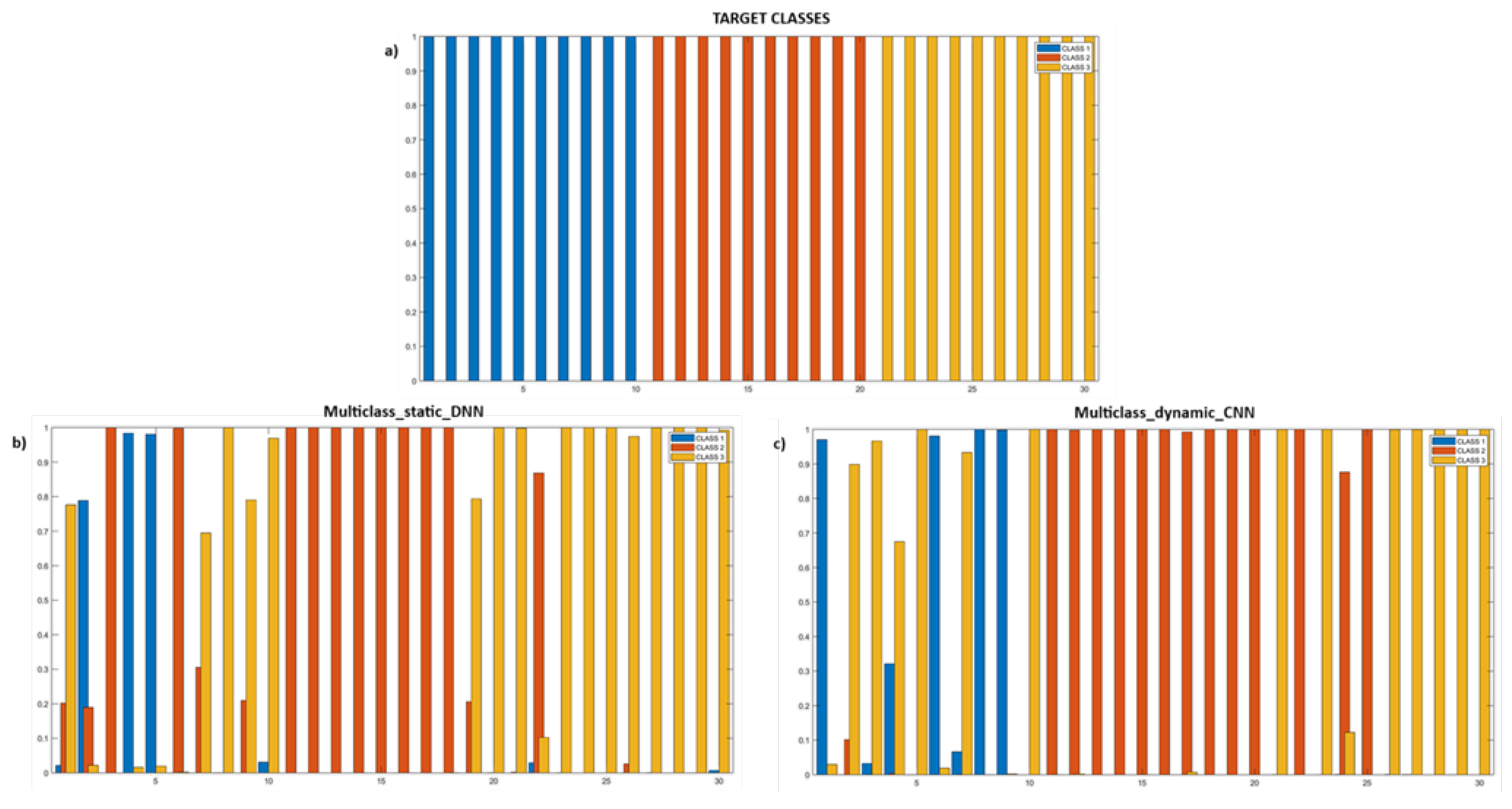

Table 1.
Information about the training of “minor” damage detection Neural Networks.
| ANN Name | Type of FE Analyses | Neural Network Type | Number of Healthy State Analyses | Number of Damaged State Analyses | Training Dataset | Validation Dataset |
| Static_minor_damage_DNN | Static | Deep Neural Network (DNN) | 2000 | 2000 | 3200 (80%) | 800 (20%) |
| Dynamic_minor_damage_CNN | Dynamic | Convolutional Neural Network (CNN) | 100 | 100 | 180 (90%) | 20 (10%) |
Table 2.
Information about the training of “extensive” damage detection Neural Networks.
| ANN Name | Type of FE Analyses | Neural Network Type | Number of Healthy State Analyses | Number of Damaged State Analyses | Training Dataset | Validation Dataset |
| Static_extensive_damage_DNN | Static | Deep Neural Network (DNN) | 2000 | 2000 | 3600 (90%) | 400 (10%) |
| Dynamic_extensive_damage_CNN | Dynamic | Convolutional Neural Network (CNN) | 100 | 100 | 160 (80%) | 40 (20%) |
Table 3.
Information regarding the training of the Multi-Class Neural Networks.
| ANN Name | Type of FE Analyses | Neural Network Type | Number of Class 1 Damage Analyses |
Number of Class 2 Damage Analyses |
Number of Class 3 Damage Analyses |
Training Dataset | Validation Dataset |
| Multiclass_static_DNN | Static | Deep Neural Network (DNN) | 2000 | 2000 | 2000 | 5400 (90%) | 600 (10%) |
| Multiclass_dynamic_CNN | Dynamic | Convolutional Neural Network (CNN) | 100 | 100 | 100 | 240 (80%) | 60 (20%) |
Table 4.
Aggregate prediction results.
| ANN Name | Damage Extent | Prediction Success Rate |
| Static_minor_damage_DNN | Minor | 55% |
| Dynamic_minor_damage_CNN | Minor | 80% |
| Static_extensive_damage_DNN | Extensive | 75% |
| Dynamic_extensive_damage_CNN | Extensive | 90% |
Disclaimer/Publisher’s Note: The statements, opinions and data contained in all publications are solely those of the individual author(s) and contributor(s) and not of MDPI and/or the editor(s). MDPI and/or the editor(s) disclaim responsibility for any injury to people or property resulting from any ideas, methods, instructions or products referred to in the content. |
© 2024 by the authors. Licensee MDPI, Basel, Switzerland. This article is an open access article distributed under the terms and conditions of the Creative Commons Attribution (CC BY) license (http://creativecommons.org/licenses/by/4.0/).
Copyright: This open access article is published under a Creative Commons CC BY 4.0 license, which permit the free download, distribution, and reuse, provided that the author and preprint are cited in any reuse.


