Reframing Forest Harvest Scheduling Models for Ecosystem Services Management

1. Introduction

Linear programming (LP) has been used in forest management planning since the 1960s [1,2,3,4,5,6]. Many variations of these models have been proposed, including, for example, multi-objective models [7,8,9,10,11,12,13,14], spatially-explicit mixed integer programming (MIP) models [15,16,17,18,19,20], and models incorporating uncertainty [21,22,23,24,25,26,27]. While earlier forest planning LP models often considered only one type of management activity – final harvest and regeneration of even-aged management units – since at least Randall [28], analysts have been incorporating a variety of other treatments – such as thinning [28] and coppice harvests [29]. These models originally focused on scheduling timber harvests in even-aged forests to maximize harvest volumes or net present values, but today management objectives include a diverse range of ecosystem services [14,30,31]. Multiple demands on forests for a variety of products and services have led to the development of multifunctional forestry planning models that account for timber and non-timber values and services, such as berry and mushroom picking [32], habitat sustainability, deadwood availability, carbon sequestration, carbon storage [33,34,35,36,37,38], biodiversity conservation indicators [39], and hunting benefits [40].

Johnson and Scheurman [41] identified two fundamental ways to formulate LP forest management planning models, which they named Model I and Model II. Other authors [22,42,43,44] have used a third formulation that has been referred to as Model III [45,46]. While hundreds of papers have been written about LP and MIP forest planning models, most models described in the literature have used Model I [47]. We have found only a few articles that use Model II. Nanang and Hauer [40] use Model II to build a model exploring tradeoffs between timber production and hunting benefits; Diaz-Balteiro et al. [48] present a harvest scheduling model for a community forest; and Grossberg [49] integrates road access to harvest scheduling. While not strictly an LP model, Sessions et al. [50] use simulated annealing to solve a harvest scheduling model with spatial control whose design is based on a Model II MIP. However, at least two forest management software packages used for industrial and agency applications have the option of using Model II. Woodstock Optimization Studio [51], a forest planning application widely used in the forest products industry, and PRISM [52], a U.S. Forest Service application, both allow Model II formulations. We have identified a few articles that use Model III [22,42,43,53,54]. Salo and Tahvonen [44] list Model II in their key words, but their model is better described as Model III.

There usually are multiple ways to formulate any given real-world problem as a mathematical model. When different formulations all produce the same solution, it is useful to assess the advantages and disadvantages of the different formulations, and whether it matters at all which formulation is used. A few papers have compared the relative performance of Model I and Model II. Johnson and Scheurman [41], who introduced Model II, focused on model size and solution time in the context of large LP models, which in 1977 were resource-intensive to formulate and solve given the computing capacity of the time. Their concern with model size led them to focus on the possibility of combining analysis areas that differ only in their initial age class after a final (clearcut) harvest (since the initial age class and stocking are no longer relevant). Barros and Weintraub [55] also focus on the ability to reduce the number of variables in Model II by combining similar management units when they are harvested in the same period. Today, however, model size is seldom a significant concern for non-spatial LP models. However, model size and solution time is (and probably always will be) a concern for spatially explicit models, which generally involve binary variables [16]. However, in spatially explicit models all management units differ in terms of their location, so combining management units following a final harvest negates the ability to model a management unit’s location. McDill et al. [56] and Martin et al. [57] compared Model I and Model II formulations in the context of MIP planning models, focusing primarily on solution time. These papers came to opposite conclusions, with McDill et al. [56] finding that Model II performed better and Martin et al. [57] giving the advantage to Model I. Eriksson [58] compared Model I and Model II in the context of modeling uncertainty and concluded that Model II more easily accommodates a stochastic approach and produces smaller stochastic models due to its tree-graph design, as opposed to the matrix design of Model I. Reed and Errico [22] take advantage of the decision tree structure of Model III for addressing uncertainty related to fire. Based on these few studies, it is difficult to determine whether one formulation is superior for any given application, and one might conclude that perhaps no formulation will consistently outperform another.

Additional criteria could also be considered when comparing different model formulations, including how easy they are to understand and the insight they provide into the structure of the real-world problem being modeled. For example, Model I might have been used more than Model II because it is easier to understand, or because it fits more naturally into the matrix-based structure of a LP model, or simply because more papers use it, so it is the formulation most analysts are familiar with. Especially for large models, storage considerations and model formulation time may also be important. In any case, unless one formulation is uniformly superior to another, having multiple ways to formulate a mathematical model is generally a good thing since one formulation may work better for one situation while another formulation works better for another problem.

The objective of this paper is to revisit Models I, II, and III and consider them from a new perspective. One specific objective of this paper is to encourage forest planning researchers and practitioners to consider using Models II and III more often. One reason these models are not used as much as Model I could be confusion and lack of clarity about exactly how the models are defined. This paper seeks to alleviate such confusion by presenting the three model formulations using a consistent notation that illustrates the key similarities and differences between them and that de-emphasizes the non-essential features of these models that have perhaps received too much attention in the literature and contributed to uncertainty about the models. Our presentation of the models provides insight into their structure, revealing the matrix perspective underlying Model I, and the network – or decision tree – perspectives underlying Models II and III. This difference has also been noted by Garcia [42] in the case of Model III, and Erickson [58] in the case of Model II. Additionally, while both Models II and III have network structures, our exposition shows how Model II focuses on interventions (management actions), while Model III emphasizes the state trajectory of a management unit. This state-focused perspective can be particularly useful when the problem involves objectives or constraints – such as water yields, forest carbon storage, and other ecosystem services – that depend on the state of the forest at any given time, rather than the inputs and outputs associated with interventions.

Another reason to revisit the definition of the Model I, II, and III formulations is to resolve some of the ambiguity that has been propagated in the literature regarding the salient features of these models. Several papers [41,42,55] have emphasized the possibility of combining management units after a final harvest, which can be done with both Models II and III but not with Model I. In fact, Gunn [46], Martin et al. [57], and Nguyen et al. [52] require (as part of the definition of these models) the merging of management units that differ only in their age, stocking or species composition when they are regeneration harvested in the same planning period. While this possibility is a feature of Models II and III, we suggest that it is not a necessary feature, and focusing on this particular difference obscures the most important characteristics of the different models. Furthermore, requiring the merging of management units rules out possible uses of Model II (and to a lesser extent Model III) that do not involve merging management units, yet still have the key features of Model II. If we insist that merging is a required feature of Model II, then what do we call models that otherwise look like Model II formulations (according to the definitions proposed here) but do not allow for the merging of management units following a final harvest?

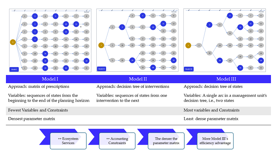
We therefore propose new definitions of Models I, II, and III that do not include (or preclude) merging management units following a final harvest. Our definitions differentiate the models based solely on the sets of periods represented by the model variables. Thus:

In Model I, a variable represents the state of the area assigned to it for an entire sequence of states, interventions, and non-interventions covering the entire planning horizon of the model. In Model II, a variable represents the area assigned to it for one of three sets of periods: 1) the set of periods between two interventions, 2) the set of periods from the initial state to the first intervention, or 3) the set of periods from the final intervention to the end of the planning horizon. In Model III, a variable represents the state of the area assigned to it for one pair of adjacent periods.

Note that we use the term “intervention” in a very general sense here. In this paper, a forest intervention refers to a deliberate management action taken to direct a forest management unit’s expected state trajectory to something different from the trajectory that would have been expected in the absence of the intervention. Thus, interventions could include planting seedlings, an herbicide treatment to control competing vegetation, a thinning, a shelterwood harvest, or an overstory removal, just to name a few possibilities. Most applications of Models II and III have considered final harvest to be the only type of intervention. Garcia [42] discusses the possibility of thinning, but thinning was not included in the actual model described in that paper. Our presentation of these model formulations allows any type of intervention.

It is important to note that when the modeler wishes to combine management units following a final harvest in Model II, they must distinguish between stand-replacing interventions (e.g., final harvests) and non-stand-replacing interventions (e.g., thinnings), as management units can only be merged after stand-replacing interventions. Management units can potentially be combined after a stand-replacing intervention because differences in age, stocking, and even species composition no longer apply. Such differences do not go away with non-stand-replacing disturbances, so merging is not possible following non-stand-replacing disturbances. When management units are merged after stand replacing interventions, it may make sense to define variables in Model II as representing the corresponding area for the set of periods 1) between two stand-replacing interventions, 2) from the initial state to the first stand-replacing intervention, or 3) from the final stand-replacing intervention to the end of the planning horizon. This definition has been used by, among others, Gunn [46], Martin et al. [57], and Nguyen et al. [52]. This variation of Model II would still have the key features of Model II because variables would still represent the state trajectory of a management unit between two disturbances but would not quite fit the definition given above. For those who like clear labels on things, this variation could, perhaps, be called Model IIB, while our definition could be called Model IIA. The distinction between Models IIA and IIB is, of course, moot when final harvests are the only interventions considered, as is often the case. Model IIA can accommodate merging similar areas after regeneration harvests, but one would have to differentiate between stand-replacing interventions and other interventions. We do not consider the merging of management units following a final harvest in the rest of this paper because it would complicate the exposition and possibly perpetuate confusion and ambiguity in the definitions of the three model formulations.

After we review the structure of the Models I, II, and III formulations, the next specific objective of this paper is to assess the advantages and disadvantages of the three models. To do this, we compare the size and performance of each formulation in the context of a case study of strategic planning for the management of a eucalyptus plantation problem in Brazil. The case study illustrates the differences in model size, formulation time, and solution time and when and how different formulations might be preferred. We do not evaluate the performance of the different model formulations in the context of spatially explicit MIP formulations of the forest ecosystem management planning problem. We leave this question for future research.

2. Methods

This section consists of three parts. Section 2.1 to 2.4 specify our formulations of Models I, II, and III. Figure 1, Figure 2, and Figure 3 use decision trees for a single example management unit to illustrate the structure of the three models, emphasizing the differences and similarities in each model’s decision variable definitions, area conservation constraints, and accounting constraints. Particular attention is paid to modeling ecosystem services in harvest scheduling models, as the advantages of the Model III formulation are more apparent when multiple ecosystem services are included in the problem.

Section 2.5 and 2.6 describe a real-world forest ecosystem management problem involving a 12,732-hectare industrial eucalyptus plantation in São Paulo, Brazil, comprised of 350 management units. This forest area is managed primarily to provide pulpwood for a nearby mill, but other ecosystem services, including carbon sequestration and water conservation are also important. This case study will be used to conduct a comparative analysis of the three model formulations in the context of three scenarios, each incorporating an additional ecosystem service.

Section 2.7 details the experimental setup for the case study analysis, including computational resources, solver specifications, and the methodology for running and evaluating the scenarios. It also identifies the performance metrics used to compare the models.

2.1. Example Decision Treee Graph Representation for a Single Management Unit

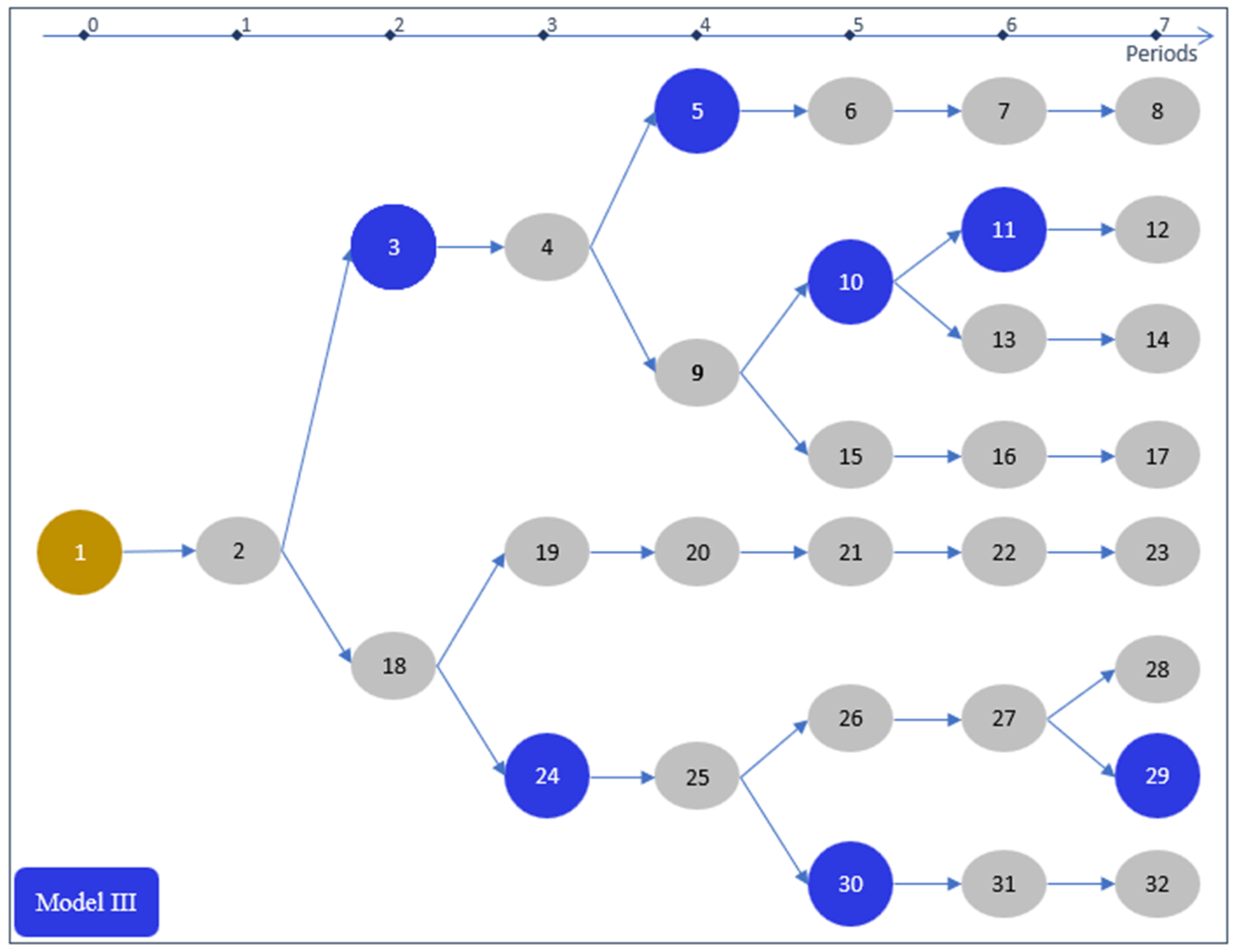
In the following sections, as we describe the three forest management model formulations, it will be useful to visualize how the variables in each model represent the management alternatives for a single example management unit. The alternatives for this example unit are presented as a decision tree in Figure 1. The figure contains three types of nodes: the initial node (brown), non-intervention nodes (gray), and intervention nodes (blue). We do not differentiate between stand-replacing interventions and non-stand-replacing interventions. The specific nature of the interventions is not critical for the example (or for our model definitions), but when the possibility of an intervention exists, the decision tree branches to represent the decision to either implement the intervention (represented by a blue node) or not (represented by a gray node). Thus, for example, in Figure 1 in period 2 there is a decision to either conduct an intervention (node 3) or not (node 18).

Figure 1. Decision tree graph representation of management alternatives for a single example forest management unit. The brown node is the initial node, intervention nodes are blue, and non-intervention nodes are gray.

Figure 1. Decision tree graph representation of management alternatives for a single example forest management unit. The brown node is the initial node, intervention nodes are blue, and non-intervention nodes are gray.

For each model, we first define the sets, variables and parameters needed to formulate the model and then we list the model equations. Alternative equations for a spatially-explicit model are presented following the non-spatially-explicit model formulation. Analogous equations for spatially-explicit models are given the same number, and a prime symbol indicates that an equation is for the spatially-explicit model. As we introduce new models, sets, variables and parameters that have been defined for previous models are not repeated. Following the presentation of the models, Table 1 identifies the sets for each model for the example networks shown in Figure 1, Figure 2, and Figure 3.

2.2. Model I Formulation

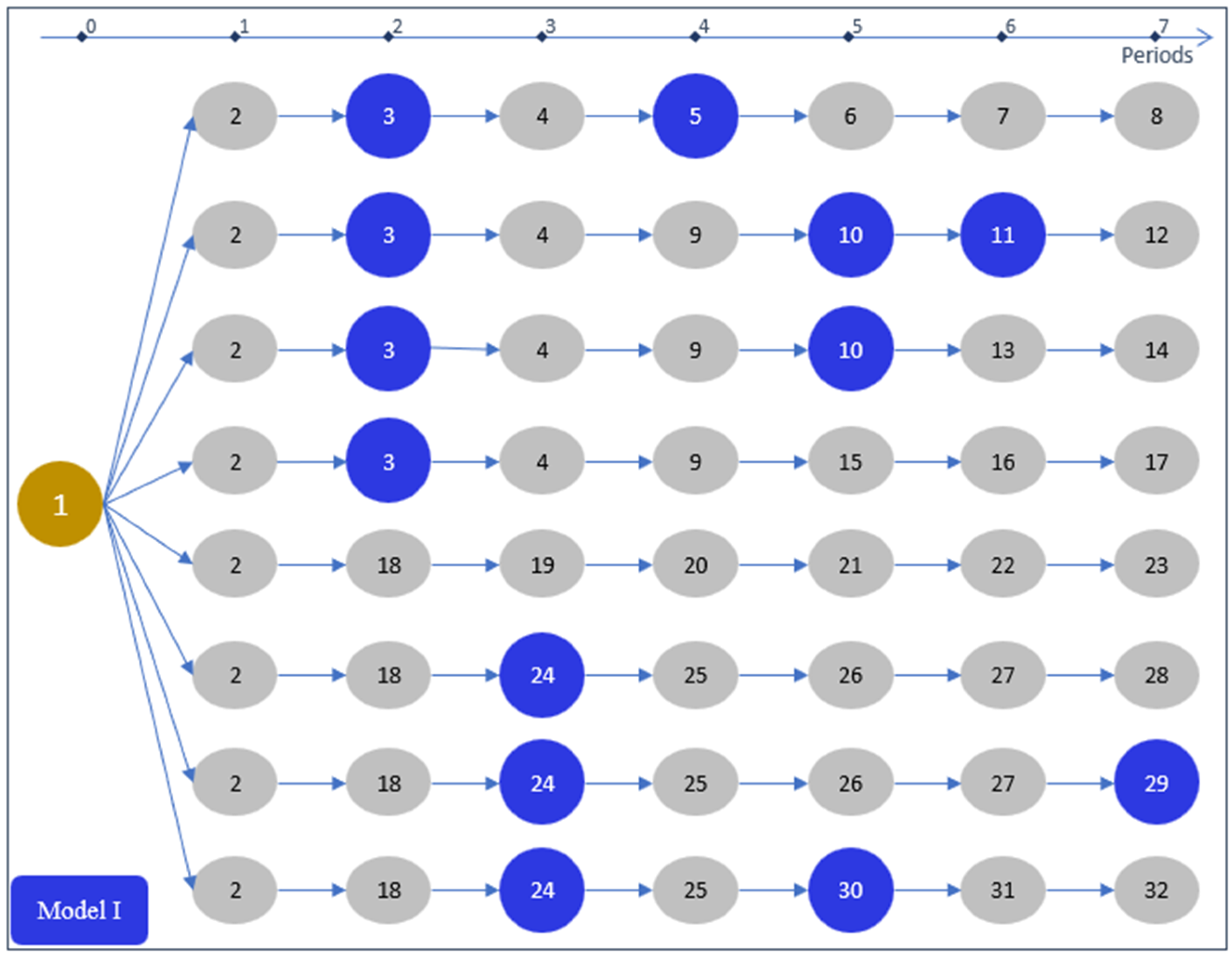
In Model I, each variable represents a complete management alternative for a management unit from the beginning to the end planning horizon. Figure 2 illustrates this by representing the management alternatives from Figure 1 as separate, parallel sequences of nodes corresponding to each complete management prescription. For example, the first prescription is represented by the sequence {1, 2, 3, 4, 5, 6, 7, 8}, and the second prescription is represented by the sequence {1, 2, 3, 4, 9, 10, 11, 12}. In a non-spatially-explicit model, the variable $X_{u1}$ would represent the area of unit u where prescription 1 would be applied. In a spatially-explicit model, the variable $X_{u1}$ would take a value of one or zero, representing, respectively, whether prescription 1 would be applied to unit u or not. The number of Model I variables for a given management unit equals the number of ending nodes in that unit’s decision tree graph.

Figure 2. Model I representation of the management alternatives for the example management unit shown in Figure 1.

Figure 2. Model I representation of the management alternatives for the example management unit shown in Figure 1.

2.2.1. Sets

$\mathrm{e}\in \mathrm{E}$ set of economic quantities, ecosystem services, or landscape conditions (e.g., costs, revenues, timber harvests, timber inventory, carbon stocks or flows, old growth, recently clear-felled area, etc.). For brevity, we will refer to any of these items simply as ecosystem services.

$\mathrm{u}\in \mathrm{U}$ set of management units.

$\mathrm{t}\in \mathsf{{\rm T}}$ set of time periods {min{-t_fu}, …, 0, 1, 2, …, T}; -t_fu represents the time of the most recent (past) intervention for unit u.

$n_u\in N_u$ set of nodes for unit u.

$n_{ut}\in N_{ut}\subseteq N_u$ set of nodes for unit u in a general period t; $N_{ut}$ is a subset of $N_u$.

$n_{uT}\in N_{uT}\subseteq N_u$ the set of nodes for unit u in the specific period T (the last period); these are called “ending nodes.”

$k_u\in K_u$ set of prescriptions for unit u (the term “prescription” is used here to mean a management plan (sequence of interventions and non-interventions) for a single management unit from time 0 to period T, as represented by a connected sequence of nodes from t=0 to T.

Note: there exists a one-to-one mapping from each k_u to each $n_{uT}\in N_{uT}$.

$n_{u{k}_u}\in N_{u{k}_u}$ sequential (ordered), connected set of nodes for unit u that represent prescription k_u.

$n_{u{k}_{u}t}\in N_{u{k}_u}$ node for unit u in prescription k_u for period t (note: there is only one $n_{u{k}_{u}t}$ for period t in prescription $k_u$, but a node may belong to more than one prescription).

2.2.2. Variables

$R_{et}$ equals the quantity of ecosystem service e provided in period t.

Non-spatially-explicit model:

$X_{u{k}_u}$ equals the area of unit u on which prescription k_u will be applied.

Spatially-explicit model:

$X_{u{k}_u}\in \left\{0, 1\right\}$ equals 1 if prescription k_u is applied to unit u, 0 otherwise.

Because there is a one-to-one mapping from each k_u to each $n_{uT}\in N_{uT}$ there is one variable $X_{u{k}_u}$ for each $n_{uT}\in N_{uT}$. For the management unit in Figure 1, there will be eight variables.

2.2.3. Parameters

$r_{u{k}_{u}te}$ the contribution of node $n_{u{k}_{u}t}$ to ecosystem service e in period t. Note that $r_{u{k}_{u}te}$ is stored in the prescription database with the node $n_{u{k}_{u}t}$. In the non-spatially-explicit model, these values are expressed on a per-unit of area basis; in the spatially-explicit model, they are expressed on a per-management-unit basis.

${\lambda }_{et}$ objective function preferential weight for ecosystem service or landscape condition e in period t. For all models it is assumed that $\sum _{t\in T}\sum _{e\in E}{\lambda }_{et}=1$.

$A_u$ the area of unit u.

2.2.4. Formulation

Model I for a non-spatially-explicit forest management problem can now be written as follows:

$$Max {\displaystyle \sum _{\mathrm{t}\in \mathrm{T}}}{\displaystyle \sum _{e\in E}}{\lambda }_{et}{R}_{et}$$

(1)

Subject to

$$\begin{array}{ll}{\displaystyle \sum _{k_u\in K_u}}{X}_{u{k}_u}=A_u& \forall \mathrm{u}\in \mathrm{U}\end{array}$$

(2)

$$\begin{array}{ll}{\displaystyle \sum _{u\in U}}\sum _{k_u\in K_u}{r}_{u{k}_{u}te}{X}_{u{k}_u}-R_{et}=0& \forall \mathrm{e}\in \mathrm{E},\mathrm{t}\in \mathrm{T}\end{array}$$

(3)

$${\displaystyle \sum _{t\in T}}\sum _{e\in E}{\lambda }_{et}=1$$

(4)

$$\begin{array}{ll}{X}_{u{k}_u}\ge 0& \forall \mathrm{u}\in \mathrm{U},k_u\in K_u\end{array}$$

(5)

$$\begin{array}{ll}{R}_{et}\ge 0& \forall \mathrm{e}\in \mathrm{E},\mathrm{t}\in \mathrm{T}\end{array}$$

(6)

Equation (1) defines the objective function as a weighted sum of the economic values, ecosystem services, and landscape conditions produced in each period. Equation Set (2) is the set of area constraints; they state that the sum of the areas from unit u assigned to each prescription must equal the area of unit u. Equation Set (3) is the set of accounting constraints for each ecosystem service and period. Equation (4) states that the sum of the objective function weights equals one. Equation Sets (5) and (6) are non-negativity constraints for the model variables.

For a spatially-explicit model, replace Equation Set (2) with Equation Set (2’) and Equation Set (5) with (5’), as follows:

$$\begin{array}{ll}{\displaystyle \sum _{k_u\in K_u}}{X}_{u{k}_u}=1& \forall \mathrm{u}\in \mathrm{U}\end{array}$$

(2’)

$$\begin{array}{ll}{X}_{u{k}_u}\in \left\{0, 1\right\}& \forall \mathrm{u}\in \mathrm{U},k_u\in K_u\end{array}$$

(5’)

Equation (2’) states that one and only one prescription must be applied to unit u, and Equation (5’) states that the X-variables are binary, i.e., they must equal either zero or one.

Upper or lower bounds on the values or changes in the values of the ecosystem service accounting variables can easily be added to the base model represented by Equations (1) to (6). For example, one could add constraints enforcing minimum or maximum harvest levels, minimum or maximum carbon stored in the forest, minimum levels of carbon accumulation, maximum area of cleared forest within a given zone, minimum area of forest older than a given age, maximum change in the harvest level between periods (flow constraints), etc. The possibilities are too numerous to describe them all here. Adjacency constraints, accessibility constraints, etc. can also be added to the spatially-explicit model. Again, enumerating the possibilities is beyond the scope of this article. It should be noted that a well-constructed model should include constraints on either the ending state of the forest (target forest conditions) and/or include appropriate values for possible ending states in the objective function to ensure accurate valuation of the forest resource and the sustainability of the forest beyond the planning horizon [59].

2.3. Model II Formulation

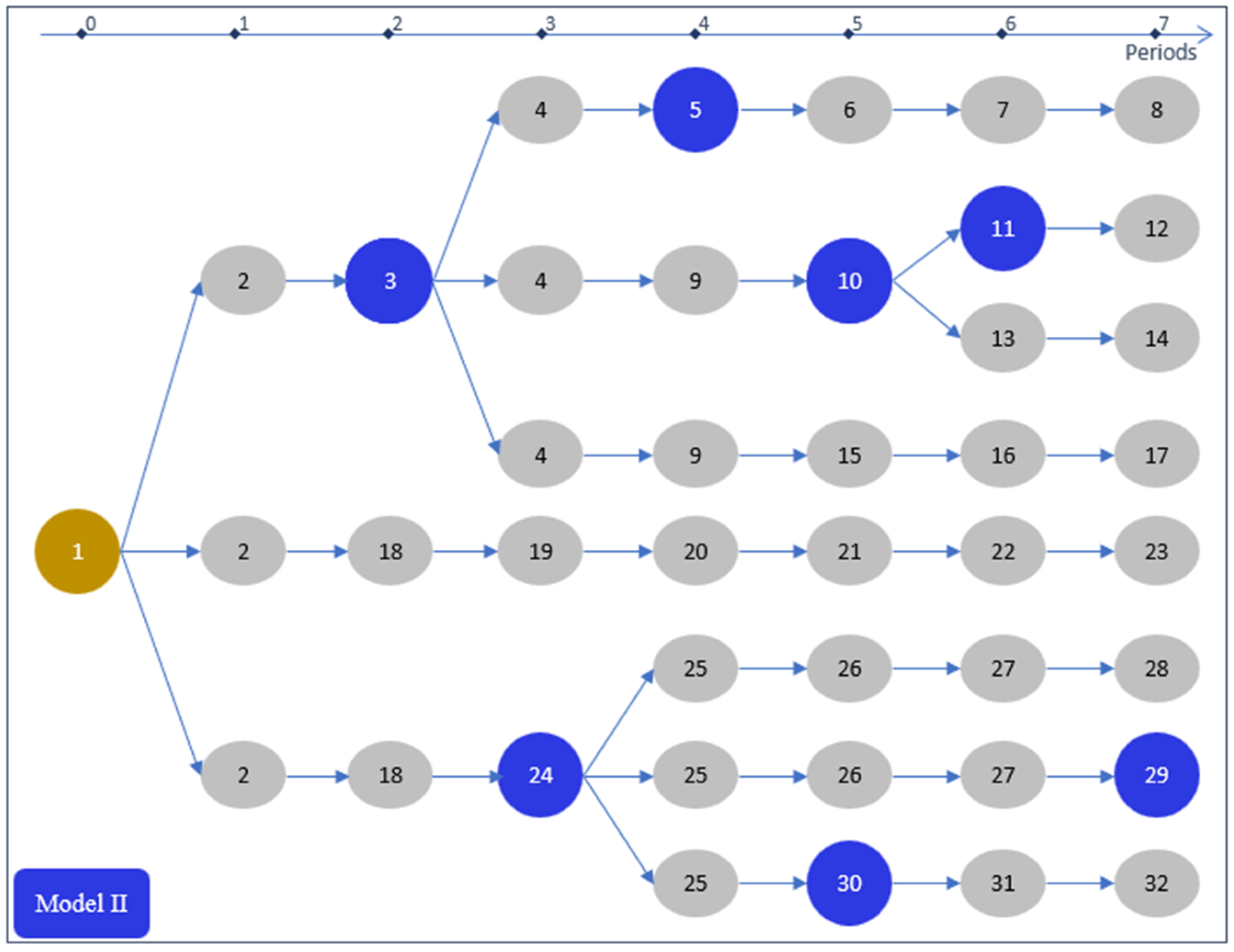
In Model II, each variable represents the state of the area or management unit assigned to it for a period of time (sequence of nodes) that begins either at the beginning of the planning horizon or immediately following a management intervention and that ends either with an intervention or at the end of the planning horizon. Figure 3 illustrates this by representing the alternatives from the example in Figure 1 as they would be represented in Model II. For example, the first variable would represent the sequence {1, 2, 3}, and the second and third variables would represent the sequences {3, 4, 5} and {3, 4, 9, 10}, respectively. In Model II, the number of variables for a given management unit will equal the number of interventions that can be applied to that unit plus the number of non-intervention ending nodes in that unit’s decision tree graph. Equivalently, the number of variables equals the number of intermediate intervention nodes (defined below), plus the number of ending nodes.

2.3.1. New Sets

$n_{u0}$ the initial node for unit u.

$n_u^I\in N_u^I\subseteq N_u$ set of intermediate intervention nodes for unit u; these are nodes that represent an intervention, excluding the initial node (if it is an intervention node) and any intervention nodes that occur in period T; this is why this set is referred to as “intermediate” intervention nodes.

$n_u^{NI}\in N_u^{NI}\subseteq N_u$ set of intermediate non-intervention nodes for unit u; this set includes all non-intervention nodes except the initial node $n_{u0}$ (if it is a non-intervention node) and any non-intervention nodes that occur in period T.

Note that the set $N_u$ can be partitioned into four sets: $N_u=n_{u0}\cup N_u^I\cup N_u^{NI}\cup N_{uT}$.

Figure 3. Model II representation of the management alternatives for the example management unit shown in Figure 1.

Figure 3. Model II representation of the management alternatives for the example management unit shown in Figure 1.

A “prescription” in this model is a sequence of nodes that starts with either the initial node, $n_{u0}$, or an intermediate intervention node, $n_u^I\in N_u^I$, and ends with either an intermediate intervention node, $n_u^I\in N_u^I$, or an ending node, $n_{uT}\in N_{uT}$. Again, let

$k_u\in K_u$ set of prescriptions for unit u.

$n_u^k\in N_u^K=N_u^I\cup N_{uT}$ set of nodes that represent the last node in a prescription.

Note that the set $K_u$ in Model II is different from the set $K_u$ in Model I. Assuming we are not merging similar areas after regeneration harvests, there is a one-to-one mapping from each prescription $k_u\in K_u$ to each $n_u^k\in N_u^K=N_u^I\cup N_{uT}$. Otherwise, there would be a many-to-one relationship between prescriptions in $K_u$ and nodes in $N_u^K$. In our examples, we did not merge similar areas after regeneration harvests.

Define the function $k_u=\mathsf{\Phi }\left(n_u^k\right)$ as returning the prescription $k_u\in K_u$ that ends at node $n_u^k\in N_u^K=N_u^I\cup N_{uT}$.

For each node $n_u^j\in n_{u0}\cup N_u^I$ there is a set of prescriptions that start with node $n_u^j$. Define the set:

$k_u^0\in K_u^0\subseteq K_u$ as the set of prescriptions that that start with node $n_u^0$.

Similarly, define the set:

$k_u^j\in K_u^j\subseteq K_u$ as the set of prescriptions that start with intermediate intervention node $n_u^I\in N_u^I$ (where j is the index to the set $K_u^j$ corresponding to the intermediate intervention node $n_u^I\in N_u^I$; see the definition for $j=\mathsf{\Lambda }\left(n_u^I\right)$ below).

Define the function $j=\mathsf{\Lambda }\left(n_u^I\right)$ that returns the index j for the set $K_u^j\subseteq K_u$ corresponding to the intermediate intervention node $n_u^I$.

$k_u\in K_{ut}$ set of prescriptions for unit u that contain a node in period t.

2.3.2. Variables

The variables in Model II have definitions that appear to be identical to those in Model I. The difference is the prescriptions (sequence of nodes) that they represent.

Non-spatially-explicit model:

$X_{u{k}_u}$ equals the area of unit u on which prescription k_u will be applied.

Spatially-explicit model:

$X_{u{k}_u}\in \left\{0, 1\right\}$ equals 1 if prescription k_u is applied to unit u, 0 otherwise.

2.3.3. Parameters

The parameters are the same as for Model I.

2.3.4. Formulation

Model II can now be written as follows:

$$Max{\displaystyle \sum _{\mathrm{t}\in \mathrm{T}}}{\displaystyle \sum _{e\in E}}{\lambda }_{et}{R}_{et}$$

(1)

Subject to

$$\begin{array}{ll}{\displaystyle \sum _{k_u^0\in K_u^0}}{X}_{u{k}_u^0}=A_u& \forall \mathrm{u}\in \mathrm{U}\end{array}$$

(7)

$$\begin{array}{cc}{X}_{u{k}_u|k_u=\mathsf{\Phi }(n_u^I)}-{\displaystyle \sum _{k_u\in K_u^j|j=\mathsf{\Lambda }(n_u^I)}}{X}_{u{k}_u}=0& \forall \mathrm{u}\in \mathrm{U},n_u^I\in N_u^I\end{array}$$

(8)

$$\begin{array}{cc}{\displaystyle \sum _{u\in U}}{\displaystyle \sum _{k_u\in K_{ut}}}{r}_{u{k}_{u}te}{X}_{u{k}_u}=R_{et}& \forall \mathrm{e}\in \mathrm{E},\mathrm{t}\in \mathrm{T}\end{array}$$

(9)

$${\displaystyle \sum _{t\in T}}{\displaystyle \sum _{e\in E}}{\lambda }_{et}=1$$

(4)

$$\begin{array}{cc}{X}_{u{k}_u}\ge 0& \forall \mathrm{u}\in \mathrm{U},k_u\in K_u\end{array}$$

(5)

$$\begin{array}{cc}{R}_{et}\ge 0& \forall \mathrm{e}\in \mathrm{E},\mathrm{t}\in \mathrm{T}\end{array}$$

(6)

Equation Sets (1), (4), (5), and (6) are the same as for Model I. Equation Set (7) is analogous to Equation Set (2) from Model I, but the summation on the left-hand side is only over the prescriptions that start from the initial node. Equation Set (8) are network flow conservation constraints stating that the total area entering an intermediate intervention node must equal the total area leaving the node. Equation Set (9) is very similar to Equation Set (3); the only thing that has changed is that we only sum over the set of variables that contain a node in period t.

For a spatially-explicit model, replace Equation Set (7) with Equation Set (7’) and Equation Set (5) with (5’), as follows:

$$\begin{array}{cc}{\displaystyle \sum _{k_u^0\in K_u^0}}{X}_{u{k}_u^0}=1& \forall \mathrm{u}\in \mathrm{U}\end{array}$$

(7’)

$$\begin{array}{cc}{X}_{u{k}_u}\in \left\{0,1\right\}& \forall \mathrm{u}\in \mathrm{U},k_u\in K_u\end{array}$$

(5’)

As with Model I, upper or lower bounds on the values or changes in the values of the ecosystem service accounting variables can easily be added to the base model. Adjacency constraints, accessibility constraints, etc. can also be added to the spatially-explicit model. Again, a well-constructed model should include constraints and/or objective function coefficients that ensure accurate valuation of the forest resource and the sustainability of the forest beyond the planning horizon [59].

2.4. Model III Formulation

In Model III, each variable represents a sequence of two nodes that starts with either the initial node, $n_{u0}$, or an intermediate node, $n_u^{Ic}\in N_u^{Ic}=N_u^I\bigcup N_u^{NI}\subseteq N_u$, and ends with either an intermediate node or an ending node, $n_{uT}\in N_{uT}$. Figure 1 shows the Model III representation of the prescriptions for the example management unit. Each variable corresponds to an arc in the network representation in Figure 1. In Model III, the number of variables for a given management unit equals the number of nodes in that unit’s decision tree graph, excluding the initial node. For the example in Figure 1, this would result in 31 prescriptions.

2.4.1. New Sets

$n_u^{Ic}\in N_u^{Ic}=N_u^I\bigcup N_u^{NI}\subseteq N_u$ set of all intermediate nodes (intervention plus non-intervention) for unit u (the “c” superscript indicates that $N_u^{Ic}$ is a combination of $N_u^I$ and $N_u^{NI}$).

Now, the set $N_u$ can be partitioned into three sets: $N_u=n_{u0}\cup N_u^{Ic}\cup N_{uT}$A “prescription” in this model is a sequence of two nodes that starts with either the initial node, $n_{u0}$, or an intermediate node, $n_u^{Ic}\in N_u^{Ic}$, and ends with either an intermediate node, $n_u^{Ic}\in N_u^{Ic}$, or an ending node, $n_{uT}\in N_{uT}$. Now, let

$k_u\in K_u$ set of prescriptions for unit u.

Again, the set $K_u$ in this model is different from the sets $K_u$ in Model I and in Model II. In this model there is a one-to-one mapping from each prescription $k_u\in K_u$ to each $n_u^k\in N_u^K=N_u^{Ic}\cup N_{uT}$. As with Model II, it is possible to merge similar areas after regeneration harvests; if this was done, there would be a many-to-one relationship between prescriptions in $K_u$ and nodes in $N_u^K$.

Define the function $k_u=\mathsf{\Phi }\left(n_u^k\right)$ as returning the prescription $k_u\in K_u$ that ends at node $n_u^k\in N_u^K=N_u^{Ic}\cup N_{uT}$.

For each node $n_u^j\in n_{u0}\cup N_u^{Ic}$ there is a set of prescriptions that start with that node ($n_u^j$). Define the set:

$k_u^0\in K_u^0\subseteq K_u$ as the set of prescriptions that that start with node $n_u^0$.

Similarly, define the set:

$k_u^j\in K_u^j\subseteq K_u$ as the set of prescriptions that start with intermediate node $n_u^{Ic}$ (where j is the index to the set $K_u^j$ corresponding to the node $n_u^{Ic}\in N_u^{Ic}$ ).

Define the function $j=\mathsf{\Lambda }\left(n_u^{Ic}\right)$ that returns the index j to for the set $K_u^j\subseteq K_u$ corresponding to the intermediate node $n_u^{Ic}$.

$k_{ut}\in K_{ut}$ set of prescriptions for unit u that end with a node in period t.

2.4.2. Variables

The variables in the model are again either.

Non-spatially-explicit model:

$X_{u{k}_u}$ equals the area of unit u on which prescription k_u will be applied.

Spatially-explicit model:

$X_{u{k}_u}\in \left\{0, 1\right\}$ equals 1 if prescription k_u is applied to unit u, 0 otherwise.

2.4.3. Parameters

The parameters are the same as for Model I and II.

2.4.4. Formulation

Model III can now be written as follows:

$$Max{\displaystyle \sum _{\mathrm{t}\in \mathrm{T}}}{\displaystyle \sum _{e\in E}}{\lambda }_{et}{R}_{et}$$

(1)

Subject to

$$\begin{array}{cc}{\displaystyle \sum _{k_u^0\in K_u^0}}{X}_{u{k}_u^0}=A_u& \forall \mathrm{u}\in \mathrm{U}\end{array}$$

(7)

$$\begin{array}{cc}{X}_{u{k}_u|k_u=\mathsf{\Phi }(n_u^I)}-{\displaystyle \sum _{k_u\in K_u^j|j=\mathsf{\Lambda }(n_u^I)}}{X}_{u{k}_u}=0& \forall \mathrm{u}\in \mathrm{U},n_u^{Ic}\in N_u^{Ic}\end{array}$$

(10)

$$\begin{array}{cc}{\displaystyle \sum _{u\in U}}{\displaystyle \sum _{k_u\in K_{ut}}}{r}_{u{k}_{u}te}{X}_{u{k}_u}=R_{et}& \forall \mathrm{e}\in \mathrm{E},\mathrm{t}\in \mathrm{T}\end{array}$$

(9)

$${\displaystyle \sum _{t\in T}}{\displaystyle \sum _{e\in E}}{\lambda }_{et}=1$$

(4)

$$\begin{array}{cc}{X}_{u{k}_u}\ge 0& \forall \mathrm{u}\in \mathrm{U},k_u\in K_u\end{array}$$

(5)

$$\begin{array}{cc}{R}_{et}\ge 0& \forall \mathrm{e}\in \mathrm{E},\mathrm{t}\in \mathrm{T}\end{array}$$

(6)

This model appears to be virtually the same as Model II. The only difference in how it is written is in Equation Set (10), which is analogous to Equation Set (8) except that we now have one equation for each intermediate node (not just for intermediate intervention nodes) each management unit. This, and the number of nodes represented by the variables, are the only differences between Models II and III.

For a spatially-explicit model, replace Equation Set (7) with Equation Set (7’) and Equation Set (5) with (5’), as follows:

$$\begin{array}{cc}{\displaystyle \sum _{k_u^0\in K_u^0}}{X}_{u{k}_u^0}=1& \forall \mathrm{u}\in \mathrm{U}\end{array}$$

(7’)

$$\begin{array}{cc}{X}_{u{k}_u}\in \left\{0,1\right\}& \forall \mathrm{u}\in \mathrm{U},k_u\in K_u\end{array}$$

(5’)

To help readers follow the above descriptions of Models I, II, and III, Table 1 lists the key sets from the three models and identifies the nodes belonging to each set from the example prescriptions in Figure 1.

2.5. Case Study Forest Ecosystem Management (FEM) Problem Description

To compare various attributes of Models I, II, and III, we created a case study management problem for an area of fast-growing eucalyptus plantations managed by an integrated forest products company in São Paulo, Brazil. The plantations in the case study are managed using a short-rotation coppice and renewal regime with the primary objective of pulpwood production. The total area to be managed is comprised of 350 management units totaling over 12,732 hectares. Silvicultural interventions include clear-cuts followed by renewal (CCR) or sprouting (coppice) from stumps (CCS) at ages 6, 7, and 8 years, extending to 11 years in the first three periods for older management units. This regime aligns with regional practices, allowing only one CCS before a mandatory CCR.

Inventory, harvest volume, and current annual increment (CAI) for three site index classes (23, 26, 29 m) were determined using yield curves provided by the company. The mean annual increments at age seven (MAI₇) are 26.96, 31.40, and 36.73 m³/haꞏyear in the first rotation and 22.92, 26.69, and 31.22 m³/haꞏyear in the second rotation for the three site classes, respectively.

Genetic material, mostly Eucalyptus grandis, Eucalyptus urophylla, or their hybrids, were grouped by basic wood density (BWD) properties into four categories that influence the carbon sequestration calculations. The high, medium, low, and very low-density groups range from 0.463 to 0.531, 0.446 to 0.503, 0.403 to 0.488, and 0.355 to 0.481 t/m³, respectively, depending on the stand age.

The company provided the initial state of each management unit, including location (region, sub-region, and site index), genetic material, area, and last intervention time and type. The planning horizon was 21 years, divided into one-year planning periods – enough time for three typical rotations.

Carbon sequestration calculations were based on Sanqueta et al. [60], utilizing the Biomass Expansion Factor (BEF), Root Shoot Ratio I (R), and Biomass Carbon Fraction Factor (BCF). We used eucalyptus data collected in a similar region from Ribeiro et al. [61], giving us the factors BEF = 1.2220, R = 0.1689, and BCF = 0.4323 (all three factors are ratios with no units).

Additionally, the company reported natural forest coverage per subregion, where they must maintain at least 20% of the area in natural forests to meet Brazilian regulations. Sub-regions were used as a proxy for micro-watersheds to calculate water-related ecosystem services (ESw). A threshold of 20% of natural forest coverage must be maintained in a micro-watershed with eucalyptus plantations, below which ESw supply tends to become unsustainable; and a level of 45% is desirable for achieving the highest ESw gains [62]. These data and policies, based on concepts from Lima and Zakia [63], are used in our third scenario that considers ESw, as described in more detail below.

Production costs (Table 2; BRL = Brazilian reais, also represented by R$) were provided for two regions. A conservative interest rate of 6% was chosen to avoid biasing the model towards early harvesting [64,65]. A pulpwood price of R$ 100.00/m³ was used based on typical prices in the region. We used a social value of carbon as a proxy for the carbon value, which is R$ 120/t of CO₂ in Brazil [66,67].

We calculated terminal values (TV) following the methodology outlined by Kanieski da Silva et. al. [59], accounting for regional cost differences and production variations specific to each region and site index. First, we determined the management regime that maximizes the Land Expectation Value (LEV) for each region and site index (Table 3). Then a Forest Value [68] was calculated by age, region, and site assuming this management regime would be followed in perpetuity after the planning horizon. These values were applied based on the projected state of the management unit at the end of the planning horizon and discounted to the present like all other values using a 6% discount rate.

All values, tables, and assumptions from this section, including the initial state by management unit, genetic material BWD, required forest cover per sub-region, production tables, costs, LEV, TV for each potential ending condition, formulas, and a Visual Basic macro for TV calculations, are provided in the supplementary material. These data are compiled in an Excel® spreadsheet titled “Assumptions.xlsm,” along with detailed carbon calculation methodologies.

Lastly, we utilized iGen by Romero® [69] to generate all possible management alternatives for this FEM problem. iGen produced a tree graph similar to Figure 1 for each management unit, resulting in a total of 426,191 nodes for all management units. It calculated a suite of parameters for each node for use in formulating the linear programming models, including age, inventory, harvest volume, discounted revenue and costs, carbon sequestration, forest cover, and an age control indicator for the ESw scenario. Additional variables maintained during alternative generation, such as region, sub-region, management unit, area, site index, period, intervention type, rotation, and genetic material, along with the rules and equations of motion, are detailed in an Excel® spreadsheet “Alternatives.xlsx,” available in the supplementary material.

The node data were read to build non-spatial Models I, II, and III according to the formulations described in the previous sections. While Section 2.2, 2.3, and 2.4 describe both non-spatial and spatially-explicit versions of their respective models, including spatially-explicit versions of the case study models was beyond the scope of this analysis. In addition to a base case that considers only the profitability of timber production, two additional scenarios were considered with each scenario adding additional management objectives (ecosystem services). These scenarios are detailed in the following section. With three scenario and three formulations, we created and solved a total of nine LP models.

2.6. Scenarios Description

This study hypothesizes that the relative performance of Models I, II and III varies as the number of Ecosystem Services (ES) included in the model increases. Specifically, we expect Model III to perform better than Models I and II as more ESs are included. To examine this, we have structured three scenarios with escalating complexity. Scenario 1 is a standard timber production harvest scheduling model that serves as the base case. Scenario 2 adds carbon sequestration to Scenario 1 as an additional ES management objective. Finally, Scenario 3 adds an additional water-related Ecosystem Services (ESw), resulting in the most complex scenario for our analysis.

2.6.1. Scenario 1 – Harvest Scheduling

Scenario 1 focuses on timber production, including revenue from timber revenue, the costs of silvicultural activities, and the terminal value. The objective function was to maximize the Net Present Value (NPV) of these three factors. The model includes flow constraints limiting the variation in timber production to ±5% between periods starting from period four. An adjustment period during the first three periods allows more flexibility, which is needed due to an existing backlog of older management units.

The parameters necessary for this scenario – VolCut (volume of timber cut), DscTmbCst (discounted timber costs), DscTmbRev (discounted timber revenue plus discounted terminal value) – were calculated using iGen, as detailed in the previous section. During the model-building phase, accounting constraints and variables were defined by period for VolCut, DscTmbCst, and DscTmbRev. The VolCut accounting variables were used to build the flow constraints, while DscTmbCst and DscTmbRev were utilized to build the NPV objective function.

2.6.2. Scenario 2 – Carbon Analysis

In Scenario 2, we expanded the model to include carbon sequestration and its associated value. A new parameter, CRemoved (carbon removed from the atmosphere), was introduced and calculated by iGen. CRemoved quantifies the CO₂ in tons per hectare removed from the atmosphere and fixed in the trees’ biomass (above and below ground) during the current period. In this scenario, the revenue parameters, which previously included only timber revenues and terminal values, were adjusted to include the value of carbon sequestration, obtained by multiplying the amount of carbon removed by the social cost of carbon and then discounting. Similarly, the cost parameters were adjusted to account for carbon emissions resulting from harvesting, calculated by multiplying the carbon content in the harvested volume by the social cost of carbon. We also introduced a new set of non-declining carbon sequestration constraints stipulating that CRemoved must not decrease over time. The objective function remains the Net Present Value (NPV), which now combines the carbon value with the timber revenue, terminal values and cost components.

The harvest flow constraints from Scenario 1 were also included in this model. Thus, the parameters in this scenario include VolCut (volume of timber cut), DscCosts (discounted costs), DscRevenue (discounted revenue), and CRemoved (carbon removed), used again while building the accounting constraints to compute the corresponding accounting variables, which in turn inform the flow and non-declining carbon constraints, as well as the NPV maximization objective function.

2.6.3. Scenario 3 – Timber, Carbon, and Water

In Scenario 3, we introduced binary parameters, PltCover, to represent the water protection ecosystem service (ESw). PltCover equals 1 when a plantation’s age is two years or older, and 0 otherwise. PltCover is used in a set of accounting constraints to calculate the plantation coverage (the area of soil covered by forest plantations that are at least two years old) within each micro-watershed for each period. Bounds were placed on the resulting accounting variables to set a minimum level of two-year-old or older plantation coverage per period in each micro-watershed.

This scenario also incorporated an age control variable to calculate the weighted age by area, computed as the age multiplied by the area represented by each variable divided by the total area (12,732.41 ha) for every period. Accounting constraints were added to populate accounting variables to track the average age of the forest per period. Non-declining age (NDAge) constraints were added to ensure that this weighted age could not decrease over time because older fast-growing plantation covers are closer to natural forest cover for improving water-related ecosystem services [63].

This scenario retains the constraints from Scenarios 1 and 2, including flow constraints and non-declining carbon. The objective function is the same as Scenario 2, maximizing the Net Present Value (NPV), including the social value of carbon.

2.7. Experimental Setup

iGen by Romero® [69] as used to generate management alternatives and calculate the associated parameters. Data were stored in a remote SQL Server 2022 database [70]. The model-building process for Models I, II, and III was executed through custom software developed in Python 3.9 [71], utilizing SQLAlchemy 2.0.16 [72] and Pandas 2.2.0 [73] packages for database connectivity.

Pyomo 6.7.1 [74], a Python based algebraic modeling language (AML), was used to construct the optimization models. Pyomo interfaces with the Gurobi Optimizer version 10.0.3 win64 [75] to solve the models. Results and comprehensive control logs detailing each step of the process are saved back to the original SQL Server database containing the model formulation data. These logs are instrumental for the analysis presented in the results.

All tests were conducted on a local computer equipped with an 11th Gen Intel® Core™ i7-1165G7 CPU @ 2.80GHz, 64GB RAM, featuring four physical cores, eight logical processors, and support for up to eight threads. To ensure the accuracy and integrity of the tests, we turned off all non-essential software to prevent interference with CPU and memory usage. The test suite, encompassing nine runs (three scenarios across three models), was executed in a controlled environment to eliminate the influence of external applications on computing resources.

Case study results compare model sizes (numbers of variables, constraints, and non-zero coefficients), and formulation and solution times. We compare details such as the time to formulate each model component and model size before and after pre-solving.

3. Results

As one would expect, Model I formulations had the fewest decision variables per management unit (240), Model II formulations had an intermediate number (421), and Model III had the most (1,218) (Table 4). Model I also has an order of magnitude fewer conservation of area constraints compared to Model II and two orders of magnitude fewer than Model III (Table 4). Conservation of area rows include Equation Set (2) for Model I, Equation Sets (7) and (8) for Model II, and Equation Sets (7) and (10) for Model III. In Model I, the number of conservation area rows equals the number of management units. If we consider only model size, as measured by numbers of variables and constraints, Model I is clearly superior. But there are other, perhaps more important, metrics that should be considered.

We tracked the time for each process phase, from data retrieval from the iGen database to saving the results. Table 5 summarizes the durations of each modeling phase for each scenario and model. Objective function values are also shown in the table to confirm that the three models are indeed solving the same forest management problem.

Data retrieval time is influenced by database organization, database dialect, and internet connectivity rather than model characteristics. Time for this phase varies minimally across models and scenarios, attributed to the consistent number of records processed, predetermined by the number of alternatives generated by iGen in an earlier phase. Minor time differences are due to the time to prepare different parameter sets for the building phase.

In all cases, Model III requires the least model building time, compared with Models I and II, with greater differences in more complex scenarios. For instance, Model III requires only 38% of building time required for Model I in Scenario 1, compared with only 27% of the Model I building time in Scenario 3. This is also the case, but to a lesser degree, when Model III is compared to Model II.

Model II consistently has the lowest solver time, while Model I requires the largest solver time for Scenarios 2 and 3. However, the difference between Models II and III narrows in more complex scenarios. For example, for Scenario 1 it takes almost twice as long to solve Model III compared with Model II, while in Scenario 3 it takes about 10% more time to solve Model III than it takes to solve Model II. This trend suggests further testing with more complex scenarios with additional ecosystem services and alternatives may be needed before concluding that Model II is always faster to solve than Model III.

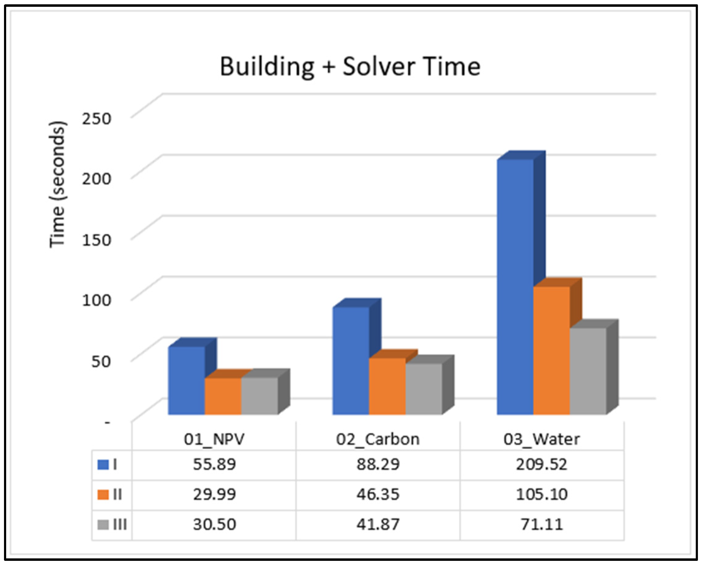
Overall, combining building and solver times, Model III emerges as the more efficient model in all scenarios, with its relative performance improving with scenario complexity. As depicted in Figure 4, Model III matches Model II in Scenario 1 but is more efficient in Scenarios 2 and 3, taking only 90% and 67% of the Model II solution time, respectively. It should be acknowledged, however, that solution time may be more critical than building time when it is necessary to solve more-or-less the same problem many times, such as when one wishes to compare slightly different scenarios or to find the Pareto frontier with a multi-objective problem.

We broke down the building times into finer categories to better understand the results. Table 6 breaks down the building time for Scenario 3, showing the duration of each model-building step. The look-up tables are necessary for linking decision variables to nodes and establishing node connections (i.e., building the sets and functions described in Section 2.2 to 2.4). This step consumes more time in Model III due to the larger number of variables and connections. This is also reflected in the “Conservation of Area Declaration,” where Model I has fewer rows than Model II, and Model II has fewer than Model III (Table 4). Because Model III also requires more decision variables (linear programming columns) than Models I and II (Table 4) set declaration times are also longer. However, the time for declaring other sets (periods, ages, sub-regions, management units) is relatively minor. The time for parameter declaration is consistent across models, as parameters are indexed identically by node for all models.

Table 6 shows that building the accounting constraints consumes the majority of the time to build Scenario 3 formulations, in fact, for Model I, writing the PltCover accounting constraints takes more than half of the total model building time. The time to build these constraints is longest for Model I and shortest for Model III, with Model II generally taking about twice as long as Model I and Model III generally taking about twice as long as Model II. These results show the efficiency of Model III for handling accounting variables. This efficiency is especially critical when dealing with complex accounting variables like PltCover that require accounting across multiple indices (e.g., both periods and micro-watersheds).

Table 6 shows that once accounting constraints and corresponding accounting variables are established, the time required to declare ‘Constraints’, ‘Objectives,’ and ‘RHS’ is minimal, under 0.005 seconds for all models.

Figure 1, Figure 2, and Figure 3 illustrate why the accounting constraint construction process is so much more efficient with Model III. There is one of nonzero coefficient in each accounting constraint for each node in the figures. In Models I and II, nodes are duplicated across multiple variable paths. Because nodes are not duplicated in Model III, there are fewer non-zero coefficients in the accounting constraints. Table 7 shows the number of non-zero coefficients for each accounting constraint set in this study for each model type. Except for the VolCut accounting constraints, Model II has less than half the number of non-zero coefficients compared with Model I, and Model III has less than half the number of non-zero coefficients compared with Model II. In fact, except for the VolCut accounting constraints, Model III has less than one fifth of the non-zero coefficients that are required in Model I.

To gain insight into the solver phase, we examined Gurobi’s presolve report. Gurobi’s presolver simplifies the optimization problem through problem size reduction, bound tightening, and identifying unique structures. Table 8 summarizes key presolve metrics for each scenario, illustrating Gurobi’s effectiveness in simplifying and significantly reducing the size of all three models.

In Scenario 1, Gurobi’s presolve process results in Models II and III having an equal number of rows, columns, and nonzeros, suggesting that the two models are structurally similar, if not equivalent, in this case. In this case, the difference in the solution times for these models can be attributed to the presolve time, not the actual solution time. However, in Scenarios 2 and 3, Model III maintains more columns and rows than Model II after the presolve process. These differences are relatively small, however, suggesting that both models still converge towards very similarly structured problems. More importantly, after the presolve process, Model III has noticeably fewer nonzeros than Model II in these scenarios – roughly one third and one half in Scenarios 2 and 3, respectively.

Conversely, while the presolver results in Model I having fewer columns and dramatically fewer rows in all scenarios, compared to Models II and III, Model I consistently has more nonzero coefficients. Finally, the density of the Model I and Model II matrices increases faster than the density of the Model III matrices as model complexity increases. After presolving, there are approximately six times more nonzeros in both Models I and II for Scenario 2 vs Scenario 1, while the number of nonzeros increases by a factor of less than four for Model III. Similarly, between Scenario 2 and Scenario 3, the number of nonzeros increases by a factor of 2.7X for Model I, 2.2X for Model II, and 1.9X for Model III. These differences in constraint matrix densities are likely a key reason why Model I has the longest solution times in spite of having fewer variables and constraints. In addition, Gurobi’s presolver likely recognizes the network structure inherent in Models II and III, enabling more effective application of cutting planes to expedite the solution process [75].

4. Discussion and Conclusions

This paper revisits the Model I, II, and III formulations of the forest management planning problem. Depending on one’s previous understanding of the three models, one might say that we have redefined Models II and III. The paper shifts the focus in defining these formulations away from whether areas can be merged into combined management units after stand-replacing harvests. Rather, it focuses the definitions of the different models on the sequences of management unit states represented by the variables. In Model I, variables represent a complete sequence of states from the beginning of the planning horizon to the end. In Model II, variables represent a sequence of states from one management intervention to the next. Finally, in Model III, variables represent a single arc in the decision tree for a management unit, representing only two states: a beginning state and an ending state.

While it is possible in Models II and III – and not in Model I – to merge areas into combined management units so they can be represented by a single set of variables following a stand-replacing harvest, we suggest that this is not the critical distinction between the models. In fact, we have mostly ignored this possibility in this paper, and we do not take advantage of this option in our analysis. It is possible that allowing for the merging of similar areas into combined management units following a management-unit-replacing harvest would result in even greater efficiencies for Models II and III, but we leave this question for future research. The option of merging management units is also less attractive in the case of spatially explicit models, since in those models all management units differ in terms of their locations. In addition, because we do not consider the option to combine areas following a complete harvest, we do not differentiate between stand-replacing interventions and other interventions. If one wishes to merge management units following final harvests, then this distinction is crucial, and the models will be more complex than the ones presented here.

Not surprisingly, given our definitions, Model III has the most variables and constraints, Model I has the fewest, and Model II is somewhere in between. In past studies, such as Johnson and Scheurman [41], the focus of Model II was on the possibility of reducing the number of variables through the merging of management units. However, our analysis indicates that the number of variables and constraints is not strongly related to model formulation time and even solution time. In fact, our analysis suggests that the density of the parameter matrix is a key metric that past studies have ignored, and in this regard, Model I have the densest parameter matrix, and Model III has the least dense matrix. This difference in parameter densities is driven largely by the construction of accounting constraints. Thus, as models include more accounting constraints for an increasing array of ecosystem services, the advantages of Model III become more apparent.

Our analysis indicates that Model III’s efficiency advantage over Model I increases with the number of ecosystem services (ES) considered, and the solution time advantage of Model II vs Model III decreases with the complexity of the problem. These trends are linked to the computational demands of incorporating each ES. A corresponding set of accounting constraints must be constructed for every ES included in the model. The computational load intensifies since ES considerations can apply to every alternative across all periods and the entire horizon. Models I and II, which frequently represent the same state (node) in Figure 1 with multiple variables, require greater formulation time and a denser parameter matrix. In terms of solution time, Model II performs somewhat better than Model III in our case study, but the difference between the solution times of Models II and III is less than the difference between Models III and I. Furthermore, the differences decrease as the number of ESs in the model increases.

Our results are based on a single case study. Further research is needed to explore Model III’s adaptability to various problem structures. This includes testing its performance with different numbers and configurations of alternatives per management unit, leading to varying tree-graph shapes and consequent impacts on efficiency. Model III’s robustness should also be assessed in scenarios involving binary decision variables, adjacency, transportation constraints, and stochastic models.

Additionally, it is crucial to evaluate building and solver times independently for researchers and practitioners implementing forest planning models in contexts such as Monte Carlo simulations, Pareto Frontier calculations, or any iterative process using a persistent solver. Given the varying demands of controlling numerous ES, the performance differential can be significant.

In our analysis, Model I consistently underperformed the other models in both building and solving times across all scenarios. All three model formulations have been around for nearly half a century, so it is somewhat curious that most practitioners have adopted the Model I approach. Model I’s widespread usage might be attributed to its matrix approach, which aligns well with the familiar spreadsheet format. This alignment extends to the design of linear programming problems, where variables and constraints correspond to columns and rows, respectively, facilitating intuitive program development for solver submission. Or the preference for Model I could be due to its more compact formulations, with fewer variables and fewer constraints. However, as our results demonstrate, these metrics of model size and complexity may not be good predictors of model formulation and solution times. In contrast, Models II and III, which employ network concepts, can be perceived as more complex and challenging to understand and teach. Network-based models, while frequently discussed in forest management literature, have yet to see widespread adoption among researchers and practitioners, possibly due to the abovementioned complexities. However, they are favored in commercial software owing to typically superior performance. Models II and III demand a network format for alternative generation, requiring advanced programming skills beyond the matrix approach. Nevertheless, it is possible that the decision-tree structures of Models II and III may ultimately be easier to understand for users who have not already been indoctrinated with the matrix-based perspective of most linear programming models. For us, at least, Model III is conceptually straightforward if one visualizes the forest management problem as a decision tree – a sequence of decisions as shown in Figure 1 – rather than as a matrix.

Model III emerges as a promising alternative, offering enhanced performance and greater accessibility in terms of understanding and programming. Unlike Models I and II, Model III adopts a perspective centered on forest states, viewing forests as ES sources subject to human interventions designed to achieve target future forest states. This approach could potentially resonate more naturally with researchers and practitioners, simplifying the process of programming management alternatives and building models. In addition, because Model III has a variable representing the state of each management unit at each point in time, it is well suited to introducing uncertainty into the model formulation. This likely explains why authors such as Eriksson [58], Reed and Errico [22] and Davis and Martell [54] found Models II and III to provide a superior framework for incorporating uncertainty. At the very least, we hope this paper gives forest management planners new reasons to reconsider both Models II and III, rather than the ubiquitous, yet plausibly inferior, Model I.