
Submitted:
15 July 2024
Posted:
16 July 2024
You are already at the latest version
Abstract
Since the 1960s, forest planners have used linear programming models to develop management plans for large, forested areas. Hundreds of academic papers have presented such models, incorporating multiple objectives, a growing diversity of management interventions, and uncertainty, among other things. Three basic ways to formulate these models have been used: Model I, III, and III. We define these models based on the sequence of management unit states represented by the variables. In Model I, variables represent a sequence of states from the beginning of the planning horizon to the end. In Model II, variables represent a sequence of states from one intervention to the next. Finally, in Model III, variables represent a single arc in a management unit’s decision tree, including only a beginning and an ending state. We formulate each type of model for a case study with three increasingly complex scenarios incorporating additional ecosystem services. Our results indicate that, despite requiring more variables and constraints, Model III requires the least time to formulate, largely because it has the least dense parameter matrix. Model II has the shortest solution times, with Model III close behind. Model I requires both the longest formulation and solution times.
Keywords:
forest management
; strategic planning
; harvest scheduling
; ecosystem services modeling
1. Introduction
Linear programming (LP) has been used to support forest management planning since the [1,2,3,4,5,6]. Many variations of these models have been proposed, including, for example, multi-objective models [7,8,9,10,11,12,13,14], spatially-explicit mixed integer programming (MIP) models [15,16,17,18,19,20], and models incorporating uncertainty [21,22,23,24,25,26,27]. While earlier forest planning LP models often considered only one type of management intervention – final harvest and regeneration of even-aged management units – since at least Randall [28], analysts have been incorporating a variety of other interventions – such as thinning [28] and coppice harvests [29]. These models originally focused on scheduling timber harvests in even-aged forests to maximize harvest volumes or net present values, but today these models’ management objectives include a diverse range of ecosystem services [14,30,31]. Multiple demands on forests for a variety of products and services have led to the development of multifunctional forestry planning models that account for timber and non-timber values and services, such as berry and mushroom picking [32], carbon sequestration [33,34,35,36], habitat sustainability, deadwood availability, carbon storage [37,38], biodiversity conservation indicators [39], and hunting benefits [40].
Johnson and Scheurman [41] formalized two fundamental ways to formulate LP models of the forest management planning problem, which they named Model I and Model II. Other authors [22,42,43,44] have used a third formulation that has been referred to as Model III [45,46]. While hundreds of papers have been written about LP and MIP forest planning models, most models described in the literature have used Model I [47]. We have found only a few articles that use Model II. Nanang and Hauer [40] use Model II to build a model exploring tradeoffs between timber production and hunting benefits; Diaz-Balteiro et al. [48] present a special harvest scheduling model for a community forest; and Grossberg [49] integrates road access to harvest scheduling. While not strictly an LP model, Sessions et al. [50] use simulated annealing to solve a harvest scheduling model with spatial control whose design is based on Model II. However, at least two forest management software packages used for industrial and agency applications at least give the option of using Model II. Woodstock Optimization Studio [51] a forest planning application widely used in the forest products industry, and PRISM [52], a U.S. Forest Service application, both allow Model II formulations. We have identified relatively few articles that use Model III [22,42,43,53,54]. Salo and Tahvonen [44] list Model II in their key words, but their model is better described as Model III.
There often are multiple ways to formulate any given real-world problem as a mathematical model. When different formulations all produce the same solution, it is useful to assess the advantages and disadvantages of the different formulations, and whether it matters at all which formulation is used. A few papers have compared the relative performance of Model I vs. Model II. Johnson and Scheurman [41], who introduced Model II, focused on model size and solution time in the context of large LP models, which in 1977 were resource-intensive to formulate and solve given the computing capacity of the time. Their concern with model size led them to focus on the possibility of combining analysis areas that differ only in their initial age class after a clearcut harvest (since the initial age class is no longer relevant). Barros and Weintraub [55] also focus on the ability to reduce the number of variables in Model II by combining similar management units when they are harvested in the same period. Today, however, model size is seldom a significant concern for non-spatial LP models. However, model size and solution time is (and probably always will be) a concern for spatially explicit models, which generally involve binary variables [16]. However, in spatially explicit models all management units differ in terms of their location, so combining management units removes the ability to model a management unit’s locations. McDill et al. [56] and Martin et al. [57] compared Model I and Model II formulations in the context of MIP planning models, focusing primarily on solution time. These papers came to opposite conclusions, with McDill et al. [56] finding that Model II performed better and Martin et al. [57] giving the advantage to Model I. Eriksson [58] compared Model I and Model II in the context of modeling uncertainty and concluded that Model II more easily accommodates a stochastic approach and produces smaller stochastic models due to its tree-graph design instead of the matrix design of Model I. Reed and Errico [22] take advantage of the structure of Model III for addressing uncertainty related to fire. Based on these few studies, it is difficult to determine whether one formulation is superior for any given application, and one might conclude that perhaps no formulation will consistently outperform another.
Additional criteria could also be considered when comparing different model formulations, including how easy they are to understand and the insight they provide into the structure of the real-world problem being modeled. For example, Model I might have been used more than Model II because it is easier to understand, or because it fits more naturally into the matrix-based structure of a LP model, or even simply because more papers use it and that is the formulation most analysts are familiar with. Especially for large models, storage considerations and model formulation time may also be important. In any case, unless one formulation is uniformly superior to another, having multiple ways of formulating a mathematical model is generally a good thing since one formulation may work better for one situation while another formulation works better for another problem.
This paper revisits Models I, II, and III and considers them from a new perspective. We present the three model formulations using a consistent notation that illustrates the similarities and differences between them. Our presentation of the models shows the matrix perspective underlying Model I, and the network – or decision tree – perspective underlying Models II and III. This difference has also been noted by Garcia [42] in the case of Model III, and Erickson [58] in the case of Model II. Additionally, we suggest that while Model II has a network structure, it has an intervention-focused perspective, while Model III reflects a state trajectory perspective. This state-focused perspective can be particularly useful when the problem involves objectives or constraints, such as water yields, forest carbon storage, and other ecosystem services that depend on the state of the forest at any given time, rather than the inputs and outputs that result from interventions. Most applications of Models II and III have considered final harvest to be the only type of intervention. Garcia [42] discusses the possibility of thinning, but thinning was not included in the actual model described in that paper. Our presentation of these model formulations allows any type of intervention.
We believe there has been some ambiguity in the specific definitions of the Model I, II, and III formulations, which we hope this paper will resolve. Several papers [41,42,55] have emphasized the possibility of combining management units after clearcutting, which is possible with both Models II and III but not with Model I. In fact, Gunn [46], Martin et al. [57], and Nguyen et al. [52] require (as part of the definition of these models) the merging of management units that differ only in their age when they are regeneration harvested in the same planning period. But we propose an alternative definition of these models that does not identify this as the salient difference between the three model formulations. Our definition differentiates the models based solely on the sets of periods represented by the model variables. Thus, by our definition:
In Model I, a variable represents the state of the area assigned to it for an entire sequence of states, interventions, and non-interventions covering the entire planning horizon of the model. In Model II, a variable represents the area assigned to it for one of three sets of periods: 1) the set of periods between two interventions, 2) the set of periods from the initial state to the first intervention, or 3) the set of periods from the final intervention to the end of the planning horizon. In Model III, a variable represents the state of the area assigned to it for one pair of adjacent periods.
Note that we use the term “intervention” in a very general sense here. Alternatively, a variable in Model II could be defined as representing the area assigned to it for the set of periods 1) between two stand-replacing interventions (e.g., regeneration harvests), 2) from the initial state to the first stand-replacing intervention, or 3) from the final stand-replacing intervention to the end of the planning horizon. This is, in fact, the traditional definition used by, among others, Gunn [46], Martin et al. . [57], and Nguyen et al. [52]. This version could, perhaps, be called Model IIB, while our definition could be called Model IIA. This distinction is moot when regeneration harvests are the only interventions considered, as is often the case. It is perhaps less confusing to use Model IIB when the emphasis is on merging similar areas after regeneration harvests (as do Gunn [46], Martin et al. [57], and Nguyen et al. [52]). However, when one has a variety of interventions, including some that are not regeneration harvests (e.g., thinning), Model IIB becomes more complex, as in many cases there will be more than one sequence of interventions between any two regeneration harvests. Model IIA can accommodate merging similar areas after regeneration harvests, but one would have to differentiate between stand-replacing interventions and other interventions. We do not consider this possibility in this paper because it would complicate the exposition and possibly perpetuate confusion and ambiguity in the definitions of the three model formulations.
After we review the structure of the three formulations, we compare the size and performance of Model I, II and III formulations in the context of a case study of strategic planning in the management of a eucalyptus plantation problem in Brazil. Our intent is not to demonstrate that any of the model formulations are necessarily superior for all problem instances. Rather, the example is intended to illustrate the differences in model size, formulation time, and solution time and when and how different formulations might be preferred. We do not evaluate the performance of the different model formulations in the context of spatially explicit MIP formulations of the forest ecosystem management planning problem.
2. Methods
This section consists of three parts. Section 2.1 to Section 2.4 specify our formulation of Models I, II, and III. Figure 1, Figure 2 and Figure 3 use decision trees for a single example management unit to illustrate the structure of the three models, emphasizing the differences and similarities in each model’s decision variable definitions, area conservation constraints, and accounting constraints. Particular attention is paid to modeling ecosystem services in harvest scheduling models, as the advantages of the Model III formulation are more apparent when multiple ecosystem services are modeled.
Section 2.5 and Section 2.6 describe a real-world forest ecosystem management problem involving a 12,732-hectare industrial eucalyptus plantation in São Paulo, Brazil, comprised of 350 management units. This forest area is managed primarily to provide pulpwood for a nearby mill, but other ecosystem services, including carbon sequestration and water conservation are considered. This example problem will be used to conduct a comparative analysis of the three model formulations in the context of three scenarios, each incorporating an additional ecosystem service.
Section 2.7 details the experimental setup, including computational resources, solver specifications, and the methodology for running and evaluating the scenarios. It also identifies the performance metrics used to compare the models.
2.1. Example Decision Treee Graph Representation for a Single Management Unit
It will be useful to consider how the variables in each model represent the management alternatives for a single example management unit as we describe the three forest management model formulations in the coming sections. The alternatives for this example unit are presented as a decision tree in Figure 1. The figure contains three types of nodes: the initial node (brown), non-intervention nodes (gray), and intervention nodes (red, blue and green). We do not differentiate between stand-replacing interventions and non-stand-replacing interventions. The specific nature of the interventions is not critical for the example (or for our model definitions), but when the possibility of an intervention exists, the decision tree branches to represent the decision to either implement the intervention (represented by an intervention node) or not (represented by a non-intervention node). Thus, for example, in period 2 there is a decision to either conduct an intervention (node 3 in Figure 1) or not (node 18 in Figure 1).
For each model, we first define the sets, variables and parameters needed to formulate the model and then we give the equations of the model. Alternative equations for a spatially-explicit model are presented following each non-spatially-explicit model formulation. Analogous equations for spatially-explicit models are given the same number, and a prime symbol indicates that an equation is for the spatially-explicit model. As we introduce new models, sets, variables and parameters that have been defined for previous models are not repeated. Table 1, following the presentation of the models, lists the sets for each model for the example networks shown in Figure 1, Figure 2 and Figure 3.
2.2. Model I Formulation
In Model I, each variable represents a complete management alternative for a management unit for the entire planning horizon. Figure 2 illustrates this by representing the management alternatives from Figure 1 as separate sequences of nodes for each complete management prescription. For example, the first prescription is represented by the sequence {1, 2, 3, 4, 5, 6, 7, 8}, and the second prescription is represented by the sequence {1, 2, 3, 4, 9, 10, 11, 12}. In a non-spatially-explicit model, the variable would represent the area of unit u where prescription 1 would be applied. In a spatially-explicit model, the variable would take a value of one or zero, representing, respectively, whether prescription 1 would be applied to unit u or not. The number of Model I variables for a given management unit equals the number of ending nodes in that unit’s decision tree graph.
2.2.1. Sets
set of economic quantities, ecosystem services, or landscape conditions (e.g., costs, revenues, timber harvests, timber inventory, carbon stocks or flows, old growth, recently clear-felled area, etc.). For brevity, we will refer to any of these items simply as ecosystem services.
set of management units.
set of time periods {min{-tfu}, …, 0, 1, 2, …, T}; -tfu represents the time of the most recent (past) intervention for unit u.
set of nodes for unit u.
set of nodes for unit u in a general period t; is a subset of .
the set of nodes for unit u in the specific period T (the last period); these are called “ending nodes.”
set of prescriptions for unit u (the term “prescription” is used here to mean a management plan for a single management unit from time 0 to period T, as represented by a connected sequence of nodes from t=0 to T).
Note: there exists a one-to-one mapping from each ku to each .
sequential (ordered), connected set of nodes for unit u that represent prescription ku .
node for unit u in prescription ku for period t (note: there is only one for period t in prescription , but a node may belong to more than one prescription).
2.2.2. Variables
equals the quantity of ecosystem service e provided in period t.
Non-spatially-explicit model:
equals the area of unit u on which prescription ku will be applied.
Spatially-explicit model:
equals 1 if prescription ku is applied to unit u, 0 otherwise.
Because there is a one-to-one mapping from each ku to each there is one variable for each . For the management unit in Figure 1, there will be eight variables.
2.2.3. Parameters
the contribution of node to ecosystem service e in period t. Note that is stored in the prescription database with the node . In the non-spatially-explicit model, these values are expressed on a per-unit of area basis; in the spatially-explicit model, they are expressed on a per-management-unit basis.
objective function preferential weight for ecosystem service or landscape condition e in period t. For all models it is assumed that .
the area of unit u.
2.2.4. Formulation
Model I for a non-spatially-explicit forest management problem can now be written as follows:
Subject to
Equation (1) defines the objective function as a weighted sum of the economic values, ecosystem services, and landscape conditions produced in each period. Equation set (2) is the set of area constraints; they state that the sum of the areas from unit u assigned to each prescription must equal the area of unit u. Equation set (3) is the set of accounting constraints for each ecosystem service for each period. Equation (4) states that the sum of the objective function weights equals one. Equation sets (5) and (6) are non-negativity constraints for the model variables.
For a spatially-explicit model, replace Equation set (2) with Equation set (2’) and Equation set (5) with (5’), as follows:
Equation (2’) states that one and only one prescription can be applied to unit u, and Equation (5’) states that the X-variables are binary, i.e., they must equal either zero or one.
Upper or lower bounds on the values or changes in the values of the ecosystem service accounting variables can easily be added to the base model represented by Equations (1) to (6). For example, one could add constraints enforcing minimum or maximum harvest levels, minimum or maximum carbon stored in the forest, minimum levels of carbon accumulation, maximum area of cleared forest within a given zone, minimum area of forest older than a given age, maximum change in the harvest level between periods (flow constraints), etc. The possibilities are too numerous to describe them all here. Adjacency constraints, accessibility constraints, etc. can also be added to the spatially-explicit model. Again, enumerating the possibilities is beyond the scope of this article. It should be noted that a well-constructed model should include constraints on either the ending state of the forest (target forest conditions) and/or include appropriate values for possible ending states in the objective function to ensure accurate valuation of the forest resource and the sustainability of the forest beyond the planning horizon [59].
2.3. Model II Formulation
In Model II, each variable represents the state of the area or management unit assigned to it for a period of time (sequence of nodes) that begins either at the beginning of the planning horizon or immediately following a management intervention and that ends either with an intervention or at the end of the planning horizon. Figure 3 illustrates this by representing the alternatives from the example in Figure 1 as they would be represented in Model II. For example, the first variable would represent the sequence {1, 2, 3}, and the second and third variables would represent the sequences {3, 4, 5} and {3, 4, 9, 10}, respectively. In Model II, the number of variables for a given management unit will equal the number of interventions that can be applied to that unit plus the non-intervention ending nodes in that unit’s decision tree graph. Equivalently, the number of variables equals the number of intermediate intervention nodes (defined below), plus the number of ending nodes.
2.3.1. New Sets
the initial node for unit u.
set of intermediate intervention nodes for unit u; these are nodes that represent an intervention, excluding the initial node (if it is an intervention node) and any intervention nodes that occur in period T; this is why this set is referred to as “intermediate” intervention nodes.
set of intermediate non-intervention nodes for unit u; this set includes all non-intervention nodes except the initial node (if it is a non-intervention node) and any non-intervention nodes that occur in period T.
Note that the set can be partitioned into four sets: .
A “prescription” in this model is a sequence of nodes that starts with either the initial node, , or an intermediate intervention node, , and ends with either an intermediate intervention node, , or an ending node, . Again, let
set of prescriptions for unit u.
set of nodes that represent the last node in a prescription.
Note that the set in Model II is different from the set in Model I. Assuming we are not merging similar areas after regeneration harvests, there is a one-to-one mapping from each prescription to each . Otherwise, there would be a many-to-one relationship between prescriptions in and nodes in . In our examples, we did not merge similar areas after regeneration harvests.
Define the function as returning the prescription that ends at node .
For each node there is a set of prescriptions that start with node . Define the set:
as the set of prescriptions that that start with node .
Similarly, define the set:
as the set of prescriptions that start with intermediate intervention node (where j is the index to the set corresponding to the intermediate intervention node ).
Define the function that returns the index j for the set corresponding to the intermediate intervention node .
set of prescriptions for unit u that contain a node in period t.
2.3.2. Variables
The variables in Model II have definitions like those in Model I. What has changed is the prescriptions (sequence of nodes) that they represent.
Non-spatially-explicit model:
equals the area of unit u on which prescription ku will be applied.
Spatially-explicit model:
equals 1 if prescription ku is applied to unit u, 0 otherwise.
2.3.3. Parameters
The parameters are the same as for Model I.
2.3.4. Formulation
Model II can now be written as follows:
Subject to
Equations (1), (4), (5), and (6) are the same as for Model I. Equation set (7) is analogous to Equation set (2) from Model I, but the summation on the left-hand side is only over the prescriptions that start from the initial node. Equation set (8) are network flow conservation constraints stating that the total area entering an intermediate intervention node must equal the total area leaving the node. Equation (9) is very similar to Equation (3); the only thing that has changed is that we only sum over the set of variables that contain a node in period t.
For a spatially-explicit model, replace Equation set (7) with Equation set (7’) and Equation set (5) with (5’), as follows:
As with Model I, upper or lower bounds on the values or changes in the values of the ecosystem service accounting variables can easily be added to the base model. Adjacency constraints, accessibility constraints, etc. can also be added to the spatially-explicit model. Again, a well-constructed model should include constraints and/or objective function coefficients that ensure accurate valuation of the forest resource and the sustainability of the forest beyond the planning horizon [59].
2.4. Model III Formulation
In Model III, each variable represents a sequence of two nodes that starts with either the initial node, , or an intermediate node, , and ends with either an intermediate node or an ending node, . Figure 1 represents Model III, where each node represents a forest state. Note that each variable corresponds to an arc in the network representation in Figure 1. In Model III, the number of variables for a given management unit would equal the number of nodes in that unit’s decision tree graph, excluding the initial node; for the example in Figure 1, this would result in 31 prescriptions.
2.4.1. New Sets
set of all intermediate nodes (intervention plus non-intervention) for unit u (the “c” superscript indicates that is a combination of and ).
Now, the set can be partitioned into three sets: A “prescription” in this model is a sequence of two nodes that starts with either the initial node, , or an intermediate node, , and ends with either an intermediate node, , or an ending node, . Now, let
set of prescriptions for unit u.
Note that the set in this model is different from the sets in Model I and in Model II. In this model there is a one-to-one mapping from each prescription to each . As with Model II, it is possible to merge similar areas after regeneration harvests; if this was done, there would be a many-to-one relationship between prescriptions in and nodes in .
Define the function as returning the prescription that ends at node .
For each node there is a set of prescriptions that start with that node (). Define the set:
as the set of prescriptions that that start with node .
Similarly, define the set:
as the set of prescriptions that start with intermediate node (where j is the index to the set corresponding to the node ).
Define the function that returns the index j to for the set corresponding to the intermediate node .
set of prescriptions for unit u that end with a node in period t.
2.4.2. Variables
The variables in the model are again either.
Non-spatially-explicit model:
equals the area of unit u on which prescription ku will be applied.
Spatially-explicit model:
equals 1 if prescription ku is applied to unit u, 0 otherwise.
2.4.3. Parameters
The parameters are the same as for Model I and II.
2.4.4. Formulation
Model III can now be written as follows:
Subject to
Note that this model is virtually the same as Model II. The only difference is Equation Set (10), which is analogous to Equation Set (8) except that we now have one equation for each intermediate node (not just for intermediate intervention nodes) each management unit. This, and the number of nodes represented by the variables, is the only difference between Models II and III.
As with Model II, for a spatially-explicit model, replace Equation set (7) with Equation set (7’) and Equation set (5) with (5’), as follows:
2.5. The FEM Problem Description
We created a case study of a management problem for an area of fast-growing eucalyptus plantations owned by an integrated forest products company in São Paulo, Brazil to compare various attributes of Models I, II, and II. The plantations in the case study are managed using a short-rotation coppice and renewal regime with the primary objective of pulpwood production. The plantation, comprising 350 management units over 12,732 hectares, employs clear-cuts followed by renewal (CCR) or sprouting (coppice) from stumps (CCS) at ages 6, 7, and 8 years, extending to 11 years in the first three periods for older management units. This regime aligns with regional practices, allowing only one CCS before a mandatory CCR.
We calculated the inventory, harvest volume, and current annual increment (CAI) for three site indexes (23, 26, 29 m) using yield curves provided by the company. The mean average increments at age seven (MAI7) are 26.96, 31.40, and 36.73 m3/haꞏyear in the first rotation and 22.92, 26.69, and 31.22 m3/haꞏyear in the second rotation for the three site indices, respectively.
Genetic material, mostly Eucalyptus grandis, Eucalyptus urophylla, or their hybrids, were grouped by basic wood density (BWD) properties into four categories that influence carbon sequestration calculations. The high, medium, low, and very low-density groups range from 0.463 to 0.531, 0.446 to 0.503, 0.403 to 0.488, and 0.355 to 0.481 t/m3, respectively, depending on the stand age.
The company provided the initial state of each management unit, including location (region, sub-region, and site index), genetic material, area, last intervention time, and type. A 21-year planning horizon, divided into one-year planning periods, was used, reflecting three average rotations.
Carbon sequestration calculations were based on Sanqueta et al. [60], utilizing the Biomass Expansion Factor (BEF), Root Shoot Ratio I, and Biomass Carbon Fraction Factor (BCF). We used data from the same species collected in a similar region from Ribeiro et al. [61]. We obtained the factors BEF = 1.2220, R = 0.1689, and BCF = 0.4323, which are ratios with no units.
Additionally, the company reported natural forest coverage per subregion, maintaining at least 20% to meet Brazilian regulations. We use sub-regions as a proxy for micro-watersheds to calculate water-related ecosystem services (ESw). There is a threshold of 20% of natural forest coverage in a micro-watershed with eucalyptus plantations, below which ESw supply tends to become unsustainable and a desirable level of 45% for the highest ESw gains [62]. These data, with concepts from Lima and Zakia [63], are used in our third scenario that considers ESw, as described in more detail below.
Production costs were provided per region in BRL (Table 2; BRL = Brazilian reais, also represented by R$). A conservative interest rate of 6% was chosen to avoid biasing the model towards early harvesting [64,65]. The pulpwood price, R$ 100.00, is typical for the region. We used a social value of carbon as a proxy for the carbon value, which is R$ 120/t of CO2 in Brazil [66,67].
We calculated terminal values (TV) following the methodology outlined by Kanieski da Silva et. al. [59], accounting for regional cost differences and production variations specific to each region and site index. This involved initially determining a management regime that maximizes the Land Expectation Value (LEV) for each region and site index (Table 3) and then calculating a Forest Value [68] by age, region, and site assuming this management regime would be followed in perpetuity.
All values, tables, and assumptions from this section, including the initial state by management unit, genetic material BWD, required forest cover per sub-region, production tables, costs, LEV, TV for each potential ending condition, formulas, and a Visual Basic macro for TV calculations, are provided in the supplementary material. These data are compiled in an Excel® spreadsheet titled “Assumptions.xlsm,” along with detailed carbon calculation methodologies.
Lastly, we utilized iGen by Romero® [69] to generate all possible management alternatives for this FEM problem. iGen produced a tree graph similar to Figure 1 for each management unit, resulting in a total of 426,191 nodes for all management units. It calculated a suite of parameters for each node for use in formulating the linear programming models, including age, inventory, harvest volume, discounted revenue and costs, carbon sequestration, forest cover, and an age control indicator for the ESw scenario. Additional variables maintained during alternative generation, such as region, sub-region, management unit, area, site index, period, intervention type, rotation, and genetic material, along with the rules and equations of motion, are detailed in an Excel® spreadsheet “Alternatives.xlsx,” available in the supplementary material.
For this study, the node data were read to build non-spatial Models I, II, and III according to the formulations presented in the previous sections. While Section 2.2, Section 2.3, and Section 2.4 describe both non-spatial and spatially-explicit versions of their respective models, including spatially-explicit versions of the case study models was beyond the scope of this analysis. In addition to a base case that considers only the profitability of timber production, two additional scenarios were considered with each scenario adding additional management objectives (ecosystem services). These scenarios are detailed in the following section. Each scenario was formulated using Model I, II and III, resulting in a total of nine LP formulations.
2.6. Scenarios Description
This study hypothesizes that Models I, II and III perform differently when managing for an increasing number of Ecosystem Services (ES). To examine this, we have structured scenarios with escalating complexity. Scenario 1 is a standard timber production harvest scheduling model that presents a baseline case. Scenario 2 adds carbon sequestration as an additional ES management objective to Scenario 1. Finally, Scenario 3 adds an additional water-related Ecosystem Services (ESw), thus providing the most comprehensive and complex scenario for analysis.
2.6.1. Scenario 1 – Harvest Scheduling
Scenario 1 focuses on timber production, including timber revenue, the costs of silviculture activities, and the terminal value. The objective function was to maximize the Net Present Value (NPV), which includes the sum of discounted timber management net revenue and the terminal value. The model includes flow constraints allowing ±5% production variation starting from period four. The flexibility in the first three years, during which harvests in older ages are allowed due to existing older management units, provides an adjustment period before imposing flow constraints.
The parameters necessary for this scenario – VolCut (volume of timber cut), DscTmbCst (discounted timber costs), and DscTmbRev (discounted timber revenue) – were calculated using iGen, as detailed in the previous section. During model-building phase, we used these parameters to define three corresponding sets of accounting variables by period. The VolCut accounting variables were required to establish the flow constraints, while DscTmbCst and DscTmbRev were utilized to compose the NPV objective function.
2.6.2. Scenario 2 – Carbon Analysis
In Scenario 2, we expanded the model to include carbon sequestration and its associated value. A new parameter, CRemoved (carbon removed from the atmosphere), was introduced and calculated by iGen, as detailed previously. CRemoved quantifies the CO2 in tons per hectare removed from the atmosphere and fixed in the trees’ biomass (both above and below ground) during the current period. In this scenario, the revenue parameters, which previously included only timber revenues and terminal values, were adjusted to include the value of carbon sequestration, obtained by multiplying the amount of carbon removed by the social cost of carbon. Similarly, the cost parameter was adjusted to account for carbon emissions resulting from harvesting, calculated by multiplying the carbon content in the harvested volume by the social cost of carbon. Additionally, we introduced a new set of constraints to ensure non-declining carbon sequestration, stipulating that CRemoved must not decrease over time. The objective function remains the Net Present Value (NPV), which now integrates the carbon value into the revenue and cost components.
The harvest flow constraints from Scenario 1 were also included in this model. Thus, the parameters in this scenario include VolCut (volume of timber cut), DscCosts (discounted costs), DscRevenue (discounted revenue), and CRemoved (carbon removed), used again while building the accounting constraints to compute the corresponding accounting variables, which in turn inform the flow and non-declining carbon constraints, as well as the NPV maximization objective function.
2.6.3. Scenario 3 – Timber, Carbon, and Water
In Scenario 3, we introduced binary parameters, PltCover, to represent the water protection ecosystem service (ESw). PltCover equals 1 when a plantation’s age is two years or older, and 0 otherwise. PltCover is used in a set of accounting constraints to calculate the plantation coverage (the area of soil covered by forest plantations that are at least two years old) within each micro-watershed for each period. Bounds were placed on the resulting accounting variables to set a minimum level of plantation coverage per period in each micro-watershed.
In addition, this scenario incorporated an age control variable to calculate the weighted age by area, computed as the age multiplied by the area represented by each variable divided by the total area (12,732.41 ha) for every period. A set of accounting constraints was added to populate accounting variables to track the average age of the forest per period. A set of non-declining age (NDAge) constraints was added to ensure that this weighted age does not decrease over time because older fast-growing plantation covers are closer to natural forest cover when it comes to improving water-related ecosystem services [63].
Finaly, the scenario retains the constraints from Scenarios 1 and 2, including flow constraints and non-declining carbon. The objective function is the same as Scenario 2, maximizing the Net Present Value (NPV), including the social value of carbon.
2.7. Experimental Setup
iGen by Romero® was used to generate and calculate management alternatives and associated parameters. Data were stored in a remote SQL Server 2022 database [70]. The model-building process for Models I, II, and III was executed through custom software developed in Python [71], utilizing SQLAlchemy [72] and Pandas [73] packages for database connectivity.
Pyomo [74], a Python based algebraic modeling language (AML), was used to construct the optimization models. Pyomo interfaces with the Gurobi Optimizer version 10.0.3 win64 [75] to solve the models. Results and comprehensive control logs detailing each step of the process are saved back to the same SQL Server database. These logs are instrumental for the analysis presented in the results.
All tests were conducted on a local computer equipped with an 11th Gen Intel® Core™ i7-1165G7 CPU @ 2.80GHz, 64GB RAM, featuring four physical cores, eight logical processors, and support for up to eight threads. To ensure the accuracy and integrity of the tests, we turned off all non-essential software to prevent interference with CPU and memory usage. The test suite, encompassing nine runs (three scenarios across three models), was executed in a controlled environment to eliminate the influence of external applications on computing resources.
3. Results
As one would expect, Model I formulations had the fewest decision variables per management unit (240), Model II formulations had an intermediate number (421), and Model III had the most (1,218).
We tracked the time in our analysis of each process phase, from data retrieval from the iGen database to saving the results. Table 4 summarizes the durations of each modeling phase for each scenario and model. Objective function values are shown in the table to confirm that the three models are indeed solving the same forest management problem.
‘Time to Get Data’ is influenced by database organization, database dialect, and internet connectivity rather than model characteristics. This phase shows minimal variance across models and scenarios, attributed to the consistent number of records processed, predetermined by the number of alternatives generated by iGen in an earlier phase. Minor time differences are due to differing parameter sets prepared for the building phase.
Model III requires the least model building time, compared with Models I and II, with this advantage increasing in more complex scenarios. For instance, Model III requires only 38% of building time required for Model I in Scenario 1, and only 27% of the Model I building time in Scenario 3. This is also true, but to a lesser degree, when Model III is compared to Model II.
Model II consistently has the lowest solver time, while Model I requires the largest solver time. However, the difference between Models II and III narrows in more complex scenarios. For example, it takes almost twice as long to solve Model III compared with Model II Scenario 1, while it takes less than 10% more time to solve Model III compared with Model II in Scenario 3. This trend suggests further testing may be needed for more complex scenarios with additional ecosystem services and alternatives.
Overall, combining building and solver times, Model III emerges as the more efficient model in all scenarios, with its relative performance improving with scenario complexity. As depicted in Figure 4, Model III matches Model II in Scenario 1 but is more efficient in Scenarios 2 and 3, taking only 90% and 67% of Model II’s time, respectively. It should be acknowledged, however, that solving time may be more critical than building time when one is solving more-or-less the same problem many times, such as when one wishes to find the Pareto frontier with a multi-objective problem.
We broke down the building times into finer categories to delve deeper into the analysis. For the building process, we detailed the time required for each linear programming element to be provided to the solver. We also analyzed the solver process using Gurobi’s presolve data.
Table 5 breaks down the building time for Scenario 3, showing the duration of each model-building step. The “look-up tables” are necessary for linking decision variables to nodes and establishing node connections (i.e., building the sets and functions described in Section 2.1 to Section 2.4). This step consumes more time in Model III due to the larger number of variables and connections. This is also reflected in the “Conservation of Area Declaration,” where Model I has fewer rows than Model II, and Model II has fewer than Model III (Table 6). Model III also requires more decision variables (linear programming columns) than Models I and II (Table 6), resulting in longer set declaration times. However, the time for declaring other sets (periods, ages, sub-regions, management units) is relatively minor. The time for parameter declaration is consistent across models, as parameters are indexed identically by node for all models.
The notable difference in total building time is clearly due to setting up the accounting variables and their corresponding accounting constraints (Table 5). The need for extensive accounting variables, especially when incorporating ecosystem services over all periods and alternatives, is the reason for Model III’s efficiency. This efficiency is critical when dealing with complex variables like PltCover, which require accounting across multiple indices (period and micro-watershed).
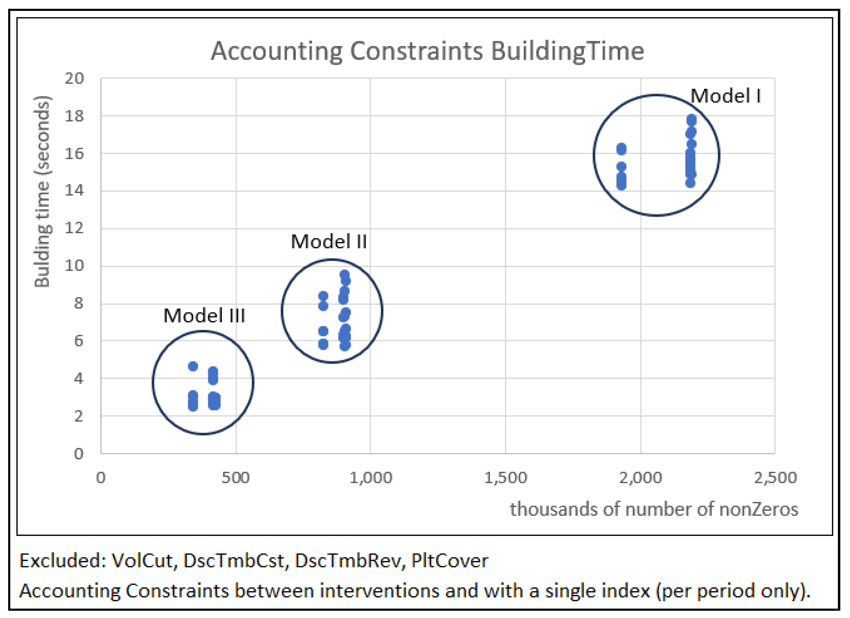
Once accounting constraints and corresponding accounting variables are established, the time required to declare ‘Constraints’, ‘Objectives,’ and ‘RHS’ is minimal, under 0.005 seconds for all models. Understanding the accounting constraint construction process requires analyzing Figure 1, 2, and 3, which illustrate the number of nonzero coefficients involved, essentially one for each node. Table 7 shows the number of non-zero coefficients for each accounting constraint set in this study for each model type. Except for the VolCut accounting constraints, Model II has less than half the number of non-zero coefficients compared with Model I, and Model III has less than half the number of non-zero coefficients compared with Model II. In fact, not counting the VolCut accounting constraints, Model III has less than one fifth of the non-zero coefficients that are required in Model I.
Further tests, including scenario variations, were conducted to develop the graph in Figure 5. Table 7 and Figure 5 show that building time is strongly correlated to the number of nonzero coefficients. These results suggest that the density of the coefficient matrix is an important driver of model formulation time. Detailed measurements from these tests, including accounting constraints results and times, are available in the supplementary material in a spreadsheet named “Results.xlsx.”
To gain insight into the solver phase, we examined Gurobi’s presolve report. Gurobi’s presolver simplifies the optimization problem through problem size reduction, bound tightening, and identifying unique structures. Table 8 summarizes the main presolve metrics for each scenario, illustrating Gurobi’s effectiveness in simplifying and significantly reducing the size of all three models.
In Scenario 1, Gurobi’s presolve process results in Models II and III having an equal number of rows, columns, and nonzeros, suggesting that the two models are structurally similar, if not equivalent. This suggests that the difference in the solution times for these models in this scenario can be attributed to the presolve time, not the solution time. However, in Scenarios 2 and 3, Model III maintains more columns and rows than Model II after the presolve process. Nevertheless, the differences are relatively small, suggesting that both models still converge towards very similarly structured problems. However, Model III still has noticeably fewer nonzeros than Model II in these scenarios – about one third and a half in Scenarios 2 and 3, respectively.
Conversely, while Model I is transformed into a model with fewer columns and dramatically fewer rows in all scenarios, compared to Models II and III, Model I consistently shows a higher count of nonzero coefficients. Finally, note that the density of the Model I and Model II matrices increases faster than the density of the Model III matrices as model complexity increases. After presolving, there are approximately six times more nonzeros in both Models I and II for Scenario 2 vs Scenario 1, while the number of nonzeros increases by a factor of less than four. Similarly, for Scenario 3 vs Scenario 2, the number of nonzeros increases by a factor of 2.7X for Model I, 2.2X for Model II, and 1.9X for Model III. This discrepancy in the density of the constraint matrix is likely one reason why Model I has the longest solution times. In addition, Gurobi’s presolve likely recognizes the network structure inherent in Models II and III, enabling more effective application of cutting planes to expedite the solution process [75].
4. Discussion and Conclusions
This paper presents a new perspective on the Model I, II, and III formulations of the forest management planning problem; depending on one’s previous understanding of the three models, one might say that we have redefined Models II and III. The paper shifts the focus in the distinction among these formulations away from whether areas can be merged into combined management units after stand-replacing harvests. Rather, it focuses on the definitions of the variables in the three models, specifically the sequence of management unit states represented by the variables. In Model I, variables represent a complete sequence of states from the beginning of the planning horizon to the end. In Model II, variables represent a sequence of states from one management intervention to the next. Finally, in Model III, variables represent a single arc in the decision tree for a management unit, representing only two states: a beginning state and an ending state.
While it is possible in Models II and III – and not in Model I – to merge areas into combined management units so they can be represented by a single set of variables following a stand-replacing harvest, we suggest that this is not the critical distinction between the models. In fact, we have mostly ignored this possibility in this paper, and we do not take advantage of this option in our analysis. It is possible that allowing for the merging of similar areas into a single management unit following a management-unit-replacing harvest would result in even greater efficiencies for Models II and III, but this is not the focus of this paper. This option is also less attractive in the case of spatially explicit models, since in those models all management units differ in terms of their locations. In addition, because we do not consider the option to combine areas following a complete harvest, we do not differentiate between stand-replacing interventions and other interventions. If one wishes to merge management units following complete harvests, then this distinction is crucial, and the models will be somewhat more complex than the ones presented here.
Not surprisingly, given our definitions, Model III has the most variables and constraints, Model I has the fewest, and Model II is somewhere in between. In past studies, such as Johnson and Scheurman [41], the focus of Model II was on the possibility of reducing the number of variables through the merging of management units. However, our analysis suggests that the number of variables and constraints is not strongly related to model formulation time and even solution time. In fact, our analysis suggests that the density of the parameter matrix is a key metric that past studies have ignored. Model I has the densest parameter matrix, and Model III has the least dense matrix. Furthermore, the density of the Model III parameter matrix increases less fast than the density of the Model I and Model II parameter matrices as more ecosystem services are included in the model. This difference remains even after Gurobi’s presolve process.
Our analysis indicates that Model III’s efficiency advantage over Model I increases with the number of ecosystem services (ES) considered, and the solution time advantage of Model II vs Model III decreases with the complexity of the problem. These trends are linked to the computational demands of incorporating each ES. A corresponding set of accounting constraints must be constructed for every ES factored into the model. The computational load intensifies since ES considerations apply to every alternative across all periods and the entire horizon. Models I and II, which represent the same state in Figure 1 with duplicate variables, require greater formulation time as a result. In terms of solution time, Model II performs somewhat better than Model III in our case study, but the difference between the solution times of Models II and III is less than the difference between Models III and I.
It is essential to note the need for further research to explore Model III’s adaptability to various problem structures. This includes testing its performance with different numbers and configurations of alternatives per management unit, leading to varying tree-graph shapes and consequent impacts on efficiency. Model III’s robustness should also be assessed in scenarios involving binary decision variables, adjacency, transportation constraints, and stochastic models.
Additionally, it is crucial to evaluate building and solver times independently for researchers and practitioners implementing forest planning models in contexts such as Monte Carlo simulations, Pareto Frontier calculations, or any iterative process using a persistent solver. Given the varying demands of controlling numerous ES, the performance differential can be significant.
In our analysis, Model I consistently underperformed the other models in both building and solving times across all scenarios. Interestingly, all three model formulations have been around for nearly half a century, and it is somewhat curious that most practitioners have adopted the Model I approach. Model I’s widespread usage might be attributed to its matrix approach, which aligns well with the familiar spreadsheet format. This alignment extends to the design of linear programming problems, where variables and constraints correspond to columns and rows, respectively, facilitating intuitive program development for solver submission. In contrast, Models II and III, which employ network concepts, can be perceived as more complex and challenging to understand and teach. Network-based models, while frequently discussed in forest management literature, have yet to see widespread adoption among researchers and practitioners, possibly due to the abovementioned complexities. However, they are favored in commercial software owing to typically superior performance. Models II and III demand a network format for alternative generation, requiring advanced programming skills beyond the matrix approach. Nevertheless, it is possible that the decision-tree structures of Models II and III may ultimately be easier to understand for users who have not already been indoctrinated with the matrix-based perspective of most linear programming models. It seems to us that Model III is conceptually straightforward if one visualizes the forest management problem as a decision tree – a sequence of decisions as shown in Figure 1 – rather than as a matrix.
Model III emerges as a promising alternative, offering enhanced performance and greater accessibility in terms of understanding and programming. Unlike Models I and II, Model III adopts a perspective centered on forest states, viewing forests as ES sources subject to human interventions under certain conditions. This approach could potentially resonate more naturally with researchers and practitioners, simplifying the process of programming management alternatives and building models. In addition, because Model III has a variable representing the state of each management unit at each point in time, it is well suited to introducing uncertainty into the model formulation. This likely explains why authors such as Eriksson [58], Reed and Errico [22] and Davis and Martell [54] found Models II and III to provide a superior framework for incorporating uncertainty. At the very least, we hope this paper gives forest management planners new reasons to reconsider both Models II and III, rather than the ubiquitous, yet plausibly inferior, Model I.
Supplementary Materials
The following supporting information can be downloaded at the website of this paper posted on Preprints.org. Spreadsheets: Assumptions.xlsm; Alternatives.xlsx; Results.xlsx.
Author Contributions
S.N. and M.M. conceived the ideas and designed the study. S.N. programmed models and scenarios, made calculations and tests, and was the primary author of the manuscript. M.M. contributed substantially to writing the manuscript. L.C.R. and L.D.-B. contributed to the writing and connected this study to the DecisionES and DecisionES-BR projects and previous research projects, bringing contextualization, improvements, and literature references. All authors have read and agreed to the published version of the manuscript.
Funding
This research was funded by Unión Europea-NextGenerationEU, through the Ministerio de Universidades and Universidad Politécnica de Madrid, reference code UP2021-035; and from DecisionES, grant agreement ID 101007950, under Excellent Science-Marie Skłodowska-Curie Actions. This work was supported by the São Paulo Research Foundation (FAPESP) under Grant DecisionES-BR ID 2021/00833-9.
Data Availability Statement
All the data generated or analyzed during this study are available in the supplementary material -at the website of this paper posted on Preprints.org.
Acknowledgments
We would like to express our sincere gratitude to Jefferson Polizel from the University of Sao Paulo’s Department of Forestry Sciences. His invaluable assistance with configuring the remote server and installing SQL Server 2022 to house the databases used during this research was instrumental in the successful completion of this study.
Conflicts of Interest
The authors declare no conflict of interest.
References
- Curtis, F.H. Linear Programming the Management of a Forest Property. J. For. 1962, 60, 611–616. [Google Scholar] [CrossRef]
- Loucks, D.P. The Development of an Optimal Program for Sustained-Yield Management. J. For. 1964, 62, 485–490. [Google Scholar] [CrossRef]
- Nautiyal, J.C.; Pearse, P.H. Optimizing Conversion to Sustained Yield - A Programming Solution. For. Sci. 1967, 13, 131. [Google Scholar]
- Clutter, J.L.; Fortson, J.C.; Pienaar, L.V. Max_million_a_Computerized_Forest_Manage, 1st ed.; The University: Athens, GA, USA, 1968; Volume 1. [Google Scholar]
- Navon, D.I.; Navon, D.I. PACIFIC SOUTHWEST Forest and Range Experiment Station Timber RAM. a Long-Range Planning Method for Commercial Timber Lands under Multiple-Use Management; 1971.
- Ware, G.O.; Clutter, J.L. Mathematical Programming System For Management Of Industrial Forests. For. Sci. 1971, 17, 428–445. [Google Scholar] [CrossRef]
- Field, D.B. Goal Programming for Forest Management. For. Sci. 1973, 19, 125–135. [Google Scholar]
- Bare, B.B.; Mendonza, G. Multiple Objective Forest Land Management Planning - an Illustration. Eur J Oper Res 1988, 34, 44–55. [Google Scholar] [CrossRef]
- Weintraub, A.; Bare, B.B. New Issues in Forest Land Management from an Operations Research Perspective. Interfaces 1996, 26, 9–25. [Google Scholar] [CrossRef]
- Kangas, J.; Kangas, A. Multiple Criteria Decision Support in Forest Management - the Approach, Methods Applied, and Experiences Gained. Ecol Manag. 2005, 207, 133–143. [Google Scholar] [CrossRef]
- Diaz-Balteiro, L.; Romero, C. Making Forestry Decisions with Multiple Criteria: A Review and an Assessment. Ecol Manag. 2008, 255, 3222–3241. [Google Scholar] [CrossRef]
- Tóth, S.F.; Mcdill, M.E. Finding Efficient Harvest Schedules under Three Conflicting Objectives; 2009.
- Aldea, J.; Martínez-Peña, F.; Romero, C.; Diaz-Balteiro, L. Participatory Goal Programming in Forest Management: An Application Integrating Several Ecosystem Services. Forests 2014, 5, 3352–3371. [Google Scholar] [CrossRef]
- Borges, J.G.; Marques, S.; Garcia-Gonzalo, J.; Rahman, A.U.; Bushenkov, V.; Sottomayor, M.; Carvalho, P.O.; Nordström, E.M. A Multiple Criteria Approach for Negotiating Ecosystem Services Supply Targets and Forest Owners’ Programs. For. Sci. 2017, 63, 49–61. [Google Scholar] [CrossRef]
- McDill, M.E.; Braze, J. Comparing Adjacency Constraint Formulations for Randomly Generated Forest Planning Problems with Four Age-Class Distributions. For. Sci. 2000, 46, 423–436. [Google Scholar] [CrossRef]
- McDill, M.E.; Rebain, S.A.; Braze, J. Harvest Scheduling with Area-Based Adjacency Constraints; 2002; Vol. 48.
- Goycoolea, M.; Murray, A.T.; Barahona, F.; Epstein, R.; Weintraub, A. Harvest Scheduling Subject to Maximum Area Restrictions: Exploring Exact Approaches. Oper Res 2005, 53, 490–500. [Google Scholar] [CrossRef]
- Goycoolea, M.; Murray, A.; Vielma, J.P.; Weintraub, A. Evaluating Approaches for Solving the Area Restriction Model in Harvest Scheduling; 2009.
- Baskent, E.Z.; Keles, S. Spatial Forest Planning: A Review. Ecol Model. 2005, 188, 145–173. [Google Scholar] [CrossRef]
- Vielma, J.P.; Murray, A.T.; Ryan, D.M.; Weintraub, A. Improving Computational Capabilities for Addressing Volume Constraints in Forest Harvest Scheduling Problems. Eur J Oper Res 2007, 176, 1246–1264. [Google Scholar] [CrossRef]
- Van Wagner, C.E. Simulating the Effect of Forest Fire on Long-Term Annual Timber Supply. Can. J. For. Res. 1983, 13, 451–457. [Google Scholar] [CrossRef]
- Reed, W.J.; Errico, D. Assessing the Long-Run Yield of a Forest Stand Subject to the Risk of Fire. Can. J. For. Res. -Rev. Can. De Rech. For. 1985, 15, 680–687. [Google Scholar] [CrossRef]
- Boychuk, D.; Martell, D.L. A Multistage Stochastic Programming Model for Sustainable Forest-Level Timber Supply under Risk of Fire. For. Sci. 1996, 42, 10–26. [Google Scholar] [CrossRef]
- Palma, C.D.; Nelson, J.D. A Robust Optimization Approach Protected Harvest Scheduling Decisions against Uncertainty. Can. J. For. Res. 2009, 39, 342–355. [Google Scholar] [CrossRef]
- Wei, Y.; Bevers, M.; Nguyen, D.; Belval, E. A Spatial Stochastic Programming Model for Timber and Core Area Management Under Risk of Fires. For. Sci. 2014, 60, 85–96. [Google Scholar] [CrossRef]
- Veliz, F.B.; Watson, J.P.; Weintraub, A.; Wets, R.J.B.; Woodruff, D.L. Stochastic Optimization Models in Forest Planning: A Progressive Hedging Solution Approach. Ann Oper Res 2015, 232. [Google Scholar] [CrossRef]
- Eyvindson, K.; Kangas, A. Integrating Risk Preferences in Forest Harvest Scheduling. Ann Sci 2016, 73, 321–330. [Google Scholar] [CrossRef]
- Randall, R.M. Developing Optimal Programs for Thinning Young-Growth Douglas Fir Stands. Doctor of Philosophy, Oregon State University: Portland, 1971.
- Banhara, J.R.; Rodriguez, L.C.E.; Seixas, F.; Moreira, J.M.M.A.P.; Da Silva, L.M.S.; Nobre, S.R.; Cogswell, A. Optimized Harvest Scheduling in Eucalyptus Plantations under Operational, Spatial and Climatic Constraints. Sci. For./For. Sci. 2020. [Google Scholar]
- Baskent, E.Z.; Keles, S. Developing Alternative Forest Management Planning Strategies Incorporating Timber, Water and Carbon Values: An Examination of Their Interactions. Environ. Model. Assess. 2009, 14, 467–480. [Google Scholar] [CrossRef]
- Baskent, E.Z.; Borges, J.G.; Kašpar, J.; Tahri, M. A Design for Addressing Multiple Ecosystem Services in Forest Management Planning. Forests 2020, 11, 1–24. [Google Scholar] [CrossRef]
- Peura, M.; Trivino, M.; Mazziotta, A.; Podkopaev, D.; Juutinen, A.; Monkkonen, M. Managing Boreal Forests for the Simultaneous Production of Collectable Goods and Timber Revenues. Silva Fenn. 2016, 50. [Google Scholar] [CrossRef]
- Hoen, H.F.; Solberg, B. Potential and Economic Efficiency of Carbon Sequestration in Forest Biomass Through Silvicultural Management. For. Sci. 1994, 40, 429–451. [Google Scholar] [CrossRef]
- Backéus, S.; Wikström, P.; Lämås, T. A Model for Regional Analysis of Carbon Sequestration and Timber Production. Ecol Manag. 2005, 216, 28–40. [Google Scholar] [CrossRef]
- Hernandez, M.; Gómez, T.; Molina, J.; León, M.A.; Caballero, R. Efficiency in Forest Management: A Multiobjective Harvest Scheduling Model. J Econ 2014, 20, 236–251. [Google Scholar] [CrossRef]
- Giménez, J.C.; Bertomeu, M.; Diaz-Balteiro, L.; Romero, C. Optimal Harvest Scheduling in Eucalyptus Plantations under a Sustainability Perspective. Ecol Manag. 2013, 291, 367–376. [Google Scholar] [CrossRef]
- Eyvindson, K.; Repo, A.; Mönkkönen, M. Mitigating Forest Biodiversity and Ecosystem Service Losses in the Era of Bio-Based Economy. Policy Econ 2018, 92, 119–127. [Google Scholar] [CrossRef]
- Triviño, M.; Juutinen, A.; Mazziotta, A.; Miettinen, K.; Podkopaev, D.; Reunanen, P.; Mönkkönen, M. Managing a Boreal Forest Landscape for Providing Timber, Storing and Sequestering Carbon. Ecosyst Serv 2015, 14, 179–189. [Google Scholar] [CrossRef]
- Ezquerro, M.; Diaz-Balteiro, L.; Pardos, M. Implications of Forest Management on the Conservation of Protected Areas: A New Proposal in Central Spain. Ecol Manag. 2023, 548, 121428. [Google Scholar] [CrossRef]
- Nanang, D.M.; Hauer, G.K. Integrating a Random Utility Model for Non-Timber Forest Users into a Strategic Forest Planning Model. J Econ 2008, 14, 133–153. [Google Scholar] [CrossRef]
- Johnson, K.N.; Scheurman, H.L. Tequiniques for Precribing Optimal Timber Harvest and Investment under Different Objectives - Discussion and Synthesis. For. Sci. 1977, 23, 1–31. [Google Scholar]
- García, O. FOLPI, A Forestry-Oriented Linear Programming Interpreter. In IUFRO Symposium on Forest Management Planning and Managerial Economics; Nagumo, H., et al., Eds.; University of Tokyo: Tokyo, Japan, 1984; pp. 293–305. [Google Scholar]
- Mitra, T.; Wan Jr., H. Y. Some Theoretical Results on the Economics of Forestry. Rev Econ Stud 1985, 52, 263–282. [Google Scholar] [CrossRef]
- Salo, S.; Tahvonen, O. On the Optimality of a Normal Forest with Multiple Land Classes. For. Sci. 2002, 48, 530–542. [Google Scholar] [CrossRef]
- Bettinger, P.; Boston, K. Forest Planning Heuristics-Current Recommendations and Research Opportunities for s-Metaheuristics. Forests 2017, 8. [Google Scholar] [CrossRef]
- Gunn, E. Some Perspectives on Strategic Forest Management Models and the Forest Products Supply Chain. INFOR: Inf. Syst. Oper. Res. 2009, 47, 261–272. [Google Scholar] [CrossRef]
- Belavenutti, P.; Romero, C.; Diaz-Balteiro, L. A Critical Survey of Optimization Methods in Industrial Forest Plantations Management. Sci. Agric. 2018, 75, 239–245. [Google Scholar] [CrossRef]
- Diaz-Balteiro, L.; Bertomeu, M.; Bertomeu, M. Optimal Harvest Scheduling in Eucalyptus Plantations: A Case Study in Galicia (Spain). Policy Econ. 2009, 11, 548–554. [Google Scholar] [CrossRef]
- Grossberg, S. Forest Management, 1st ed.; Nova Science Publishers Inc.: London, UK, 2010; Volume 1, ISBN 9781606925041. [Google Scholar]
- Sessions, J.; Overhulser, P.; Bettinger, P.; Johnson, D. Linking Multiple Tools: An American Case. In Computer Applications in Sustainable Forest Management: Including Perspectives on Collaboration and Integration; Shao, G., Reynolds, K.M., Eds.; Springer: Dordrecht, The Netherlands, 2006; Volume 11, p. 223+. [Google Scholar]
- Remsoft Incorporated Woodstock Modeling Reference; Remsoft Incorporated, Ed.; v 2006.8.; Remsoft Incorporated: Fredericton, 2006; Vol. 1.
- Nguyen, D.; Henderson, E.; Wei, Y. PRISM: A Decision Support System for Forest Planning. Environ. Model. Softw. 2022, 157, 105515. [Google Scholar] [CrossRef]
- O. Garcia Linear Programming and Related Approaches in Forest Planning. N Z J Sci 1990, 20, 307–331. [Google Scholar]
- Davis, R.G.; Martell, D.L. A Decision-Support System That Links Short-Term Silvicultural Operating Plans with Short-Term Forest-Level Strategic Plans. Can. J. For. Res. 1993, 23, 1078–1095. [Google Scholar] [CrossRef]
- Barros, O.; Weintraub, A. Planning for a Vertically Integrated Forest Industry. Oper Res 1982, 30, 1168–1182. [Google Scholar] [CrossRef]
- McDill, M.E.; Tóth, S.F.; St. John, R.; Braze, J.; Rebain, S.A. Comparing Model I and Model II Formulations of Spatially Explicit Harvest Scheduling Models with Maximum Area Restrictions. For. Sci. 2016, 62, 28–37. [Google Scholar] [CrossRef]
- Martin, A.B.; Richards, E.; Gunn, E. Comparing the Efficacy of Linear Programming Models I and II for Spatial Strategic Forest Management. Can. J. For. Res. 2017, 47, 16–27. [Google Scholar] [CrossRef]
- Eriksson, L.O. Planning under Uncertainty at the Forest Level: A Systems Approach. Scand J Res 2006, 21, 111–117. [Google Scholar] [CrossRef]
- Kanieski da Silva, B.; Rezaei, F.; Tanger, S.; Henderson, J.; McConnell, E.; Sun, C. Terminal Value: A Crucial and yet Often Forgotten Element in Timber Harvest Scheduling and Timberland Valuation. Policy Econ 2024, 162, 103188. [Google Scholar] [CrossRef]
- Sanquetta, C.R.; Dalla Corte, A.P.; Pelissari, A.L.; Tomé, M.; Maas, G.C.B.; Sanquetta, M.N.I. Dynamics of Carbon and CO2 Removals by Brazilian Forest Plantations during 1990–2016. Carbon Balance Manag 2018, 13, 20. [Google Scholar] [CrossRef] [PubMed]
- Ribeiro, F.D.A.; Filho, J.Z. VARIAÇÃO DA DENSIDADE BÁSICA DA MADEIRA EM ESPÉCIES / PROCEDÊNCIAS DE Eucalyptus Spp. Ipef 1993, 46, 76–85. [Google Scholar]
- Bispo, G.B.S.; Santos, R.F.; Pompeo, M.L.M.; Ferraz, S.F.B.; Rodrigues, C.B.; Brentan, B.M. The Effects of Natural Forest and Eucalyptus Plantations on Seven Water-Related Ecosystem Services in Cerrado Landscapes. Perspect Ecol Conserv 2023, 21, 41–51. [Google Scholar] [CrossRef]
- de P. Lima, W.; Zakia, M.J.B. ; , As Florestas Plantadas e a Água, 2023. [Google Scholar]
- Rodriguez, L.C.E.; Bueno, A.R.S.; Rodrigues, F. Longer Eucalypt Rotations: Volumetric and Economic Analysis. Sci 1997, 51, 15–28. [Google Scholar]
- Buongiorno, J.; Zhou, M. Consequences of Discount Rate Selection for Financial and Ecological Expectation and Risk in Forest Management. J Econ 2020, 35, 1–17. [Google Scholar] [CrossRef]
- Ricke, K.; Drouet, L.; Caldeira, K.; Tavoni, M. Country-Level Social Cost of Carbon. Nat Clim Change 2019, 9, 567. [Google Scholar] [CrossRef]
- Quéré, C.; Andrew, R.; Friedlingstein, P.; Sitch, S.; Hauck, J.; Pongratz, J.; Pickers, P.; Ivar Korsbakken, J.; Peters, G.; Canadell, J.; et al. Global Carbon Budget 2018. Earth Syst Sci Data 2018, 10, 2141–2194. [Google Scholar] [CrossRef]
- McDill, M.E. Forest Resources Management 1999, 1.
- Nobre, S.; Mcdill, M.; Rodriguez, L.C.E.; Diaz-Balteiro, L. A General Rule-Based Framework for Generating Alternatives for Forest Ecosystem Management Decision Support Systems. Forests 2023, 14. [Google Scholar] [CrossRef]
- Microsoft Inc SQL Server Technical Documentation. Available online: https://learn.microsoft.com/en-us/sql/sql-server/?view=sql-server-ver16&source=recommendations (accessed on 8 July 2024).
- Van Rossum, G.; Drake, F.L. Python 3 Reference Manual; CreateSpace: Scotts Valley, CA, 2009; ISBN 1441412697. [Google Scholar]
- Bayer, M. SQLAlchemy. In The Architecture of Open Source Applications Volume II: Structure, Scale, and a Few More Fearless Hacks; Brown, A., Wilson, G., Eds.; aosabook.org, 2012.
- McKinney, W. Data Structures for Statistical Computing in Python. In Proceedings of the 9th Python in Science Conference, Austin, TX, USA, 28–30 June 2010; Volume 445, pp. 51–56. [Google Scholar]
- Bynum, M.L.; Hackebeil, G.A.; Hart, W.E.; Laird, C.D.; Nicholson, B.L.; Siirola, J.D.; Watson, J.-P.; Woodruff, D.L. Pyomo–Optimization Modeling in Python, 3rd ed.; Springer Science & Business Media: Berlin/Heidelberg, Germany, 2021; Volume 67. [Google Scholar]
- Gurobi Optimization LLC. Gurobi Optimizer Reference Manual 2024.
Figure 1.
Decision tree graph representation of a management problem for a single forest management unit. The brown node is the initial node, intervention nodes are colored, and non-intervention nodes are gray.
Figure 1.
Decision tree graph representation of a management problem for a single forest management unit. The brown node is the initial node, intervention nodes are colored, and non-intervention nodes are gray.
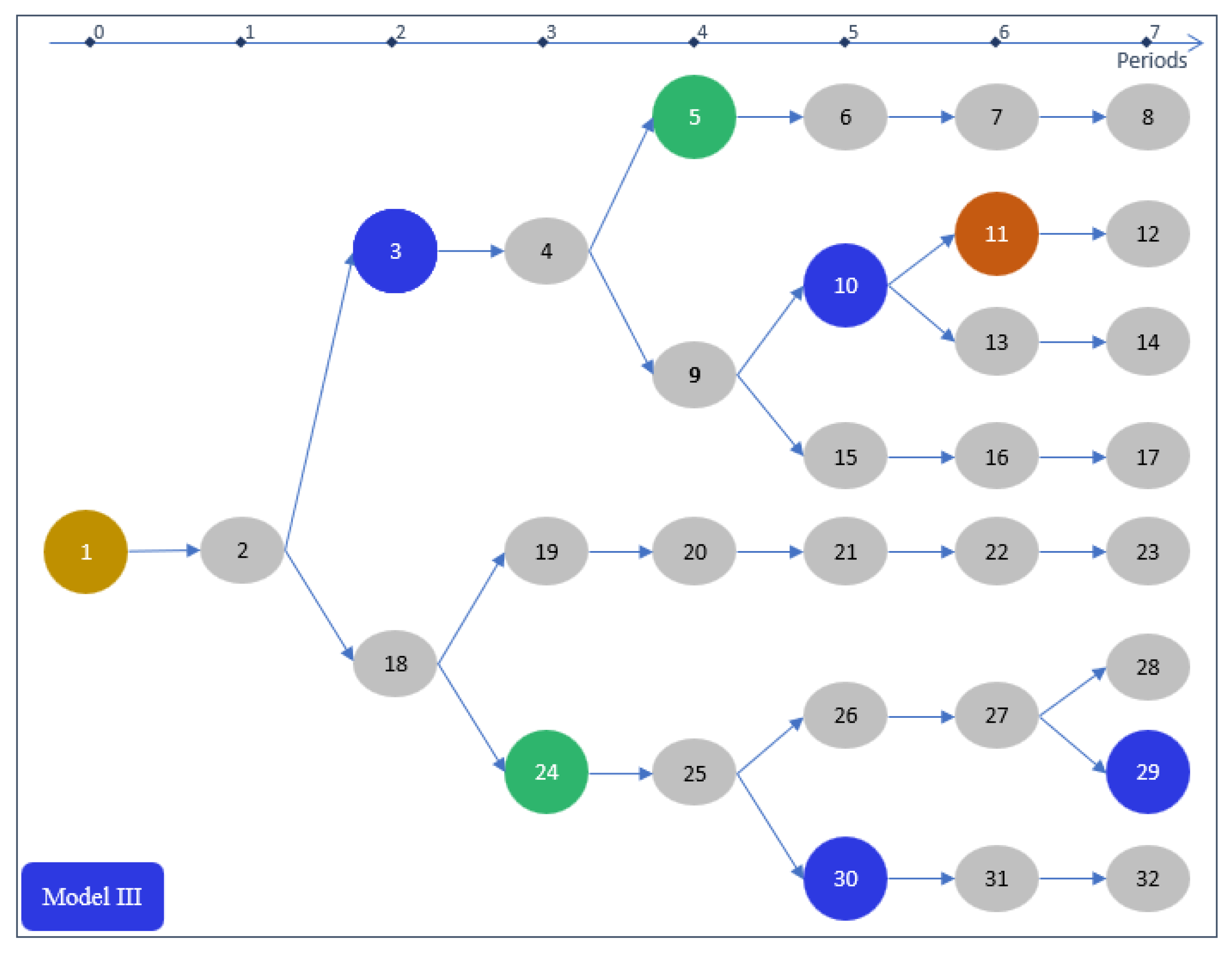
Figure 2.
Model I representation of the management alternatives for the example management unit shown in Figure 1.
Figure 2.
Model I representation of the management alternatives for the example management unit shown in Figure 1.
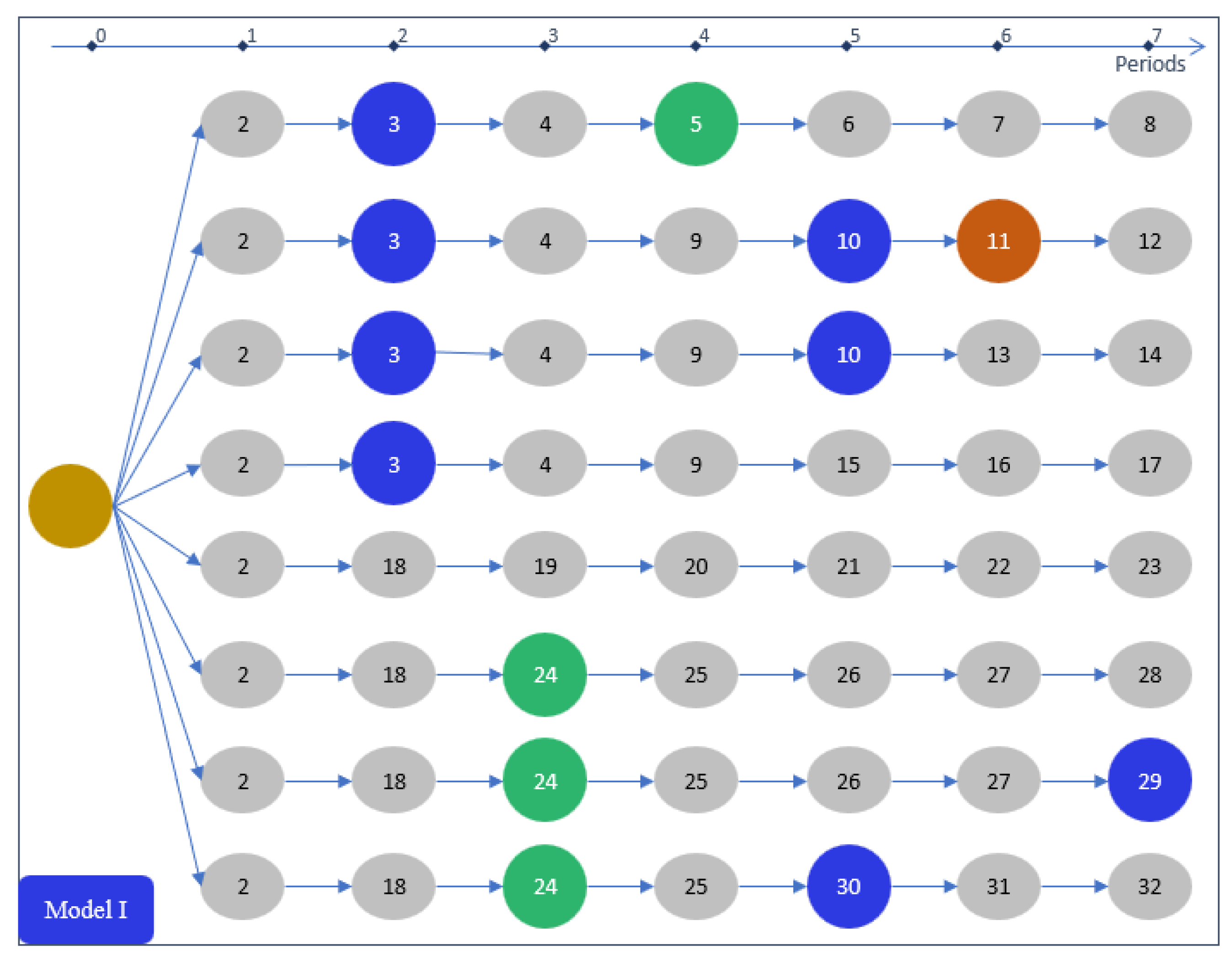
Figure 3.
Model II representation.
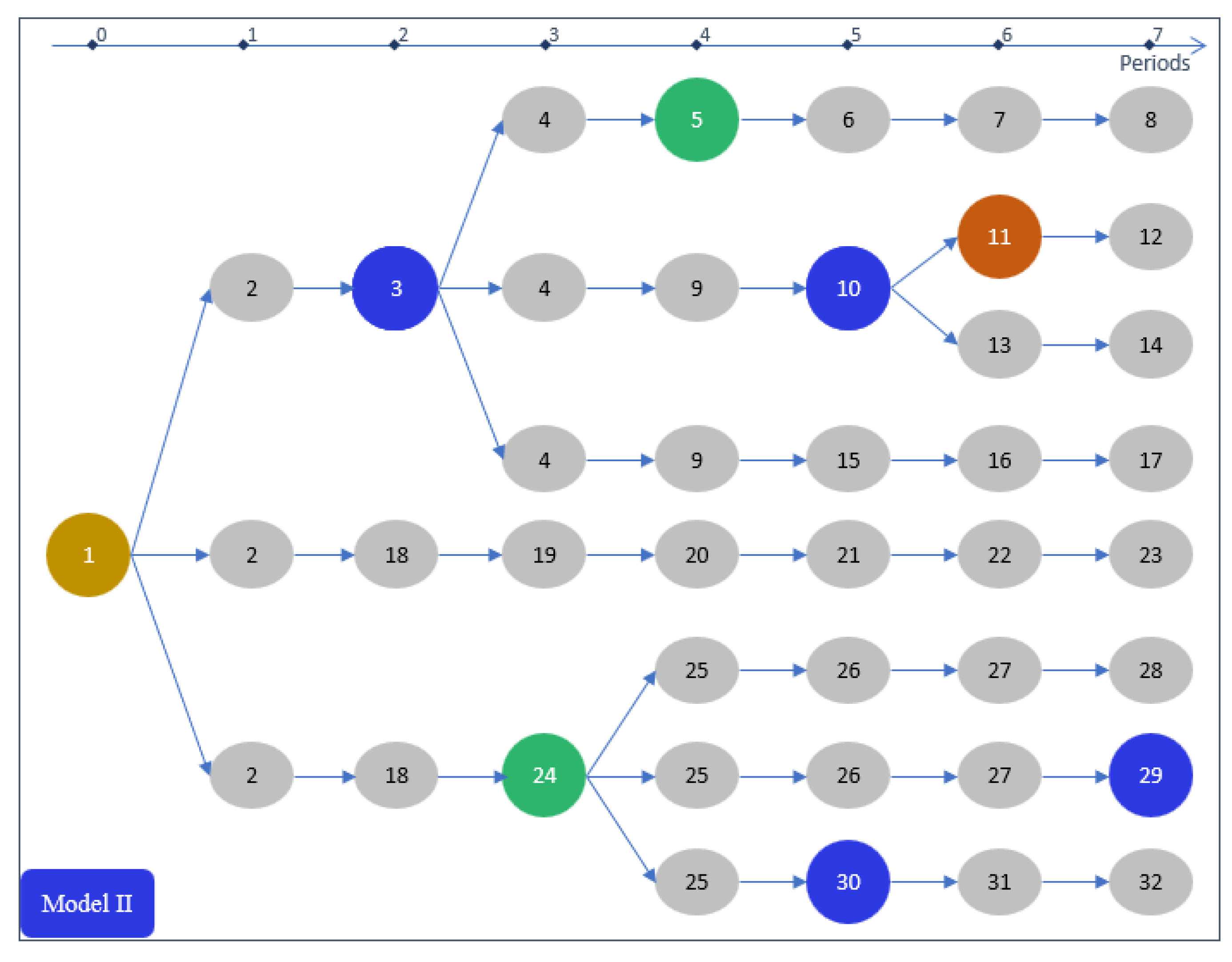
Figure 4.
Building plus solver time.
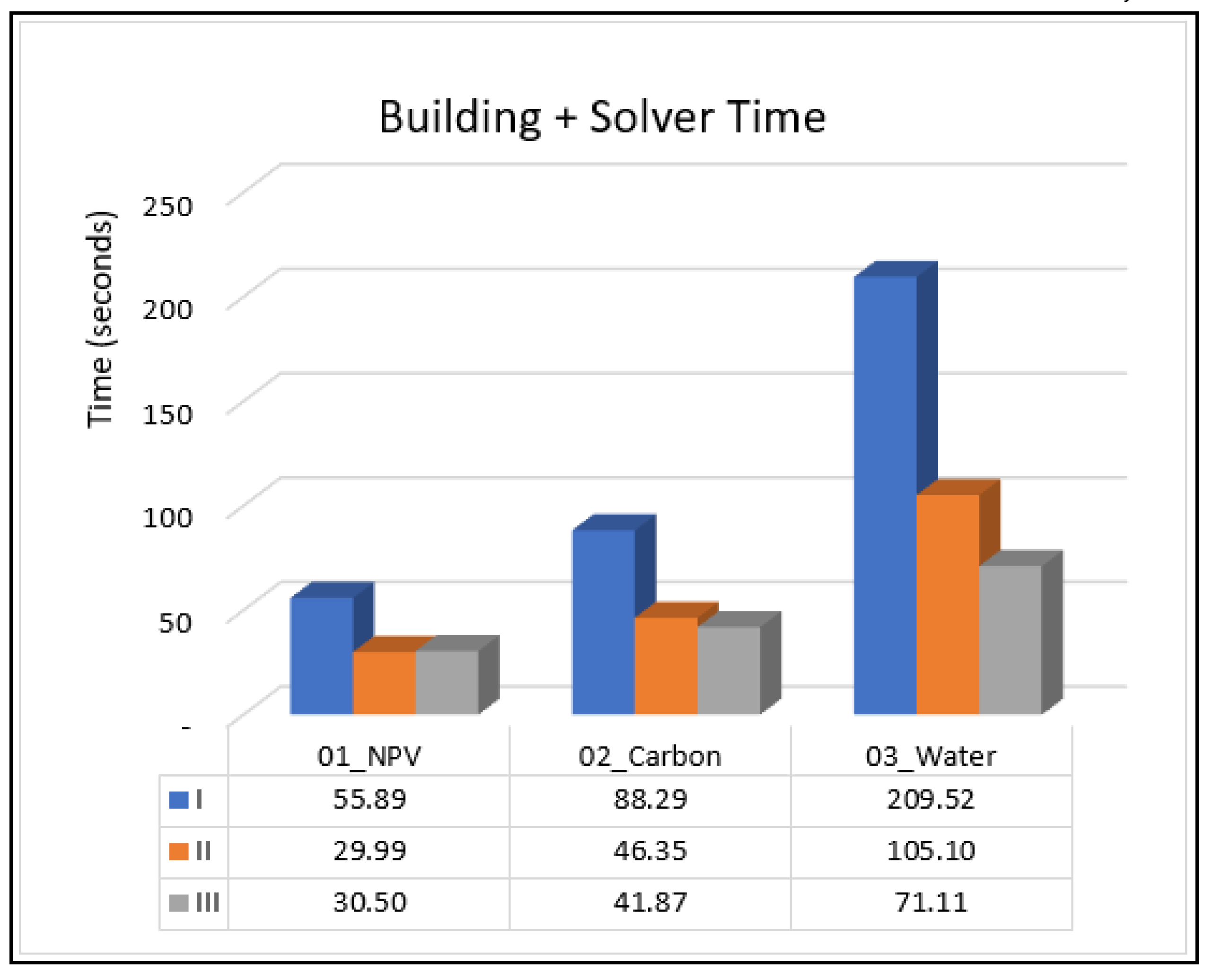
Figure 5.
Accounting constraints building time.

| Models | Set | Nodes and Prescriptions in Figure 1, Figure 2 and Figure 3 |
|---|---|---|
| I, II, III | {0,1,2,3,4,5,6,7} | |
| I, II, III | {1,2,3,4,5,6,7,8,9,10,11, …,29,30,31,32} | |
| I, II, III | 1 | |
| I, II, III | For t=4: {5,9,20,25} | |
| I, II, III | {8,12,14,17,23,28,29,32} | |
| I |
|
{(1,2,3,4,5,6,7,8), (1,2,3,4,9,10,11,12), (1,2,3,4,9,10,13,14), (1,2,3,4,9,15,16,17), (1,2,18,19,20,21,22,23), (1,2,18,24,25,26,27,28), (1,2,18,24,25,26,27,29), (1,2,18,24,25,30,31,32) |
| II | {3,5,10,11,24,30} | |
| II | {2,4,6,7,9,13,15,16,18,19,20,21,22,18,25,26,27,31} | |
| II | {(1,2,3), (1,2,18,19,20,21,22,23), (1,2,18,24)} | |
| II | {(3,4,5), (3,4,9,10), (3,4,9,15,16,17), (24,25,26,27,28), (24,25,26,27,29), (24,25,30), (10,11), (30,31,32), (5,6,7,8), (11,12), (10,13,14)} | |
| III | {2,3,4,5,6,7,9,10,11,13,15,16,18,19,20,21,22,24,25,26,27,30,31} | |
| III | {(1,2)} | |
| III | {(2,3), (2,18), (3,4), (18,19), (18,24), (4,5), (4,9), (19,20), (24,25), (5,6), (9,10), (9,15), (20,21), (25,26), (25,30), (6,7), (10,11), (10,13), (15,16), (21,22), (26,27), (30,31), (7,8), (11,12), (13,14), (16,17), (22,23), (27,28), (27,29), (31,32)} | |
| III | For t=4 {(4,5), (4,9), (19,20), (24,25)} |
The key sets from the three models with the nodes belonging to each set from the example prescriptions in Figure 1.
Table 2.
Costs per Region.
| Region 1 | Region 2 | ||||
|---|---|---|---|---|---|
| Rotation | Rotation | ||||
| Age | 1 | 2 | Age | 1 | 2 |
| 0 | 9,344 | 4,153 | 0 | 9,985 | 4,438 |
| 1 | 788 | 1,053 | 1 | 672 | 663 |
| 2+ | 492 | 658 | 2+ | 420 | 414 |
| Costs in R$/ha.year, 2+=from 2 years old on, rotation 1 are the years after establishment, Rotation 2 are the years after sprouting from stumps. | |||||
Table 3.
Land Expectation Value (LEV).
| Region 1 | Region 2 | |||
|---|---|---|---|---|
| Site Index | Coppice Cycle | LEV | Coppice Cycle | LEV |
| 23 | 7 x 7 | 6,878.63 | 7 x 7 | 7,647.58 |
| 26 | 6 x 6 | 13,114.42 | 6 x 6 | 13,723.09 |
| 29 | 6 x 6 | 21,459.54 | 6 x 6 | 22,068.22 |
| LEV in R$/ha. First number of the coppice cycle means the number of years of the Rotation 1 and second number means the number of years of the Rotation 2. | ||||
Table 4.
Elapsed time summary and objective function values for three model formulations and three scenarios.
Table 4.
Elapsed time summary and objective function values for three model formulations and three scenarios.
| Scenario | Model | Data Retrieval Time (s) | Building Time (s) | Solver Time (s) | Building + Solver Time (s) | Objective Function (thousand BRL) |
|---|---|---|---|---|---|---|
| 01_NPV | I | 9.83 | 47.29 | 8.60 | 55.89 | 294,981 |
| II | 10.40 | 23.45 | 6.54 | 29.99 | 294,981 | |
| III | 10.35 | 18.18 | 12.32 | 30.50 | 294,981 | |
| 02_Carbon | I | 10.59 | 67.65 | 20.64 | 88.29 | 445,695 |
| II | 9.25 | 32.91 | 13.44 | 46.35 | 445,695 | |
| III | 12.25 | 23.94 | 17.93 | 41.87 | 445,695 | |
| 03_Water | I | 11.29 | 182.98 | 26.54 | 209.52 | 437,761 |
| II | 9.87 | 84.75 | 20.35 | 105.10 | 437,761 | |
| III | 10.53 | 49.05 | 22.06 | 71.11 | 437,761 | |
| Elapsed times are measured in seconds. ‘Data Retrieval’ refers to the time to read data and store it in Python dictionary structure. ‘Building’ indicates the time spent preparing the linear programming matrix using Pyomo AML. ‘Solver’ represents the time from sending the model to the solver until receiving the results. | ||||||
Table 5.
Model building time breakdown.
| Building process steps | I | II | III |
|---|---|---|---|
| Look-up tables preparation | 0.01 | 0.01 | 0.03 |
| Sets declaration | 0.24 | 0.39 | 1.06 |
| Parameters declaration | 5.51 | 5.57 | 5.59 |
| Conservation of area declaration | 0.64 | 1.18 | 7.65 |
| Accounting Var VolCut | 14.12 | 6.29 | 3.03 |
| Accounting Var CRemoved | 15.71 | 6.27 | 2.93 |
| Accounting Var DscCosts | 17.66 | 6.23 | 2.96 |
| Accounting Var DscRevenue | 15.24 | 9.50 | 2.94 |
| Accounting Var AgeControl | 16.24 | 8.34 | 4.60 |
| Accounting Var PltCover | 97.60 | 40.95 | 18.28 |
| Constraints | - | - | - |
| Objectives | - | - | - |
| RHS declaration | - | - | - |
| Total | 182.97 | 84.75 | 49.05 |
| Accounting Variable Time % | 97% | 92% | 71% |
| Building time breakdown for Scenario 3, showing the duration of each model building step | |||
Table 6.
Number of decision variables and conservation of area rows for Models I, II, and III.
| Model | |||
|---|---|---|---|
| I | II | III | |
| Decision Variables (Xs) | 84,158 | 147,697 | 426,151 |
| Decision Variables per Management Unit | 240 | 421 | 1,217 |
| Conservation of Area Rows | 350 | 63,889 | 342,343 |
| Decision variables here only include the variables that represent management alternatives for management units. Accounting variables are not included. The second row is the first row divided by 350, which is the number of management units in this problem. Conservation of area rows include Equation Set (2) for Model I, Equation Set (7) and (8) for Model II, and Equations (7) and (10) for Model III. In Model I, the number of conservation area rows coincides with the number of management units. | |||
Table 7.
Number of nonzero coefficients by accounting constraint type and model type.
| Model | |||
|---|---|---|---|
| I | II | III | |
| VolCut | 263,918 | 83,498 | 83,498 |
| CRemoved | 2,186,882 | 903,529 | 418,120 |
| DscCosts | 2,194,603 | 911,250 | 425,841 |
| DscRevenue | 2,188,819 | 905,466 | 420,057 |
| AgeControl | 1,930,685 | 827,752 | 342,343 |
| PltCover | 1,285,305 | 543,212 | 224,799 |
| Number of non-zero coefficients for each accounting constraint set in this study for each model type | |||
Table 8.
Gurobi presolve report.
| Model I | Model II | Model III | |||||
|---|---|---|---|---|---|---|---|
| Scenarios | Before | After | Before | After | Before | After | |
| 01_NPV | |||||||
| Columns | 84,261 | 51,580 | 147,800 | 54,959 | 426,254 | 54,959 | |
| Rows | 803 | 411 | 64,342 | 2,530 | 342,796 | 2,530 | |
| Nonzeros | 2,437,224 | 213,781 | 1,342,663 | 172,361 | 1,423,744 | 172,361 | |
| 02_Carbon | |||||||
| Columns | 84,282 | 76,336 | 147,821 | 88,086 | 426,275 | 90,947 | |
| Rows | 837 | 438 | 64,376 | 12,188 | 342,830 | 15,049 | |
| Nonzeros | 5,617,575 | 1,371,451 | 2,981,836 | 1,050,952 | 2,111,263 | 638,231 | |
| 03_Water | |||||||
| Columns | 84,492 | 76,357 | 148,031 | 98,265 | 426,485 | 98,907 | |
| Rows | 1,256 | 666 | 64,795 | 22,575 | 343,249 | 23,213 | |
| Nonzeros | 8,128,597 | 3,661,587 | 4,335,300 | 2,272,978 | 2,676,189 | 1,241,941 | |
| Presolve report for each model showing before and after values for columns (variables), rows (constraints), and non-zeros. Summarizes the main presolve metrics, illustrating Gurobi’s effectiveness in simplifying and significantly reducing the size of all three models. | |||||||
Disclaimer/Publisher’s Note: The statements, opinions and data contained in all publications are solely those of the individual author(s) and contributor(s) and not of MDPI and/or the editor(s). MDPI and/or the editor(s) disclaim responsibility for any injury to people or property resulting from any ideas, methods, instructions or products referred to in the content. |
© 2024 by the authors. Licensee MDPI, Basel, Switzerland. This article is an open access article distributed under the terms and conditions of the Creative Commons Attribution (CC BY) license (http://creativecommons.org/licenses/by/4.0/).
Copyright: This open access article is published under a Creative Commons CC BY 4.0 license, which permit the free download, distribution, and reuse, provided that the author and preprint are cited in any reuse.


