Political Competition, Resource Availability, and Conflict: A Simulation

Troy Siemers; Atin Basu; James Hentz

doi:10.20944/preprints202409.1504.v1

Submitted:

18 September 2024

Posted:

19 September 2024

You are already at the latest version

Abstract

This paper explores the dynamics of political competition, resource availability, and conflict through a simulation-based approach. Utilizing agent-based models (ABMs) within an evolutionary game theoretical framework, we investigate how individual behaviors and motivations influence collective outcomes in civil conflicts. Our study builds on the theoretical model developed by Basuchoudhary et al. (2023), which integrates factors such as resource availability, state capacity, and political entrepreneurship to explain the evolution of civil conflict. By simulating boundedly rational agents, we demonstrate how changes in resource availability and state capacity can alter the nature of civil conflict, leading to different equilibrium outcomes. The findings highlight the importance of understanding individual motivations and adaptive behaviors in predicting the stability and resolution of conflicts. This research contributes to the growing body of literature on the use of agent-based models in evolutionary game theory and provides valuable insights into the complex interactions that drive civil violence.

Keywords:

evolutionary game theory

;

civil war

;

state capacity

;

resource availability

Subject:

Business, Economics and Management - Economics

Introduction

Studies on insurgencies often explore why conflicts start, escalate, or end ( see among others, DeRouen & Sobek, 2004, Gleditsch, Saleyhan, & Schultz, 2018, and Findley & Rudoff, 2012). Institutional weakness is frequently cited as a cause, with repressive states being prone to civil war (Young, 2013). However, the type of democratic institutions in ethnically diverse societies also factors into civil war risk; power-sharing institutions reduce risk while majoritarian systems and presidential regimes increase it (Schneider & Wiesehomeier, 2008). Resource-rich states with weak institutions are likely to experience civil war, while those with strong state capacity are less susceptible (Soysa & Neumayer, 2007). Personalist and neo-patrimonial regimes within otherwise weak states are especially vulnerable due to centralized power lacking institutional checks (Gurses & Mason, 2010). Strong political and legal institutions help prevent civil wars by constraining elites and reducing the need for militias. This suggests that civil wars involve struggles for political control and reform (Walter, 2015). Key questions arise about how institutions, resources, and state capacity influence political competition, how violence alters political behavior, and how culture affects these processes. We propose agent-based modeling techniques within an evolutionary game theoretical framework to address these questions.

Agent-based models, or ABMs, are highly beneficial when the link between individual behaviors and collective outcomes is poorly understood or when real-world data collection is impractical or risky. This is especially pertinent when examining civil conflict. Considering individual motivations within a group is crucial when analyzing group dynamics. For example, when studying a rebel group, one must consider the individual motivations that may influence group behavior. Modeling these motivations is challenging, as people rationalize decisions in various ways, even when responding to surveys. ABMs can approximate these behavioral explanations and determine analytical outcomes that are computationally difficult. In summary, ABMs offer a simple yet powerful framework for explaining the dynamics of civil violence, making it easier to comprehend and simulate different social conflicts. Additionally, a computer-assisted approach can simplify complex scenarios, for instance, by reducing an ABM to a stochastic model with two coarse-grained degrees of freedom, capturing the dynamics of civil violence while significantly reducing computation time.

Studies on insurgencies often focus on the reasons behind the start, escalation, or cessation of conflicts (DeRouen & Sobek, 2004; Findley and Rudoff, 2012; Gleditsch et al., 2018). There are competing explanations for rebel motivation, such as the well-known greed versus grievance debate (Collier & Hoeffler, 2004). Conversely, other explanations revolve around resource availability, the opportunity costs of civil conflict, state capacity, and political entrepreneurship. Basuchoudhary, Hentz, and Rhamey (2023) combine all these factors to model a dynamic theory where changes in resource availability can alter the nature of civil conflict. However, the intricate interactions between these factors make empirical confirmation challenging. What's more, even an analytical solution becomes complicated.

This paper uses boundedly rational agents to simulate the evolutionary game theoretic (EGT) framework Basuchoudhary et al. (2023) developed. These agents can evaluate the costs and benefits of their actions and learn how to make better choices. Agent-based methods are precious in evolutionary game theory for modeling complex interactions that are challenging to capture with purely mathematical approaches. These methods allow each agent to be individually modeled, with their own strategies and evolving. This approach is advantageous for studying finite populations, non-vanishing mutation rates, stochastic decisions, and spatial interactions. For example, agent-based simulations can predict evolutionary outcomes in scenarios where traditional mathematical models fall short, such as the weak selection-strong mutation limit (Adami, Schossau, & Hintze, 2014). Therefore, we contribute to a small but growing body of literature using agent-based models by modeling boundedly rational rebel and state actors to demonstrate how the outcome of a civil conflict can evolve toward different results depending on the availability of resources.

This paper in particular follows up on a theoretical paper (Basuchoudhary et al., 2023) that attempts to model the evolution of conflict in the

Basuchoudhary et al. (2023) – Describing the Theory.

Basuchoudhary et al. (2023) model rebels with two possible objectives: Warlord rebels appropriate rents directly, while Reform rebels are motivated by grievances that can be assuaged by capturing state machinery. Rebels of either kind redistribute rents to overcome collective action problems. The drive to capture or challenge the state's authority to control rents helps unite rebels. Rebel leaders may redistribute state resources to their in-group if they gain political power. The state has two possible responses to insurgency: aggressive defense of rent monopoly or making a deal to share rents in the disputed region, depending on the proportion of state elites that cleave to a particular response.

Reform insurgents seek to address the unequal allocation of resources by striving to gain political power. In many African countries, this entails challenging the neo-patrimonial regime and the patron-client networks controlled by the political elite. This often requires a conventional war and a more centralized command to capture a state (Bakke et al. 2012, 270). Furthermore, scholars have explored the inherent coordination challenges in such rebellions. Basuchoudhary et al. (2023) state that rebel leaders can only redistribute resources to their clients if they successfully attain political power.

The Formal Model

Basuchoudhary et al. (2023) model a neo-patrimonial setting where rebels and state elites battle over the distribution of rents. In Nigeria's fiscal federalism system, controlling resource rents or profits in the South differs from the North due to the presence of directly appropriable resources such as oil. Rebels in the South can either steal resources to control rents or demand a greater share. In contrast, insurgents in the resource-poor North can only increase rents by replacing elites through violence or negotiation. The model captures various causes of civil conflict and motivations for controlling rents.

The model is based on the assumption of an ongoing regional conflict between state elites and rebel groups. The rebels are categorized into two types: Warlord (W) with a probability of x, and Reform (R) with a probability of 1-x. In the population, this means that a proportion x of the rebel population is of the Warlord type. This structure emphasizes two conflicting causal theories of rebel behavior – one where the population rebels to secure a direct share of the profits and another where rebels aim to gain control of the state to capture those profits. There are two types of state elite populations: Aggressive (A) with probability y, and Conciliatory (C) with probability 1-y. Aggressive elites are more likely to continue to fight rebellion, while conciliatory elites are more likely to bargain with rebels even when either type of elite begins by fighting rebels.

In this model, individuals adapt their behavior to maximize personal benefits. These adaptive behaviors affect stability outcomes and the possibility of achieving stability, particularly in response to contextual changes. Thus, Warlord rebels can learn to become Reformists or vice versa, just as state elites can learn to become Aggressive even if they start as being Conciliatory or vice versa. This contextual "learning" changes the nature of conflict in the model and is a standard feature of evolutionary game-theoretic modeling. The disputed region generates rents V in any period. Neo-patrimonial leaders exclusively seek rents for redistribution; thus, the state elites and rebels focus on acquiring V.1

Warlord rebels are only interested in obtaining a share of the rents αV where α∈(0,1), without necessarily needing to control the state. They may resort to theft, such as stealing oil directly from underwater pumps, to achieve this. They may also be open to a peaceful arrangement where they can still retain a share of the profits without having to engage in conflict, although they are not opposed to war if it means securing their share of the profits.In regions without directly appropriable resources, capturing the state machinery may be the only way to gain rents. Reformist rebels aim to capture the state in order to obtain and distribute rents in a neo-patrimonial world.

Capturing state machinery can be costly. In a neo-patrimonial system, the state redistributes a fraction of rents V, using 1 - L to run itself and provide public goods. For instance, redistributing rents in Nigeria through the federal structure may incur losses, with L representing "leakage" towards neo-patrimonial redistribution. Essentially, neopatrimonialism involves the state redistributing rents under a "big man." Thus, controlling the state offers a net benefit LV. We assume L is a constant share of rents for simplicity. If warlords capture V, they face lower organizational costs, as they don’t need to maintain ministries or public goods, normalizing their administration costs to zero.

State elites control the state machinery and stand to lose it if defeated by rebels or if they negotiate peace. For insurgents, gaining this machinery is a benefit if they win since they did not possess it initially. Hence, it's a positive LV in the rebels' function when victorious. Conversely, LV represents a loss for state elites if they are defeated by Reform insurgents or granted autonomy. War costs are denoted as C_r for rebels and C_g for state elites, with probability p indicating the likelihood of state elites winning, affecting their expected gains.

Aggressive state elites engage both kinds of rebels in a win-lose scenario. Conversely, conciliatory state elites negotiate with Warlord rebels and share resources. These conciliatory elites might also relinquish control over state apparatus and the associated benefits in a region. Consequently, this results in four potential strategic interactions between the rebels and the state elites, as depicted in the evolutionary stage game illustrated in Table 1.

The analytical solution to this evolutionary game uses the replicator dynamic to delineate an evolutionary pathway toward an equilibrium outcome.2 Rebels from each behavior (Warlord and Reform) interact with state elites from each behavior/phenotype (Aggressive and Conciliatory). Rebel and state elites' interactions are pairwise. This interaction simulates the learning process for boundedly rational players.

The Simulation

In this paper, we eschew analytical solutions in favor of identifying simulated patterns that connect individual motivations to group-level outcomes. The agents in our program can learn; that is, they follow the rules of the replicator dynamic.

The Rebels are divided into Warlords (W) and Reform (R) types with proportions x and 1-x, resp. and the State Elites group is divided into Aggressive (A) and Conciliatory (C) types with proportions y and 1-y, respectively. In our algorithm, we have the following key parameters: total number of rebels, total number of state elites, number of generations, and number of interactions per generation. In specific runs mentioned here, we used 500 total Rebels and 500 total State Elites.

In the first generation, a pair of one Rebel and one Elite are chosen randomly according to the distributions determined by x and y. These two people interact, and payouts are determined according to the payout matrix. This process of choosing pairs and allotting payouts is repeated a certain number of times, say ten times. The payouts from all ten interactions are added to the population counts of the four groups (W,R,A,C), and then the populations of Rebels and State Elites are rescaled back to 500 each, now with different proportions x and y. For example, in one trial with initial values of x_init=0.25 and y_init=.75 we may have (W,R,A,C)=(125,375,375,125) at the start, and after one generation x=0.288 and y=0.802 so the population levels are (W,R,A,C)=(144,356,401,99).

This process is repeated over a set number of generations. In the pictures that follow, the typical number of generations is 150, with ten interactions per generation unless explicitly stated otherwise. If any of the values W,R,A, or C ever hit zero, that group has “died out,” and we stop the process at that generation. This is quite possible if the payouts are much more favorable to one (more) group. This could also happen even if the payout structures are better for a group, but the interactions swing towards another group due to randomness. That is, this is not deterministic. At each generation, we keep track of the values x and y to produce plots to show the evolution of population types over time.

We completed this experiment multiple times, keeping the values C_g and C_r fixed while varying the values of p, V, alpha, and L to see how the behavior of the system changes. We look at two cases when

α < L

and

α > L .

In each of these scenarios, we change the values of p and V to predict the outcomes as individuals learn from the behavior of others in the population.

Discussion

In this section, we highlight some observed regularities in our simulations. The main results are presented in evolutionary phase diagrams. The phase diagrams are unit boxes since x and y are population proportions of rebel warlords and aggressive state elites, ranging from 0 to 1. We ignore population proportions of less than 0 or bigger than 1 in these diagrams since they are meaningless in any realistic setting. The point x* represents the proportion of Warlord rebels where the average payoff or fitness from being Aggressive state elites equals the average fitness for being Conciliatory. Similarly, y* represents the proportion of Aggressive state elites for which the fitness of the Warlord culture equals that of the Reform culture among rebels. Thus, x* and y* are potentially attractors or could be tipping points for behavioral cascades. Without an analytical solution, we will let our simulations reveal the outcomes of learning given a particular initial population distribution.

Bargaining failure over rents is a well-known cause of conflict.3 Thus, the share of rents obtained via controlling the state L and the share received by direct bargaining between the insurgents and the state, α, play essential roles. If state control allows a larger share of rents than a directly bargained approach, the incentive to control the state would presumably be higher. The role of state power in controlling insurgencies is also well-known (Fearon & Laitin, 2003). The phase diagrams below show how the availability of rents V, the relative share of rents, α and L, and state capacity expressed as the ex-ante likelihood the state will win the war, p, determines the type of rebels and state elites – and therefore the nature of conflict – likely to evolve.

Figure 1 is a representative phase diagram in this scenario (Basuchoudhary, Hentz, & Rhamey, 2023).

We notice that when the population of insurgents has a higher proportion of Warlords than x*, then Conciliation is fitter than Aggression – thereby increasing y. Similarly, when y > y*, then x increases. Our simulations, though, provide a more granular link between individuals learning behaviors in a population and their resource and political context.

Scenario 1. L > α.

Scenario 1: L= 0.5, α = 0.25, C_g =1, C_r =1, x_init=0.25, y_init=0.75, i.e. (L > α). In Scenario 2: L= 0.25, α = 0.5, C_g =1, C_r =1, x_init=0.25, y_init=0.75, i.e. (L < α).

In each case, we vary p where p takes the values p = [0.2 0.4 0.6 0.8] while keeping V fixed, and then again, we vary V where V = [5 10 25 40 60] while keeping p fixed. The phase diagrams are available in Appendix 1.

Controlling state power should be advantageous in this case and advantage Reform insurgency. However, the very fact that the state can control resources has an impact on state power itself. Notice that as V rises, the phase diagrams appear to negate the possibility of an attractor – that is, the system does seem likely to reach an equilibrium. Thus, the availability of rents reduces the likelihood of a bargained outcome characterized as one where the conciliatory state culture is part of a stable attractor. Notice further that the system reaches y = 1 only at the very highest level of p – i.e., the state is powerful enough to ensure a victory over the rebels. Thus, the state is likely to be conciliatory only if it is likely to win. This lends credence to the idea that powerful states are more likely to facilitate a bargained solution. The interesting twist is that the Warlord insurgency is more likely to succeed; notice that when p = 0.8, x appears to creep towards 1. Thus, reform insurgencies are less likely to survive when states are powerful – though Warlord insurgencies can. In short, state power seems to drive more of the explanatory power for which type of insurgency is likely to succeed than the availability of rents.

Scenario 2. L < α.

Scenario 2: L=0.25, alpha=0. 5, C_g=1, C_r=1, x_init=0.25, y_init=0.75 (L<α)

This scenario suggests that bargained outcomes should lead to some stable détente with rebels – perhaps even coopting them into the state. There appears to be an apparent attractor – depending on our proxy of state capacity p. When state capacity is low, then the system seems to be attracted toward x = 1 and y = 0. That is, the system favors Warlord rebels and Conciliatory state elites. However, as p rises and state capacity improves, the system shifts toward x = 1 and y =1. That is, irrespective of the availability of rents, state capacity seems to determine the likely conflict outcome.

Conclusion

Our paper models the evolutionary dynamics of state capacity, resource availability, and conflict through a simulation-based approach. We have shown how individual behaviors and motivations can significantly influence collective outcomes in civil conflicts by utilizing agent-based models within an evolutionary game theoretical framework. Our findings underscore the importance of understanding the adaptive behaviors of both rebels and state elites in predicting the stability and resolution of conflicts. The simulations reveal that state capacity plays a more crucial role than resource availability in determining the nature of insurgencies, with powerful states being more likely to facilitate a bargained solution. Additionally, the study highlights that reform insurgencies are less successful than warlord insurgencies. Last, our paper suggests that how resources are shared does matter – that is, if the state has a higher capacity for distributing rents than the nature of conflict, whether the state is likely to be conciliatory or aggressive, and whether rebels are likely to be of the warlord type or reform, differs. These insights suggest that agent-based models in evolutionary game theory can lead to clear, testable hypotheses and provide valuable perspectives on the complex interactions that drive civil conflict.

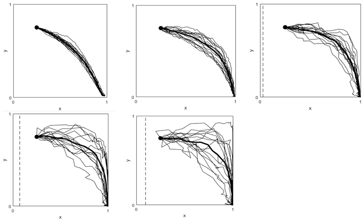
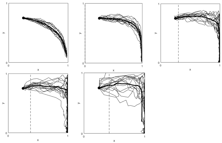
Appendix A. L > α.

15 trials for each case along with the averages: p = [0.2 0.4 0.6 0.8] and V = [5 10 25 40 60]

Case p = 0.2, V ranging [5 10 25 40 60]. Here y* = 0.385 and x* ranging [-0.154,0,0.092,0.115,0.128]

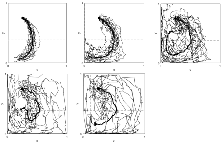
Case p = 0.4, V ranging [5 10 25 40 60]. Here y* = 0.454 and x* ranging [0,0.18,0.29,0.318,0.33]

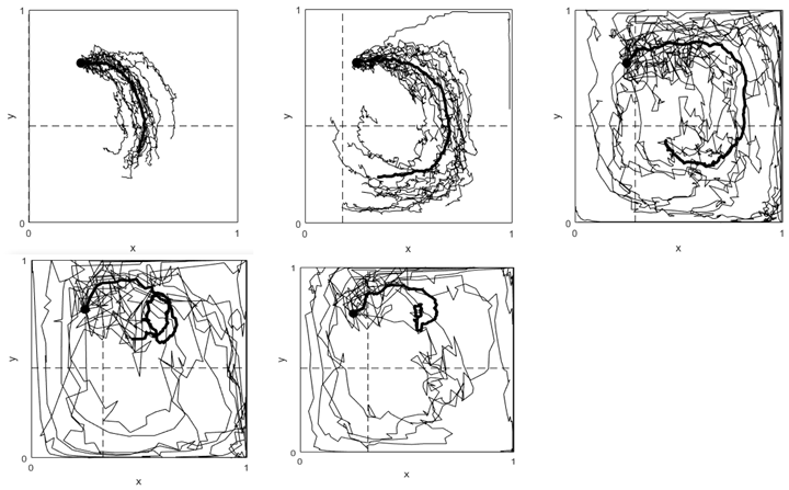
Case p = 0.6, V ranging [5 10 25 40 60]. Here y* = 0.556 and x* ranging [0.22,0.44,0.58,0.61,0.63]

Case p = 0.8, V ranging [5 10 25 40 60]. Here y* = 0.71 and x* ranging [0.57,0.86,1.03,1.07,1.09]

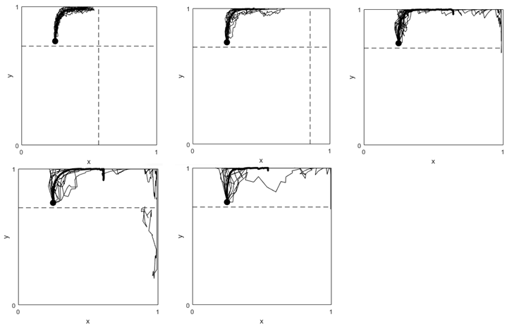
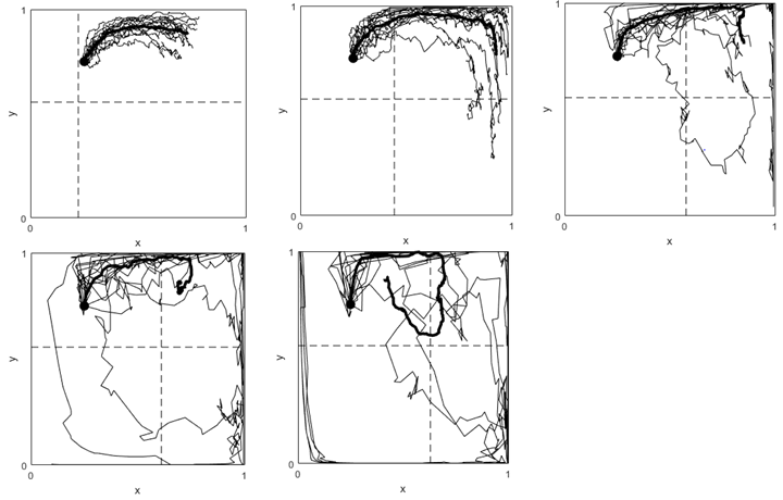
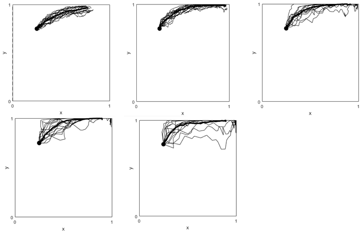
Appendix B. L < α

15 trials for each case along with the averages: p = [0.2 0.4 0.6 0.8] and V = [5 10 25 40 60]

Case p = 0.2, V ranging [5 10 25 40 60]. Here y* = -0.71 and x* ranging [-0.43,-0.14,0.03,0.07,0.09]

Case p = 0.4, V ranging [5 10 25 40 60]. Here y* = -1.25 and x* ranging [-0.2,0,0.3,0.38,0.42]

Case p = 0.6, V ranging [5 10 25 40 60]. Here y* = -5 and x* ranging [-1,1,2.2,2.5,2.67]

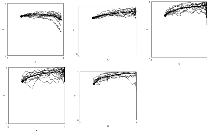
Case p = 0.8, V ranging [5 10 25 40 60]. Here y* = 2.5 and x* ranging [0,-1.2,-1.6,-1.75,-1.83]

References

Adami, C., Schossau, J., & Hintze, A. (2014). Evolutionary game theory using agent-based methods. Physics of life reviews(19), 1-26. [CrossRef]
Bakke, K., Cunningham, K., & Seymour, L. (2012). A Plague of Initials: Fragmentation, Cohesion, and Infighting in Civil Wars. Perspectives omn Politics(10), 265-83. [CrossRef]
Basuchoudhary, A., Bang, J. T., Sen, T., & David, J. (2018). Predicting hotspots: Using machine learning to understand civil conflict. Rowman and Littlefield.
DeRouen, K. R., & Sobek, D. (2004). The Dynamics of Civil Duration and Outcome. Journal of Peace Research, 41(3), 303-20. [CrossRef]
Epstein, J. (2012). Modeling civil violence: an agent-based computational approach. In J. Epstein, Generative Social Science (pp. 247-270). Princeton: Princeton University Press.
Fearon, J. D. (1995). Rationalist Expectations of War. International Organization, 49(3), 379-414. [CrossRef]
Fearon, J. D., & Laitin, D. D. (2003). Ethnicity, insurgency, and civil war. American political science review, 97(1), 75-90. [CrossRef]
Findley, M., & Rudoff, P. (2012). Combating Fragmentationand the Dynamics of Civil Wars. British Journal of Political Science, 42(4), 879-901. [CrossRef]
Gintis, H., & Gintis, H. (2009). The Bounds of Reason: Game Theory and the Unification of the Behavioral Sciences. Princeton: Princeton University Press.
Gleditsch, K. S., Saleyhan, I., & Schultz, K. (2018). Fighting at Home, Fighting Abroad: How Civil Wars Lead to International Disputes. Journal of Conflict Resolution, 52(2), 479-506. [CrossRef]
Gurses, M., & Mason, T. (2010). Weak States, Regime Types and Civil War. Civil Wars, 12, 140-155. [CrossRef]
Haidt, J. (2006). The happiness hypothesis: Finding modern truth in ancient wisdom. Basic Books.
Harrington, J. (2009). Games, Strategies, and Decision Making. New York: Worth.
Hirshleifer, J. (1995). Theorizing about conflict. In K. Hartley, & T. Sandler, Handbook of defense economics, (p. 1650189).
Louie, M., & Carley, K. (2008). Balancing the criticisms: Validating multi-agent models of social systems. Simul. Model. Pract. Theory, 242-256. [CrossRef]
Schneider, G., & Wiesehomeier, N. (2008). Rules that Matter: Political Institutions and the Diversity-Conflict Nexus. Journal of Peace Research, 45, 183-203. [CrossRef]
Soysa, I., & Neumayer, E. (2007). Resource Wealth and the Risk of Civil War Onset: Results from a a New Dataset of Natural REsource Rents, 1970-1999. Conflict Management and Peace Science(24), 201-18. [CrossRef]
Thron, C., & Jackson, E. (2015). Practicality of Agent-Based Modeling of Civil Violence: An Assessment. arXiv preprint arXiv:1501.05838. [CrossRef]
Tullock, G. (n.d.). The Social Dilemma: The Economics of War and Revolution. Blacksburg, VA: University Publications.
Walter, B. (2015). Why Bad Governance Leads to Repeat Civil War. Journal of Conflict Resolution(59), 1242-72. [CrossRef]
Young, J. (2013). Repression, Dissent, and the Onset of Civil War. Political Research Quarterly, 66, 516-32. [CrossRef]
Zou, Y., Fonoberov, V. A., Fonoberova, M., Mezic, I., & Kevrekidis, I. G. (2012). Zou, Y., Fonoberov, V.A., Fonoberova, M., Mezić, I., & Kevrekidis, I.G. (2012). Model reduction for agent-based social simulation: coarse-graining a civil violence model. Physical review. E, Statistical, nonlinear, and soft matter physics, 85(6 Pt 2). [CrossRef]

1	As Tullock (1974) demonstrates, rent-seeking is not just a neopatrimonial vice. To that extent, our model may be generalized to other settings where rent-seeking is a key feature.
2	See Harrington (2009, 507-529) for the simple variant of evolutionary models as used in this paper. Also see Gintis (2009) for a detailed literature review and analysis of how evolutionary modeling may help behavioral scientists understand the evolution of behavior.
3	See, for example, Hirshleifer (1995) and Fearon (1995) for the seminal rationale and Basuchoudhary, Bang, Sen, & David (2018) for an empirical justification.

Figure 1. A representative phase diagram when L> α.

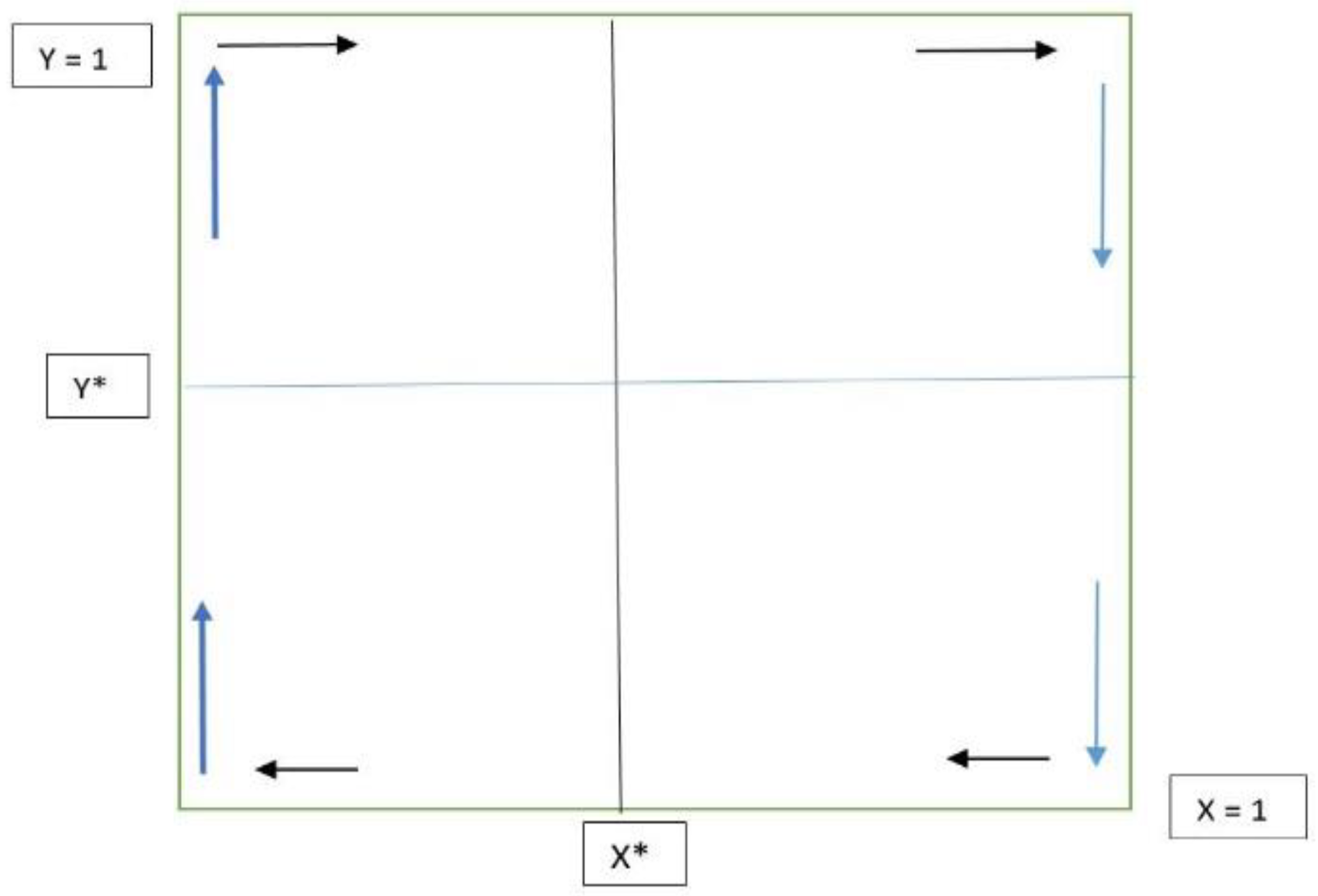
Table 1. The Evolutionary Stage Game.

		State elites
		Aggressive (y)	Conciliatory (1-y)
Rebels	Warlord (x)	$(1 - p) (V - C_{r}) - p C_{r}$ ; $p (V - C_{g}) - (1 - p) C_{g}$	$α V$ ; $(1 - α) V$
Rebels	Reform (1-x)	$(1 - p) (L V - C_{r}) - p C_{r}$ ; $p (- C_{g}) - (1 - p) (C_{g} + L V)$	$L V$ ; $- L V$

Disclaimer/Publisher’s Note: The statements, opinions and data contained in all publications are solely those of the individual author(s) and contributor(s) and not of MDPI and/or the editor(s). MDPI and/or the editor(s) disclaim responsibility for any injury to people or property resulting from any ideas, methods, instructions or products referred to in the content.

© 2024 by the authors. Licensee MDPI, Basel, Switzerland. This article is an open access article distributed under the terms and conditions of the Creative Commons Attribution (CC BY) license (http://creativecommons.org/licenses/by/4.0/).

Copyright: This open access article is published under a Creative Commons CC BY 4.0 license, which permit the free download, distribution, and reuse, provided that the author and preprint are cited in any reuse.