
Submitted:
17 September 2024
Posted:
18 September 2024
You are already at the latest version
Abstract
Real-time simulation of toxic gas dispersion is critical for emergency management in high-sulphur gas fields. The CALPUFF (California Puff model) gas dispersion model, a Lagrangian Gaussian Puff model, is often used in mountainous environments due to its ability to handle complex terrain and weather conditions. Verifying the accuracy of toxic gas dispersion simulations under mountainous conditions is vital for emergency response and rescue. In this article, CALPUFF and Computational Fluid Dynamics (CFD) gas dispersion modeling are compared, studying emissions from a hypothetical pipeline breakout accident in a mountainous area, focusing on range of Semi-Lethal Concentration (LC$_{50}$), Immediate Danger to Life and Health Concentration(IDLH). Thirteen groups of simulation conditions are set up for the experiment, including static wind and winds from the east(E), south(S), west(W), and north(N) at speeds of 1, 2, and 3$m/s$. Comparative experiments between CALPUFF and CFD models show consistent results, confirming the feasibility of CALPUFF for near-field moutainous applications. The overall dispersion range deviation between two methods under calm or light wind of N, E and W is about 300$m$. However,the simulation results of the CALPUFF model and the CFD model show significant differences in S wind. In CALPUFF simulation that the toxic gases are channeled by the valleys, while in the CFD model the toxic gases climb over the mountain top and continue to spread and extend towards the northern valley. The evaluation of CALPUFF’s suitability for applications in near-field mountainous environments indicates its potential use for high-sulfur gas fields and gas dispersion simulations in emergency scenarios.
Keywords:
Mountainous Environment
; High Sulphur Gas
; CALPUFF
; CFD
; Atmospheric Dispersion Model
1. Introduction
China’s high hydrogen sulfide gas reservoirs are mainly located in the Sichuan Basin, producing raw gas with up to 14% hydrogen sulfide content. The areas is also densely populated regions. Risk assessment, leakage monitoring, safety control, and emergency response are vital components for ensuring Quality, Health, Safety, and Environment (QHSE) in high sulfur gas field production. A toxic gas leakage accident will have a significant impact on the surrounding environment and may also cause widespread social impacts[1,2,3]. Therefore, it is an essential task to carry out gas dispersion simulation and establish emergency response and evacuation plans in case of toxic gas leakage accidents.
CALPUFF is a well-established environmental quality regulation guideline supported by the U.S. Environmental Protection Agency (EPA) and is particularly suitable for long-distance pollutant transport (over 50 km)[4,5]. In recent years, the CALPUFF atmospheric dispersion model has been successfully utilized for small-scale gas plant and pipeline scenarios in emergency situations[6]. This model offers faster calculation speeds and enhances calculation accuracy and the capability to handle complex terrain and diverse meteorological conditions[7,8]. However, there are still few studies validating the simulation results of toxic gas pipeline leakage under complex topography conditions. Therefore, we aim to compare the simulation results of CALPUFF and CFD models under complex terrain and meteorological conditions to verify the pattern of toxic gas dispersion simulations and evaluate CALPUFF model for various pipeline leakage emergency scenarios.
Validating atmospheric dispersion simulation is a significant challenge. As for model evaluation, we strive to identify the model that most accurately estimates concentrations in the area of interest. Field experiments are considered the most reliable as they closely replicate real-world conditions. Dedicated gas dispersion field experiments have been conducted, resulting in datasets that can be used for this purpose[9]. For instance, dispersion models have often compared observations from field sampling sites to model simulations[10,11,12,13]. However, the limited number of field experiments cannot provide a comprehensive and reliable evaluation of the models. There are natural fluctuations in the concentration fields due to random turbulence in the atmosphere[14].
Comparative study between wind tunnel experiments and computer simulations is a more feasible method. Atmospheric dispersion models have been validated using wind tunnel experimental data [15,16,17,18]. However, atmospheric dispersion is influenced by many complex factors such as meteorological conditions, topography, land use types, dry or wet deposition, leak source parameters, etc. Different experimental methods and models results lead to different conclusions of environmental assessment, safety risks, and emergency evacuation.
In many studies, two or even more air dispersion simulation models are chosen for comparation and evaluation. For example, studies on the applicability of the AERMOD model and the CALPUFF model mostly focus on specific cases, such as urban areas[19,20], mountainous regions[21,22], industrial parks[23] and so on. Although it is hard to analyze model results from the perspective of data accuracy, comparisons are necessary to analyze the advantages, disadvantages, and applicability of different models. The model performance can be evaluated from different aspects, such as the spatial distribution of gas dispersion, the time taken for pollutants to reach specific locations, concentration peaks, the total concentration during the entire dispersion process, etc. If these different methods can produce similar results, it indicates that these methods can, to some extent, accurately reflect the actual patterns of gas dispersion.
This study examines a hypothetical gas pipeline breakout incident that involves the release and dispersion of high-sulfur gas characterized by complex topography. A qualitative and quantitative comparison is conducted between the CALPUFF model and the CFD model to assess the applicability and reliability of the CALPUFF model within the context of emergency response management systems.
2. Materials and Methods
2.1. Study Area
The study area, shown as the yellow line shaded area in Figure 1, is situated in the mountainous and hilly terrain, characterized by numerous gullies and significant changes in relative elevation. It covers approximately 110 and spans 4 townships, Xiaba, Nanba, Tahe and Gaoqiao. There is a combined resident population of approximately 88,949 until end of 2023. The well sites, pipelines, and valve chambers are close to high-density populated areas, posing significant safety and environmental risks and challenges. In Figure 1, the emergency management zones within 1.5 (yellow line) and 2.5 (purple line) around the pipeline are shown.
The terrain generally ascends from southwest to northeast, marking the transition from the basin hills and low mountains to the middle mountain. The rising and stripping of low mountains and hills dominate the area. The terrain is undulating, with altitudes ranging between 340 m and 1000 m.
The region experiences a subtropical humid monsoon climate, characterized by an average temperature of 16.8 , annual rainfall of 1239.4 mm, and an average wind speed of 1.5 m/s. In spring, summer and autumn, the prevailing wind is from the northeast. In winter, the prevailing wind is from the east. The dominant wind direction is northeast, with a relative humidity of 77%. The area has a long frost-free period, four distinct seasons, and limited sunshine.
Figure 1.
Study Area: Northeast Sichuan, China
As for land use, forest land accounts for the largest portion of the total land area at 37.34%, followed by arable land at 25.55%, and unused land at 22.05%.
This hypothetical leakage accident locates near Qili Village (31.367°N, 108.213°E) in Kaizhou District, Chongqing, shown as Figure 2. The blue circle represents a radius of approximately 500 m from the leakage point. The terrain in this area is very rugged, with many mountains and forests and little flat land. It mainly consists of low mountains and hills with deep valleys and narrow ravines. Roads run along those ravines, and there are dense houses around them. Qili Village is surrounded by various residential areas, including kindergartens, village committees, clinics, primary schools, junior high schools, and nursing homes. These sensitive points are located less than 1,000 m away from the source of the potential leak point, shown as a red circle. In the event of a leakage accident, the consequences could be catastrophic.
2.2. Assumed Scenario
Assuming that the pipeline leakage accident occurs on the hillside between the two valve chambers Q and S, in an extreme scenario, the gathering pipeline undergoes a total break. Due to the pressure drop fast in the pipeline, the Emergency Shutdown Device (ESD) system monitors the leakage signal of the pipeline within 26 s, and the valves can be closed automatically and the separation of the pipeline and other pipelines can be completed in 20 s. Combined with the actual situation and with a certain amount of time remaining, the isolation of the upstream and downstream valve chambers of the pipeline can be completed within 50 s after the total breakage accident occurs. The total leakage volume is the leakage volume before the emergency cut-off valve of the pipeline section, and the residual volume of the pipeline section between the cut-off valves after 50 s of leakage.
Figure 2.
Assumed Leakage Location
According to the above settings, the Phase Model developed by Det Norske Veritas (DNV) is used and the instantaneous emission is used to calculate the leakage rate from the pipeline, and the curve of leakage emission rate is obtained as shown in the Figure 3. In this figure, the risk assessment consideres the most deadly scenario of a full pipeline breakout, and the leakage source emission rate between the two valve chambers Q and S is calculated.
Figure 3.
Leakage Emission Rate Curve
The overall assumed leakage parameters are as follows:
(1)The pipeline length is 5 km, the pipe diameter is 500 mm; the pressure is 7.3 MPa;
(2)The volume percentage of is 82.71%, and that of is 9.73%;
(3)The total estimated leaking volume of is 60,566 kg, and the total leakage time is 185 s.
2.3. Modeling Principles
2.3.1. CALPUFF Model
The CALPUFF model is an environmental quality regulation model that has long been supported by the U.S. Environmental Protection Agency (EPA) [4]. As an important air quality simulation tool, it has played a significant role in environmental protection and atmospheric science research. The CALPUFF model is an improved Lagrangian Gaussian model. It is assumed that the concentration contribution of puff at a receptor point follows a Gaussian Eqs.(1) and (2).
where C is the ground level pollutant concentration at the receptor site (); Q is the mass of the pollutant slug (g); , and is the standard deviation of the Gaussian distribution of the pollutants in the X, Y, and Z directions, respectively (m); is the distance from the centre of the smoke mass to the receptor point in the X direction (m); is the distance from the centre of the smoke mass to the receptor point in the Y direction (m); g is the vertical term of the Gaussian equation (m); is the effective height of the centre of the smoke mass above the ground (m); h is the height of the mixed layer (m). The vertical term g explains the multiple reflections between the mixed layer and the ground. If , g will be simplified as . Smoke masses in the general convective boundary layer satisfy this condition several hours after release.
Equation (1) shows that the CALPUFF model uses a Gaussian approach to treat the interior of the puff. The CALPUFF model describes the diffusion of pollutants as a normal distribution along the y-axis and z-axis directions. The diffusion process is divided into puff clusters over multiple time intervals. For a specific reception point, the total concentration is calculated by summing the averages of all the sampling intervals of the surrounding smoke plumes over the basic time step. The model’s outcomes are comparable to those of a Gaussian model, but instead of a simple straight line, the centre line follows the trajectory curve of the wind, which changes in real-time. Therefore, the model combines the characteristics of the Lagrangian and Gaussian models, making it an improved version of the Gaussian model that uses the Lagrangian method. It is also known as the Lagrangian-Gaussian puff model.
The CALPUFF modelling system consists of four parts: (1) geographic and meteorological pre-processors; (2) the CALMET meteorological module; (3) the CALPUFF dispersion module; and (4) the CALPOST post-processor. The workflow is shown as Figure 4.
Unlike AERMOD or other Gaussin models, the CALMET/CALPUFF modeling system has the ability to model calm hours by simulating stagnant puffs. Stagnant puffs are not dispersed via advection (since the wind speed is zero), but may still undergo turbulence-related dispersion. Furthermore, even if the measured wind speed is zero, CALPUFF accounts for other possible flow components, e.g., puff transport caused by divergence or slope flow. Therefore, the model will calculate concentrations during calm periods.The CALPUFF model reflects the effects of complex terrain by modifying the 3D wind field in the CALMET meteorological module. For some special geomorphological conditions, such as isolated mountains, the model can be set up with secondary terrain to simulate obstacles to the airflow. The algorithm is encapsulated in the Complex Terrain Algorithm for Sub-grid Scale Features (CTSG) module.
2.3.2. CFD Principles
Computational Fluid Dynamics (CFD) is a commonly used method for studying the atmospheric dispersion pattern following hydrogen sulfide leakage from a natural gas pipeline. The primary objective is to elucidate the temporal changes in the density, pressure, velocity, and temperature of hydrogen sulfide gas. The following assumptions are made: after the leakage of a natural gas pipeline, hydrogen sulfide gas is in a state of high pressure and high velocity flow. However, only the exchange and dispersion with the surface air are considered, which is consistent with the standard model of turbulence distribution. Furthermore, the gas flow in the three-dimensional space is considered to be a constant temperature transport.
(1) mass conservation equation
Where: u, v, w are the components of the velocity vector in the x, y, z direction.
(2) turbulent pulsation kinetic energy equation
Turbulent kinetic energy dissipation equation
Where: is the fluid density, ; k is turbulent kinetic energy, ; is the dispersion rate, ; is source term of turbulent kinetic energy equation; is source term of dissipation rate equation; is the hydrogen sulphide-air flow velocity in the direction of grid i, ; and correspond to the i, j directions of the grid, respectively; is the turbulent kinetic energy generated by the velocity gradient; is the dynamic viscosity of the fluid; , , is the corresponding value for turbulent kinetic energy and turbulent dissipation rate, Planck’s number; Finally, , , and are empirical constants.
(3) conservation equation for components
where is the molar concentration of component (); is the diffusive molar concentration of component (); is the diffusion coefficient of the gas ().
The most commonly used software for CFD calculations is that produced by COMSOL, ANSYS Fluent, FLACS, and other similar software. In this study, COMSOL Multiphysics is selected for the simulation and solution processes. The main steps are as follows, shown as the Figure 5:
(1) Constructing the physical model. The topographic map where the accident occurred is used to create a Digital Elevation Model (DEM) with a range of 64 . This data then are imported into Rhino, a three-dimensional modelling software, to generate a three-dimensional surface physical model and a leakage pipeline model. Finally, the model is imported into COMSOL software for Boolean operations to create a 6 km × 6 km × 2.5 km cubic model, which represents the surface above the earth’s surface. This resulted in a vertical space of approximately 300 – 2200 m above the ground surface, which was established as the simulation range for the experiment.
(2) Setting the physical field. The standard turbulence Navier-Stokes model is selected and coupled with the component models. The mixed materials of hydrogen sulphide and air condition are set, as were the properties of the inlet, outlet and wall of the fluid region.
(3) Setting Grid division. The tetrahedral grid is employed as the fundamental division unit, with local encryption of the grid at the mouth of the leakage pipe.
(4) Model Simulating. The simulating is conducted using a pressure, concentration solver multi-field coupling for transient solution.
(5) Export and post-processing of simulation results. The calculation results can be displayed in a variety of formats, including contour, gradient, vector, particle flow traces, three-dimensional slicing, transparent and semi-transparent, and other graphical methods through the post-processing module.
2.4. Qualitative and Quantitative Comparative Analysis
2.4.1. Ranges of the LC50 and IDLH
Hydrogen sulphide is a potent neurotoxicant that can cause irritation to skin and mucous membranes. It is also an explosive gas, with an explosion limit range of 4.0% to 46% (volume ratio). The natural gas in our research contains 8.28-14.25% hydrogen sulphide. has a significant impact on the human body. Once it reaches lethal concentration, the human body quickly loses consciousness, and without prompt rescue, respiration will cease, leading to death.
In the field of environmental impact assessment, LC50 is defined as the concentration of a substance that causes unconsciousness after short-term exposure (30 min), cessation of breathing without prompt treatment, dizziness, loss of consciousness and balance, and the need for immediate artificial respiration and/or CPR techniques. IDLH (Immediately Dangerous to Life or Health) concentration is defined as follows: if a worker does not wearing a mask or lacks experience in escaping, and the gas concentration in the work environment reaches a dangerous level, a 30-minute exposure will cause permanent damage to the human body or reduce the level of human health.
For this research, we assume an emergency response time of 30 min. The LC50 threshold of H2S is 986 , which is consistent with toxicity data. However, for consistency with the predicted evaluation results of the Environment Impact Assessment Report, we retain the LC50 threshold of H2S (618 ) and the concentration value of serious injury, IDLH (432 ) with an exposure time of 30 min.
To evaluate the consistency of concentrations obtained from the CALPUFF model and CFD, we compare the contours of surface layer concentration results output from both two models. The ranges of gas dispersion for different hazardous levels is compared, specifically the maximum ranges of the LC50 and the IDLH.
2.4.2. Statistical Performance Measures:FB, NMSE, R, MAE, PBIAS
To evaluate gas concentration obtained from CALPUFF model simulation and CFD experiments, we use the quantitative indexes proposed by Hanna and Chang [14]. Additionally, a resampling method for predicted data is proposed, and the predicted concentration values at discrete points are quantitatively analyzed. We select Fractional Bias (FB) and Normalised Mean Square Error (NMSE) as indicators.
Where P and O represent the CALPUFF model simulation and CFD experiment, respectively. They denote the mean values of the respective sampling points and . The FB and NMSE indicators reflect the overall systematic bias of the data. In the ideal case, when the model and the experimental results are in perfect accordance with each other, the values of FB and NMSE are equal to 0.
Additionally, a correlation coefficient R is selected to reflect the correlation between the two groups of data. When is closer to 1, it indicates a stronger linear correlation between the two sets of data. Conversely, when is closer to 0, it indicates a weaker linear correlation.
Where and are the standard deviations of the sample points for the CALPUFF and CFD simulations, respectively.
MAE and PBIAS also are selected as indicators for quantitative analysis. Mean Absolute Error(MAE) represents the average absolute error between the values predicted by CALPUFF and CFD. It measures the mean of the absolute differences between the two sets of values. Percent Bias(PBIAS) reflects the cumulative deviation between CALPUFF and CFD models. When the models align well, PBIAS provides a more accurate assessment of the overall model performance. An optimal PBIAS value of 0 indicates that the model is in good overall agreement.
3. Results
3.1. CALPUFF Simulation
Table 1 shows the detailed parameters for the dispersion simulation of CALPUFF, including pollution sources, meteorological conditions, and simulation settings. MM5 DOMAIN2 was selected for the upper-air meteorological data, and the horizontal grid spacing, vertical stratification, and number of grid points of CALPUFF were the same as those of CALMET. The input data used the output results of CALMET. The CALPUFF receptor points had a grid spacing of 100 m, a time step of 1 min, and a simulation dispersion time of 60 min. The simulation area was 10 km × 10 km × 3 km with a grid spacing of 50 m. The terrain file used the SRTM1 dataset with a resolution of 30 m, and the land use file used the GLCC dataset with a resolution of 1 km. Thirteen groups of simulation conditions were set up for the experiment, including calm and winds from the E, S, W, and N at speeds of 1, 2, and 3 m/s. Choosing four wind directions instead of eight can significantly reduce the computational load, allowing for more efficient numerical calculations and simulations.

Table 1.
CALPUFF simulation parameters
| Parameter Type | Parameter Name | Value |
|---|---|---|
| UTM coordinates(km) | (234.877 3473.580) | |
| Pollutant | ||
| Pollutant volume concentration | 9.73% | |
| Source attributes | Chimney height (m) | 0 |
| Outlet initial velocity (m/s) | 1 | |
| Emission rate(g/s) | 0.49s:300000 50-184s:190000 after 185s:0 |
|
| Diffusion Type | Point source | |
| Air velocity(m/s) | 0, 1, 2, 3 | |
| Meteorological parameters | Wind direction( ) | 0, 90, 180, 270 |
| Temperature( ) | 7 | |
| Wind field time step (s) | 3600 | |
| Simulation time setting | Concentration field time step (s) | 60 |
| Total duration(h) | 2 | |
| X-direction length(km) | 10 | |
| Simulation range setting | Y-direction length(km) | 10 |
| Grid size(m) | 50 |
3.2. CFD Numerical Simulation
In this experiment, we choose the 6 km × 6 km × 2.5 km area around the pollution source for simulation. In the CALPUFF model, CALMET generates a 3D wind field diagnosis based on the principles of mass conservation and the continuity equation. In CFD simulations, the meteorological parameters, such as wind speed, wind direction, and temperature, are kept consistent with those used in the CALPUFF model. Although CALMET data is not directly utilized in the CFD model, the mass conservation equation and the species transport equation are configured with the same meteorological parameters to simulate the gas flow behavior and the diffusion process of sulfur hexafluoride pollutants.
We focus on the early 30 min of the leakage accident and the high-risk area near the source. The 3D surface physical model and leakage pipeline model were generated with the help of the 3D modelling software Rhino. The Boolean operation was imported into the COMSOL software to cut the 6 km × 6 km × 2.5 km cube to obtain a cubic area for simulation. The area comprises six boundaries: the ground surface, the north-west-south-east air inlet, and the top. The source of the pollutant leakage is situated in the centre of the ground, which is a hexahedron with a length of 10 m, width of 10 m and height of 1 m.
The simulation uses tetrahedral grids as the basic unit of division. The grid scale is encrypted, with an ultra-detailed grid (cell size from 40.6 m to 215 m) used from the ground to the 550 m height, and a regular encrypted grid (cell size from 108 m to 602 m) used from 550 m to 2500 m height. The model is divided into a total of 694 690 domain tetrahedral cells. The experiment has a total simulation time of 60 min, with 6 s time step.
Table 2.
CFD experimental boundary conditions and parameter settings
| Boundary Name | Boundary Type | Parameter Value |
|---|---|---|
| Source vent | Concentration and speed | Concentration was controlled using a segmented function with a leak rate of 1 m/s. The leak concentration was from 0 to 50s, and from 50 to 185s. After 185s, there was no leak. |
| Ground | Zero flux | No slip and no flow boundary, soil material |
| Outer wall of the source | Zero Flux | No slip |
| West inlet | Speed and Pressure | For the velocity boundary, use 0.5, 1, 2, or 3 m/s. For the pressure boundary, use 0 gauge pressure. |
| North inlet | Speed and Pressure | Same as above |
| South inlet | Speed and Pressure | Same as above |
| East inlet | Speed and Pressure | Same as above |
| Top | Pressure | Gauge pressure is 0 |
3.3. Comparative Analysis of LC50 and IDLH Impact Ranges
We measured the maximum distance from the leakage source to the and IDLH boundary under 13 different conditions. The influence ranges of and IDLH measurements, shown as Table 3, are determined using CALPUFF and CFD simulation results.
Table 3.
Comparison of Maximum Impact Distance between Max LC50 and Max IDLH
| Scenario | CALPUFF | COMSOL | Error (CALPUFF-COMSOL) |
|||
|---|---|---|---|---|---|---|
| IDLH(m) | IDLH(m) | (m) | IDIH(m) | |||
| Static | 766 | 847 | 682 | 914 | 84 | -67 |
| North 1 m/s | 1042 | 1121 | 938 | 1196 | 104 | -75 |
| East 1 m/s | 1744 | 2022 | 1861 | 2147 | -117 | -125 |
| South 1 m/s | 2542 | 2698 | 2473 | 2713 | 69 | -15 |
| West 1 m/s | 1052 | 1391 | 1214 | 1365 | 162 | 35 |
| North 2 m/s | 1052 | 1283 | 1132 | 1369 | -80 | -86 |
| East 2 m/s | 1532 | 1756 | 1681 | 1981 | -149 | -225 |
| South 2 m/s | 2002 | 2604 | 2069 | 2338 | -67 | 266 |
| West 2 m/s | 1781 | 1926 | 1801 | 2003 | -20 | -77 |
| North 3 m/s | 821 | 1031 | 855 | 1050 | -34 | -19 |
| East 3 m/s | 1323 | 1572 | 1167 | 1422 | -156 | -150 |
| South 3 m/s | 1919 | 2279 | 1945 | 2242 | 26 | 37 |
| West 3 m/s | 1610 | 1677 | 1582 | 1752 | 28 | -75 |
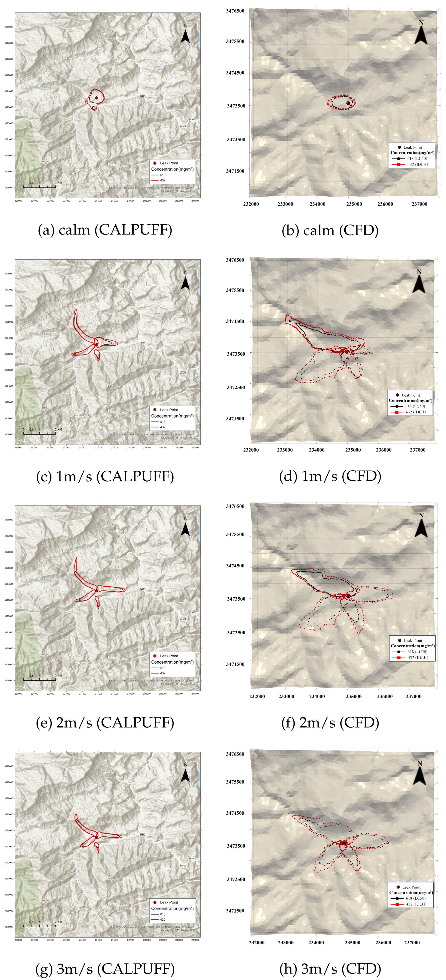
Figure 6 shows concentration predictions from the CALPUFF and CFD models of the 30-min slip-averaged maximum concentration of each grid under 4 wind conditions. This value indicates that the duration of this maximum concentration in each grid is 30 min. The reason for choosing this value is that the time for the semi-lethal concentration of is 30-60 min, and the time for immediate danger to life health (IDLH) time is also 30 min. Black line shows the range of ((618 )) and red line refer to the IDLH ((432 )).
From the topographic map, it can be observed that there are steeper mountains in the north and west of the leakage point than that in south and east, causing toxic gases to diffuse towards the northwest and southwest. It is evident that the steep mountain has a significant impact on the diffusion direction.
Figure 6(a) shows the CALPUFF concentration range of and IDLH under calm wind. It can be seen that the diffusion range of IDLH under calm wind conditions is basically circular with a diameter of about 847 m. Two independent high concentrations of also accumulate in the valley southwest of the leakage source. Figure 6(b) shows the CFD diffusion range of and IDLH under calm wind conditions by using COMSOL. It can be seen that the diffusion range under calm wind conditions is basically an east-west elongated, north-south shortened ellipse, with the maximum IDLH range reaching 914 m, which is similar with CALPUFF results. Under calm wind conditions, the maximum range error for the two models is 84 m.
Figure 6(c) shows the CALPUFF concentration range of and IDLH under wind speeds of 1 m/s in four directions. Figure 6(d) shows the CFD diffusion range under wind speeds of 1 m/s in four direction. It can be observed that the diffusion trends of the two models are similar, both of them are spreading along the valleys and the farthest diffusion direction is S wind. Under S wind direction, the toxic gas extends northwest along the valley with the IDLH range reaching a maximum of 2700 m. The maximum range error for the two models is 125 m.
Figure 6(e) shows the CALPUFF diffusion range of and IDLH under wind speeds of 2 m/s. Figure 6(f) shows the CFD diffusion range under wind speeds of 2 m/s. The trend of two model is similar, with the largest diffusion remaining S wind. Under S wind, the diffusion extends along the northwestern valley, with the IDLH range reaching a maximum of 2600 m. In the N wind, due to the obstruction of the mountains, the diffusion range of IDLH is about 1300 m, which is half that of the S wind. The maximum range error for the two models is 266 m.
Figure 6(g) shows the diffusion range of and IDLH under wind speeds of 3 m/s. Figure 6(h) shows the CFD diffusion range under wind speeds of 3 m/s. Due to the relatively high wind speed, the range of concentration of toxic gas is quickly diluted, reducing the diffusion range about 300 m in 4 directions. The maximum IDLH range under south wind conditions is about 2300 m, extending to the northwest. In the E and W wind, the IDLH ranges also gradually decrease to 165 m and 1670 m respectively. Due to the obstruction of the mountains in the north wind direction, the diffusion range is only 1050 m. The maximum range error for the two models is 156 m.
From Table 3, it can be seen that the results of the CALPUFF and CFD models exhibit high agreement. in the comparison of maximum diffusion range, under calm wind, N, E, S and W, both models show good consistency, with the IDLH range difference about 260 m. As for environmental assessment and emergency management, the maximum range of IDLH and for a leak point using 4-wind-direction or 8-wind-direction calculations is very meaningful.
The two maximum diffusion error 225 m and 266 m of IDLH occurs under S and E wind at 2 m/s.The error is due to the differences in the principles of the two models considering complex terrain. When calculating pollutant diffusion, CALPUFF modifies the three-dimensional wind field model by setting terrain roughness. In contrast, the CFD method generates a three-dimensional finite element grid and uses a terrain roughness function for calculations. During the calculation process, different method causes the slight difference of gas dispersion pattern.
3.4. Quantitative Analysis of CALPUFF and CFD Experiments
Table 4 shows the quantitative evaluation of CALPUFF and CFD experiments under different leakage scenarios. The gas concentrations obtained from the CFD experiments and CALPUFF simulations cannot be compared directly. To achieve quantitative data analysis and comparison, the first step involves converting concentration values, which are the units used by the CALPUFF model, to ensure consistency in data units. Next, we employ Kriging interpolation to resample the data. This process will cover an X-coordinate range of 3 km, a Y-coordinate range of 3 km, with a grid spacing of 0.05 km × 0.05 km, resulting in the creation of two grid files to maintain the spatial consistency of the data. Finally, Eqs. (9), (10), (11),(12),(13) will be used to perform statistical analysis of the FB, NMSE, R, MAE and PBIAS values on the grid points of the resulting data.
Table 4.
Quantitative evaluation of CALPUFF and CFD experiments
| Simulation Scheme | FB | NMSE | R | MAE | PBIAS |
|---|---|---|---|---|---|
| Static | 1.74 | 3.54 | 0.44 | 0.68 | 1364.58 |
| North 1m/s | 0.09 | 0.44 | 0.05 | 0.14 | 9.22 |
| East 1m/s | -0.44 | 0.08 | 0.22 | 0.38 | -35.78 |
| South 1m/s | 1.72 | 25.13 | 0.17 | 3.21 | 1248.93 |
| West 1m/s | 1.89 | 9.67 | 0.57 | 2.03 | 3515.17 |
| North 2m/s | 0.51 | 1.97 | 0.02 | 0.20 | 69.62 |
| East 2m/s | -0.29 | 0.12 | 0.26 | 0.25 | -25.31 |
| South 2m/s | 1.46 | 10.78 | 0.21 | 1.53 | 539.76 |
| West 2m/s | 1.58 | 6.03 | 0.05 | 0.96 | 750.78 |
| North 3m/s | 0.78 | 3.41 | 0.16 | 0.20 | 127.88 |
| East 3m/s | 0.28 | 0.23 | 0.29 | 0.21 | 32.08 |
| South 3m/s | 1.14 | 10.18 | 0.23 | 1.18 | 479.84 |
| West 3m/s | 1.70 | 11.94 | 0.29 | 1.21 | 1167.98 |
The FB and NMSE indices reflect the overall magnitude deviation between the two sets of data, with smaller values indicating a higher degree of fit. Ideally, when the model and experimental results perfectly match, the values of FB and NMSE are both equal to 0. As shown in the table 4, the overall magnitude deviation of FB ranges in E direction, indicating a moderate fit. Other cases show no good fit.
The R index indicates the correlation between the two sets of data, with higher values representing greater correlation. Generally, when 0 < |R| < 0.3, there is a weak positive linear correlation between variables; when 0.3 < |R| < 0.7, there is a moderate positive linear correlation; and when 0.7 < |R| < 1, there is a strong positive linear correlation. As seen in the table 4, all cases show weaker correlations. This might be due to the fundamentally different principles of the two models, resulting in weaker data correlations.
Based on the NMSE, MAE and PBIAS values, the results of CALPUFF and CFD the models for the south and west wind directions are quite large. Although from Table 3, the diffusion direction and maximum diffusion distance are similar, the diffusion patterns are different. Therefore, there is considerable variation under south and west wind conditions. We need a further analysis and improvement in the model’s consistency.
From the quantitative data analysis above, it is clear that the CFD model and the CALPUFF model do not precisely match in terms of data. However, this situation is understandable. Literature review indicates that model comparison studies are primarily conducted between CALPUFF, AERMOD, and other Gaussian models[6] [12], all of which are Gaussian models, leading to smaller data errors and better consistency in metrics such as FB, NMSE, and R. When comparing the CALPUFF model with wind tunnel tests, field measurements, or CFD models, the fundamental principles of these methods are entirely different, and comparisons are generally made using only a subset of sampling points[24]. In this study, we resample and compare models by using a X-Y spatial range, which has made the results difficult to interpret. Reference [25] also shows concentration predictions from the CALPUFF and CFD-LS models of a gas emissions from open-pit is generally disagree in data in all simulations.
3.5. Discussions
The above results and analysis show that the CALPUFF model and CDF model have similar characteristics when simulating gas diffusion cases in mountainous areas:
(1) It can be seen that the results of the CALPUFF and CFD models exhibit high agreement in diffusion direction and maximum diffusion distance.The statistical indicators are not good due to the different principles of wind field calculation. There are differences in the wind field simulation methods between diagnostic modeling (CALMET) and numerical modeling (CFD). The reasons for the poor statistical data are mainly attributed to the complex structure of the flow under terrain condition.
(2) Many researches indicate CALPUFF modeling with calm or very light wind conditions are often associated with high impacts and, for a given application, may result in the overall highest impacts. However, in our experiments, the CALPUFF model results are not significantly greater than the CFD model results in terms of diffusion distance and direction.
(3) According to our research, the evacuation ranges can be designated with 1.5 km at N and W wind direction, 2.0 km for E direction and 2.5 km for S direction. In environmental assessment and emergency management, calculating the worst-case scenario range of IDLH and LC50 for a leak point using 4-wind-direction or 8-wind-direction is meaningful. Regardless of whether it is the CALPUFF or CFD model, the simulation results show that the gases diffuse spread through the valley, where there are numerous human activity hubs such as schools, resident and shops. Therefore, a specific emergency response plan needs to be formulated for this particular scenario. We choose the maximum value from the two calculation results as the reference for the emergency evacuation range.
(4) Compared to the CALPUFF model, which has minute-level computational efficiency, the CFD simulation method has heavier computational demands to produce application results. The CALPUFF model is able to reflect the influence of complex topography on airflow and pollutant distribution. The CALPUFF modeling for complex terrain for emergency scenarios can be used as a dispersion model for high-sulfur gas fields and to perform gas dispersion simulation for emergency situations.
4. Conclusions
Many of China’s high hydrogen sulfide gas reservoirs are located near mountainous and densely populated areas. The research objective is to simulate a hypothetical pipeline breakout in mountainous envionment using two different models and verify the pattern of toxic gas dispersion. The research results can assist QHSE professionals to understand a generalizable dispersion pattern under mountainous region and in developing more effective emergency and evacuation plans and emergency management systems.
In this study, a comparative study between CALPUFF and CFD methods of toxic high-sulfur gas dispersion simulation was carried out. The experimental results show that in the simulation results of the emergency-oriented CALPUFF model, the LC50 and IDLH ranges are basically consistent. The overall dispersion range deviation between the CFD model calculation results and the CALPUFF calculation results is not more than 266 m. Comparison experiments confirm the usability of the CALPUFF model in the emergency response platform. Based on this study, the Emergency Response/Management System (ERMS) for the high-sulfur gas field can be developed. Further analysis would be required to verify the computation of the wind field by the two models and to provide more consistent results for complex topography scenarios.
Author Contributions
Conceptualization, M.L. ; Data acquisition, D.Y. and C.L.; Formal analysis, D.Y. and Z.L.; Funding acquisition, M.L.; Investigation, Y.L.; Methodology, Z.L.; Project administration, M.L.; Resources, M.L. and Y.L.; Software, D.Y. and C.L.; Supervision, M.L.; Validation, D.Y. and Z.L.; Visualization, C.L.; Writing—original draft,M.L., C.L.; Writing—review and editing, M.L.. All authors have read and agreed to the published version of the manuscript.
Funding
This research received no external funding
Institutional Review Board Statement
Not applicable.
Informed Consent Statement
Not applicable.
Data Availability Statement
Not applicable.
Acknowledgments
The authors appreciate the help of Rongqian Zhang who participated in this study.
Conflicts of Interest
The authors declare no conflict of interest.
References
- Jianfeng, L.; Bin, Z.; Yang, W.; Mao, L. The unfolding of ‘12.23’ Kaixian blowout accident in China. Safety Science 2009, 47, 1107–1117. [Google Scholar] [CrossRef]
- Hou, J.; mei Gai, W.; yi Cheng, W.; feng Deng, Y. Hazardous chemical leakage accidents and emergency evacuation response from 2009 to 2018 in China: A review. Safety Science 2021, 135, 105101. [Google Scholar] [CrossRef]
- Pang, L.; Li, W.; Yang, K.; Meng, L.; Wu, J.; Li, J.; Ma, L.; Chen, S.; Liang, Y. Civil gas energy accidents in China from 2012–2021. Journal of Safety Science and Resilience 2023, 4, 348–357. [Google Scholar]
- Scire, J.; Strimaitis, D.; Yamartino, R. A user”s guide for the CALPUFF dispersion model. Earth Tech, Inc 2000, 521. [Google Scholar]
- Irwin, J.S.; Scire, J.S.; Strimaitis, D.G. A Comparison of CALPUFF Modeling Results with CAPTEX Field Data Results. In Air Pollution Modeling and Its Application XI; Springer US: Boston, MA, 1996; pp. 603–611. [Google Scholar] [CrossRef]
- Dresser, A.L.; Huizer, R.D. CALPUFF and AERMOD Model Validation Study in the Near Field: Martins Creek Revisited. Journal of the Air & Waste Management Association 2011, 61, 647–659. [Google Scholar]
- MacIntosh, D.L.; Stewart, J.H.; Myatt, T.A.; Sabato, J.E.; Flowers, G.C.; Brown, K.W.; Hlinka, D.J.; Sullivan, D.A. Use of CALPUFF for exposure assessment in a near-field, complex terrain setting. Atmospheric Environment 2010, 44, 262–270. [Google Scholar] [CrossRef]
- Yang, D.; Li, M.; Liu, H. A Parallel Computing Algorithm for the Emergency-Oriented Atmospheric Dispersion Model CALPUFF. Atmosphere 2022, 13. [Google Scholar] [CrossRef]
- Brown, K.J. Rocky Flats 1990–91 winter validation tracer study: Volume 1 1991. [CrossRef]
- Hodgin, C.R.; Smith, M.L. Model validation protocol for determining the performance of the terrain-responsive atmospheric code against the Rocky Flats Plant Winter Validation Study 1992.
- Irwin, J.S.; Hanna, S.R. Characterising uncertainty in plume dispersion models. 25, 16.
- Rood, A.S. Performance evaluation of AERMOD, CALPUFF, and legacy air dispersion models using the Winter Validation Tracer Study dataset. Atmospheric Environment 2014, 89, 707–720. [Google Scholar]
- Holnicki, P.; Kałuszko, A.; Trapp, W. An urban scale application and validation of the CALPUFF model. Atmospheric Pollution Research 2016, 7, 393–402. [Google Scholar] [CrossRef]
- Chang, J.C.; Hanna, S.R. Air quality model performance evaluation. Meteorology and Atmospheric Physics 2004, 87. [Google Scholar] [CrossRef]
- Dong, X.; Zhuang, S.; Fang, S.; Li, H.; Cao, J. Site-targeted evaluation of SWIFT-RIMPUFF for local-scale air dispersion modeling around Sanmen nuclear power plant based on multi-scenario wind tunnel experiments. Annals of Nuclear Energy 2021, 164, 108593. [Google Scholar] [CrossRef]
- Yassin, M.F.; Alhajeri, N.S.; Elmi, A.A.; Malek, M.J.; Shalash, M. Numerical simulation of gas dispersion from rooftop stacks on buildings in urban environments under changes in atmospheric thermal stability. Environmental Monitoring and Assessment 2021, 193, 22. [Google Scholar] [CrossRef]
- Jiang, X.; Yang, H.; Lin, G.; Dang, W.; Yu, A.; Zhang, J.; Gu, M.; Ge, C. Measurements and predictions of harmful releases of the gathering station over the mountainous terrain. Journal of Loss Prevention in the Process Industries 2021. [Google Scholar]
- Zhang, R.; Li, M.; Ma, H. Comparative study on numerical simulation based on CALPUFF and wind tunnel simulation of hazardous chemical leakage accidents. Frontiers in Environmental Science 2022, 10. [Google Scholar] [CrossRef]
- Mak, J.; Taylor, C.; Fillingham, M.; McEvoy, J. Comparison of the Performance of AERMOD and CALPUFF Dispersion Model Outputs to Monitored Data. Air Pollution Modeling and its Application XXVI; Mensink, C., Gong, W., Hakami, A., Eds.; Springer International Publishing: Cham, 2020; pp. 357–362. [Google Scholar]
- Holnicki, P.; Kałuszko, A.; Trapp, W. An urban scale application and validation of the CALPUFF model. Atmospheric Pollution Research 2016, 7, 393–402. [Google Scholar] [CrossRef]
- Tartakovsky, D.; Broday, D.M.; Stern, E. Evaluation of AERMOD and CALPUFF for predicting ambient concentrations of total suspended particulate matter (TSP) emissions from a quarry in complex terrain. Environmental pollution 2013, 179, 138–45. [Google Scholar]
- Tartakovsky, D.; Stern, E.; Broday, D.M. Comparison of dry deposition estimates of AERMOD and CALPUFF from area sources in flat terrain. Atmospheric Environment 2016, 142, 430–432. [Google Scholar]
- Jittra, N.; Pinthong, N.; Thepanondh, S. Performance Evaluation of AERMOD and CALPUFF Air Dispersion Models in Industrial Complex Area. Air, Soil and Water Research 2015, 8, ASWR–S32781, Publisher: SAGE Publications Ltd STM. [Google Scholar] [CrossRef]
- Radonjic, Z.; Agranat, V.; Telenta, B.; Herbenyk, B.; Chambers, D.; Ritchie, T. Comparison of near-field CFD and CALPUFF modelling results around a backup diesel generating station. Air and Waste Management Association - Guideline on Air Quality Models 2013: The Path Forward 2013, 2, 1080–1111. [Google Scholar]
- Kia, S.; Flesch, T.K.; Freeman, B.S.; Aliabadi, A.A. Calculating gas emissions from open-pit mines using inverse dispersion modelling: A numerical evaluation using CALPUFF and CFD-LS. Journal of Wind Engineering and Industrial Aerodynamics 2022, 226, 105046. [Google Scholar] [CrossRef]
Figure 4.
Workflow of CALPUFF Simulation
Figure 5.
Workflow of CFD Simulation
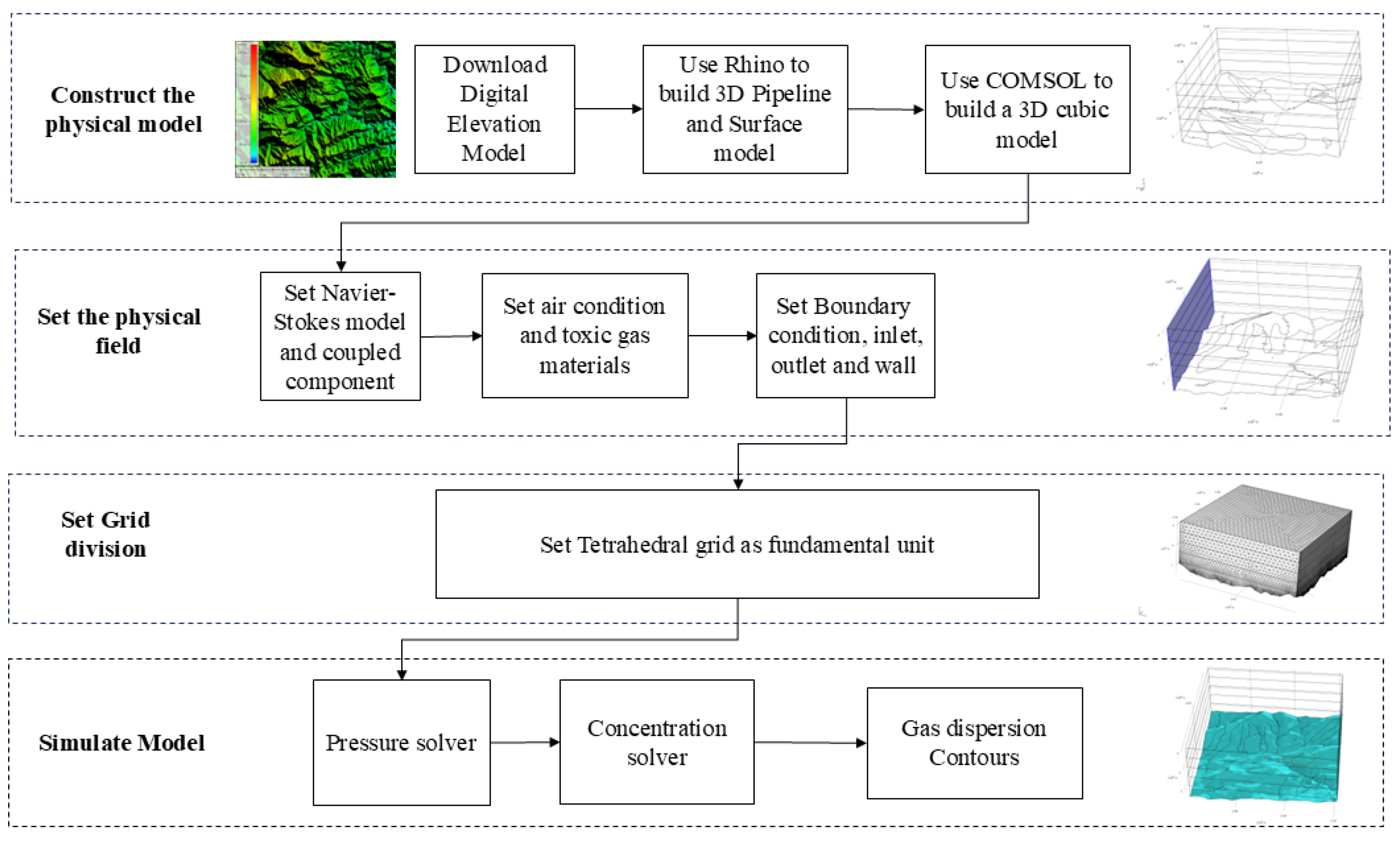
Figure 6.
Slip maximum concentration distributions of CALPUFF and CDF with four directions
Disclaimer/Publisher’s Note: The statements, opinions and data contained in all publications are solely those of the individual author(s) and contributor(s) and not of MDPI and/or the editor(s). MDPI and/or the editor(s) disclaim responsibility for any injury to people or property resulting from any ideas, methods, instructions or products referred to in the content. |
© 2024 by the authors. Licensee MDPI, Basel, Switzerland. This article is an open access article distributed under the terms and conditions of the Creative Commons Attribution (CC BY) license (http://creativecommons.org/licenses/by/4.0/).
Copyright: This open access article is published under a Creative Commons CC BY 4.0 license, which permit the free download, distribution, and reuse, provided that the author and preprint are cited in any reuse.


