Enhancing Cardiovascular Risk Prediction: Development of an Advanced Xgboost Model with Hospital-Level Random Effects

1. Introduction

Ensemble tree based machine learning models including Xgboost have been found to be highly prognostic in cardiovascular medicine.[1] The algorithm’s performance across various clinically significant metrics has been previously assessed using the Clinical Effectiveness Metric (CEM), a consensus-based measure that includes a set of constituent components:[2], [3] Discrimination (AUC[4], F1 score[5]) assesses the model’s ability to distinguish between outcomes, while calibration (1 - ECE[6]) ensures that the predicted probabilities accurately represent the true outcomes. Overall accuracy[7] (1 - Brier score[8]) evaluates the closeness between predictions and actual results, and clinical utility (Net benefit analysis[9]) measures the practical benefit of the model within a clinical setting.

In statistical models, correlation inflates coefficient estimates, resulting in high variability and unstable models.[10] Group levels within the dataset that represent samples from a population or a probability distribution of group levels, i.e. random effects such as cardiac hospitals, could result in the correlation of samples within each group. However, the extent to which ensemble tree machine-learning models can deal with such correlation is largely unknown.

Here, a binary outcome mixed effects Xgboost (BME) algorithm is developed and evaluated using CEM, incorporating hospital as random effects. Scenarios (different sample sizes) under which the model underperforms compared to the fixed effects Xgboost (No cardiac centre: NC) model without random effects is also shown. Commonly used glmer and glm models were also assessed to see how alternative mixed effects machine learning model compare with traditional logistic regression based mixed effects models.

Although mixed effects models incorporating random effects have been widely applied using traditional medical statistics approaches such as in linear mixed and generalised linear mixed models, there are fewer studies (see 1.1 Related work section) on integrating mixed effects into the gradient-boosted tree models for binary classification. Specifically, to the best of our knowledge, the development and application of binary outcome mixed models have been limited to the neural network studies only [11] and [12].

This article is organized as follows: the remainder of Section 1 reviews related work in this area; Section 2 describes the dataset and patient population analysed, the exploratory data analysis undertaken, the proposed Xgboost BME approach and provides the validation approach taken; Section 3 illustrates the application of the method on a cardiovascular dataset; Section 4 gives a discussion in the context of other research as well as some clinical relevance of the approach; Section 5 provides potential future work and limitations of study and finally, a conclusion is provided in Section 6.

1.1. Related Work

Ahlem et al. proposed a mixed-effects random forest (MERF) algorithm developed using Expectation-Maximization (EM) to account for random effects in datasets with continuous dependent variables.[13] In a pilot experimental study, we confirmed that MERF should be used for only continuous outcomes and that for the standard Random Forest there was limited gain in performance when hospital random effects are converted into a high dimensional set of 0 and 1 vectors and considered as fixed effects.[14] Ng et al. applied the EM approach to determine gating network’s weights in a mixture-of-expert based modelling framework for binary mixed effects models.[11] The approach was useful in that the estimated weights can be obtained directly from the log likelihood and enabled faster convergence. However, the approach was based on neural networks. In addition, Giora et al. developed an approach called linear mixed model neural network (LMMNN) that defined a negative log likelihood for binary outcomes using the Gauss Hermite Quadrature approximation to estimate the random effects as part of a mixed effects neural network model.[12]

2. Methods

2.1. Dataset and Patient Population

The study was performed on data from a national cardiac surgery patient registry (Details on the dataset can be found within the Supplementary section: dataset). The registry provides a rich, time-stamped dataset ideal for evaluating the performance of predictive models in clinical settings due to its comprehensive coverage of diverse patient populations and outcomes. It consisted of a total of 227,087 patients over 17 years of age, undergoing cardiac surgery from 42 UK hospitals between 1 Jan 2012 and 31 Mar 2019. The dataset was split into two cohorts: Training/Validation (n = 157,196, 69.2%; 2012-2016) and Holdout (n = 69,891, 30.8%; 2017-2019) as per previous studies[2]. The division into training/validation and holdout cohorts follows standard practices in clinical studies to ensure temporal validation and to assess model generalization to future data.[1] The primary outcome of this study was in-hospital 30 days mortality. As clinical machine learning models with relevance to the tabular dataset is more applicable in the scenario of a large number of variables (i.e., high dimensional) and traditional statistical scores using a small number of variables have already been well studied, this article examined 60 fixed effects variables and 1 random effects variable. The set of 60 fixed effects variables were determined to be clinically relevant upon consultation with two experienced cardiac surgeons. The protocol for this dataset has been described in detail in the experimental pilot study.[14] However, variable selection requires substantial experimentation work, deserving a paper in its own right and hence was excluded from the scope of this study.

2.2. Exploratory Analysis

An exploratory analysis was conducted by visualising variation in the mortality rate (%) across hospitals in the training set and test set using the previously validated approach from [15] for facilitating comparison of patterns across geographical locations (hospitals in this case). Horizontal dashed lines were added at the y-axis value that matched the mean mortality rate across hospitals for the two respective plots.

2.3. Xgboost BME Approach

We define the Xgboost BME as follows:

$$\begin{gathered} y_i= f\left(X_i\right)+Z_i{a}_i \\ {a}_i ~ N(0, {\sigma }_a^2) \end{gathered}$$

(1)

where $f\left(X_i\right)$ represents the complex non-linear function. As in Simchoni et al,[12] $f\left(X\right)=f$ will be used interchangeably from here on; $y_i={[y_{i1}, ... , y_{in}]}^T$ is the $n x 1$ vector of responses for the n observations in cluster i, $X_i={[x_{i1}, \dots , x_{in}] }^T$ is the $n x p$ matrix of fixed effects covariates, $Z_i={[z_{i1}, \dots ,z_{in}]}^T$ is the $n x q$ matrix of random effects covariates, $a_i={[a_{i1}, ... , a_{iq}]}^T$is the i^th random effect cluster of the random effect from the q x 1 unknown vector of random effects having cluster $i={[1,\dots ,m]}^T$.

Unlike Hajjem et al.,[13] the random effects are considered here to encapsulate the variability of the hospitals as well as any sources of unexplained variation that may be associated with difference hospitals. In addition, due to the high computational cost in the context of EM, as well as the rationale that Xgboost uses Boosting rather than Bagging as in Random Forest, the out of bag prediction approach in [13] was excluded from the scope of this study. Since no substantial change was observed in the generalized log-likelihood (GLL) criterion beyond 10 iterations in the pilot experiments and the computational cost of the EM algorithm applied was high, a minimum number of iterations was applied to avoid early stopping. The first iteration was not considered, and the algorithm kept iterating until the absolute change in GLL was less than a given value, such as ${10}^{-10}$.

Step 0. Set r=0. Let $a_{i\left(0\right)}$ = 0, ${\sigma }_{a\left(0\right)}^2$ = 1, $y_{i\left(0\right)}^{*}=y_i$.

Step 1. Set r=r+1. Update $y_{i\left(r\right)}^{*},$ $f_{ij,}$ $a_{i\left(r\right)}$. 

• Build a forest of trees using a standard Xgboost algorithm with $y_{i\left(r\right)}^{*}$ as the training set responses in logit scale and $x_{ij}$ as the corresponding training set of covariates, j=1, …, n. Since logits of $y_{i\left(r\right)}^{*}$ are continuous and binary classification using Xgboost is considered, the values were converted back to binary labels using median as the threshold. Given the high class imbalance, with the outcome class (mortality) constituting fewer than 3% of data, employing the median as a threshold dynamically modifies the decision boundary to better detect rare positive instances. Since the Xgboost now models only the fixed effects component of the response, it was necessary to update the hyperparameters. Random stratified 3-fold Grid Search Cross Validation was applied using the training dataset with the same hyperparameter search criteria as that for the Xgboost NC model similar to previous studies.[1,3] A maximum of 30 combinations was imposed to allow for variability of parameters across iterations.
• Obtain an estimate of $f_{ij(r-1)}$ using the training data on Xgboost in logit scale.
• estimate $a_{i\left(r\right)}$using ${\widehat{y}}_{i(r-1)}$ and $f_{ij(r-1)}$ as inputs into the Gauss Hermite Quadrature using an approach similar to Simchoni et al.,[12] where ${\widehat{y}}_{i(r-1)}=$ ${logit(y}_{i(r-1)}+\epsilon )$. The number of quadrature was set at 80, as determine through pilot experiments, satisfying k < 2m – 1, where k represents the degree of the polynomial for numerical integration and m is the parameter adjusting set here as the number of random effect levels.
• $y_{i\left(r\right)}^{*}$= ${\widehat{y}}_{i(r-1)}$ - $Z_i{a}_{i\left(r\right)}$, i= 1, ..., n, where $y_{i\left(r\right)}^{*}$ represents the fixed component of the response and is re-binarized to 0 and 1 using the median of $y_{i\left(r\right)}^{*}$.

The numerical approximation is utilized to calculate the expected values of the random effects:

E[$a_{i\left(r\right)}$|y] = $\int {\displaystyle \frac{f_{y|a_i}\left(y{|a}_i\right)f_{a_i}\left(a_i\right)}{f_y\left(y\right)}}d{a}_i$= ${\displaystyle \frac{\log \left\{{\sum }_{k=1}^K\exp \left[{\sum }_{j=1}^n\left({\widehat{y}}_{i.}\left({\overline{f}}_{ij}+\sqrt{2}{\sigma }_{a_{\left(r\right)}}^2{x}_k\right)-\log \left(1+e^{\left({\overline{f}}_{ij}+\sqrt{2}{\sigma }_{a_{\left(r\right)}}^2{x}_k\right)}\right)\right)\right]\frac{w_k}{\sqrt{\pi }}\right\} }{{\sum }_{i=1}^m\log \left\{{\sum }_{k=1}^K\exp \left[{\sum }_{j=1}^n\left({\widehat{y}}_{i\left(r\right)}\left({\overline{f}}_{ij}+\sqrt{2}{\sigma }_{a_{\left(r\right)}}^2{x}_k\right)-\log \left(1+e^{\left({\overline{f}}_{ij}+\sqrt{2}{\sigma }_{a_{\left(r\right)}}^2{x}_k\right)}\right)\right)\right]\frac{w_k}{\sqrt{\pi }}\right\}}}$ ,

where:

$f_{a_i}\left(a_i\right)= {\displaystyle \frac{w_k}{\sqrt{\pi }}}$,

$f_y\left(y\right)$ = ${\sum }_{i=1}^m\log \left\{{\sum }_{k=1}^K\exp \left[{\sum }_{j=1}^n\left({\widehat{y}}_{i.}\left({\overline{f}}_{ij}+\sqrt{2}{\sigma }_{a_{\left(r\right)}}^2{x}_k\right)-\log \left(1+e^{\left(f_{ij}+\sqrt{2}{\sigma }_{a_{\left(r\right)}}^2{x}_k\right)}\right)\right)\right]{\displaystyle \frac{w_k}{\sqrt{\pi }}}\right\}$, and ${\overline{f}}_{ij}$ is the mean of estimates from Xgboost on training data. This is also the GLL.

Step 2. Update ${\sigma }_{a_{\left(r\right)}}^2$ using:

Var(E[$y_{ij}$|$a_i$]) = var($f_{i.}$ + $a_i$)

= ${\sigma }_{a_{\left(r\right)}}^2$

= ${\sum }_{i=1}^m{\displaystyle \frac{n_i{\left({\overline{y}}_i-\overline{y}\right)}^2}{m-1}}$

= ${\sum }_{i=1}^m{\displaystyle \frac{n_i{\left({(f}_{i.\left(r\right)}+a_{i\left(r\right)})-\overline{y}\right)}^2}{m-1}}$

where ${\overline{y}}_i=f_{i.\left(r\right)}+ a_{i\left(r\right)}$ is the expectation of the predicted response values at RE level i and $\overline{y}$ is the expectation of the actual response, $y_i$ across all RE levels on the logit scale.

Step 3. Keep iterating by repeating steps 1 and 2 until convergence.

We ran the algorithm 20 iterations and stopped adding additional iterations as there were little change in performance.

The likelihood function is as follows:[12]

$$l = \sum _{i=1}^m\log \left\{\sum _{k=1}^K\exp \left[\sum _{j=1}^n\left(y_{ij}\left(f_{ij}+\sqrt{2}{\sigma }_{a_{\left(r\right)}}^2{x}_k\right)-\log \left(1+e^{\left(f_{ij}+\sqrt{2}{\sigma }_{a_{\left(r\right)}}^2{x}_k\right)}\right)\right)\right]{\displaystyle \frac{w_k}{\sqrt{\pi }}}\right\}$$

(2)

2.4. Validation Approach

2.4.1. Xgboost BME and NC Variant Models

In order to provide a reliable estimate of model performance and its variability, the geometric mean of the Clinical Effectiveness Metric (CEM) and individual component metrics were evaluated using 1000 bootstraps for Xgboost BME and NC model variants that had either features that were standardized or unstandardized. The 95% confidence intervals were also calculated from the bootstrap sampling for the CEM.

Using a similar approach, the CEM and its individual components were assessed for glm and glmer model variants with and without standardization.

2.4.2. Performance by Sample Size

CEM and AUC performances were evaluated against different sample sizes ranging from low (300-1000), medium (2000-10000) to high (15000-full sample size), specifically: 300, 500, 700, 1000, 2000, 5000, 10000, 15000, 15500, 157196. These were evaluated for the two best models from each of the mixed and fixed Xgboost model variants, respectively, i.e.: the unstandardized Xgboost BME and standardized Xgboost NC models. In addition, performance was evaluated for the two best models from each of the mixed glmer and fixed glm model variants, i.e.: standardized glmer and unstandardized glm models. Log₁₀ transform of the sample size was performed along the x-axis of the figures.

2.4.3. Visualization of Parameters

$a_i$ are kept in the log-odds space and plotted across the 42 hospitals by their indices across all the sample sizes in the “Performance by sample size” section. Since $a_i$ contains random effects due to both the hospital and any remaining residual error effects, we centred the $a_i$ effects by subtracting the mean.

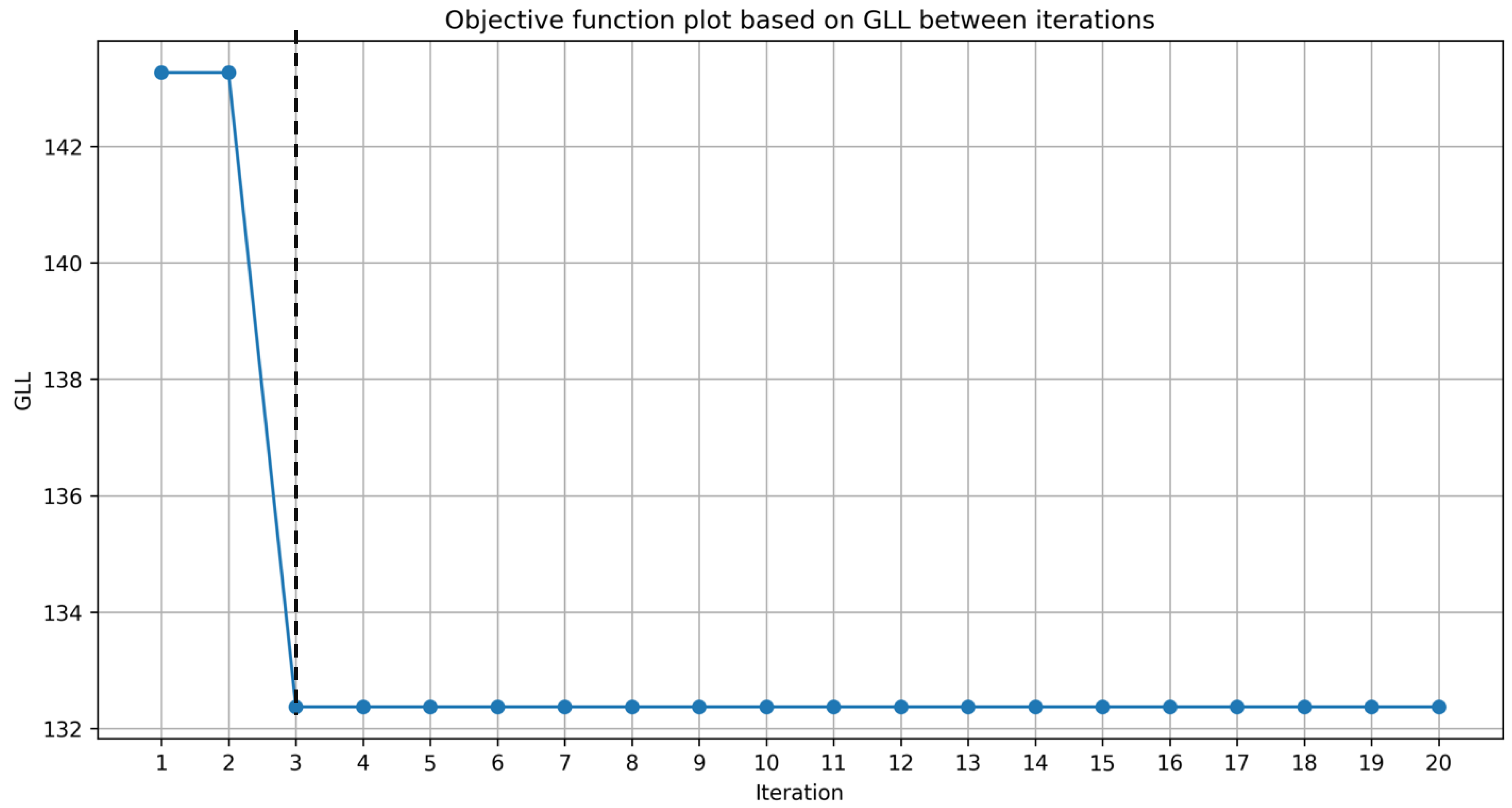
Based on the CEM plot by sample size, the $a_i$ across 20 iterations was visualised for the unstandardized Xgboost BME model at a sample size (n=2000) that showed marked differences between the Xgboost BME and the Xgboost NC models. To show the point of convergence, the GLL objective function is plotted across 20 iterations.

2.4.4. Baseline Models

The study consulted with two cardiac surgeons on the most frequently used logistic regression (LR) models used in their clinical studies. It was found that glm and glmer were the most commonly used and they were not interested in further parameter optimisation for LR in their studies. As such, these models were included as baseline comparison models.

3. Results

3.1. Exploratory Analysis

Figure 1. comparisons of the mortality variation across hospitals in the training and test sets.

Figure 1. comparisons of the mortality variation across hospitals in the training and test sets.

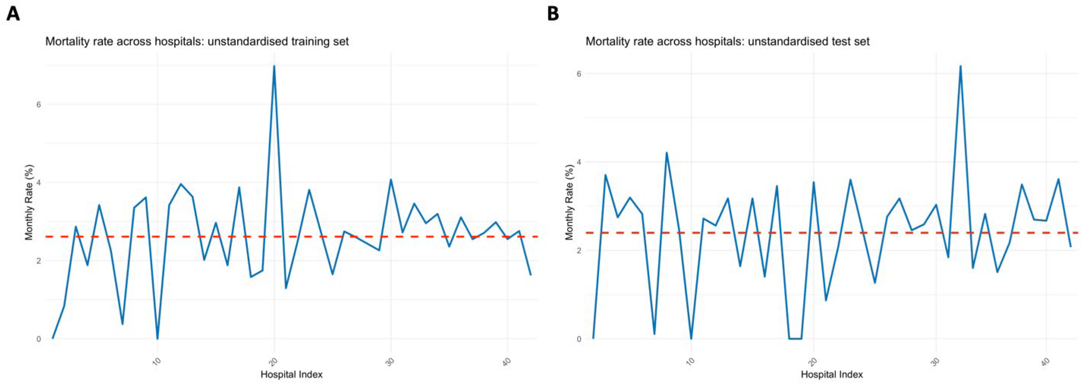
The exploratory analysis showed hospital-related variability in mortality across the training and test datasets. This variability highlights the necessity of accounting for hospital-level effects in predictive modelling, justifying the use of mixed effects models in this context. Notably, the peak near hospital 20 showed a very large peak in the training set, whilst the peaks was diminished in the test set (Error! Reference source not found.). Conversely, the peak at 32 was diminished in the training set but was magnified in the test set.

3.2. Model Validation: Comparison Using All Samples

3.2.1. Xgboost BME and NC Variant Models

The standardized Xgboost NC model demonstrated slightly higher performance (CEM 0.741: 95%CI: 0.7405-0.7411) than other Xgboost model variants when all training data samples were utilised. However, this difference is marginal and may not translate into practical clinical benefits, emphasizing the importance of considering model complexity and interpretability. Unstandardized Xgboost BME and NC performance did not differ (CEM: 0.740) with overlapping confidence intervals. However, the standardised Xgboost BME model showed the lowest performance (CEM: 0.739, 95%CI: 0.7391-0.7397). There were negligible differences across individual component metrics.

Table 1. CEM and individual component metrics for Xgboost BME and NC variant models.

Model Category	ECE	AUC	Brier	F1	Net Benefit	CEM	CEM lower 95% CI	CEM upper 95% CI
standardized Xgboost BME	0.998	0.854	0.977	0.293	0.908	0.739	0.7391	0.7397
unstandardized Xgboost BME	0.997	0.854	0.977	0.294	0.908	0.740	0.7396	0.7402
standardized Xgboost NC	0.997	0.854	0.977	0.295	0.908	0.741	0.7405	0.7411
unstandardized Xgboost NC	0.997	0.854	0.977	0.293	0.908	0.740	0.7394	0.7400

Table 1. CEM and individual component metrics for Xgboost BME and NC variant models.

Model Category	ECE	AUC	Brier	F1	Net Benefit	CEM	CEM lower 95% CI	CEM upper 95% CI
standardized Xgboost BME	0.998	0.854	0.977	0.293	0.908	0.739	0.7391	0.7397
unstandardized Xgboost BME	0.997	0.854	0.977	0.294	0.908	0.740	0.7396	0.7402
standardized Xgboost NC	0.997	0.854	0.977	0.295	0.908	0.741	0.7405	0.7411
unstandardized Xgboost NC	0.997	0.854	0.977	0.293	0.908	0.740	0.7394	0.7400

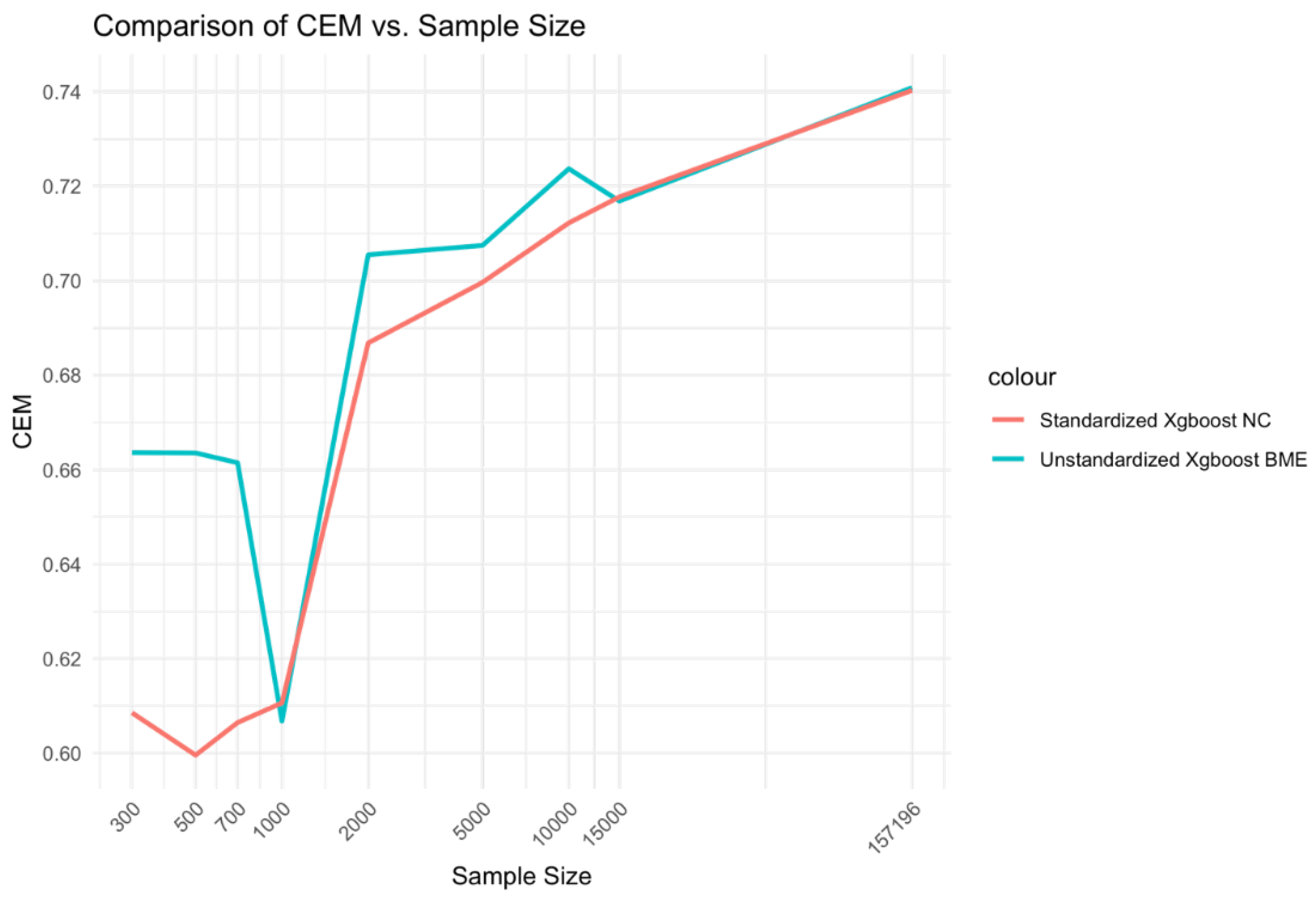
Figure 2. Relationship between sample size and CEM for standardized Xgboost NC and unstandardized Xgboost BME models.

Figure 2. Relationship between sample size and CEM for standardized Xgboost NC and unstandardized Xgboost BME models.

3.2.2. Glmer and Glm Variant Models

The CEM of standardized glmer and unstandardized glm showed a higher magnitude (CEM: 0.719) compared to the other two model variants (CEM: 0.718) due to slightly higher contributions of either AUC or F1 scores, respectively. However, there were very little evidence of the difference being significant across variant models of glmer and glm with confidence intervals overlapping for CEM estimates, ranging from 0.7181-0.7189 (Error! Reference source not found.). AUC values were higher for glmer models (AUC: 0.827) than glm models (AUC: 0.826) suggesting that remaining differences in CEM across models may be mostly attributed to differences in F1 score.

Table 2. CEM and individual component metrics for glmer and glm variant models.

Model Category	ECE	AUC	Brier	F1	Net Benefit	CEM	CEM lower 95% CI	CEM upper 95% CI
standardized glmer	0.993	0.827	0.973	0.269	0.889	0.719	0.7182	0.7188
unstandardized glmer	0.993	0.827	0.973	0.269	0.889	0.718	0.7178	0.7184
unstandardized glm	0.994	0.826	0.973	0.270	0.889	0.719	0.7183	0.7189
standardized glm	0.994	0.826	0.973	0.269	0.889	0.718	0.7181	0.7187

Table 2. CEM and individual component metrics for glmer and glm variant models.

Model Category	ECE	AUC	Brier	F1	Net Benefit	CEM	CEM lower 95% CI	CEM upper 95% CI
standardized glmer	0.993	0.827	0.973	0.269	0.889	0.719	0.7182	0.7188
unstandardized glmer	0.993	0.827	0.973	0.269	0.889	0.718	0.7178	0.7184
unstandardized glm	0.994	0.826	0.973	0.270	0.889	0.719	0.7183	0.7189
standardized glm	0.994	0.826	0.973	0.269	0.889	0.718	0.7181	0.7187

3.3. Performance by Sample Size

3.3.1. Unstandardized Xgboost BME and Standardized Xgboost NC Models

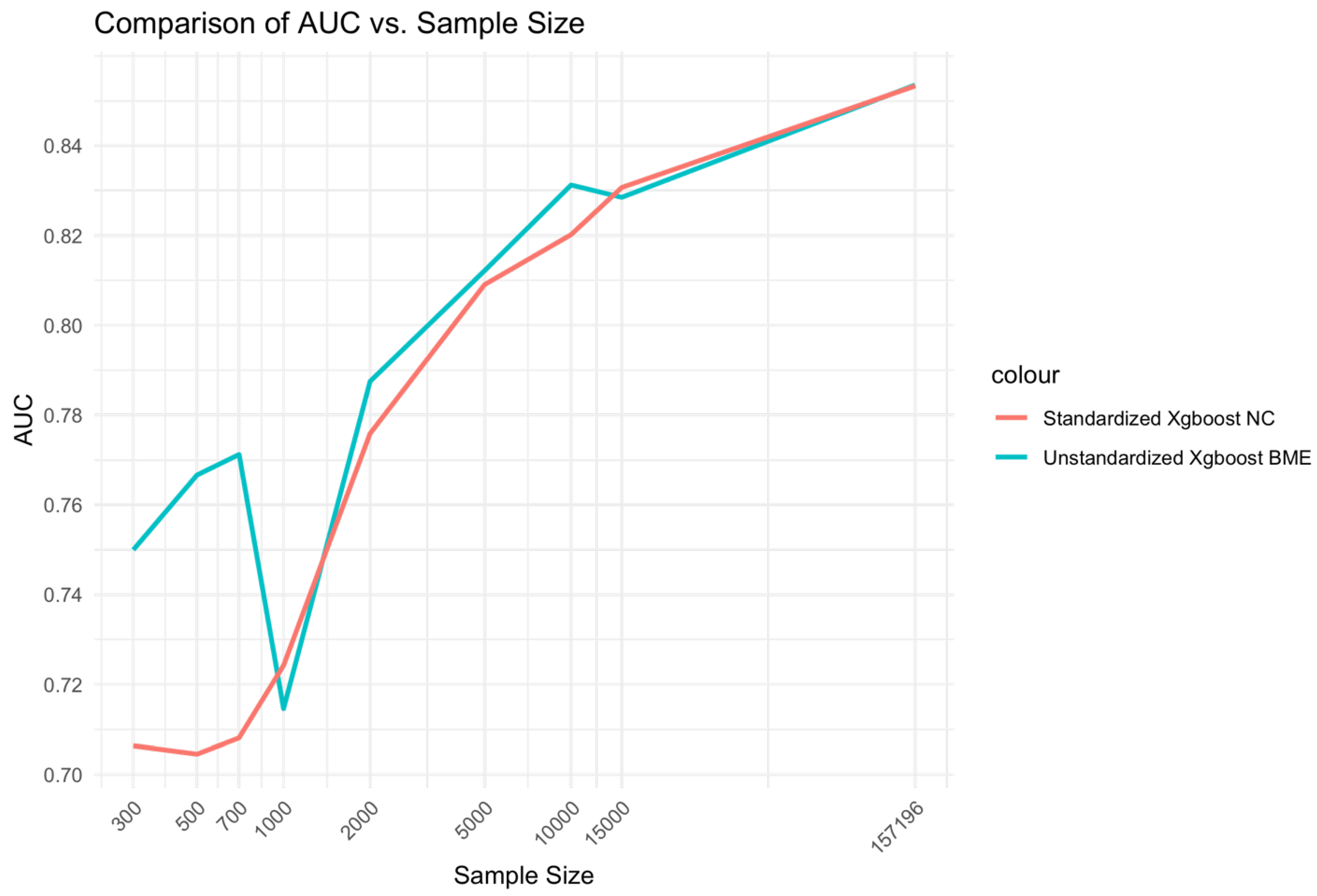
At low Sample sizes 300-1000, the unstandardized Xgboost BME model outperforms the standardized Xgboost NC by a large margin (Error! Reference source not found.). This relationship holds for medium range sample sizes although the size difference is reduced. Beyond, n=15000, little to no difference is observed across the two models. A similar relationship is observed for AUC (Error! Reference source not found.).

Figure 3. Relationship between sample size and AUC for unstandardized Xgboost BME and standardized Xgboost NC models.

Figure 3. Relationship between sample size and AUC for unstandardized Xgboost BME and standardized Xgboost NC models.

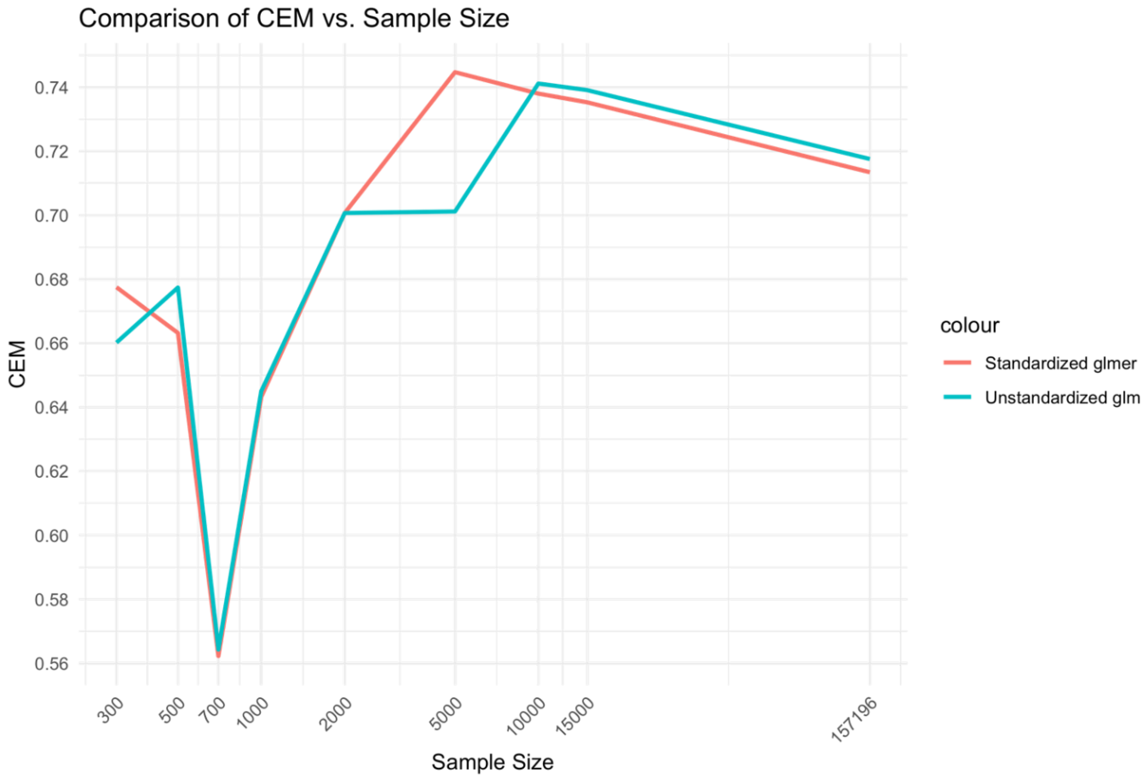
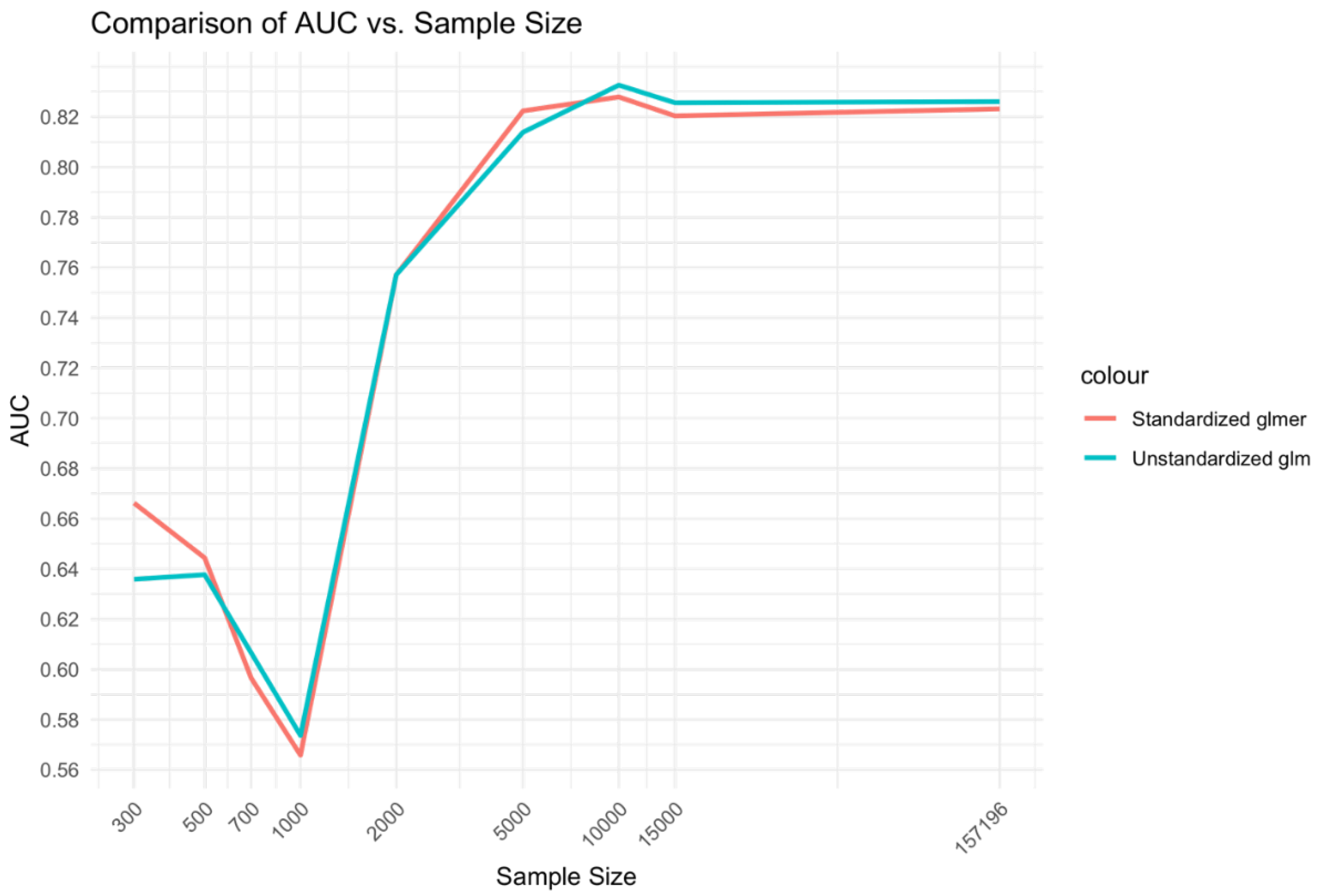
3.3.2. Unstandardized Glm and Standardized Glmer Models

In the comparison between unstandardized glm and standardized̲glmer models (Error! Reference source not found.), a similar relationship was found to the Xgboost BME vs. NC models. That is, the medium range of sample sizes, 2,000-10,000 displayed higher CEM performance for the mixed effects Xgboost BME model compared to the fixed effects Xgboost NC model. However, differences between the glmer and glm model at low sample sizes 300-1000 did not demonstrate a marked difference as that observed for the Xgboost model comparisons.

While the glm and glmer models showed higher overall CEM performance compared to the Xgboost models for middle range sample sizes, the performance of Xgboost BME and NC were higher for large sample ranges. While the Xgboost BME model showed similar performance to the glm and glmer models at low sample ranges, the performance of the Xgboost NC model was substantially lower.

Figure 4. Relationship between sample size and CEM for unstandardized glm and standardized glmer models.

Figure 4. Relationship between sample size and CEM for unstandardized glm and standardized glmer models.

The relationship of sample size to AUC was similar to that of the Xgboost model comparisons but with relative advantage of the glmer over glm at low ranges and medium ranges of sample size being less prominent (Error! Reference source not found.).

Figure 5. Relationship between sample size and AUC for unstandardized glm and standardized glmer models.

Figure 5. Relationship between sample size and AUC for unstandardized glm and standardized glmer models.

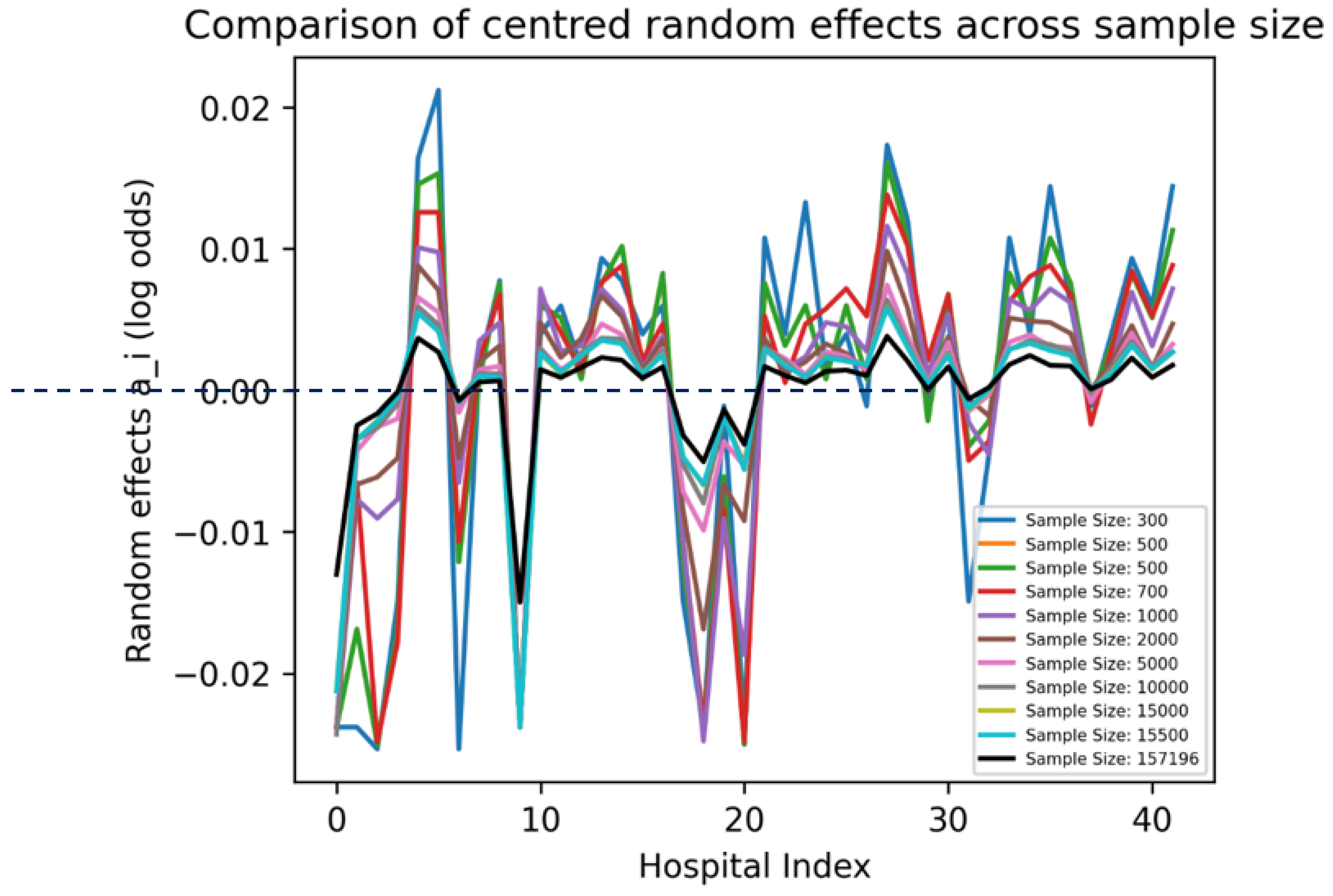
3.4. Visualization of Parameters

As sample size increased, the magnitude of the random effects decreased (Error! Reference source not found.). This concurs with earlier results which showed that the effect of the mixed effects models was larger at low – medium sample ranges compared to high sample ranges. As these random effects relate to the estimates of the model using the training set, a comparison could be made to the mortality rate of hospital 20 in the training set (Error! Reference source not found.A). It can be seen that the random effects at this point was diminished, suggesting that the high variability of hospital 20 was suppressed. This suppression may be beneficial since in the test set (Error! Reference source not found.B), the peak at hospital 20 was very small in relation to the training set.

The GLL was shown to increase as sample size increased indicating an improvement in the fit of the model (Error! Reference source not found.).

Figure 6. Unstandardized Xgboost BME: random effects (a_i) across hospitals.

Figure 6. Unstandardized Xgboost BME: random effects (a_i) across hospitals.

It was found that the proposed Xgboost BME model can reach convergence very quickly (in less than 20 iterations; Supplementary Error! Reference source not found.), and indirectly illustrates that the approach is useful.

Figure 7. Unstandardized Xgboost BME: GLL across different sample sizes.

Figure 7. Unstandardized Xgboost BME: GLL across different sample sizes.

Figure S 1. The objective function plot based on GLL for unstandardised Xgboost BME model.

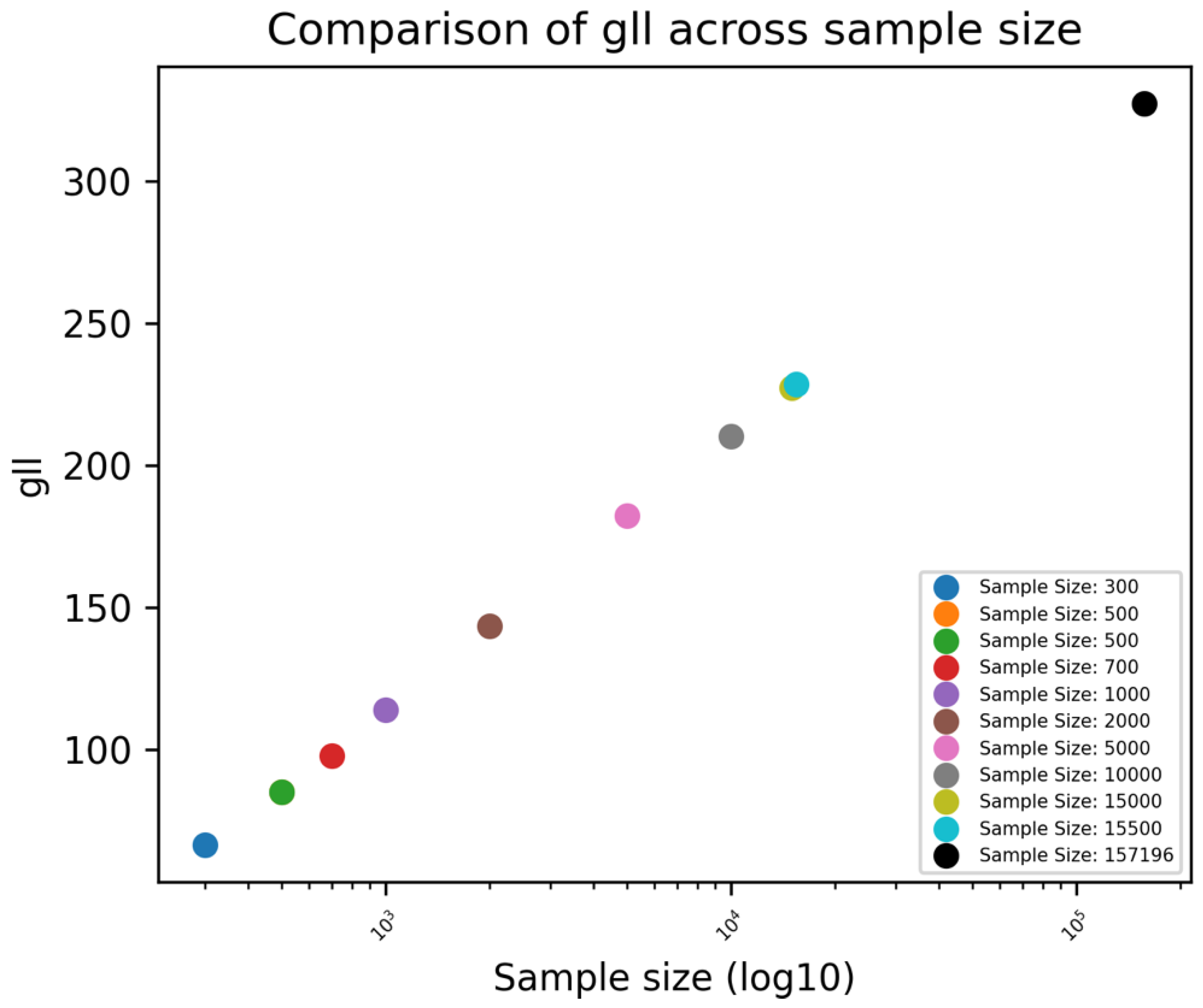
Figure S 1. The objective function plot based on GLL for unstandardised Xgboost BME model.

4. Discussion

In this study, it was found that the performance of mixed effects machine learning models varied across different sample sizes with the tendency for higher performances in low to medium range of samples over fixed effects models. Whilst these models still demonstrated high performances with large sample sizes, the impact of random effects was diminished. The reason for this phenomenon is unclear and demands further research. One speculation is that at low sample sizes, integration of random effects has a similar effect to regularisation, reducing the effect of high variability groups and that at low sample sizes this effect is greater than that at high sample sizes.

Specifically, at low sample ranges, the performance of mixed effects Xgboost BME outperformed the fixed effects Xgboost NC model by a large margin, potentially enabling Xgboost BME to have more applicability for small datasets.

4.1. Technical Perspective

The literature review by Peter et al. found that “using machine learning on small size datasets present a problem, because, in general, the ‘power’ of machine learning in recognising patterns is proportional to the size of the dataset, the smaller the dataset, the less powerful and less accurate are the machine learning algorithms.[16]” The challenge is further exacerbated when the clinical outcome is rare, whereby the small dataset may have a non-representative outcome variable frequency. For example, in cardiac surgery where the average mortality rate is often less than 3%, the number of mortalities at the smaller sample size may be difficult to extrapolate. Common approaches for dealing with low sample sizes that have been have been proposed and implemented in the literature include data augmentation through generative adversarial networks (GANs),[17] as well as regularization, an approach that adds additional parameters or constrains to prevent overfitting.[18] These approaches include adding a dropout rate modification to neural networks or defining early stop criteria during training.

While performance was similar between mixed effects variant models at low sample ranges, it was found that the mixed effects Xgboost (BME) model demonstrated higher performance at large sample ranges, while the mixed effect Logistic regression (glmer) showed higher performance at medium sample ranges. This suggests an intricate relationship between sample size and effectiveness of mixed effects on machine learning models.

The idea of incorporating random effects in tree-based machine learning models have been considered by Ahlem et al.[13] Given many biological processes that are under study in cardiovascular medicine and beyond, their approach is likely to find application for continuous outcomes whereas the Xgboost BME may be more suited for binary outcomes for example whether the patient survives or not or experiences a post-operative complication or not.

Giora et al.’s use of Gauss Hermite Quadrature approximation for approximating the random effects in mixed effects neural networks for binary dependent variable scenarios provides the basis for extending this approximation approach to other machine learning models such as Xgboost.[12] Their approach made use of the neural network’s inherent capabilities to incorporate the random effects based negative log likelihood for binary dependent variables as the loss function. This enabled the Neural Network’s performance to surpass that of the glmer model.

While Ng et al. used the EM approach to estimate the weights of their MoE model, the method adopted for estimating the likelihood is that of a residual or restricted maximum likelihood (REML) using derivatives based maximization approaches rather than a Gauss Hermite Quadrature based approach.[11] In addition, their evaluation methods were based on the use of misclassification percentages rather than the CEM and its component metrics.

In an algorithm developed by Lu et al. to handle high dimensionality datasets, it was found that convergence could occur rapidly in under five iterations.[19] The Xgboost BME algorithm showed similar performance since convergence occurred early rather than late.

The inclusion of hospital IDs as a single fixed effects variable in the model decreases interpretability by imposing a numerical ordering on naturally nominal category values, which is not conceptually meaningful. This method could result in inaccurate readings of the effect estimates since it presupposes an ordinal link between hospital identifiers, which is not the case. One-hot encoding is an alternative technique for fixed effects coding that breaks down the hospital variable into a set of binary (0/1) indicators, each of which represents a different hospital. One-hot encoding enables direct comparisons between each hospital and a composite reference group while maintaining some interpretability. However, this strategy still reduces clinical interpretability because it compares to an abstract group without a clear clinical reference, hindering understanding of hospital-specific outcomes. The increased dimensionality expands the model's degrees of freedom, increasing the danger of overfitting, particularly in models with small sample sizes or significant variability. This can produce unstable estimates, reducing the model's generalizability and clinical value. Furthermore, the added complexity of numerous hospital-specific parameters presents substantial challenges for clinicians, who may struggle to extract clear, actionable insights from these as separate variables. As a result, despite its statistical precision, this technique ultimately limits practical interpretation in clinical contexts.

The binary outcome mixed effects Xgboost (BME) model accounts for random effects changes in hospital performance while remaining interpretable. This approach allows for a assessment of how much each hospital's results deviate from the general average after controlling for other factors, By including random intercepts, the model captures hospital-specific variations and quantifies the variance attributable to each hospital allowing inter-hospital comparisons.

4.2. Relevance to Clinical Practice

4.2.1. Cardiac Surgery Perspective

Random effects modelling can be applied into day to day clinical practice. For instance, several studies have assessed the effects of regional/national level variations in treatment interventions while accounting for patients characteristics and their socioeconomic profiles.[28], [29] By using an random effects approach, this can reduce the chance of overfitting that would occur by analysing individual regions/hospitals separately. Furthermore, integration with machine learning approach could enhance predictive accuracy while retaining interpretability.

The potential use case of the XGBoost BME model for pediatric congenital heart surgery data is especially relevant considering the challenges of small sample sizes in this clinical context.[20] Paediatric congenital heart surgery frequently involves heterogeneous and complex patients, making massive dataset collection challenging due to the rarity of problems, variety in techniques, and specialized nature of care. Traditional statistical models may struggle to perform well on these small datasets, resulting in incorrect predictions and limited clinical utility.

Subject to ethical approval applications, the outcome monitoring after cardiac procedure in congenital heart disease (OMACp) or a similar congenital heart disease dataset could be analysed,[20] as these datasets capture the clinical complications and procedural variances encountered in paediatric patients. Random effects such as the site of catheterization or surgical center can be integrated into the model to account for inter-site variability, further enhancing the robustness of predictions.

4.2.2. Cardiology Perspective

Random effects models are reported in the literature to be beneficial for bias reduction through better identification of patient heterogeneity (e.g., patients with different responses to drug treatment).[21] They may be advantageous for obtaining repeated patient measures,[22] improving generalizability,[21] and increasing the predictive accuracy of ECG analyses for enhanced patient outcomes. Xgboost BME could also have an application for prediction tasks in heart rate variability (HRV) studies. A large portion of early work done in this area (especially for congestive heart failure (CHF)) adopted tree-based algorithms to deploy their models due to the interpretability of these models.[23], [24], [25] HRV is the time intervals between consecutive heartbeats. In healthy subjects, these time intervals can be highly variable. This is however not the case in patients with diseased hearts where HRV measures are depressed. Essentially, higher values of HRV indicate healthier hearts. The presence of random effects in HRV measures can be due to lifestyle factors, individual differences, types of devices used for HRV measurements, differences in conditions under which HRV is measured (e.g., physical activity, time of day, posture, stress level, age categories, etc.), and variation across different experimental study conditions. Xgboost BME could be used to account for these differences in variability that coexist within different levels of HRV data hierarchy. HRV measures are obtained from electrocardiogram (ECG) signals, and they exist in the time, frequency and non-linear domains. Xgboost BME could have utility in improving prediction tasks in these domains since ECG signals simulate the presence of random effects across the different domains, thus making more accurate and personalised interpretations possible. Xgboost BME could also enhance the extraction of ECG-related intra-subject correlations that capture individual-specific baseline ECG characteristics, and account for individual variability across multiple sites and devices.[26], [27]

5. Future work and Limitations

Although Xgboost BME hold potential for improved performance over many of these scenarios, more research is needed to determine how it can be used to better understand data distribution patterns, address sample size issues, interpret complex results, reduce the effect of outliers or influential data points on estimates of heterogeneity, and decrease computational complexities and explainability associated with large datasets or complex hierarchical structures. This then leads to the question of the efficacy of adopting nested random effects for model improvement. In this scenario, ranges of one grouping variable are completely associated with specific levels of another grouping variable to account for the structure and size of the sample data. Models incorporating this approach have been proposed in the literature to improve the accuracy and interpretability of predictions by capturing variability at different levels of data hierarchy.[30] The Xgboost algorithm is hierarchical in nature and can naturally handle nested data, but may potentially lead to increased model complexity, making the model too complicated for clinicians to understand. Several ways to address this issue have also been proposed. In the design and deployment of nested random effects models, strategies focusing on model simplicity (adopting simple models that adequately represent the data and use of appropriate model selection criteria),[31] clarity (defining clear hierarchical structures in the data by combining or collapsing levels and/or evaluating the need for each nesting level),[32], [33] and clinical relevance (using visualization and diagnostics tools to assess the distribution of random effects) are recommended.[34], [33] Wherever possible, model interpretation is to be prioritized over model fit. Also, when communicating with clinicians, simple technical language and avoidance of statistical jargon is advised when describing the model to help clinicians grasp the impact of variability between different patient groups and to ensure they understand and use the results effectively.

Some existing use of nested design models in healthcare settings include modelling the correlation between repeated measures taken from the same individual over time in longitudinal studies,[35] evaluation of variability in treatment effects in patients nested across several clinical trial centres,[36] robust estimation of randomised clinical trial effect sizes through efficient sampling,[37] and optimized estimations of overall effects of study outcomes.[38]

Many of the above mentioned aspects were out of the scope of this study. However, future work on the Xgboost BME model could incorporate some of the methods and algorithms used in the cited studies.

6. Conclusion

In this study, a binary outcome mixed effects algorithm for ensemble tree machine learning models has been presented. Performance gains over fixed effects models and traditional glm/glmer models demonstrated a complex sample size dependent relationship that deserves further research in future studies. These findings suggest that integrating mixed effects into machine learning models can enhance their applicability in clinical settings and will guide the choice of model used per study in accordance with their sample size.

References

- S. S et al., ‘Comparison of Machine Learning Techniques in Prediction of Mortality following Cardiac Surgery: Analysis of over 220,000 patients from a Large National Database’, European journal of cardio-thoracic surgery : official journal of the European Association for Cardio-thoracic Surgery, Aug. 2023. [CrossRef]
- T. Dong et al., ‘Performance Drift in Machine Learning Models for Cardiac Surgery Risk Prediction: Retrospective Analysis’, JMIRx Med, vol. 5, no. 1, p. e45973, Jun. 2024. [CrossRef]
- T. Dong et al., ‘Cardiac surgery risk prediction using ensemble machine learning to incorporate legacy risk scores: A benchmarking study’, DIGITAL HEALTH, vol. 9, p. 20552076231187605, Jan. 2023. [CrossRef]
- N. K. Kumar, G. S. Sindhu, D. K. Prashanthi, and A. S. Sulthana, ‘Analysis and Prediction of Cardio Vascular Disease using Machine Learning Classifiers’, in 2020 6th International Conference on Advanced Computing and Communication Systems (ICACCS), Mar. 2020, pp. 15–21. [CrossRef]
- P. Tiwari, K. L. Colborn, D. E. Smith, F. Xing, D. Ghosh, and M. A. Rosenberg, ‘Assessment of a Machine Learning Model Applied to Harmonized Electronic Health Record Data for the Prediction of Incident Atrial Fibrillation’, JAMA Network Open, vol. 3, no. 1, pp. e1919396–e1919396, Jan. 2020. [CrossRef]
- Mehrtash, W. M. Wells, C. M. Tempany, P. Abolmaesumi, and T. Kapur, ‘Confidence Calibration and Predictive Uncertainty Estimation for Deep Medical Image Segmentation’, IEEE Transactions on Medical Imaging, vol. 39, no. 12, pp. 3868–3878, Dec. 2020. [CrossRef]
- Huang et al., ‘Performance Metrics for the Comparative Analysis of Clinical Risk Prediction Models Employing Machine Learning. [Miscellaneous Article]’, Circulation: Cardiovascular Quality & Outcomes, vol. 14, no. 10, Oct. 2021. [CrossRef]
- E. W. Steyerberg et al., ‘Assessing the Performance of Prediction Models: A Framework for Traditional and Novel Measures’, Epidemiology, vol. 21, no. 1, pp. 128–138, Jan. 2010. [CrossRef]
- J. Allyn et al., ‘A Comparison of a Machine Learning Model with EuroSCORE II in Predicting Mortality after Elective Cardiac Surgery: A Decision Curve Analysis’, PLOS ONE, vol. 12, no. 1, p. e0169772, Jan. 2017. [CrossRef]
- M. Gregorich, S. Strohmaier, D. Dunkler, and G. Heinze, ‘Regression with Highly Correlated Predictors: Variable Omission Is Not the Solution’, Int J Environ Res Public Health, vol. 18, no. 8, p. 4259, Apr. 2021. [CrossRef]
- S.-K. Ng and G. J. McLachlan, ‘Extension of mixture-of-experts networks for binary classification of hierarchical data’, Artificial Intelligence in Medicine, vol. 41, no. 1, pp. 57–67, Sep. 2007. [CrossRef]
- G. Simchoni and S. Rosset, ‘Integrating random effects in deep neural networks’, J. Mach. Learn. Res., vol. 24, no. 1, p. 156:7402-156:7458, Mar. 2024.
- Hajjem, F. Bellavance, and D. Larocque, ‘Mixed-effects random forest for clustered data’, Journal of Statistical Computation and Simulation, Jun. 2014, Accessed: Jun. 14, 2024. [Online]. Available: https://www.tandfonline.com/doi/abs/10.1080/00949655.2012.741599.
- T. Dong et al., ‘Random effects adjustment in machine learning models for cardiac surgery risk prediction: a benchmarking study’, Jun. 12, 2023, medRxiv. [CrossRef]
- T. Dong et al., ‘Deep recurrent reinforced learning model to compare the efficacy of targeted local versus national measures on the spread of COVID-19 in the UK’, BMJ Open, vol. 12, no. 2, p. e048279, Feb. 2022. [CrossRef]
- P. Kokol, M. Kokol, and S. Zagoranski, ‘Machine learning on small size samples: A synthetic knowledge synthesis’, Sci Prog, vol. 105, no. 1, p. 00368504211029777, Feb. 2022. [CrossRef]
- J. Marin, ‘Evaluating Synthetically Generated Data from Small Sample Sizes: An Experimental Study’, Jan. 21, 2023, arXiv: arXiv:2211.10760. [CrossRef]
- S. Lutakamale and Y. Z. Manyesela, ‘Machine Learning-Based Fingerprinting Positioning in Massive MIMO Networks: Analysis on the Impact of Small Training Sample Size to the Positioning Performance’, SN COMPUT. SCI., vol. 4, no. 3, p. 286, Mar. 2023. [CrossRef]
- G. Lu, B. Li, W. Yang, and J. Yin, ‘Unsupervised feature selection with graph learning via low-rank constraint’, Multimed Tools Appl, vol. 77, no. 22, pp. 29531–29549, Nov. 2018. [CrossRef]
- M. Baquedano et al., ‘Outcome monitoring and risk stratification after cardiac procedure in neonates, infants, children and young adults born with congenital heart disease: protocol for a multicentre prospective cohort study (Children OMACp)’, BMJ Open, vol. 13, no. 8, p. e071629, Aug. 2023. [CrossRef]
- H. Schmid, P. C. Stark, J. A. Berlin, P. Landais, and J. Lau, ‘Meta-regression detected associations between heterogeneous treatment effects and study-level, but not patient-level, factors’, Journal of Clinical Epidemiology, vol. 57, no. 7, pp. 683–697, Jul. 2004. [CrossRef]
- A. Cook, S.-Y. Oh, and M. V. Pusic, ‘Accuracy of Physicians’ Electrocardiogram Interpretations’, JAMA Intern Med, vol. 180, no. 11, pp. 1–11, Nov. 2020. [CrossRef]
- L. Pecchia, P. Melillo, M. Sansone, and M. Bracale, ‘Heart Rate Variability in healthy people compared with patients with Congestive Heart Failure’, in 2009 9th International Conference on Information Technology and Applications in Biomedicine, Nov. 2009, pp. 1–4. [CrossRef]
- L. Pecchia, P. Melillo, M. Sansone, and M. Bracale, ‘Discrimination power of short-term heart rate variability measures for CHF assessment’, IEEE Trans Inf Technol Biomed, vol. 15, no. 1, pp. 40–46, Jan. 2011. [CrossRef]
- P. Melillo, R. Fusco, M. Sansone, M. Bracale, and L. Pecchia, ‘Discrimination power of long-term heart rate variability measures for chronic heart failure detection’, Med Biol Eng Comput, vol. 49, no. 1, pp. 67–74, Jan. 2011. [CrossRef]
- M. Putnikovic, Z. Jordan, Z. Munn, C. Borg, and M. Ward, ‘Use of Electrocardiogram Monitoring in Adult Patients Taking High-Risk QT Interval Prolonging Medicines in Clinical Practice: Systematic Review and Meta-analysis’, Drug Saf, vol. 45, no. 10, pp. 1037–1048, Oct. 2022. [CrossRef]
- R. C. Brindle, A. T. Ginty, A. C. Phillips, and D. Carroll, ‘A tale of two mechanisms: a meta-analytic approach toward understanding the autonomic basis of cardiovascular reactivity to acute psychological stress’, Psychophysiology, vol. 51, no. 10, pp. 964–976, Oct. 2014. [CrossRef]
- N. Stoller et al., ‘Large regional variation in cardiac closure procedures to prevent ischemic stroke in Switzerland a population-based small area analysis’, PLoS One, vol. 19, no. 1, p. e0291299, Jan. 2024. [CrossRef]
- C. Schenker et al., ‘Regional variation and temporal trends in transcatheter and surgical aortic valve replacement in Switzerland: A population-based small area analysis’, PLoS One, vol. 19, no. 1, p. e0296055, Jan. 2024. [CrossRef]
- R. J. Sela and J. S. Simonoff, ‘RE-EM trees: a data mining approach for longitudinal and clustered data’, Mach Learn, vol. 86, no. 2, pp. 169–207, Feb. 2012. [CrossRef]
- B. E. Ankenman, A. I. Avilés, and J. C. Pinheiro, ‘Optimal Designs for Mixed-Effects Models with Two Random Nested Factors’, Statistica Sinica, vol. 13, no. 2, pp. 385–401, 2003.
- T. Snijders and R. Bosker, ‘Multilevel Analysis: An Introduction to Basic and Advanced Multilevel Modeling’. https://lst-iiep.iiep-unesco.org/cgi-bin/wwwi32.exe/[in=epidoc1.in]/?t2000=013777/(100), Jan. 1999.
- Bates, M. Mächler, B. Bolker, and S. Walker, ‘Fitting Linear Mixed-Effects Models Using lme4’, Journal of Statistical Software, vol. 67, pp. 1–48, Oct. 2015. [CrossRef]
- F. Zuur, E. N. Ieno, N. J. Walker, A. A. Saveliev, and G. M. Smith, ‘Mixed Effects Modelling for Nested Data’, in Mixed effects models and extensions in ecology with R, A. F. Zuur, E. N. Ieno, N. Walker, A. A. Saveliev, and G. M. Smith, Eds., New York, NY: Springer, 2009, pp. 101–142. [CrossRef]
- D. J. Bauer, D. M. McNeish, S. A. Baldwin, and P. J. Curran, ‘Analyzing nested data: Multilevel modeling and alternative approaches’, in The Cambridge handbook of research methods in clinical psychology, in Cambridge handbooks in psychology. , New York, NY, US: Cambridge University Press, 2020, pp. 426–443. [CrossRef]
- B. Fernández-Castilla, L. Jamshidi, L. Declercq, S. N. Beretvas, P. Onghena, and W. Van den Noortgate, ‘The application of meta-analytic (multi-level) models with multiple random effects: A systematic review’, Behav Res, vol. 52, no. 5, pp. 2031–2052, Oct. 2020. [CrossRef]
- B. Rasouli et al., ‘Combining high quality data with rigorous methods: emulation of a target trial using electronic health records and a nested case-control design’, BMJ, vol. 383, p. e072346, Dec. 2023. [CrossRef]
- J. P. A. Ioannidis and H.-O. Adami, ‘Nested Randomized Trials in Large Cohorts and Biobanks: Studying the Health Effects of Lifestyle Factors’, Epidemiology, vol. 19, no. 1, p. 75, Jan. 2008. [CrossRef]
Disclaimer/Publisher’s Note: The statements, opinions and data contained in all publications are solely those of the individual author(s) and contributor(s) and not of MDPI and/or the editor(s). MDPI and/or the editor(s) disclaim responsibility for any injury to people or property resulting from any ideas, methods, instructions or products referred to in the content. |
© 2024 by the authors. Licensee MDPI, Basel, Switzerland. This article is an open access article distributed under the terms and conditions of the Creative Commons Attribution (CC BY) license (http://creativecommons.org/licenses/by/4.0/).
Copyright: This open access article is published under a Creative Commons CC BY 4.0 license, which permit the free download, distribution, and reuse, provided that the author and preprint are cited in any reuse.