
Submitted:
05 September 2024
Posted:
09 September 2024
You are already at the latest version
Abstract
In small data set learning, obtaining a large number of training samples from the source class for transfer learning is a challenge for fine-grained visual classification. Based on the fact that fine-grained concepts can be learned with very few samples, we use very few labeled samples (for example, three) in each category. However, due to the difficulty in distinguishing the subtle differences between fine-grained images, we propose a local structure information extraction method of SDFGVC based on spatial frequency features. The proposed learning module enhances the ability of the network to find significant regions and shows excellent performance in experiments on six datasets.
Keywords:
Local structure information(LSI)
; spatial frequency domain features(SFD)
; fine-grained visual classification (FGVC)
; small dataset fine-grained visual classification (SDFGVC)
1. Introduction
Image classification is one of the key problems in handling machine vision tasks. In particular, for computers, accurately classifying fine-grained images (FGVC) is a huge challenge. With the development of deep neural networks, the learning ability for subtle differences between objects is also gradually improving. For example, references such as [1,2,3,4,5,6,7,8,9,10,11,12] can accurately classify the differences between objects with high similarity. In FGVC, multiple benchmark datasets (e.g., bird species [13], cars [14], and aircrafts [15]) have also been collected through extensive labeling to test the performance of different deep learning methods.
However, the performances of the aforementioned methods begin to fall significantly when the number of samples in the dataset becomes small [16]. Meanwhile, it is expensive to collect a huge amount of labeled data for FGVC. It is also hard to collect training examples for some rare categories (e.g., endangered species). On the other hand, humans are capable of learning stable feature representations in small image datasets for dealing with FGVC tasks [17]. Inspired by this ability, in this work, we study how to make the network to learn discriminative information in each input image as accurately as possible, so that it can perform FGVC tasks with small datasets.
Visual task [18,19] largely depends on extracting local structure information (LSI) from input images, usually using various techniques such as first-order and second-order [20,21]) derivatives. In images, information of different attributes is useful for classification. For example, frequency domain information can provide features regarding image texture, etc., while spatial domain information contains the spatial positional relationship of images. At present, few people consider the local feature structure information of images simultaneously from the spatial and frequency domains. This paper starts from the frequency and spatial domains and extracts the local structure features of images from the frequency and spatial domains respectively.
In addition, image data augmentation methods such as lighting changes [22], colorization [23], rotations [24], flips [25,26], and affine transformations [27] are employed to increase data diversity and help the network learn discriminative features from images. However, existing augmentation techniques focus on increasing image diversity but cannot effectively guide the network to accurately extract local structure information from the spatial frequency domain in different fine-grained visual classification tasks. Neglecting careful consideration of local structure information extraction and local structure feature description in fine-grained visual classification methods [7,8,9,10,11,12] may lead to suboptimal performance, especially in cases where the number of samples per category in small datasets is limited.
In this work, we propose a new learning method of spatial-frequency domain local structure information features (LSI-SFD) based on fine-grained visual classification (SDFGVC). We not only extract significant local structural features in multiple directions in the spatial domain, but also obtain enhanced local structural features in multiple directions in the frequency domain after filtering. By obtaining local structural feature information in different attribute spaces, our method can more accurately locate the salient regions with classification ability in the image. At the same time, since we introduce the frequency domain and perform noise suppression in the frequency domain information, we can effectively suppress noise interference and greatly improve the classification accuracy.
This work mainly includes the following five aspects. First, taking the extraction of spatial-frequency domain local structure features as an example, it illustrates how to extract local structure features from input images in multiple directions. Second, a novel LSI-SFD learning method for SDFGVC is proposed. Third, the performance of this method on multiple small datasets is always superior to that of many advanced benchmark algorithms. Fourth, experimental results show that embedding other algorithms into this framework can significantly improve detection accuracy. Fifth, applying the method proposed in this paper to related tasks can also achieve good results.
2. Related Work
In this section, we briefly review the existing FGVC and SDFGVC methods.
2.1. Fine-Grained Visual Classification
The key problem of fine-grained visual classification (FGVC) is to enable the network to focus on regions in images that have significant classification ability. Existing FGVC methods can be roughly divided into two groups. The first group of methods [1,2,3,4,5,6] utilize various additional annotation information, such as bounding boxes, metadata, or partial annotation mechanisms to locate significant parts. Subsequently, classification is performed according to the structural information of objects from the selected regions.
The second group of methods [7,8,9,10,11,12] intend to optimize the neural network structure for locating salient regions. Zhou et al. [7] proposed a fine-grained visual classification framework that incorporates multiple discriminant parts and multi-layer features. By focusing on the most discriminating parts and masking them, the network is encouraged to explore other discriminating parts and combine shallow and deep features to enrich the local details in the discriminating features. Xu et al. [8] propose a novel internally integrated learning converter for FGVC that treats all heads of each ViT layer as weak learners and uses attention maps and spatial relational voting to characterize the labeling of discriminant regions across layers. In order to effectively mine cross-layer features and suppress noise, introduce cross-layer refinement module for extracting fine features. Cui and Hui [9] propose a dual-dependency attention converter model designed to address complex global dependency modeling challenges in visual tasks. In order to improve the quality of semantic modeling and reduce the computational cost, the model decomposes the global token interaction into two paths, namely, the location-dependent and semantic-dependent attention paths. An et al. [10] proposed a multi-scale network of progressive multi-granularity attention to address the challenges of FGVC, especially the subtle differences between classes. Through multi-granularity and multi-scale information exploration, the network uses progressive training and multi-granularity attention module to locate key discriminant regions, and uses multi-scale convolution module to extract discriminant features, thus avoiding the recognition confusion caused by subtle differences between classes. Among them, [7] and [10] also utilize multi-level feature information, enriching the local feature representation of the images. Shen et al. [11] to improve the robustness of deep models to noisy data, an adaptive label correction strategy is adopted to ensure effective learning with limited data. Pu et al. [12] introducing semantic information and employing data augmentation techniques, this approach translates image features along semantically meaningful directions to generate diversified samples, thereby enhancing the model’s generalization ability.
2.2. Visual Classification Based on Spatial Frequency Domain
Some existing SDFGVC methods combine approaches to capture image features in the frequency domain. In [28], research indicates that neural networks may exhibit preferences for certain frequency components during the learning process, which could affect the robustness of learned features. Therefore, introducing frequency domain information may enhance the neural network’s generalization capability. In [29], the Fast Fourier Transform (FFT) is introduced to effectively blend information in the frequency domain. The non-parametric nature and fast computation of FFT can efficiently learn interactions among features in the frequency domain, achieving good results even under limited sample conditions.
Moreover, approaches based on frequency domain selection have been proposed in [30] and [31], utilizing frequency domain information as input and combining it with CNNs structures to transform image features from spatial domain to frequency domain. Compared to traditional spatial domain approaches, frequency domain learning can achieve higher accuracy while further reducing input data volume. Research on combining spatial and frequency domain features, as seen in [32] and [33], utilizes multi-domain cross or complementary fusion methods. In the context of few shot classification problems, attention is given to both spatial and frequency domains, allowing for the extraction of structural information in both domains. Studies on fusion methods for spatial and frequency domain features indicate that effective frequency domain information has a positive impact on classification. This also highlights the complementary nature of frequency information and spatial representation, effective fusion of spatial and frequency domain features leads to better image feature representation.
2.3. Small Dataset Fine-Grained Visual Classification
The existing SDFGVC method [34,35,36,37,38,39,40] can be roughly divided into two categories [41]: meta-learning based methods [34,35,36] and metric-based learning methods [37,38,39,40]. The strategy of the meta-learning method is to train the classifier using only a small number of training samples for each class. Tang et al. [34] propose an efficient bidirectional pyramid architecture that enhances the internal representation of features by aggregating features from a multi-scale feature pyramid and a multi-level attention pyramid. Zhang et al. [35] proposed a double helix model based on Transformer. The model first achieves better cross-image interaction in semantically relevant local object regions, and then enhances the extraction features of semantically relevant local regions found in each branch, thereby enhancing the model’s ability to distinguish subtle feature differences in fine-grained objects. Satoshi et al. [36] proposed a meta-image enhancement network that combines the generated image with the original image, thereby enabling the generated "hybrid" training image to improve one-shot learning.
A strategy based on metric learning methods is to learn a set of functions that transform the test sample into an embedded space. The test sample can then be classified according to a given metric (for example, nearest neighbor [42] or deep nonlinear metric [43]). Zhang et al. [37] used Earth Mover Distance as an indicator to calculate the structural distance between dense image representations to determine image correlation. Wertheimer et al. [38]reformulated the small-sample classification as a reconstruction problem in potential space and proposed a feature reconstruction network. A new small sample classification mechanism is designed, that is, directly reconstruct from support set samples to query set samples, which can greatly increase the difference between classes and improve the classification performance. In order to alleviate low inter-class variation and high intra-class variation, Wu et al. [39] proposed a bidirectional feature reconstruction network, introduced self-attention mechanism to reconstruct images, used support sets to reconstruct query sets to increase inter-class differences, and further used query sets to reconstruct support sets to reduce intra-class differences. However, most of the existing few-shot image classification methods only focus on the modeling of global image features or local image patches, and ignore the global-local interaction. Sun et al. [40] propose a new approach called GL-ViT, which designs a feature extraction module to compute the interaction between global representation and local patch embedding, combining global and local features to make the most of small samples for image classification.
3. Proposed Method
In this section, we first clarify how to correctly extract the spatial-frequency domain local structure information feature (LSI-SFD). Then, a novel local structure information (LSI) learning method for fine-grained visual classification (SDFGVC) is proposed. As shown in Figure 1, the framework consists of three modules: local structure information preprocessing, backbone network, and classification network. Next, the reason why the proposed algorithm can effectively function will be explained, as well as how our proposed framework enables the backbone network to have the ability to obtain accurate LSI-SFD from each input image in order to learn discriminative information from salient regions.
3.1. LSI Extraction
The extraction of Local Structural Information (LSI) [44,45] from input images has a profound impact on the effectiveness of subsequent classification tasks in computer vision and image processing. In images, basic structural elements include corners, edges, and blobs. Typically, first-order differentials are widely cited in literatures such as [19,46,47,48] and are widely used in edge [49] and corner identification [50,51], while second-order differentials [52,53] are common in blob detection. In this paper, local structural information in input images is extracted according to the different response values generated by the derivatives of different structures in images in different directions of first-order and second-order anisotropic Gaussian filters. Parameters such as scale and anisotropic factors are all set correspondingly to .
In the test image “Building” depicted in Figure 2(a), where a corner, an edge point, and a blob are denoted by symbols ‘’, ‘□’, and ‘◯’ respectively. In Figure 2(b) shows the response value of the FOAGDD of the corner point. Figure 2(b) and(c) show that the directional derivatives of the T-shaped corner and the edge are different. After the lighting changes, the response values of the corner and the edge change, but in the horizontal and vertical directions, they are consistent with when there is no change, which is not conducive to image classification learning. These observations align with prior representations of FOAGDD for corners and edges [46,48], suggesting the necessity of LSI extraction along multiple filter orientations. However, the response value of the SOAGDD of the blob does not change significantly. Different lighting affects the characterization and classification of local structural attributes and thus affects the extraction of LSI.
Additionally, using a test image named “Graffiti”, depicted in Figure 3(a). Here, we denote a corner, an edge point, and a blob with symbols ‘’, ‘□’, and ‘◯’ respectively. Figure 3(b), (c), and (d) showcase the FOAGDD of the corner and the edge, and the SOAGDD of the blob on the original image. Now, if we subject the original image to an image affine transformation as depicted in Figure 3(e), upon comparison with Figure 3(b), (c), and (d), it’s evident from Figure 3(f), (g), and (h) that there are significant changes in the FOAGDD of the corner and the edge, and the SOAGDD of the blob. Therefore, relying solely on LSI extraction along horizontal and vertical filter orientations fails to accurately represent the characteristics of local structural features.
From the above example, it is clear that the intrinsic properties of the local structural features of the image remain the same despite the change in illumination or deformation. For example, a FOAGDD for an edge shows only one local maximum and minimum, while a FOAGDD for a corner shows many local maximum and minimum values. In contrast, a blob’s SOAGDD appears entirely positive or negative. In addition, it is clear that fully describing different local structural features requires extracting the LSI from input images in different directions. Therefore, in FGVC and SDFGVC tasks, it is necessary to exclude iterative optimization and use different directional filters to concurrently process the extracted local structure information. Therefore, this method can accurately extract enough LSI from each input image to facilitate the analysis of different significant regions and improve the efficacy of FGVC and SDFGVC.
3.2. Information Preprocessing
In order to help the backbone network accurately learn salient local regions of objects and the overall structure of objects, the original image I first undergoes a DCT transformation to convert the image from the spatial domain to the frequency domain, acquiring the frequency information of the image. The frequency information of the image is then subjected to low-pass filtering to remove some high-frequency noise interference, followed by an IDCT to transform the low-frequency information of the image back to the spatial domain. Subsequently, the original image and the image generated by the low-frequency information, denoted as image , are rotated with multiple angles at an interval of within the range of . This process yields a series of rotated original images (k=…,K−1) and low-frequency rotated images (k=…,K−1), which are then fed into the backbone network for training. Taking the backbone network as an example, as depicted in Figure 4, it can extract the first-order intensity variation information of each input image along horizontal and vertical filter orientations. In Figure 4(a) shows the extraction of local structural features of images in a single direction used in most methods. However, this operation can only enable the backbone network to learn part of the local information of an image in each epoch, and it may not necessarily contain the local parts with classification ability. On the contrary, the method proposed in this paper enables the network to extract the local structural features of images along multiple directions from different attribute spaces in each epoch, which can ensure that significant local features with classification ability in the image can be obtained in each epoch. As shown in "in every epoch" in Figure 4(b). Through this method, the backbone network can accurately acquire LSI from each input image in both spatial and frequency domain attribute spaces, facilitating the learning of discriminative information from salient regions.
It is worth to note that a backbone network has the ability to learn different information from each input image with data augmentation (e.g., letting the image rotate randomly each time). In this way, one may argue that as long as the number of epochs is increased during training, the network as shown in Figure 4(a) can obtain more LSI from input images with data augmentation. And then the network as shown in Figure 4(a) has the ability to achieve a similar or better classification accuracy than the network as shown in Figure 4(b). Later experiments will show that under small sample conditions, increasing the number of epochs (e.g., letting the number of epochs in Figure 4(a) be ten times that of Figure 4(b)) cannot improve the classification accuracy of the network as shown in Figure 4(a). The reason is that the LSI learned by the network as shown in Figure 4(a) is inadequate which cannot be used to accurately describe the different local structure features of an image. This is similar to the capability of a person to process information. Under the original limited amount of information, if the information that people have is inadequate, the accuracy of a person’s judgment on events is likely to be low. Furthermore, experimental comparisons illustrate that our proposed method achieves better performance when the number of training images in the dataset is limited.
3.3. Classification Network
The objects in different images of the same category usually share some similarities. In our method, the input image I is transformed into rotated images (k=…,K) and rotated images with low-frequency filtering (k=…,K) through an information preprocessing module. Then, these rotated images along with their corresponding one-vs-all fine-grained category labels are integrated into training set {,…,, and {,…,,. The two sets of images are fed into the backbone network to obtain their corresponding feature maps in two different attribute spaces{,…, and {,…, , which are fused using learned weights. Subsequently, the fused feature maps are processed by an adaptive average pooling layer and a fully connected layer in the classification network to obtain the classification distribution {,…,. In this way, the classification loss is defined as
where C represents the image set for training.
In our framework, the classification network is trained through end-to-end transfer learning, enabling the network to accurately learn the significant local regions and overall structures of objects. The entire framework of LSI-SFD learning is illustrated in Figure 1. The information preprocessing module assists the backbone network in accurately learning the LSI of different types of objects in both spatial and frequency domains from each input image. The classification network helps the network learn the local structural information of objects from different attributes. In this way, LSI-SFD learning possesses the capability to accurately learn the attributes of different objects in images, thereby achieving better performance in SDFGVC.
4. Experiments
In this section, the datasets and detailed experiment settings for SDFGVC are firstly introduced. Secondly, the impact of information preprocessing on the performance of the proposed method is illustrated. Furthermore, the impact of the number of epochs for classification accuracy is illustrated. Thirdly, the proposed LSI-SFD learning method is compared with eight state-of-the-art methods. Fourthly, embedding other algorithms into our proposed framework, their corresponding detection accuracies are presented.
4.1. Experiment Setting
In this experiment, three training samples and three test samples in each category are randomly selected from six standard image datasets (i.e.,Cotton [54], Oxford Flower (FLO) [55], CUB-200-2011 (CUB) [13], Standford Cars (CAR) [14], FGVC-Aircraft (AIR) [15], and plant disease (PD) [56]) for evaluating the classification accuracy of the proposed method in comparison with the state-of-the-art benchmark methods (VGG-16 [57], ResNet50 [58], NTS-Net [59], fast-MPN-Cov [60], DCL [26], Cross-X [61], MOMN [62], ACNet [25], and fingerprints vitality detection (FVD) [63]). The codes for these eight methods are provided by their authors and the classification labels of the image datasets are the only annotations used for training in our experiments. The proposed method is implemented in PyTorch using a 3.50 GHz CPU with 128 GB memory and eight NVIDIA TITAN Xp with 12 GB memory.
The cotton dataset [54] contains 80 cotton leaf categories. The FLO dataset [55] contains 102 classes of flowers. The CUB dataset [13] contains 200 classes of birds. The CAR dataset [14] contains 196 classes. The AIR dataset [15] contains 100 classes. The PD dataset [56] contains 38 plant disease categories. For each category, it contains 6 images. For the six images, we follow the setting of for training and testing. It means that, for each category, a images are utilized for training and b images are employed for testing. In this experiment, the numbers of a and b are set to , and , respectively.
In our method, ResNet-50 [58] is used as a backbone network. The input images are padded to squares before being resized to the size of pixels, and then they are randomly rotated and cropped to pixels. All the methods are trained for 180 epoches using stochastic gradient descent with a batch size of 16. The learning rate is 0.001 initially and then decreases by a factor of 10 every 60 epochs. The benchmark methods are implemented using the optimal settings as reported in their papers with careful fine-tuning.
4.2. Parameter Settings
In this subsection, we first use input image sets in the spatial domain and frequency domain to test the accuracy of the proposed method. From this experiment, we find that the number of rotations of images in different directions in the spatial domain and frequency domain has a great impact on performance, as shown in Figure 5. With , the proposed method achieves the best performance on the cotton dataset [54]. With , the accuracy of the proposed method is the worst. The reason is that input images with two rotation directions in the spatial domain and frequency domain cannot enable the network to learn sufficient local self-similarity (LSI). At the same time, it can be observed that the accuracy of the image set composed of six images in the spatial domain and frequency domain is more stable and relatively better than that of image sets composed of other numbers of images in the spatial domain and frequency domain. The reason is that the image set composed of six images in the spatial domain and frequency domain can provide more LSI to the network. Based on the above analysis, in the subsequent experiments, the proposed method uses an input image set composed of six images in the spatial domain and frequency domain.
Then, we use the input image set composed of six images in the spatial domain and frequency domain respectively to test the accuracy of our proposed method on six other small datasets. Table 1 shows the classification accuracy on the cotton, airplane, flower, bird, car, and plant disease datasets under different combinations of image rotations with six directions. It can be found from the table that the accuracy of our algorithm is stable in six input images with different rotation directions in the spatial domain and frequency domain. Then, the best accuracy of the proposed method in each dataset will be selected for performance comparison with other algorithms.
In the following, we discuss the impact of the number of epochs for the accuracy of SDFGVC. Take the cotton dataset as an example, the classification accuracies of the four methods (VGG-16 [57], ResNet50 [58], DCL [26], and proposed method with two image rotation directions ) under 1800 epochs and the proposed method with six image rotation directions under 180 epochs are shown in Figure 6. It can be seen from Figure 6 that at the beginning, with the increase of epochs, the accuracies of the four algorithms have been increasing. When the epoch reaches about 120, the accuracies of the five algorithms on the cotton dataset become stable. It can also be found from Figure 6 that when the epoch is increased to 1,800 with data augmentation, the accuracies of the four algorithms (VGG-16 [57], ResNet50 [58], DCL [26], and proposed method with two image rotation directions ) cannot reach the accuracy of the proposed method with six image rotation directions .
4.3. Experiment Results
The results on the selected six small datasets from Cotton, CUB-200-2011, Standford Cars, FGVC-Aircraft, Oxford Flower, and plant disease datasets are illustrated in Table 2 and Table 3. It can be observed from Table 2 and Table 3 that our proposed method achieves much better performance than the benchmark methods with small datasets. The reason is that our proposed method has the ability to allow the network to learn more LSI of features from each input image. Under this way, our proposed method has better ability to depict the properties of different features in images. Furthermore, it can be found that the accurate extraction of LSI of different features in images has a more significant impact on the performance of SDFGVC.
Based on the Resnet-50, we also compared our method with the existing image data augmentation techniques (i.e., lighting changes [22], colorizing images [23], image rotations [24], image flips [25,26], and image affine transformations [27]) on seven small datasets with and . The results are shown in Table 4. It can be found from Table 4 that our proposed method achieves the best performance.
Furthermore, embedding three algorithms (NTS-Net [59], fast-MPN-Cov [60], and DCL [26]) into our proposed framework with six image rotation directions , , , , , their corresponding accuracies on two small datasets (Cotton and CUB) are summarized in Table 5. It can be found from Table 5 that the accuracies of the three methods have improved significantly.
5. Application
In this subsection, the proposed network is applied for performing change detection on SAR image. The SAR images used in this application section are sourced from the geographic image information of Zhongchi Town, Shiquan County, Ankang City, Shaanxi Province, China, at two time points in 2021.
5.1. Patch Data and Preprocessing
Due to factors such as the patch information being collected in 2017 and considerations of SAR shooting angles, it is necessary to correct and match the positions of the 2021 SAR image with the patches to ensure accurate correspondence. The irregular polygon edge coordinates are found in the mask image, and new mask regions are created using these coordinates. Finally, this region is overlaid with the 2021 SAR image of Zhongchi Town to segment the farmland patch areas, resulting in 1773 patch areas.
Considering the varying size and shape of irregular patches, direct classification is difficult. Therefore, while segmenting irregular patches, their minimum bounding rectangles are also segmented to obtain two types of datasets: regular patch data and irregular patch data. Subsequently, combining manual judgment of whether the patches are farmland areas, corresponding labels are generated for inference to calculate accuracy.
5.2. Data Training
To conduct model training and evaluation, it is necessary to construct training, validation, and testing datasets. These datasets are obtained by segmenting the original SAR images, with each image sized at pixels. After manual judgment, the images are classified into two categories: farmland and non-farmland.
Specifically, we constructed a training dataset consisting of 2148 images, as well as separate validation and testing datasets, each containing 460 images.In the training dataset, training samples are used for model learning and parameter adjustment. Validation data are used to assess the model’s performance and conduct hyperparameter selection and adjustment. Testing data are then used to finally evaluate the model’s generalization ability and accuracy.Through such dataset partitioning and utilization, the proposed model’s performance in farmland change detection tasks can be comprehensively evaluated, providing reliable metrics for its performance.
5.3. Inference and Change Detection
In the process of change detection using random cropping method, it refers to randomly cropping the patch area during change detection of each patch. Due to the irregular shape of the patches and the use of white filling for rectangles, the shapes vary and cannot be directly used for detection. Therefore, when segmenting the patches from the original image, the minimum inscribed rectangle of the irregular patches needs to be found to segment out regular images. When predicting the patches, both regular and irregular patch loaders are created. Non-white areas of irregular patches are identified, and the center point of the cropping box is determined using random numbers. Since the sizes of regular and irregular patches are the same, the center point position is corresponded in the irregular image and checked if it’s on the boundary. If the center point position is satisfied and a image block can be cropped, the image block is predicted using the LSI-SFD method, and the occurrence of changes is determined based on the predicted category.
5.4. Change Detection Result
Using the 2021 SAR image of Zhongchi Town and the ArcGIS vector map information of permanent farmland in Zhongchi Town in 2017, all farmland patches were segmented. By designing a random cropping method combined with the LSI-SFD method, rapid and accurate change detection of farmland was achieved. Due to the slight displacement of the patches in 2021, the types, quantities, and prediction results of the patches can be inferred from Table 6.
According to Table 6, there were 1773 patches of farmland in Zhongchi Town in 2021. By segmenting and classifying image patches across multiple models, it can be seen from the detection results that when using the method proposed in this paper, LSI-SFD, for change detection of permanent farmland in Zhongchi Town, it is able to quickly and accurately classify patch information for detection.
6. Conclusion
The paper focuses on addressing the challenge of small dataset fine-grained classification problems by exploring LSI-SFD from a few labeled examples. Firstly, we elucidate how to accurately extract LSI from each input image, enabling the network to accurately describe the properties of different features in images across various spatial dimensions. Secondly, we conduct a detailed analysis of the limitations of existing data augmentation techniques. Thirdly, we propose a novel LSI-SFD learning framework for SDFGVC. Fourthly, the proposed method demonstrates superior performance on six small datasets. Fifthly, by integrating other algorithms into our proposed framework, their detection accuracy can be significantly improved.
Moreover, we applied the LSI-SFD method proposed in this paper to complete change detection tasks on SAR images of Zhongchi Town in 2021 with limited samples. By transforming change detection into a binary classification problem using classification, compared to existing image classification methods, the LSI-SFD method proposed in this paper can more accurately detect and classify SAR images.
References
- Jonathan, K.; Jin, H.; Yang, J.; Fei-Fei, L. Fine-grained recognition without part annotations. IEEE Conference on Computer Vision and Pattern Recognition, 2015, pp. 5546–5555.
- Huang, S.; Xu, Z.; Tao, D.; Zhang, Y. Part-stacked CNN for fine-grained visual categorization. Conference on Computer Vision and Pattern Recognition, 2016, pp. 1173–1182.
- Berg, T.; Liu, J.; Woo Lee, S.; Alexander, M.L.; Jacobs, D.W.; Belhumeur, P.N. Birdsnap: Large-scale fine-grained visual categorization of birds. IEEE Conference on Computer Vision and Pattern Recognition, 2014, pp. 2011–2018.
- Ye, S.; Wang, Y.; Peng, Q.; You, X.; Chen, C.P. The image data and backbone in weakly supervised fine-grained visual categorization: A revisit and further thinking. IEEE Transactions on Circuits and Systems for Video Technology 2023, pp. 2–16. [CrossRef]
- Wang, H.; Liao, J.; Cheng, T.; Gao, Z.; Liu, H.; Ren, B.; Bai, X.; Liu, W. Knowledge mining with scene text for fine-grained recognition. IEEE Conference on Computer Vision and Pattern Recognition, 2022, pp. 4624–4633.
- Diao, Q.; Jiang, Y.; Wen, B.; Sun, J.; Yuan, Z. Metaformer: A unified meta framework for fine-grained recognition. arXiv preprint arXiv:2203.02751 2022.
- Zhou, P.; Pang, C.; Lan, R.; Wu, G.; Zhang, Y. Multi-discriminative Parts Mining for Fine-Grained Visual Classification. Asian Conference on Pattern Recognition, 2023, pp. 279–292.
- Xu, Q.; Wang, J.; Jiang, B.; Luo, B. Fine-grained visual classification via internal ensemble learning transformer. IEEE Transactions on Multimedia 2023, pp. 9015–9028. [CrossRef]
- Cui, S.; Hui, B. Dual-Dependency Attention Transformer for Fine-Grained Visual Classification. Sensors 2024, 24, 2337. [Google Scholar] [CrossRef] [PubMed]
- An, C.; Wang, X.; Wei, Z.; Zhang, K.; Huang, L. Multi-scale network via progressive multi-granularity attention for fine-grained visual classification. Applied Soft Computing 2023, 146, 110588. [Google Scholar] [CrossRef]
- Shen, J.; Yao, Y.; Huang, S.; Wang, Z.; Zhang, J.; Wang, R.; Yu, J.; Liu, T. ProtoSimi: label correction for fine-grained visual categorization. Machine Learning 2024, 113, 1903–1920. [Google Scholar] [CrossRef]
- Pu, Y.; Han, Y.; Wang, Y.; Feng, J.; Deng, C.; Huang, G. Fine-grained recognition with learnable semantic data augmentation. IEEE Transactions on Image Processing 2024, pp. 3130–3144. [CrossRef]
- Wah, C.; Branson, S.; Welinder, P.; Perona, P.; Belongie, S. The Caltech-UCSD Birds-200-2011 dataset. California Institute of Technology 2011. [Google Scholar]
- Krause, J.; Stark, M.; Deng, J.; Fei-Fei, L. 3D object representations for fine-grained categorization. IEEE International Conference on Computer Vision Workshops, 2013, pp. 554–561.
- Maji, S.; Rahtu, E.; Kannala, J.; Blaschko, M.; Vedaldi, A. Fine-grained visual classification of aircraft. ArXiv Preprint ArXiv:1306.5151 2013.
- Wang, Y.; Yao, Q.; Kwok, J.T.; Ni, L.M. Generalizing from a few examples: A survey on few-shot learning. ACM Computing Surveys 2020, 53, 1–34. [Google Scholar] [CrossRef]
- Schmidt, L.A. Meaning and compositionality as statistical induction of categories and constraints. PhD thesis, Massachusetts Institute of Technology, 2009.
- Shui, P.L.; Zhang, W.C. Corner detection and classification using anisotropic directional derivative representations. IEEE Transactions on Image Processing 2013, 22, 3204–3218. [Google Scholar] [CrossRef] [PubMed]
- Zhang, W.; Zhao, Y.; Breckon, T.P.; Chen, L. Noise robust image edge detection based upon the automatic anisotropic Gaussian kernels. Pattern Recognition 2017, 63, 193–205. [Google Scholar] [CrossRef]
- Li, P.; Lu, X.; Wang, Q. From dictionary of visual words to subspaces: Locality-constrained affine subspace coding. IEEE Conference on Computer Vision and Pattern Recognition, 2015, pp. 2348–2357.
- Dai, X.; Ng, J.Y.; Davis, L.S. FASON: First and Second Order Information Fusion Network for Texture Recognition. IEEE Conference on Computer Vision and Pattern Recognition, 2017, pp. 6100–6108.
- Huang, S.W.; Lin, C.T.; Chen, S.P.; Wu, Y.Y.; Hsu, P.H.; Lai, S.H. AugGAN: Cross domain adaptation with GAN-based data augmentation. European Conference on Computer Vision, 2018, pp. 718–731.
- Yoo, S.; Bahng, H.; Chung, S.; Lee, J.; Chang, J.; Choo, J. Coloring with limited data: Few-shot colorization via memory augmented networks. IEEE Conference on Computer Vision and Pattern Recognition, 2019, pp. 11283–11292.
- Feng, Z.; Xu, C.; Tao, D. Self-supervised representation learning by rotation feature decoupling. IEEE Conference on Computer Vision and Pattern Recognition, 2019, pp. 10364–10374.
- Ji, R.; Wen, L.; Zhang, L.; Du, D.; Wu, Y.; Zhao, C.; Liu, X.; Huang, F. Attention convolutional binary neural tree for fine-grained visual categorization. IEEE Conference on Computer Vision and Pattern Recognition, 2020, pp. 10468–10477.
- Chen, Y.; Bai, Y.; Zhang, W.; Mei, T. Destruction and construction learning for fine-grained image recognition. Proceedings of the IEEE Conference on Computer Vision and Pattern Recognition, 2019, pp. 5157–5166.
- Luo, C.; Zhu, Y.; Jin, L.; Wang, Y. Learn to augment: Joint data augmentation and network optimization for text recognition. Conference on Computer Vision and Pattern Recognition, 2020, pp. 13746–13755.
- Lin, S.;Zhang,Z.;Huang,Z.;Lu,Y.;Lan,C.;Chu,P.;You,Q.;Wang,J.;Liu,Z.;Parulkar,A.; others. Deep frequency filtering for domain generalization. IEEE Conference on Computer Vision and Pattern Recognition, 2023, pp. 11797–11807.
- Shi, H.; Cao, G.; Zhang, Y.; Ge, Z.; Liu, Y.; Yang, D. F 3 Net: Fast Fourier filter network for hyperspectral image classification. IEEE Transactions on Instrumentation and Measurement 2023. [Google Scholar] [CrossRef]
- Xu, K.; Qin, M.; Sun, F.; Wang, Y.; Chen, Y.K.; Ren, F. Learning in the frequency domain. IEEE conference on computer vision and pattern recognition, 2020, pp. 1740–1749.
- Lin, H.; Tse, R.; Tang, S.K.; Qiang, Z.; Pau, G. Few-shot learning for plant-disease recognition in the frequency domain. Plants 2022, 11, 2814. [Google Scholar] [CrossRef]
- Zhu, H.; Gao, Z.; Wang, J.; Zhou, Y.; Li, C. Few-shot fine-grained image classification via multi-frequency neighborhood and double-cross modulation. arXiv preprint arXiv:2207.08547 2022.
- Chen, X.; Wang, G. Few-shot learning by integrating spatial and frequency representation. 2021 18th Conference on Robots and Vision (CRV), 2021, pp. 49–56.
- Tang, H.; Yuan, C.; Li, Z.; Tang, J. Learning attention-guided pyramidal features for few-shot fine-grained recognition. Pattern Recognition 2022, 130, 108792. [Google Scholar] [CrossRef]
- Zhang, B.; Yuan, J.; Li, B.; Chen, T.; Fan, J.; Shi, B. Learning cross-image object semantic relation in transformer for few-shot fine-grained image classification. 30th ACM International Conference on Multimedia, 2022, pp. 2135–2144.
- Tsutsui, S.; Fu, Y.; Crandall, D. Reinforcing generated images via meta-learning for one-shot fine-grained visual recognition. IEEE Transactions on Pattern Analysis and Machine Intelligence 2022. [Google Scholar] [CrossRef] [PubMed]
- Zhang, C.; Cai, Y.; Lin, G.; Shen, C. Deepemd: Few-shot image classification with differentiable earth mover’s distance and structured classifiers. IEEE conference on computer vision and pattern recognition, 2020, pp. 12203–12213.
- Wertheimer, D.; Tang, L.; Hariharan, B. Few-shot classification with feature map reconstruction networks. IEEE conference on computer vision and pattern recognition, 2021, pp. 8012–8021.
- Wu, J.; Chang, D.; Sain, A.; Li, X.; Ma, Z.; Cao, J.; Guo, J.; Song, Y.Z. Bi-directional feature reconstruction network for fine-grained few-shot image classification. AAAI Conference on Artificial Intelligence, 2023, Vol. 37, pp. 2821–2829.
- Sun, M.; Ma, W.; Liu, Y. Global and local feature interaction with vision transformer for few-shot image classification. 31st ACM International Conference on Information & Knowledge Management, 2022, pp. 4530–4534.
- Ren, J.; Li, C.; An, Y.; Zhang, W.; Sun, C. Few-Shot Fine-Grained Image Classification: A Comprehensive Review. AI 2024, 5, 405–425. [Google Scholar] [CrossRef]
- Snell, J.; Swersky, K.; Zemel, R. Prototypical networks for few-shot learning. Advances in Neural Information Processing Systems, 2017, pp. 4077–4087.
- Sung, F.; Yang, Y.; Zhang, L.; Xiang, T.; Torr, P.H.; Hospedales, T.M. Learning to compare: Relation network for few-shot learning. IEEE Conference on Computer Vision and Pattern Recognition, 2018, pp. 1199–1208.
- Jing, J.; Gao, T.; Zhang, W.; Gao, Y.; Sun, C. Image feature information extraction for interest point detection: A comprehensive review. IEEE Transactions on Pattern Analysis and Machine Intelligence 2022, 45, 4694–4712. [Google Scholar] [CrossRef] [PubMed]
- Zhang, W.; Sun, C.; Gao, Y. Image intensity variation information for interest point detection. IEEE Transactions on Pattern Analysis and Machine Intelligence 2023, 45, 9883–9894. [Google Scholar] [CrossRef] [PubMed]
- Shui, P.L.; Zhang, W.C. Corner detection and classification using anisotropic directional derivative representations. IEEE Transactions on Image Processing 2013, 22, 3204–3218. [Google Scholar] [CrossRef]
- Zhang, W.C.; Shui, P.L. Contour-based corner detection via angle difference of principal directions of anisotropic Gaussian directional derivatives. Pattern Recognition 2015, 48, 2785–2797. [Google Scholar] [CrossRef]
- Zhang, W.; Sun, C. Corner detection using multi-directional structure tensor with multiple scales. International Journal of Computer Vision 2020, 128, 438–459. [Google Scholar] [CrossRef]
- Jing, J.; Liu, S.; Wang, G.; Zhang, W.; Sun, C. Recent advances on image edge detection: A comprehensive review. Neurocomputing 2022, 503, 259–271. [Google Scholar] [CrossRef]
- Jing, J.; Gao, T.; Zhang, W.; Gao, Y.; Sun, C. Image Feature Information Extraction for Interest Point Detection: A Comprehensive Review 2021. abs/2106.07929.
- Zhang, W.; Sun, C.; Breckon, T.; Alshammari, N. Discrete curvature representations for noise robust image corner detection. IEEE Transactions on Image Processing 2019, 28, 4444–4459. [Google Scholar] [CrossRef]
- Lowe, D.G. Distinctive image features from scale-invariant keypoints. International Journal of Computer Vision 2004, 60, 91–110. [Google Scholar] [CrossRef]
- Zhang, W.; Sun, C. Corner detection using second-order generalized Gaussian directional derivative representations. IEEE Transactions on Pattern Analysis and Machine Intelligence 2021, 43, 1213–1224. [Google Scholar] [CrossRef] [PubMed]
- Yu, X.; Zhao, Y.; Gao, Y.; Xiong, S.; Yuan, X. Patchy image structure classification using multi-orientation region transform. Association for the Advancement of Artificial Intelligence, 2020, pp. 12741–12748.
- Nilsback, M.; Zisserman, A. Automated flower classification over a large number of classes. Sixth Indian Conference on Computer Vision, Graphics Image Processing, 2008, pp. 722–729.
- Mohanty, S.P.; Hughes, D.P.; Salathé, M. Using deep learning for image-based plant disease detection. Frontiers in Plant Science 2016, 7, 1419. [Google Scholar] [CrossRef] [PubMed]
- Simonyan, K.; Andrew, Z. Very deep convolutional networks for large-scale image recognition. Proceedings of the International Conference on Learning Representations, 2015, pp. 770–784.
- He, K.; Zhang, X.; Ren, S.; Sun, J. Deep residual learning for image recognition. IEEE Conference on Computer Vision and Pattern Recognition, 2016, pp. 770–778.
- Yang, Z.; Luo, T.; Wang, D.; Hu, Z.; Gao, J.; Wang, L. Learning to navigate for fine-grained classification. European Conference on Computer Vision, 2018, pp. 420–435.
- Li, P.; Xie, J.; Wang, Q.; Gao, Z. Towards faster training of global covariance pooling networks by iterative matrix square root normalization. IEEE Conference on Computer Vision and Pattern Recognition, 2018, pp. 947–955.
- Luo, W.; Yang, X.; Mo, X.; Lu, Y.; Davis, L.S.; Li, J.; Yang, J.; Lim, S.N. Cross-X learning for fine-grained visual categorization. Proceedings of the IEEE International Conference on Computer Vision, 2019, pp. 8242–8251.
- Min, S.; Yao, H.; Xie, H.; Zha, Z.J.; Zhang, Y. Multi-objective matrix normalization for fine-grained visual recognition. IEEE Transactions on Image Processing 2020, 29, 4996–5009. [Google Scholar] [CrossRef]
- Impedovo, D.; Dentamaro, V.; Abbattista, G.; Gattulli, V.; Pirlo, G. A comparative study of shallow learning and deep transfer learning techniques for accurate fingerprints vitality detection. Pattern Recognition Letters 2021, 151, 11–18. [Google Scholar] [CrossRef]
Figure 1.
The overall pipeline of our proposed LSI-SFD learning framework. (1) Information preprocessing: filtering noise in the frequency domain of input images and rotating them. (2) Backbone classification network: extracting the basic feature maps. (3) Classification network: classifying images into fine-grained categories.
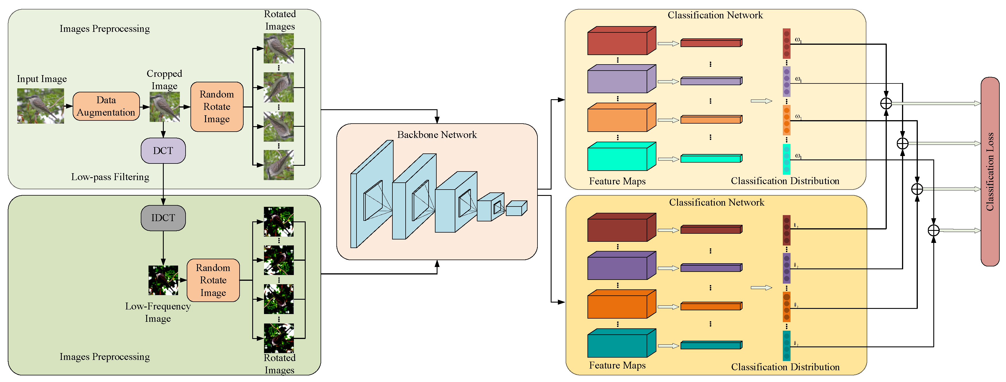
Figure 2.
Examples of the FOAGDDs at a corner and an edge point and the SOAGDDs at a blob at the same location with a lighting change. (a) An original image. (b)-(d) The FOAGDDs of the corner and the edge and the SOAGDDs of the blob on the original image. (e) The original image undergoes a lighting change. (f)-(h) The FOAGDDs of the corner and the edge and the SOAGDDs of the blob on the lighting changed image.
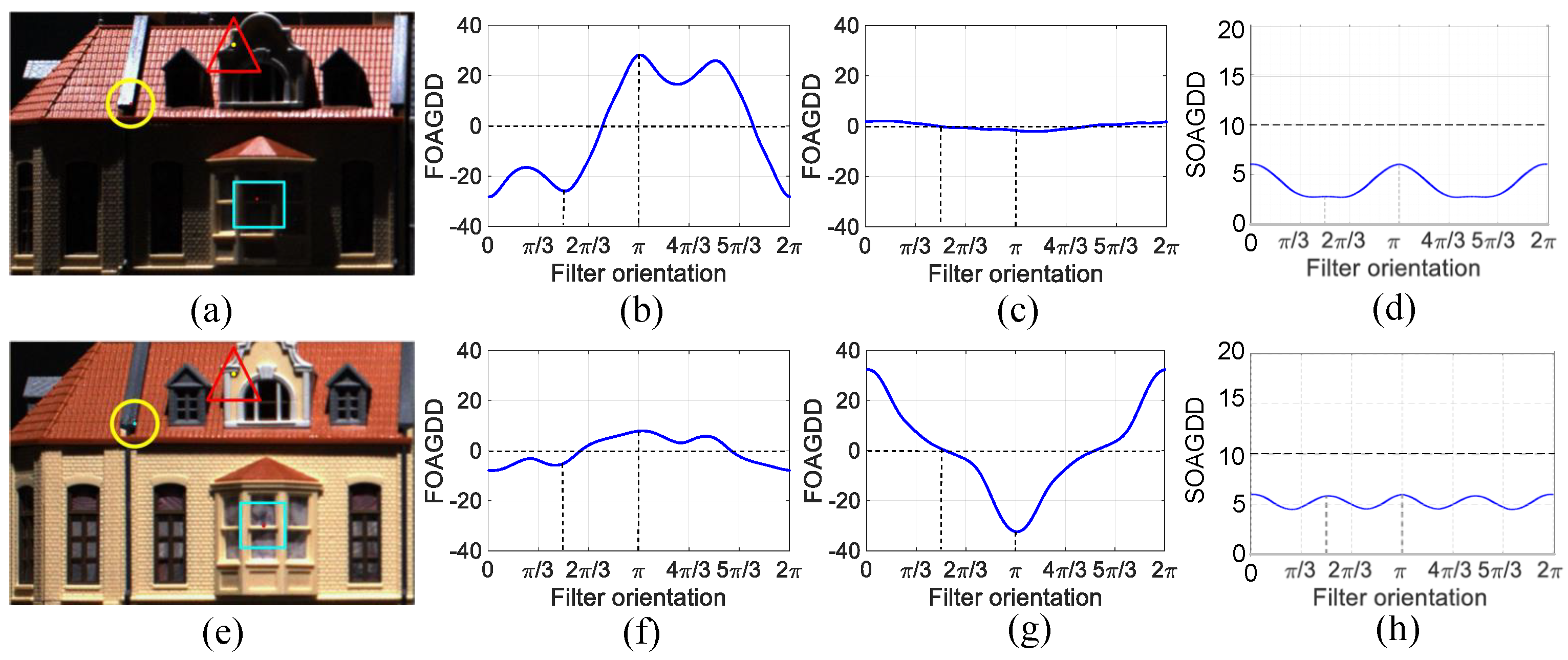
Figure 3.
Examples of the FOAGDDs at a corner and an edge point and the SOAGDDs at a blob at the same location under image affine transformation. (a) An original image. (b)-(d) The FOAGDDs of the corner and the edge and the SOAGDDs of the blob on the original image. (e) The original image undergoes image affine transformation. (f)-(h) The FOAGDDs of the corner and the edge and the SOAGDDs of the blob on the deformed image.
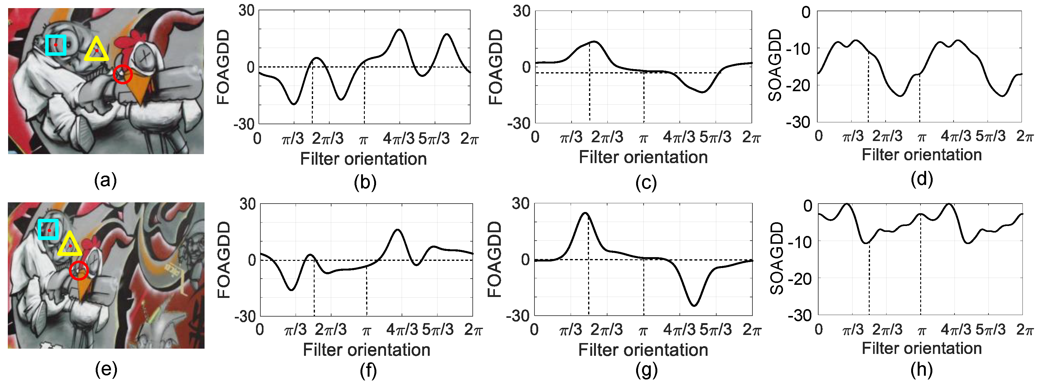
Figure 4.
Examples of LSI-SFD extraction. (a) LSI extraction of existing image data augmentation techniques. (b) LSI-SFD extraction of our proposed information preprocessing.
Figure 4.
Examples of LSI-SFD extraction. (a) LSI extraction of existing image data augmentation techniques. (b) LSI-SFD extraction of our proposed information preprocessing.
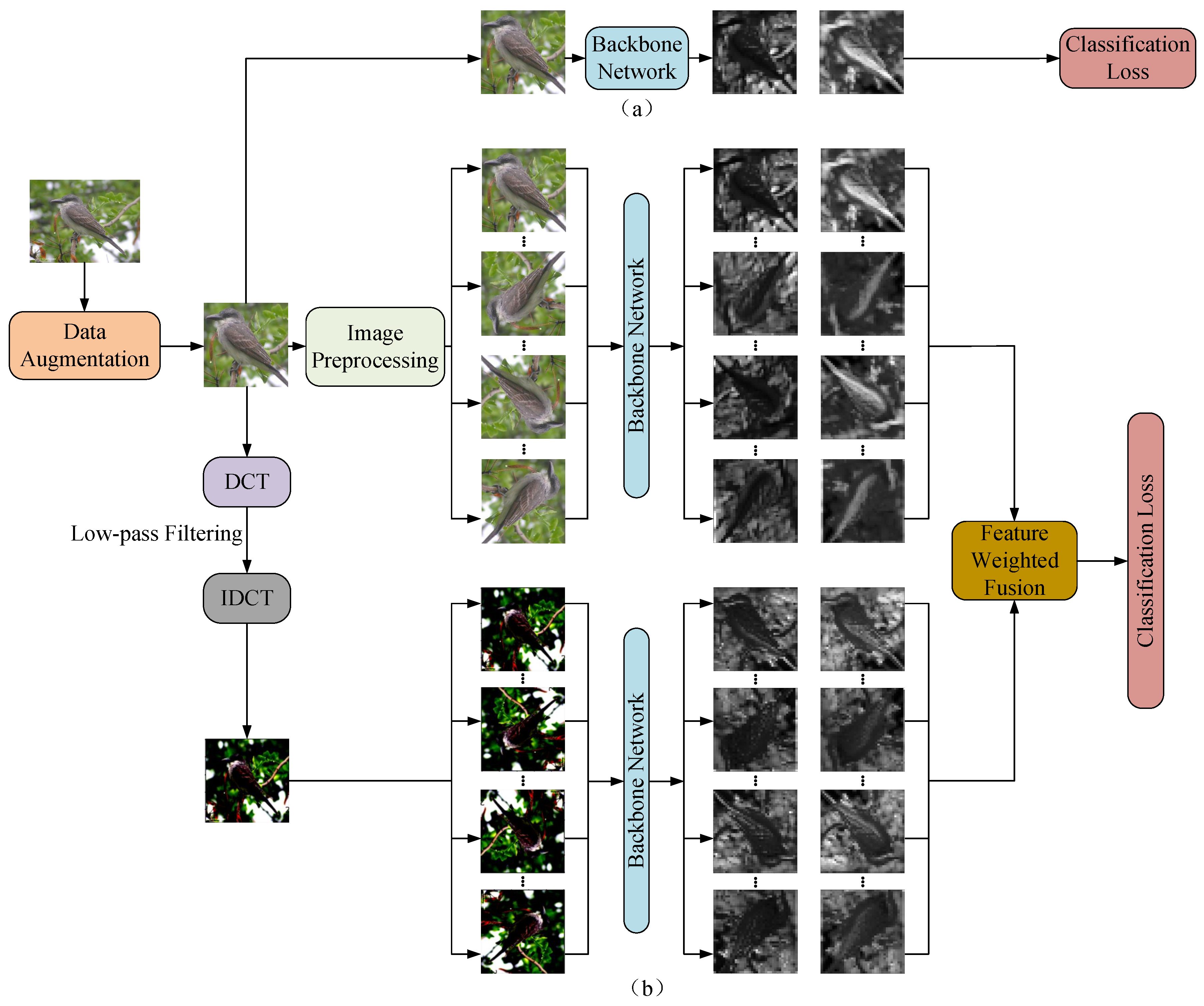
Figure 5.
The impact of different input image sets on SDFGVC performance.
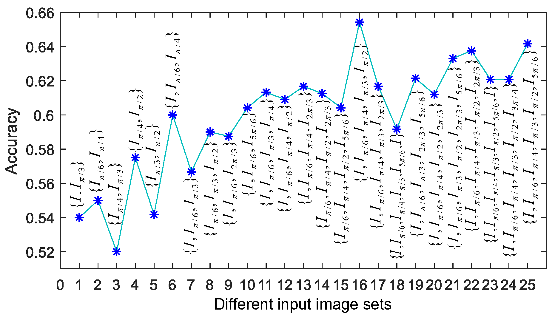
Figure 6.
The impact of the number of epochs for the accuracy of SDFGVC.
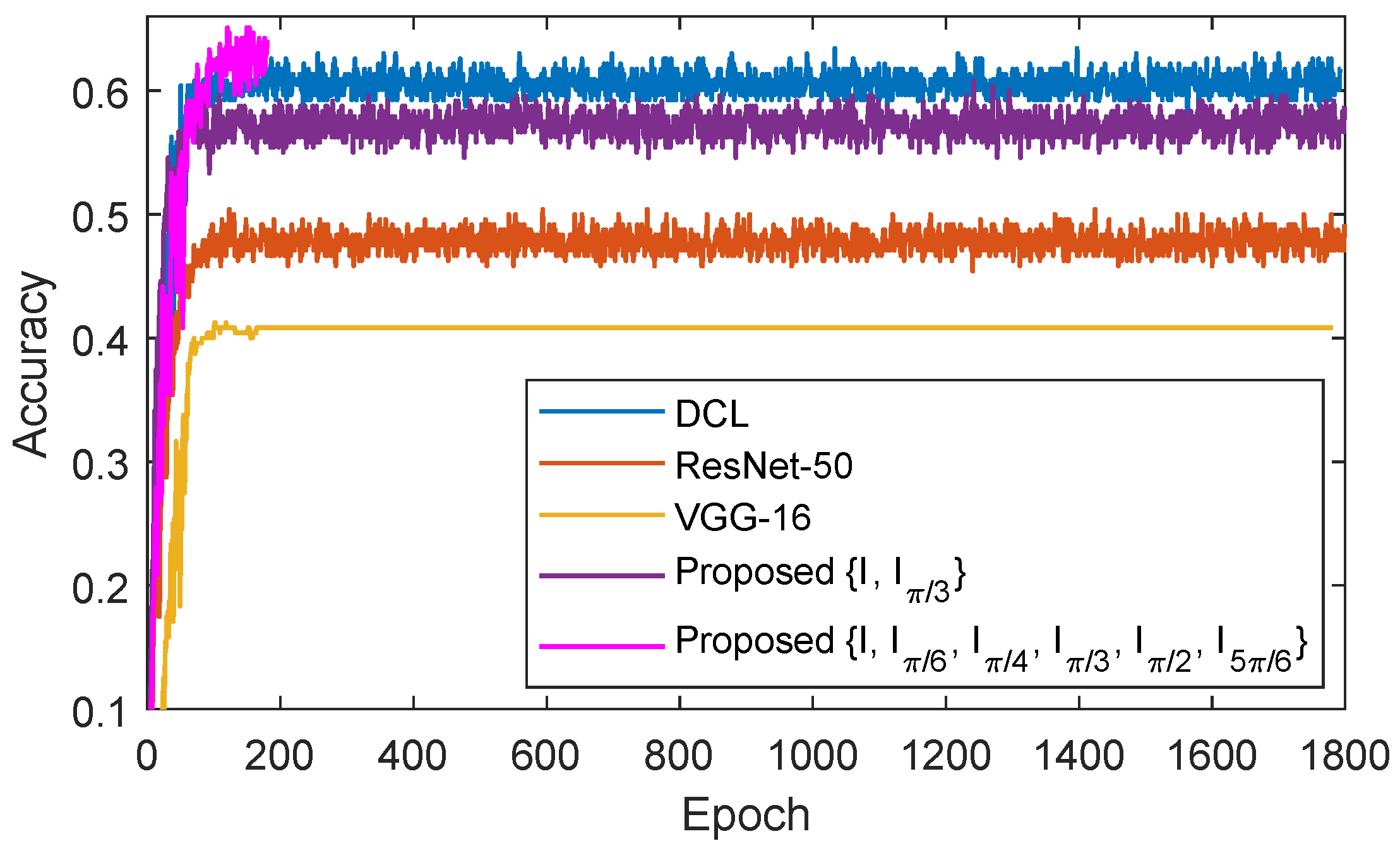
Figure 7.
Using the SAR geographical information image of Zhongchi Town in 2021 for permanent farmland change detection, with GIS Image as the mask image of the standard farmland in 2017. The image of Zhongchi Town uses the 2021 image as the detected image; p1 and p2 are the information of each regular geographical patch segmented from the Zhongchi Town image in 2021 through the mask image.
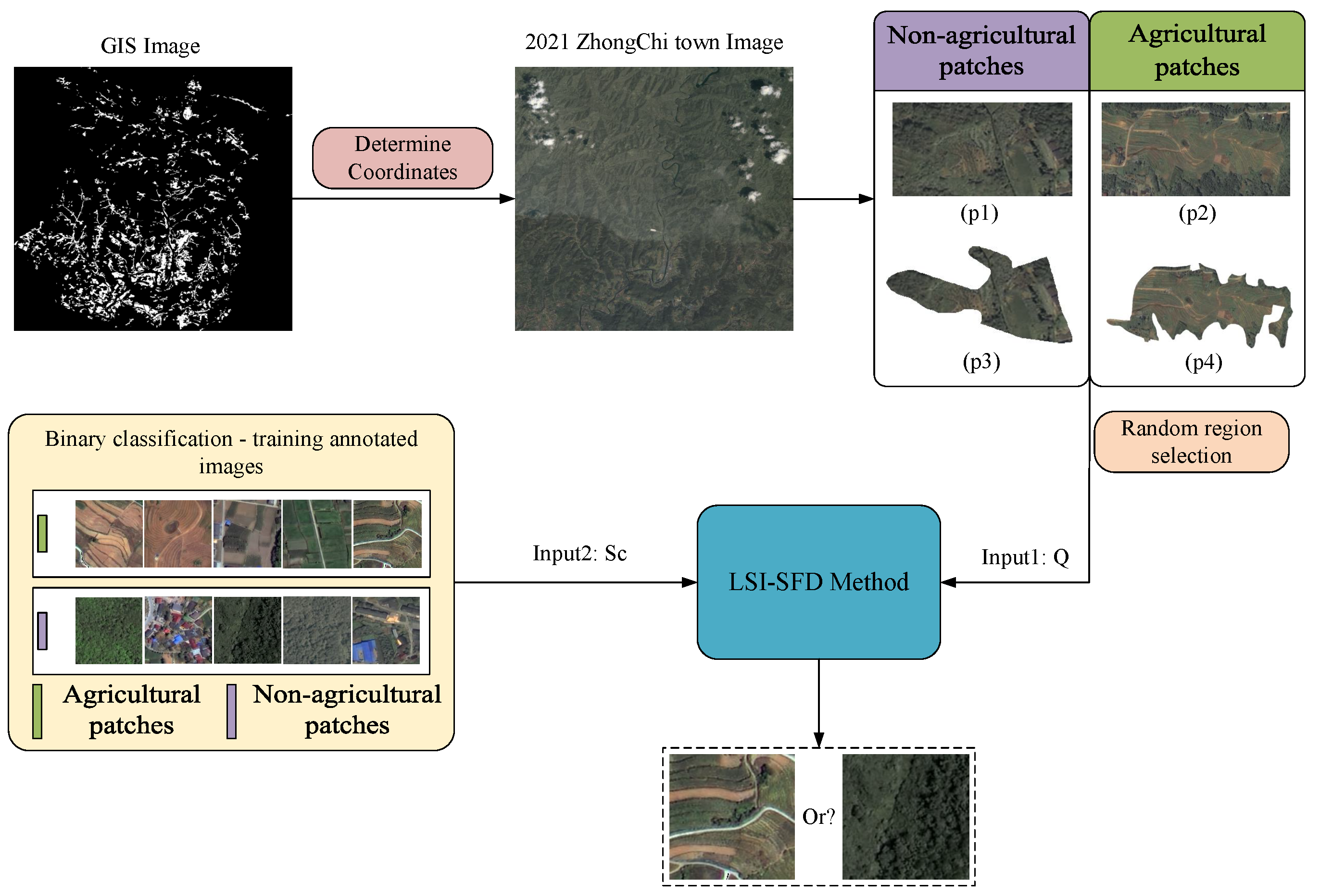

Table 1.
The accuracy of the proposed method with combining six different image rotation directions.
Table 1.
The accuracy of the proposed method with combining six different image rotation directions.
| Input images | Accuracy (%) | |||||
|---|---|---|---|---|---|---|
| Cotton | CUB | CAR | AIR | FLO | PD | |
| 64.89 | 86.63 | 92.77 | 91.07 | 95.49 | 97.46 | |
| 65.33 | 86.63 | 92.32 | 91.23 | 96.16 | 96.58 | |
| 65.42 | 85.29 | 92.89 | 90.79 | 95.49 | 98.72 | |
| 64.37 | 85.13 | 92.26 | 90.47 | 97.18 | 96.46 | |
| 64.63 | 86.16 | 92.13 | 91.43 | 96.84 | 97.58 | |
Table 2.
Comparison with the state-of-the-art methods on six different small datasets with and .
| Method | Base Model | Accuracy (%) | |||||
|---|---|---|---|---|---|---|---|
| Cotton | CUB | CAR | AIR | FLO | PD | ||
| ResNet-50 | Resnet-50 | 48.24 | 84.20 | 90.92 | 89.74 | 95.35 | 96.33 |
| VGG-16 | VGG-16 | 40.19 | 82.18 | 87.55 | 96.32 | 94.37 | 95.17 |
| NTS-Net | ResNet-50 | 52.50 | 84.23 | 90.32 | 88.15 | 95.42 | 96.00 |
| fast-MPN-Cov | ResNet-50 | 50.73 | 85.12 | 88.61 | 90.26 | 96.33 | 95.78 |
| DCL | ResNet-50 | 60.08 | 85.47 | 92.18 | 90.58 | 96.49 | 96.19 |
| Cross-X | ResNet-50 | 52.71 | 85.22 | 92.18 | 89.84 | 96.12 | 93.63 |
| MOMN | ResNet-50 | 40.00 | 81.79 | 86.25 | 85.33 | 97.15 | 98.26 |
| ACNet | ResNet-50 | 53.42 | 85.31 | 92.29 | 88.65 | 96.88 | 96.68 |
| FVD | ResNet-50 | 57.69 | 84.20 | 91.06 | 88.52 | 96.62 | 95.43 |
| Ours | ResNet-50 | 65.42 | 86.63 | 92.89 | 91.43 | 97.18 | 98.72 |
Table 3.
Comparison with the state-of-the-art methods on six different small datasets with and .
| Method | Base Model | Accuracy (%) | |||||
|---|---|---|---|---|---|---|---|
| Cotton | CUB | CAR | AIR | FLO | PD | ||
| ResNet-50 | Resnet-50 | 57.92 | 88.23 | 95.02 | 94.03 | 96.13 | 97.14 |
| VGG-16 | VGG-16 | 48.94 | 85.36 | 90.25 | 95.13 | 95.33 | 96.23 |
| NTS-Net | ResNet-50 | 61.25 | 88.42 | 94.73 | 93.31 | 96.22 | 96.74 |
| fast-MPN-Cov | ResNet-50 | 59.72 | 89.01 | 91.33 | 94.41 | 96.88 | 96.71 |
| DCL | ResNet-50 | 69.91 | 89.92 | 96.17 | 94.53 | 97.09 | 96.97 |
| Cross-X | ResNet-50 | 61.77 | 89.22 | 96.14 | 94.10 | 96.73 | 94.88 |
| MOMN | ResNet-50 | 49.49 | 86.02 | 89.85 | 89.49 | 97.35 | 98.47 |
| ACNet | ResNet-50 | 61.49 | 89.13 | 96.22 | 93.47 | 97.10 | 97.27 |
| FVD | ResNet-50 | 65.91 | 88.95 | 95.36 | 93.77 | 97.01 | 96.53 |
| Ours | ResNet-50 | 74.15 | 90.05 | 96.77 | 95.53 | 97.49 | 98.88 |
Table 4.
Comparison with the existing data augmentation techniques on six different small datasets with and .
Table 4.
Comparison with the existing data augmentation techniques on six different small datasets with and .
| Method | Base Model | Accuracy (%) | |||||
|---|---|---|---|---|---|---|---|
| Cotton | CUB | CAR | AIR | FLO | PD | ||
| Lighting Changes | ResNet-50 | 44.35 | 88.34 | 90.14 | 91.92 | 94.18 | 92.11 |
| Colorizing Images | ResNet-50 | 43.52 | 86.32 | 89.36 | 90.11 | 93.92 | 92.16 |
| Image Rotations | ResNet-50 | 44.24 | 85.66 | 90.12 | 91.37 | 93.15 | 92.21 |
| Image Flips | ResNet-50 | 43.17 | 84.39 | 90.19 | 90.38 | 92.17 | 91.32 |
| Image Affine Transformations | ResNet-50 | 46.78 | 89.91 | 94.36 | 92.18 | 93.96 | 94.49 |
| Ours | ResNet-50 | 74.15 | 90.05 | 96.77 | 95.53 | 97.49 | 98.88 |
Table 5.
The classification accuracy of three algorithms embedded in our proposed framework with and .
Table 5.
The classification accuracy of three algorithms embedded in our proposed framework with and .
| Method | Accuracy (%) | Performance improvement | ||
|---|---|---|---|---|
| Cotton | CUB | Cotton | CUB | |
| Original NTS-Net | 52.50 | 84.23 | 11.71% | 8.45% |
| NTS-Net in our framework | 58.65 | 91.36 | ||
| Original fast-MPN-Cov | 50.73 | 85.12 | 13.97% | 9.38% |
| fast-MPN-Cov in our framework | 57.82 | 93.11 | ||
| Original DCL | 60.08 | 85.47 | 12.21% | 8.14% |
| DCL in our framework | 67.42 | 92.34 | ||
Table 6.
The comparison of change detection accuracy in Zhongchi Town in 2021 with existing methods, with an image size of .
Table 6.
The comparison of change detection accuracy in Zhongchi Town in 2021 with existing methods, with an image size of .
| Method | Base Model | Correct Prediction | Agricultural | Non-Agricultural | Accuracy |
|---|---|---|---|---|---|
| NTS-Net | ResNet-50 | 618 | 37 | 581 | 34.85% |
| fast-MPN-Cov | ResNet-50 | 479 | 16 | 463 | 27.01% |
| DCL | ResNet-50 | 1317 | 116 | 1201 | 74.28% |
| Cross-X | ResNet-50 | 1139 | 97 | 1042 | 64.24% |
| MOMN | ResNet-50 | 1263 | 132 | 1131 | 71.23% |
| Ours | ResNet-50 | 1443 | 189 | 1254 | 80.14% |
Disclaimer/Publisher’s Note: The statements, opinions and data contained in all publications are solely those of the individual author(s) and contributor(s) and not of MDPI and/or the editor(s). MDPI and/or the editor(s) disclaim responsibility for any injury to people or property resulting from any ideas, methods, instructions or products referred to in the content. |
© 2024 by the authors. Licensee MDPI, Basel, Switzerland. This article is an open access article distributed under the terms and conditions of the Creative Commons Attribution (CC BY) license (http://creativecommons.org/licenses/by/4.0/).
Copyright: This open access article is published under a Creative Commons CC BY 4.0 license, which permit the free download, distribution, and reuse, provided that the author and preprint are cited in any reuse.


