
Submitted:
19 September 2023
Posted:
21 September 2023
You are already at the latest version
Abstract
Abstract:The objects of fine-grained image categories(e.g., bird species) are various subclass under different categories. Because the differences between subclass are very subtle and most of them are concentrated in multiple local areas, the task of fine-grained image recognition is very challenging. At the same time, some fine-grained networks tend to focus on a certain region when judging the target category, resulting in the lack of other auxiliary regional features. To this end, Inception V3 is used as the backbone network, and an enhanced and complementary fine-grained image classification network is designed. While adopting the method of reinforcement learning to obtain more detailed fine grain image features, the complementary network can obtain the complementary discriminant area of the target through the method of attention erasure to increase the network's perception of the overall target. Finally, experiments are conducted on CUB-200-2011, FGVC Aircraft and Stanford dogs three open datasets. The experimental results show that the proposed model has better performance.
Keywords:
fine grain image recognition
; Inception-V3
; reinforcement complementary learning
; complementary learning
; inter-class gap
1. Introduction
Fine-grained image classification, that is, identifying the subclass of different kinds of objects, is a hot research topic in the fields of image recognition, computer vision and other fields in recent years. Compared with traditional image classification tasks, its research content is mainly to identify different subclass under a certain category. For example, the detailed classification of different types of vehicles in urban management can be used as the basis for traffic detection and tracking reference, and the identification of different types of goods can help businesses analyze consumer buying habits and adjust sales strategies. Similar to other computer vision tasks, fine-grained image classification methods have many common problems, such as uneven illumination, large scene differences, and variable scales and perspectives. At the same time, the biggest challenge of fine-grained image classification comes from its characteristics of small inter-class differences and large intra-class differences. Therefore, how to find highly recognizable object components from these fine-grained images is a difficult problem to be solved in the current fine-grained recognition field. Some methods use additional manual labeling information [1,2,3,4] (such as bird's head, tail and other areas) to help the convolution neural network locate local areas with high distinguishability. Although these methods have achieved good results, they require a lot of manpower. Another kind of method uses weak supervision to locate local areas, and needs image label information in the experiment process. Fu et al. [5] proposed the RACNN model to identify by region detection and fine grain feature mutual reinforcement. This method can well locate the most discriminative local areas, but the increasing scale will lead to the loss of secondary features. Zheng et al. Therefore, in this paper, Inception-V3 is used as the feature extraction network, and a fine-grained image classification network based on reinforcement complementary learning is designed. The network can obtain more detailed fine-grained features of the target through reinforcement learning strategy. In order to deal with the multi-pose and multi-angle problems commonly existing in the target, the model is forced to learn other complementary discriminative regions through complementary learning strategy, Finally, the obtained features are spliced to improve the overall recognition effect of the network for the target.
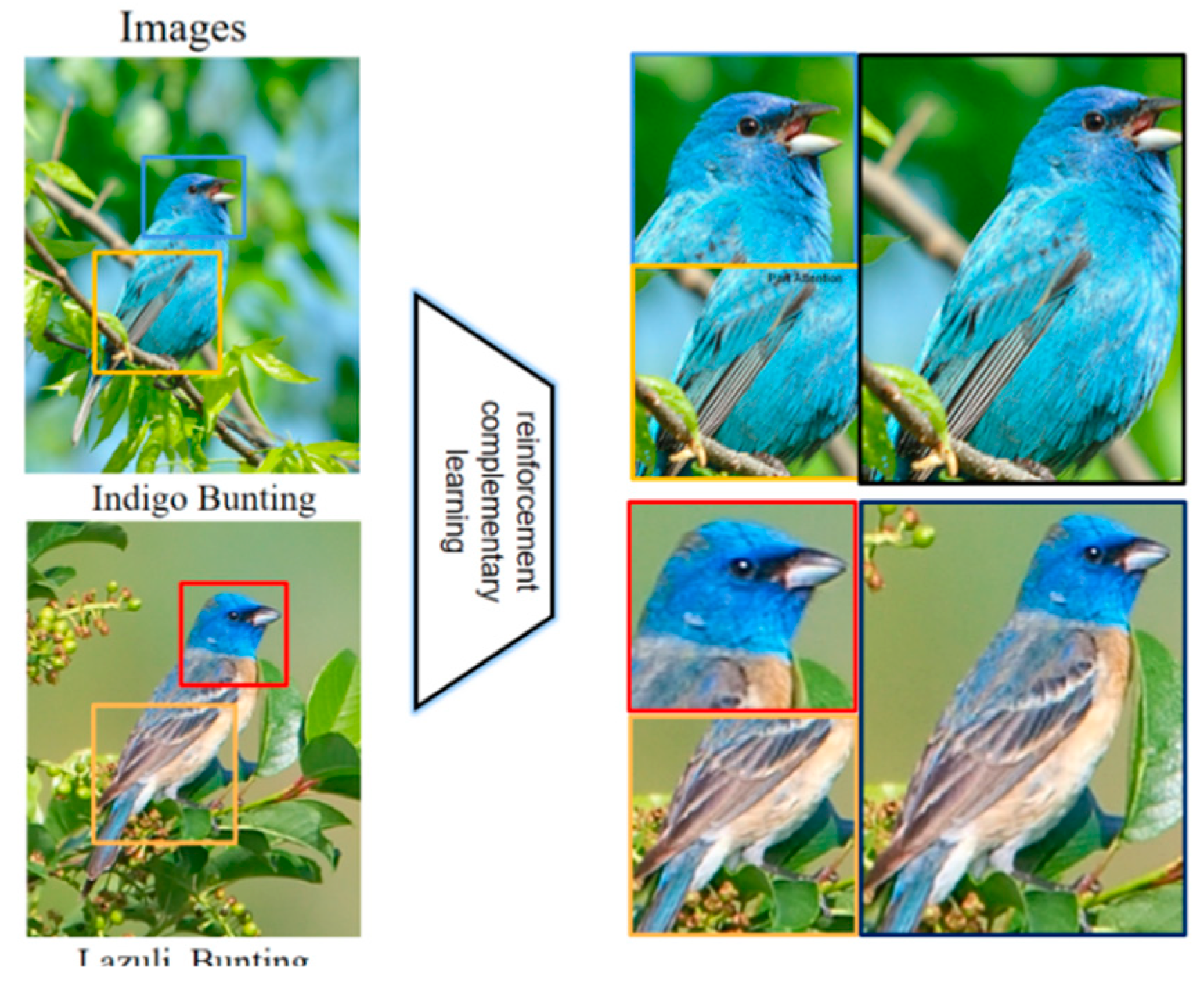
Figure 1.
Strengthen complementary learning strategies.
2. Related work
The method of strong supervision requires a lot of manual annotation to obtain important local information. However, with the increasing amount of data, manual annotation is obviously inappropriate. At present, for fine-grained recognition tasks, the common approach is to use weak supervision to make the model automatically focus on the salient regions and extract features. To this end, we will focus on the way of weak supervision:
(1) The method based on local location. In local localization, the method of constructing local localization subnetwork is relatively common. Literature [6,7,8] uses semantic component localization subnetwork to locate the key area of fine-grained image and then learn. In addition, it is also possible to learn fine-grained features through segmentation of semantic components. Huang et al[9] established an interpretable model with high accuracy by combining prior knowledge and regional parts. The interpretation of the model is carried out through segmentation of semantic components and their contribution to classification. Different from the above methods, Ge et al [10] established a complementary part model, and extracted the semantic parts of fine-grained objects by using the segmentation of Mask R-CNN and CRF, so that the model can focus on the most discriminating secondary parts.
(2) End-to-end feature coding method. Second-order bilinear features have good feature representation ability. Lin et al. proposed BCNN [11], which extracts features through two parallel convolution neural networks and then multiplies them by outer product. However, the feature dimension generated by this method is very large, which is not conducive to model training. Taking ResNet-50 as an example, the resulting dimension is as high as 2048 * 2048. In order to reduce the dimension, the original bilinear feature is approximated by compressing bilinear feature [12], bilinear pooling [13] and Hadamard product [14], and the parameter quantity is compressed by more than 90%; Dubey A et al. [15] introduced confusion in activation to reduce over-configuration, and used Pairwise Fusion regularization to reduce over-fitting.
(3) Methods based on attention mechanism. Zheng et al[16] TASN method, which uses the trilinear attention module to model the relationship between channels to generate an attention graph, and uses the content represented by the graph to learn features; Liu[17] proposed that Full Convolutional Attention Localization Networks. The structure of FCANs is mainly composed of three parts: feature extraction, full convolution local area attention network, and classification network. Among them, the full convolution network locates multiple key areas of the image, and uses convolution features to generate fractional mapping for each part, and finally obtains the classification results; Zheng et al[18] proposed MACNN, which is composed of convolution, channel grouping and local classification. The convolution feature based on the region is extracted from the input image through convolution layer. The peak response region feature of the feature map is used to cluster the channels with similar response regions to obtain local regions with discrimination. At the same time, the channel grouping loss function is used to increase the inter-class differentiation and reduce the intra-class differentiation; Zhang et al[19] control the contribution of different regions to recognition through the gating mechanism; Zhu et al[20] proposed a simple and effective cross door attention learning strategy that guides the final classification through rich discriminative features in key regions, and achieved good results.
3. RACL-NET(Reinforcement And Complementary Learning network)
3.1. The network structure
For a recognition network, the features it pays attention to tend to focus on a certain area of the target, which becomes the most important feature for identifying the target. However, we hope that the designed model can identify the target in a larger range, which can be achieved by relying on secondary features as well as no longer relying on a certain salient feature,it mainly uses data occlusion to achieve target recognition on a larger scale[21].So this paper designs a complementary learning reinforcement network model, which drives the other two sub-networks to carry out reinforcement learning and complementary learning(This is a kind of adversarial learning. Two parallel classifiers are forced to use complementary target regions for classification, and finally generate complete target localization together) respectively through the feature extraction of the backbone network, so as to realize the detailed and comprehensive recognition of the recognition target. Its network structure is shown below:
Figure 2.
The structure of RC-Net.

The network structure is composed of Inception V3, which are the basic network, the reinforcement network and the complementary network. By building a three-way classification network to aggregate the overall and local features of the object, we can obtain both the overall semantic information of the object and the local semantic information of the object. Then we can pool the global average of the features output from each network, three 2048 dimensional eigenvectors can be obtained and then splice the pooled features to form a 6144 dimensional eigenvector, Add a 200-dimensional classification layer to the vector for end-to-end training, and finally get the classification results through Softmax.
3.2. Drive model
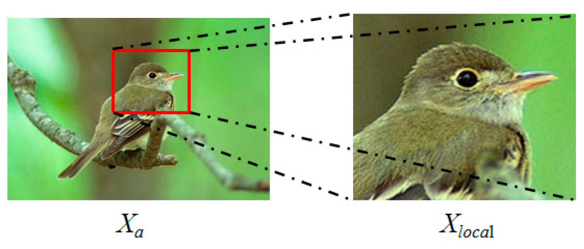
Traditional neural networks do not take advantage of the advantages of deep neural networks for location and recognition learning. Inspired by the attention region recommendation network APN, this paper proposes a module DM (Drive Model) that can drive complementary learning and reinforcement learning. DM is a very important structure in this model. It can help the backbone network find the rectangular region that has the greatest impact on the results during the training process. Specifically, It has two functions: on the one hand, it cuts and enlarges the area that has the greatest impact on the result and sends it into the reinforcement network; on the other hand, it erases the rectangular area in the original image and sends it into the complementary network. At the same time, the calculation cost of DM module is very small, and it can help the model to conduct end-to-end training.
DM receives the characteristic map of the basic network after training, and then it will generate a square area with as the center and half of as the side length, and cut and enlarge the area and send it into the reinforcement network. At the same time, it will also generate an image mask based on the area and input it into the complementary network for complementary learning.
In this process, the high response area of the feature map is the key to obtain the coordinate . The DM module is composed of two full connection layers. The network input is the feature map, and the output is the coordinates of the boundary box of the high response area. The automatic location of the most important local area can be achieved through the full connection layer. Therefore, we have limited the size of the bounding box, which can not exceed 2/3 of the longest edge of the overall image at most and 1/3 of the smallest edge of the image at least.
Specifically, given an image X, input it into the trained convolution layer for feature extraction, represents the overall parameters, and the whole process can be described as convolution, pooling, activation, and finally generating a probability distribution p, with the following calculation formula:
In this formula, represents the full connection layer, which converts the features extracted by the convolution neural network into feature vectors, and uses Softmax to convert this vector into probability values. The next step is to generate the position and length parameter information of the square bounding box, specifically:
Where is half of the horizontal and vertical coordinates and side length of the bounding box in X, represents the DM module, and its structure is composed of two fully connected layers. The weight parameters of network initialization have a great impact on the model, so the output characteristic graph of the last layer of the basic network is added. This is because the later the number of layers of the neural network is, the richer the semantic information of the characteristic graph is, and the more accurate the generated bounding box is. The region with the largest value can be obtained by adding the feature map, which is the most critical area in the image, and the parameter information of the region is the initialization parameter of the DM module. The specific formula is:
Where, f represents the feature map output at the last layer of the convolutional neural network, n represents the feature map’s number, d represents the total number of feature maps, F represents the total feature map after adding each feature map. And then compares the F and . If F is greater than , then F is 1, otherwise F is 0, as shown in formula 5. Select the side length of the largest area as the side length of the bounding box, and the implementation formula is:
In (4), h and w represent the width and height of the feature map, and represents the mean value of the feature map. By comparing the size of and , the initialization coordinates of the bounding box center are generated. After obtaining the initial coordinates, the model can automatically optimize the coordinates according to the training process, and then the region needs to be trimmed and enlarged to obtain a more detailed local region and then sent to the reinforcement network for learning. The coordinates of the upper left corner and the lower right corner of the local area are obtained according to the center coordinate and side length. The coordinates of the upper left corner are recorded as , and the coordinates of the lower right corner are recorded as . The calculation process is as follows:
After obtaining the coordinate information, the clipping operation can be seen as the multiplication between the original image I and the template, expressed as:
In this formula, is the clipped area, is the clipping operation between the original image and the template, is the attention mask, and its expression is:
In this formula, i and j are at any point in the feature map. If i and j are located inside the feature map, the value of is 1, otherwise the value is 0. At the same time, is a continuous differentiable function, whose expression is:
In addition, in order to cut and enlarge the image, the bilinear interpolation method is used to expand the size of the extracted local area. According to the ratio of the original image and the local area, the enlarged local area can be obtained. The formula is as follows:
and represent the area of the local area and the overall area, is the area ratio, is the enlarged local area. Strengthen training on key areas of the image according to .
Figure 3.
Local area amplification.
In order to train the complementary network, the generated local area is changed into a mask image. The mask pixels are uniformly the mean value of the original image pixels, and the rest are replaced by white pixels, as shown in the following formula:
After that, the mask is erased from the original image according to the previously obtained position information, and the obtained mask image is sent to the complementary model training. The specific process is as follows
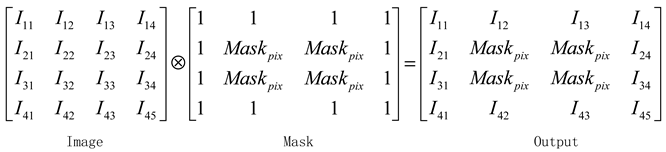
In this formula, the values of each position in the pixel matrix formed by the original image represent different pixels, 1 in the mask image represents black pixels, and the pixel values in the RGB channel are (0, 0, 0). Through the position calculation of the original image and the mask, the black pixel part is directly filled with the original pixel, and the mask pixel will replace the original pixel, which can also obtain the image after erasing the key area. As shown in Figure 4:
3.3. Loss function
The loss function has a great impact on the model, and the appropriate loss function has a positive impact on the model training. The commonly used loss function for fine-grained image recognition is the softmax loss function, and the formula is shown :
Where, m represents the size of a batch, W represents the output result of the full connection layer, represents the category of the image, represents the feature vector of the image before the full connection layer, b represents the network offset, and s represents the number of target categories.
The Softmax is used to optimize the classification network. In order to enable the DM model to locate the key areas, the loss function of DM is designed. It is used to continuously optimize and strengthen the location information of the network, and at the same time, it provides more accurate mask location to enable the complementary network to learn secondary features.
In this formula, represents the probability value of the output sample of the backbone model, while represents the probability value generated by the reinforcement model. Here, the value of p is obtained according to formula 1, the represents the difference between the two models, which is 0.05. When >, there is no loss; when <, there is loss. Therefore, the loss function can help the reinforcement network to find more accurate features, and after extracting accurate features, it can help the backbone network to locate more accurately. The two strengthen each other.
At the same time, in the complementary model, because the features extracted from the backbone feature will be erased, the features extracted from the backbone model have no connection with the complementary model at all. However, the precise local area provided by the backbone model is conducive to the secondary feature learning of the complementary model, so it is only necessary to ensure that the backbone model and the reinforcement model can locate the key parts. From the above example, the total loss of the model is:
Where is the modulation coefficient, which is used to balance the two loss functions.
4. Experiments and Discussions
4.1. Datasets
Datasets: In order to verify the performance of this model, three challenging fine-grained public data sets are compared, including CUB-200-2011, Stanford Cars, and FGVC-Aircraft.
(1) CUB-200-2011: The data set includes 200 different types of birds, including 5994 images in the training set and 5794 images in the test set, a total of 11788 images.
(2) Stanford Cars: The data set includes 196 types of vehicles of different brands and years, including 8144 images in the training set and 8041 images in the test set, a total of 16185 images.
(3) FGVC-Aircraft: The data set includes 100 different types of aircraft, including 6667 images in the training set and 3333 images in the test set, totaling 10000 images.
4.2. Erase experiment
The purpose of designing the complementary network is to improve the ability of the model to pay attention to secondary features, which is very important for strengthening the complementary learning network. However, we also note that different data must have different feature distributions, which will affect the experimental results. A small number of data may need to be erased in key areas several times to obtain all features. In the AE-PSL[22] model, the experimenter erased the original image twice to obtain the overall characteristics of the target. Therefore, in this paper, it is necessary to conduct erasure experiments on the data set used to find the appropriate erasure times.
From the above Figure 5, after using CAM[23] to visualize the original image, the feature extraction network only focuses on the most important local area. Erasing this area, we can find that the focus of the feature extraction network is shifted to the secondary part. If the secondary part is erased again, the network cannot find the effective local area, so the best erasing number is 1, which is the same as the erasing number of the complementary model in this paper.
4.3. Experimental steps
The method proposed in this paper mainly consists of three steps, which are to train the backbone model using the transfer learning method, and then train the reinforcement network and the complementary network in turn according to the training results of the feature extraction network until the three networks converge.
1) Migration learning is a very common way of training neural networks at present. It uses the training weight of Perception V3 on Image Net to train the feature extraction network. The parameters of pooling layer, input layer and convolution layer are reserved. The existing full connection layer and Softmax layer are removed to fine-tune the network and train the data used in this paper.
2) The training of the reinforcement network is carried out according to the results of the feature extraction network. Through the calculation of the key area by the feature extraction network, the coordinate information of the most critical area is found to be cut and amplified to produce more detailed training results. The training principle of the complementary network is similar to that of the reinforcement model. The coordinate information generated by the feature extraction network is erased, and the image with only secondary local area is generated to strengthen the ability of the model to pay attention to secondary features.
4.4. Parameter setting
The experimental environment is carried out under the version of Pythoch1.71. The GPU is Nvidia Genforce 3060Ti, and the CPU is i7-10700K. The optimizer selects SGD, the initial learning rate is set to 0.0001, the momentum super-parameter is 0.9, batch_ Size is 32, and epoch is set to 200.
4.5. Visualization of experimental results
In order to prove that the proposed reinforcement complementary learning network can better capture the characteristics of other auxiliary discriminant regions, this paper uses CAM algorithm to activate the class diagram of a single reinforcement network and reinforcement complementary network. The experimental results are shown in the following Figure 6
In Figure 6, (a) represents the attention heat map after using only feature extraction network Inception V3. It can be found that the network focuses on the most important area of the target, and the range of the heat map is small. (b) It indicates the target area that the network pays attention to after using reinforcement complementary learning. It can be clearly found that the range of red heat map becomes larger and more local areas are concerned.
4.6. Experimental verification and analysis
4.6.1. Ablation experiment
In order to further verify that the various network structures proposed in this paper can effectively improve the network performance, three sets of comparative tests have been conducted on CUB-200-2011. The experimental settings and results are shown in Table 1:
4.6.2. Comparison test
In order to verify the superiority of the algorithm in this paper, experiments were carried out on three open fine-grained image data sets CUB-200-2011, FGVC-Aircraft, and Standard-dogs, and the accuracy reached 89.5%, 93.6%, and 94.8%, and some of the latest models were selected for comparison, as shown in the following table:

Table 2.
Accuracy of related methods in CUB_200_2011.
| Method | Top-1 Acc(%) |
|---|---|
| B-CNN[11] | 84.1 |
| MA-CNN[6] | 86.5 |
| DFL-CNN[24] | 87.4 |
| DCL[25] | 87.8 |
| SPS[32] | 88.7 |
| DB[26] | 88.6 |
| DCAL[33] | 88.7 |
| FDL[27] | 89.0 |
| RACL-Net | 89.5 |
5. Conclusions
We propose a reinforcement complementary learning network to classify fine-grained images. The work done in this paper shows that the reinforcement model can help the network to obtain more detailed local features. At the same time, for the multi-pose and multi-angle problems commonly existing in fine-grained images, obtaining other complementary discriminant regions through the reinforcement model can also improve the effect of fine-grained image recognition. Finally, our reinforcement complementary learning network is weakly supervised, and it can be widely used in other classification tasks.In the future, we will explore more efficient fine-grained image classification methods, which will be carried out from the following two aspects: first, how to fuse more local regions to judge the fine-grained image classification to improve the model recognition effect; Secondly, how to build interpretable models of complementary regions to continuously improve the model recognition effect on a more detailed scale.
References
- ZHANG N, DONAHUE J, GIRSHICK R, et al. Part-based R-CNNs for fine-grained category detection[M]//ECCV European Conference on Computer Vision (ECCV).2014: 834-849.
- ON S, VAN HORN G, BELONGIE S, et al. Bird species categorization using pose normalized deep convolutional nets[EB/OL].(2014-06-11)[2021-09-15]. https://arxiv.org/abs/1406.2952.
- Lin T Y, ROYCHOWDHURYA, MAJI S. Bilinear CNN Models for Fine-Grained Visual Recognition[C]//ICCV Proceedings of the 15th IEEE International Conference on Computer Vision (IEEE).Santiago,Chile:2015:1449-1457.
- DONAHUE J, JIA Y Q, VINYALS O, et al. DeCAF: A deep convolutional activation feature for generic visual recognition[C]// Proceedings of the 31st International Conference on Machine Learning. New York: JMLR. org,2014:647-655.
- FU J,ZHENG H,TAO M. Look Closer to See Better: Recurrent Attention Convolutional Neural Network for Fine-grained Image Recognition[C]∥IEEE Conference on Computer Vision and Pattern Recognition (CVPR).2017:4438-4446.
- ZHENG H,FU J,TAO M, et al. Learning Multi-attention Convolutional Neural Network for Fine-Grained Image Recognition[C]//ICCV International Conference on Computer Vision (ICCV).2017:5209- 5217.
- SUN M,YUAN Y,ZHOU F, et al. Multi attention multi-class constraint for fine-grained image recognition [C]//ECCV Proceedings of the European Conference on Computer Vision (ECCV).2018:805-821.
- WANG Y,MORARIU V I,DAVIS L S. Learning a discriminative filter bank within a CNN for fine-grained recognition[C]//IEEE Conference on Computer Vision and Pattern Recognition (CVPR).2018 :4148-4157.
- Huang,ZXu, DTao,YZhang. Part-Stacked CNN for Fine-Grained Visual Categorization[C]//IEEE Conference on Computer Vision and Pattern Recognition (CVPR).2016:1173-1182.
- WGe, XLin, YYu. Weakly Supervised Complementary Parts Models forFine-Grained Image Classification From the Bottom Up[C]//IEEE/CVF Conference on Computer Vision and Pattern Recognition (CVPR).2019: 3029-3038.
- Lin T, ROYCHOWDHURY A, MAJI. Bilinear S.CNN Models for Fine-Grained Visual Recognition[C]//IEEE International Conference on Computer Vision (ICCV). 2015:1449-1457.
- SHU K, FOWLKES C. Low-Rank Bilinear Pooling for Fine-Grained Classification[C]//IEEE Conference on Computer Vision and Pattern Recognition (CVPR).2017:365-374.
- GAO Y,BEIJBOM O,ZHANG N,et al. Compact bilinear pooling[C]//IEEE Conference on Computer Vision and Pattern Recognition (CVPR).2016:317-326.
- DUBEY A, GUPTA O, RASKAR R, et al. Maximum entropy fine grained classification[J]. ArXiv Preprint ArXiv,2018:1809.05934.
- GAO Y, EIJBOM O, HANG N, et al. Compact bilinear pooling[C]//2016 IEEE Computer Vision and Pattern Recognition(CVPR).2016:317-326.
- H Zheng,J Fu,Z Zha, et al. Looking for the Devil in the Details: Learning Trilinear Attention Sampling Network for Fine-Grained Image Recognition[C]//2019 IEEE/CVF Conference on Computer Vision and Pattern Recognition (CVPR), 2019:5007-5016.
- LIU X, XIA T, WANG J, et al. Fully convolutional attention networks for fine⁃grained recognition[EB/OL]. (2017-03-21)[2021-11-11]. https://arxiv.org/pdf/1603.06765.pdf.
- ZHENG H L, FU J L, MEI T, et al. Learning multi⁃attention convolutional neural network for fine⁃grained image recognition[C]// Proceedings of the 2017 IEEE International Conference on Computer Vision. Piscataway: IEEE,2017:5219-5227.
- L Zhang,S Huang,W Liu, et al. Learning a Mixture of Granularity-Specific Experts for Fine-Grained Categorization[C]//2019 IEEE/CVF International Conference on Computer Vision (ICCV), 2019: 8330-8339.
- Zhu Q, Kuang W, Li Z. A collaborative gated attention network for fine-grained visual classification[J]. Displays, 2023: 102468. [CrossRef]
- Ning E, Zhang C, Wang C, et al. Pedestrian Re-ID based on feature consistency and contrast enhancement[J]. Displays, 2023: 102467. [CrossRef]
- Wei Y, Feng J, Liang X, et al. Object region mining with adversarial erasing: A simple classification to semantic segmentation approach[C]//Proceedings of the IEEE conference on computer vision and pattern recognition. 2017: 1568-1576.
- Zhou X, Li Y, Cao G, et al. Master-CAM: Multi-scale fusion guided by Master map for high-quality class activation maps[J]. Displays, 2023, 76: 102339. [CrossRef]
- DFL-CNN:Yang Z, Luo TG, Wang D, et al. Learning to navigate for fine-grained classification. Proceedings of the 15th European Conference On Computer Vision. Cham: Springer, 2018. 420–435.
- DCLCHENY,BAIY,ZHANGW,et al.Destruction and Construction Learning for Fine-Grained Image Recognition[C]∥IEEE/ CVF Conference on Computer Vision and Pattern Recognition (CVPR).2019:5152-5161.
- DBSUNG,CHOLAKKALH,KHANS,etal.Fine-Grained Recognition:Accounting for Subtle Differences between Similar Classes[J].Proceedings of the AAAI Conference on Artificial Intelligence,2020,34(1):12047-12054. [CrossRef]
- FDL;LIU C,XIE H,ZHAZJ,etal.Filtration and Distillation:Enhancing Region Attention for Fine-Grained Visual Categorization [C]∥AAAI Conference on Artificial Intelligence.2020: 11555-11562. [CrossRef]
- LUO W, ZHANG H, LI J, et al. learning Semantically Enhanced Feature for Fine-Grained Image Classification[J]//2020 IEEE Signal Processing Letters (IEEE).2020,27:1545-1549. [CrossRef]
- ZHAO B,WU X,FENGJ,etal.Diversified Visual Attention Networks for Fine-Grained Object Classification [J].IEEE Transactionson Multimedia,2017,19(6):1245-1256. [CrossRef]
- DUBEY A,GUPTA O,GUO P,et al.Pairwise Confusion for Fine-Grained Visual Classification[C]∥European Conference on Computer Vision(ECCV).2018:71-88.
- CHEN Y,BAIY,ZHANG W,et al. Destruction and Construction Learning for Fine-Grained Image Recognition[C]∥IEEE/CVF Conference on Computer Vision and Pattern Recognition(CVPR).2019:5152-5161.
- Shaoli Huang, Xinchao Wang, and Dacheng Tao. Stochastic partial swap: Enhanced model generalization and interpretability for fine-grained recognition. In Proceedings of the IEEE/CVF International Conference on Computer Vision, pages 620–629, 2021. 5.
- Zhu H, Ke W, Li D, et al. Dual cross-attention learning for fine-grained visual categorization and object re-identification[C]//Proceedings of the IEEE/CVF Conference on Computer Vision and Pattern Recognition. 2022: 4692-4702.
Figure 4.
Mask generation.
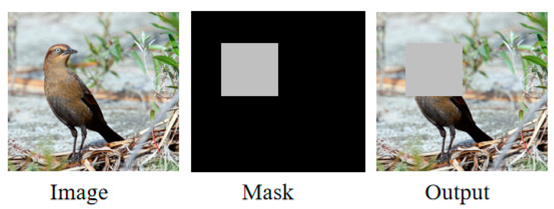
Figure 5.
Erase times experiment.
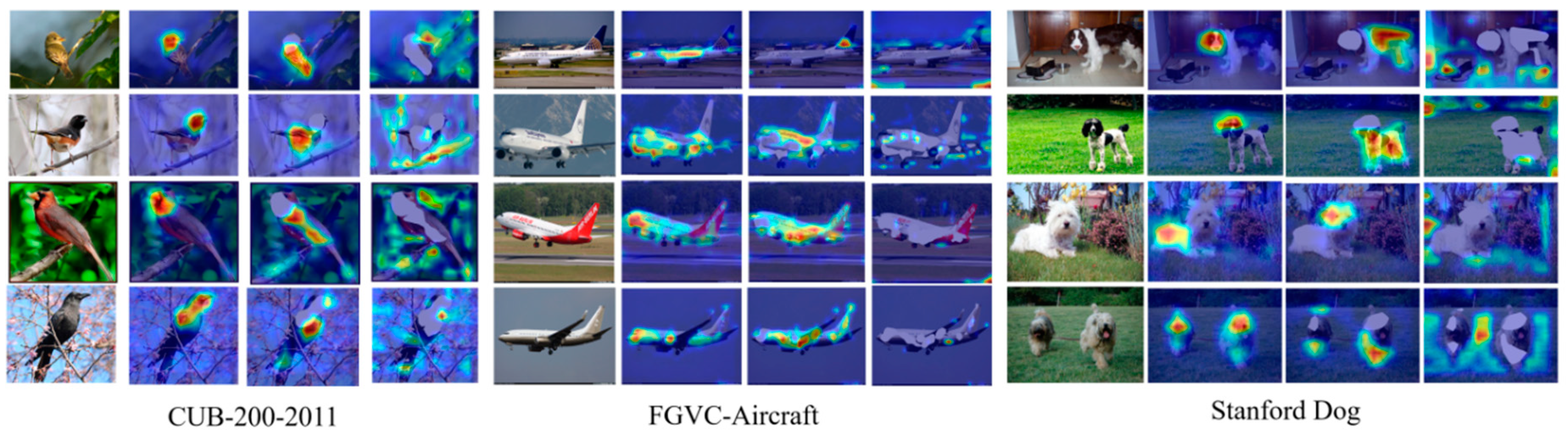
Figure 6.
Visualization of RACL-Net results.
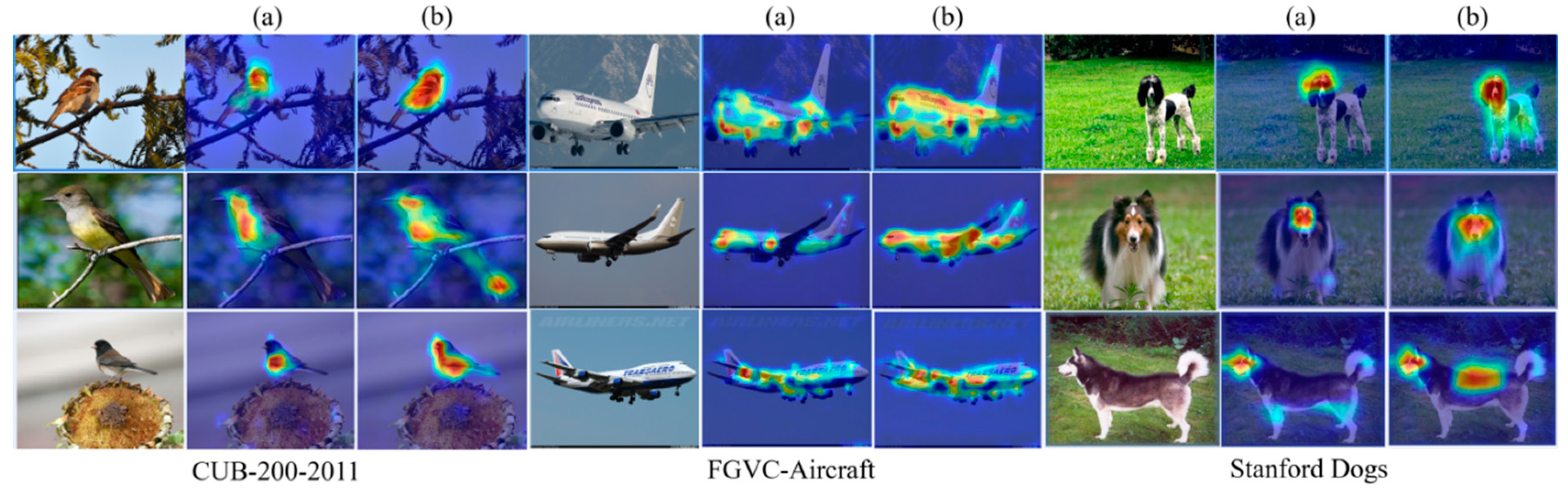
Table 1.
Ablation experiments on the CUB-200-2011 Datasets.
| CUB-200-2011 | Experiment1 | Experiment2 | Experiment3 |
|---|---|---|---|
| Inception-V3 | √ | √ | √ |
| Strengthen network | √ | √ | |
| Complementary network | √ | ||
| Top-1Acc/% | 83.5 | 85.6 | 89.5 |
Disclaimer/Publisher’s Note: The statements, opinions and data contained in all publications are solely those of the individual author(s) and contributor(s) and not of MDPI and/or the editor(s). MDPI and/or the editor(s) disclaim responsibility for any injury to people or property resulting from any ideas, methods, instructions or products referred to in the content. |
© 2023 by the authors. Licensee MDPI, Basel, Switzerland. This article is an open access article distributed under the terms and conditions of the Creative Commons Attribution (CC BY) license (http://creativecommons.org/licenses/by/4.0/).
Copyright: This open access article is published under a Creative Commons CC BY 4.0 license, which permit the free download, distribution, and reuse, provided that the author and preprint are cited in any reuse.


