
Submitted:
11 December 2024
Posted:
12 December 2024
You are already at the latest version
Abstract
Based on the observations of dynamical system, we define partition ξ_ε, which represents dynamical system as good as possible in the sense of its entropy. The suggested method utilizes ε-entropy, ε-capacity, and the introduced ε-information. The resulting algorithm is also useful for defining bin lengths of histograms, especially for multimodal distributions.
Keywords:
dynamical system
; ε-entropy
; ε-capacity
; ε-information
MSC: 28D20; 37A99
1. Introduction
Let be dynamical system on a compact subset of metric space with metric and additive Lebesgue measure , where is a -algebra of the subsets of and is an endomorphism.
Assume that in the -algebra are distinguished sets which represent observations of the system and assume that these observations form a partition of the set .
Then, using observations’ partition it is required to define a real number and partition of the set such that the diameters of the sets are , which represents the system “as good as possible”.
Before formulating strict criterion, let us clarify the problem by the following examples.
Assume that is an interval of real numbers and assume that observations of the interval are represented by the partition , which includes intervals , , , …, such that , , are drawn with respect to certain unknown distribution. Using the numbers , , it is needed to plot a histogram, which represents this distribution.
This problem requires definition of the number of bins or the bin length such that the histogram “as good as possible” represents the distribution of the observed values. Despite existence of several formulas for calculating bin lengths, there is no strictly proven criteria for estimating goodness of the histogram.
From the other point of view, the problem can be considered in the terms of discretization of stochastic processes [5]. In this case, given observed realization of the process it is required to define a sequence , , of times, , , such that the intervals between the values “as good as possible” represent the process.
To formulate the criterion of consistency between the observations partition and the partition , denote and , where stands for multiplication of the partitions.
Given observations’ partition , we say that partition represents dynamical system if a distance between partitions and as a function of is bounded that is
for some constant numbers and , , and that partition represents dynamical system “as good as possible” if
In the paper, we suggest a method for defining partition . We assume that is a compact set with a metric and together with the Kolmogorov-Sinai entropy of dynamical system we consider the Kolmogorov -entropy and -capacity [6]. Then, we define a diameter of the sets that results in the required partition .
The suggested method is also useful for definition of the bin lengths of histograms; in the paper, we apply the method to different datasets and compare it with the bin lengths obtained by the known methods.
2. Methods
We follow the line of the Schwarz information criterion [10] and apply the Kolmogorov -entropy and -capacity [6] (see also [2, 15]). Here we recall the required definitions and facts which are used in the solution of the problem.
Let be a dynamical system. We assume that is a compact subset of metric space with metric and additive Lebesgue measure such that ; is a -algebra of the subsets of and is an endomorphism.
Let , , for , , be a partition of the set .
is called entropy of the partition .
Let and be two partitions of the set .
is called conditional entropy of the partitionrelatively to the partition.
is called Rokhlin distance between the partitions and .
For any endomorphism and any partition , denote by a partition of to the sets , that is .
Let be multiplication of the partitions and .
is called entropy per symbol of partition or entropy per unit of time.
where supremum is taken over all finite or countable measurable partitionsofsuch that, is called entropy of dynamical system.
Entropy is an invariant of dynamical system, but direct calculation of the entropy is possible only for certain endomorphisms; for examples see [12, chapter 15] and [13, chapter 7].
Corollary 1 [1]. If , then .
Let be a real number.
Set is called -covering of the set , if and diameter of any is not greater than .
Set is said to be -distinguishable, if any two of its distinct points are located at distance greater than .
Lemma 1 [6]. Given a compact set , for any there exists a finite -covering of . Also, for any any -distinguishable set is finite.
Denote by a minimal number of sets in -covering of the set , and by a maximal number of points in an -distinguishable subset of the set .
is called -entropy of the set and a value
is called -capacity of the set .
These values are interpreted as follows: -entropy is a minimal number of bits required to transmit the set with the precision , and -capacity is a maximal number of bits, which can be memorized by with the precision .
We will use the following property of -entropy and -capacity .
Theorem 2 [6]. Given a compact set , both -entropy and -capacity are non- increasing functions of .
Finally, we will use the following property of the entropy of partitions.
Let and be two partitions of the set . If each set is a subset of some set , then it is said that partition is a refinement of the partition , which is written as .
Let be multiplication of the partitions and . Since each set is a subset of some set and of some set , partition is a refinement of both and , that is and .
Thus, following lemma 2, and .
3. Suggested Solution
Let is a compact subset of metric space with metric and additive Lebesgue measure such that ; is a -algebra of the subsets of .
Let , , for , , be a partition of . If diameter of each is not greater than , then partition is an -covering and is called -partition.
Lemma 3. Let be -partition of . If diameter and measure , , then .
Proof. Consider entropy
Given , a minimal number of sets in is reached if diameters of its elements are maximal that is . That is possible either if subsets from completely cover , or if subsets cover a part of such that and to cover this part it is required one additional subset, where denotes maximal integer number smaller than or equal to . In this case, the number of elements in is .
Then, if is integer,
otherwise
Substituting these values into the definition of entropy, in the first case one obtains
and in the second case –
Now consider entropy
If number is integer, then
otherwise
Thus, if number is integer, then .
Consider the case of non-integer . For any such that number is not integer, holds
Thus, because of monotonicity of the function, . ■
Note that lemma 3 is also true for a measure and a metric such that .
From the proof of lemma 3 follows the next fact.
Corollary 2. , where monotonously increases with up to a single maximum and then monotonously decreases.
In addition, let us consider -entropy of multiplication of partitions.
Let and be two -partitions of the set and let be multiplication of the partitions and .
Lemma 4. Let , , and , , and let . Then is -partition with , , and
Proof. Since , holds and ; and since , holds and .
Assume that . Then, since , holds , and consequently .
On the other hand, if , then and . Thus . ■
The suggested method is based on the concept of -information which is defined as follows.
Let be a partition of the set obtained by observations and let be a radius that provides maximal -entropy with respect to .
Radius depends on the diameter of the set and the structure of the partition and cannot be specified directly. Nevertheless, we can prove the following fact.
Lemma 5.
Proof. Denote by partition of such that for each . In other words, partition splits the set to the subsets with equal diameters .
Then is a radius such that an average number of bits in the description of the elements of using the elements of is maximal. Formally it means that for the radius holds
where is a number of subsets in the partition .
Note that the number of elements in the partition is , and that the function has a single maximum in the point .
Hence, given partition of the size , maximum of the entropy is reached for partition of the size . Diameters of the elements of this partition are
Recall that the measure of the set is . Since partition includes elements with equal diameters, the measures of these elements are . Thus, entropy of the partition is
Finally, since partition includes the elements with equal diameters , this partition is -partition of and for given its -entropy is
which is required. ■
Let be a partition of the set . Similar to definition 6, denote by a number of sets such that .
Definition 7. A value
is called-entropy of the partition .
Let be maximal -entropy of the set with respect to the observations and let be a radius; recall that radius represents certain precision of coding the set (see definition 6 and remarks after it). Then
is the difference between minimal number of bits required to transmit the set with the precision provided by observations and minimal number of bits required to transmit the set with the desired precision .
This difference can be negative which indicates that the observations do not allow transmitting the set with the desired precision.
Similar to the proof of lemma 5, denote by partition of such that for each . Then
is the difference between minimal number of bits required to transmit the set with the precision provided by observations and the number of bits required to transmit the observations of the set using the partition .
The sum of these differences results in the following definition.
Definition 8. A value
is called-information of the set.
In the formula of -information , the value represents minimal number of bits required to transmit the set with maximal precision allowed by the observations , the second term represents minimal number of bits required to transmit the set with precision , and the last term represents the number of bits required to transmit the results of observations of the measured using .
Thus, the value is the number of bits remaining after the transmitting the observed part of the set with the precision .
Theorem 3. Let be the observations’ partition of the size . Then, -information as a function of increases and its upper bound is .
Proof. In the definition of -information the first term is constant and the second term , by theorem 2, does not increase with increasing . Thus, it remains to prove that the last term decreases with increasing .
Since diameter of each is , the number is equivalent to the number of elements in the partition , and so -entropy is
The number of elements in the partition decreases (not necessarily monotonously) with increasing down to the number of elements in the partition . Hence, entropy also decreases down to the value , which results in increasing of -information at maximum up to the value . ■
Let us return to the initial problem.
Let be a dynamical system, let be an observations’ partition, and and .
Theorem 4. If is inversible and
then Rokhlin distance
as a function ofis bounded.
Before proving the theorem, let us recall the following facts. Let and be partitions of the set .
Proof of theorem 4. Following lemma 7,
Appling lemma 6 for each term, we obtain
The last term does not depend on ; hence we are interested in the difference
Consider -information . From corollary 2 it follows that
where is constant and and monotonously increase with up to a single maximum and then monotonously decrease. Then
where monotonously decreases down to a single minimum and then monotonously increases.
Similarly, for -capacity holds
where monotonously increases with up to a single maximum and then monotonously decreases.
Zero difference between -information and -capacity leads to
where is bounded.
Since does not depend on ,
Consequently, the difference
is bounded and theorem 4 is proven. ■
This theorem motivates formulation of the problem of finding a value in the terms of -information and -capacity of the set .
Problem. Find radius such that
Calculation of -information and -capacity is possible only for certain sets . Example of such calculations for evenly distributed observations over an interval of real numbers are presented in section 4. However, an algorithmic solution of the problem is rather simple.
Below we present an algorithm of finding for the interval of real numbers, which can be directly extended to the subset of any lattice with appropriate -algebra.
| Algorithm 1. Computing radius |
| Input: Set ; |
| observations’ partition , , , |
| ; |
| step . |
| Output: Radius . |
| 1. Calculate . |
| 2. Calculate . |
| 3. For to with step do: |
| 4. Calculate . |
| 5. Create partition of such that |
| , , , , and , . |
| 6. Compute . |
| 7. Calculate . |
| 8. Compute . |
| 9. If then |
| 10. Break |
| 11. End if. |
| 12. End for. |
| 13. Return . |
The algorithm includes two functions, and which are defined as follows.
| Function 1. |
| Input: Partition , , , |
| . |
| Partition , , |
| , |
| , , and , . |
| Output: -entropy of the partition . |
| 1. From the partitions and create, respectively, the sets of points |
| and . |
| 2. Join the sets and : . |
| 3. Find a number of elements in the set . |
| 4. Set . |
| 5. Set |
| 6. Return . |
Function can be implemented using concatenation of the sets with further removing of the doubling elements.
| Function 2. |
| Input: Partition , , , |
| . |
| Radius . |
| Output: -capacity . |
| 1. From the partition create the sets of points . |
| 2. If then |
| 3. Set . |
| 4. Else |
| 5. Set . |
| 6. Set . |
| 7. For to do: |
| 8. If or then |
| 9. Continue. |
| 10. Else |
| 11. Set . |
| 12. Set . |
| 13. End if. |
| 14. End for. |
| 15. End if. |
| 16. Set . |
| 17. Return . |
Time complexity of Algorithm 1 includes the following terms: – complexity of the lines 1-4; – complexity of the line 5; – complexity of the line 6; – complexity of the line 7; – complexity of the line 8 and – complexity of the lines 9-13. Then, time complexity of each iteration of the algorithm is . The maximal number of iterations is ; hence complexity of Algorithm 1 is
.
Convergence of Algorithm 1 is guaranteed by the indicated above fact that -information increases with increasing while -capacity decreases with increasing . Since the interval is bounded, the difference between increasing -information and decreasing -capacity has its minimum in , which is a terminating point of the algorithm.
Algorithm 1 returns radius for which the difference between -information and -capacity is minimal. Consequently, partition , in which diameters of the sets are , is a required partition.
Dependence of the functions and on the diameter is illustrated in Figure 1. In this example, , , , and in observations partition , , , , points are evenly distributed on the interval .
The computed radius is and diameter is . The values of -information and -capacity are bit.
Note that the accuracy of computing radius increases with decreasing the step .
4. Numerical Examples
Let be an interval of real numbers, . Given , a minimal number of sets in the -covering of the interval is
Then, the -entropy of the set is
Let be a minimal value of which provides maximal -entropy
of the interval . Following lemma 5
thus
Let
be an observations partition of the interval and
be a partition of the interval such that all its elements are of the length .
Then, -information of the interval is
Entropy depends on distribution of the values , , over the interval .
Assume that these values are distributed evenly and . Then and
Note that in general this equivalence does not hold and calculation of the entropy of multiplication of partitions is processed according to function 1 (see section 3).
Similarly, -capacity depends on the distribution of the values , , over the interval . If these values are distributed evenly such that and for any , then
and
If distribution of the values is such that , which means that all the values except are located between and , and , then
and
If , then the interval does not contain -distinguishable subsets, and we assume that
and
In general case, -capacity is calculated using function 2 (see section 3).
Finally, using the formulated criterion (see the problem in section 3), for evenly distributed values we obtain (for simplicity we omit the notion of ceiling)
Thus, it is required to find a value such that
which is
Consequently, diameter of the intervals , , in the required partition is
To illustrate the suggested method, let us calculate diameters , , of intervals in the partition and compare the obtained results with the bin lengths provided by the known methods appearing in the literature.
Let and , , ,…, . Then,
for all . For this interval , bin lengths calculated by the known methods used for plotting histograms are the following:
It is seen that in this example with evenly distributed observations, diameter calculated using the suggested method is compatible with the bin lengths calculated using the known rules.
Now let us consider examples with different distributions of observed values , , and so – different observations partitions . In all examples we assume that , , and .
In these examples, we used uniform distribution with and , normal distribution with and , and exponential distribution with . Diameters calculated by the suggested method and bin lengths calculated by the known rules are the following:
- -
- evenly distributed data:
- -
- uniform distribution with and :
- -
- normal distribution with and :
- -
- exponential distribution with :
It is seen that the suggested method results in the diameters that are close to the bin lengths provided by the conventional methods with respect to the distribution of the data. For evenly and uniformly distributed data diameter is close to the bin length resulted by the Sturges method, for normal distribution and for exponential distribution .
Histograms of these data with the bin lengths calculated using the Scott rule and with the bin lengths calculated by the suggested method are shown in Figure 2.
Finally, let us consider specific distribution, which appears in the analysis of queues [4].
Consider a clerk serving the clients of some office during a day. Then, arrival and departure rates measured per day describe the state of the system at the end of the day, but do not provide any information about the system during the day.
On other hand, the rates and measured per minute are also useless since the clients do not arrive and the clerk does not serve with such velocities.
Thus, it is required to define correct time units per which arrival and service rates should be specified. In such a form the problem was formulated by Yaakov Reis [8].
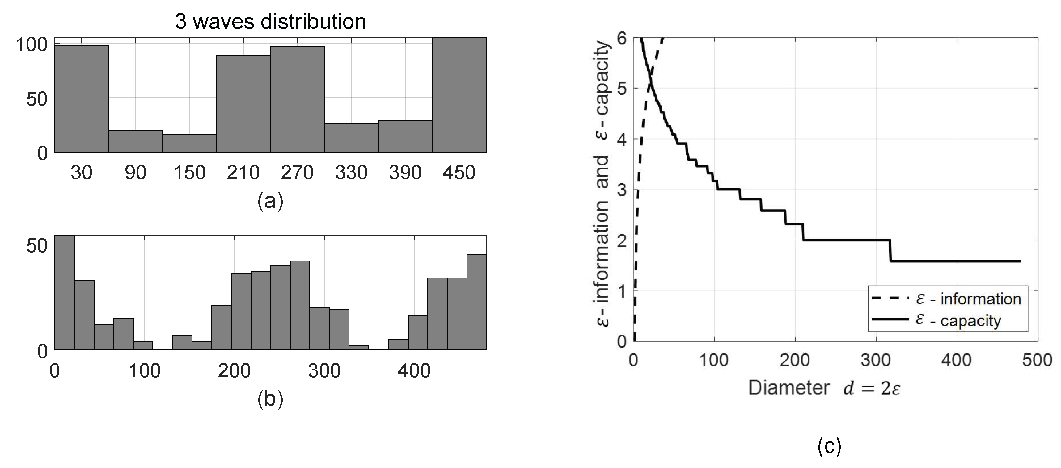
Assume that the office, where the mentioned above clerk works, serves clients hours during a day. Also, assume that the clients arrive by three “waves” – in the morning, in the midday and in the evening.
For this data, diameter calculated by the suggested method and bin lengths calculated by the known rules are the following:
Histogram for this data with the bin lengths calculated using the Scott rule is shown in Figure 3.a, and histogram with the bin lengths calculated by the suggested method is shown in Figure 3.b.
Dependence of the functions and on for this distribution is shown in Figure 3.c.
It is seen that for this data the suggested method results in the diameter which is close to the bin length provided by the simplest rule. Following this result, arrival rates during a day should be calculated each minutes, while the Sturges rule they should be calculated each minutes, by the Scott rule – each minutes, and by the Freedman-Diaconis rule – each 66 minutes.
5. Conclusion
In the paper, we suggested a method of discretization of dynamical system basing on its observations. The method results in the partition , which represents the system, and is as close as possible to the observations partition .
The method utilizes the Kolmogorov and Tikhomirov -entropy and -capacity and the Rokhlin distance between partitions.
Along with theoretical results, the method is presented in the form of ready-to-use algorithm.
The suggested method is also useful for definition of the bin lengths of histograms, especially for the datasets with multimodal distributions.
Funding
This research has not received any grant from funding agencies in the public, commercial, or non-profit sectors.
Conflicts of Interest
The authors declare no conflict of interest.
References
- Billingsley P. Ergodic Theory and Information. John Wiley and Sons: New York, 1965.
- Dinaburg E. I. On the relations among various entropy characteristics of dynamical systems. Math. USSR Izvestija, 1971, 5(2), 337-378.
- Freedman, D.; Diaconis, P. On the histogram as a density estimator: L2 theory. Zeit. Wahrscheinlichkeitstheorie und Verwandte Gebiete, 1981, 57, 453–476. [Google Scholar] [CrossRef]
- Gross D., Shortle J. F., Thompson J. M., Harris C.M. Fundamentals of Queueing Theory, 4th ed. John Wiley & Sons: Hoboken, NJ, 2008.
- Jacod J., Protte P. Discretization of Processes. Springer: Berlin, 2012.
- Kolmogorov A., N.; Tikhomirov V., M. ε -entropy and ε -capacity of sets in functional spaces. Amer. Mathematical Society Translations, Ser. 2 1961, 17, 277–364. [Google Scholar]
- Martin N., England J. Mathematical Theory of Entropy. Cambridge University Press: Cambridge, UK, 1984.
- Reis Y. Private conversation. Ariel University, Ariel, March 2024.
- Rokhlin V. A. New progress in the theory of transformations with invariant measure. Russian Mathematical Surveys, 1960, 15(4), 1–22.
- Schwarz G. Estimating the dimension of a model. Annals of Statistics, 1978, 6(2), 461-464.
- Scott D., W. On optimal and data-based histograms. Biometrika, 1979, 66, 605–610. [Google Scholar] [CrossRef]
- Sinai Y. G. Introduction to Ergodic Theory. Princeton University Press: Princeton, 1976.
- Sinai Y. G. Topics in Ergodic Theory. Princeton University Press: Princeton, 1993.
- Sturges, H. The choice of a class-interval. J. Amer. Statistics Association, 1926, 21, 65–66. [Google Scholar] [CrossRef]
- Vitushkin A. G. Theory of Transmission and Processing of Information, Pergamon Press: New York, 1961.
Figure 1.
Dependence of -information and -capacity on the diameter of the sets for the partition , , , , where points are evenly distributed on the interval , , . The step is .
Figure 1.
Dependence of -information and -capacity on the diameter of the sets for the partition , , , , where points are evenly distributed on the interval , , . The step is .
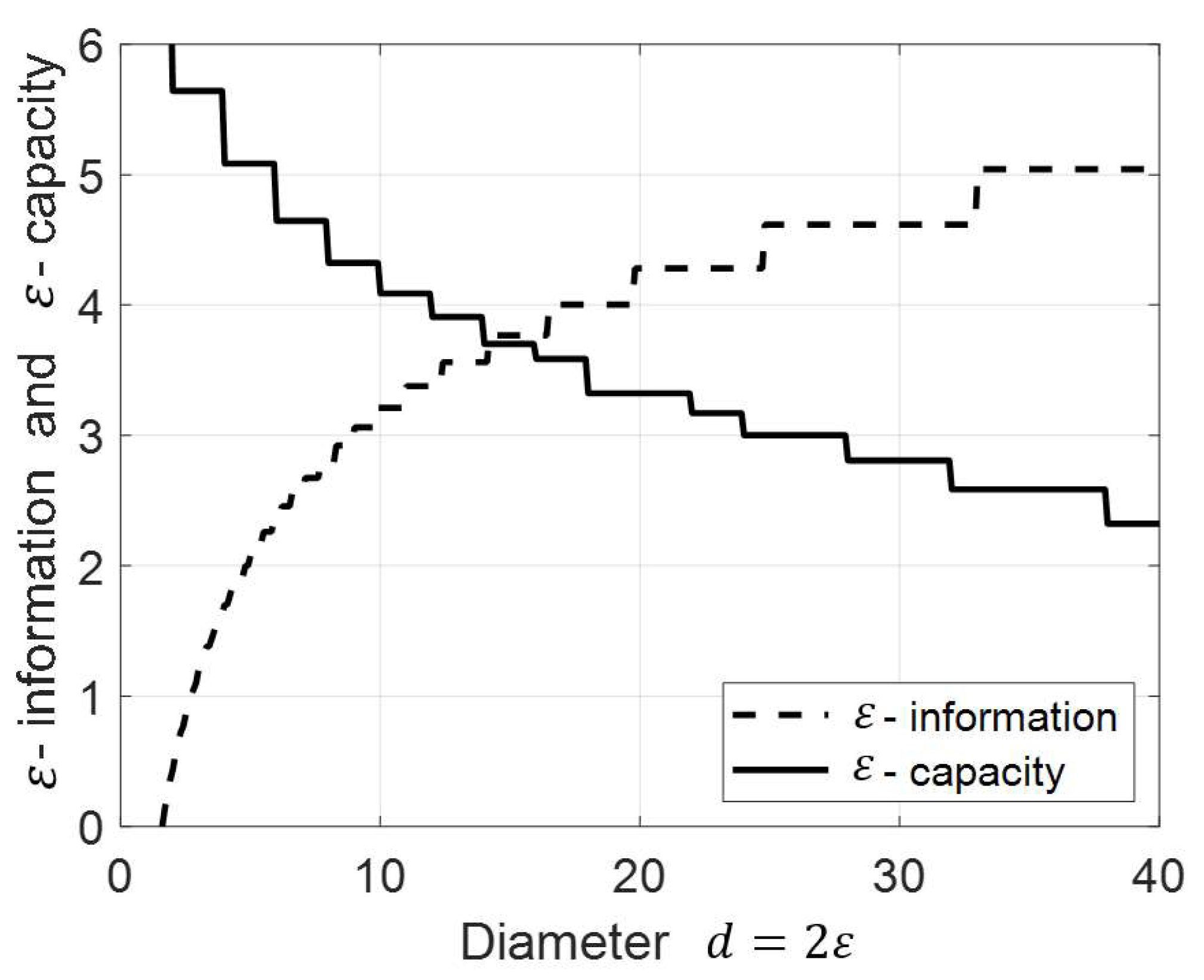
Figure 2.
Histograms plotted using the bin lengths calculated using the Scott rule (figures (a) for each distribution) and using the bin lengths calculated using the suggested method (figures (b) for each distribution).
Figure 2.
Histograms plotted using the bin lengths calculated using the Scott rule (figures (a) for each distribution) and using the bin lengths calculated using the suggested method (figures (b) for each distribution).
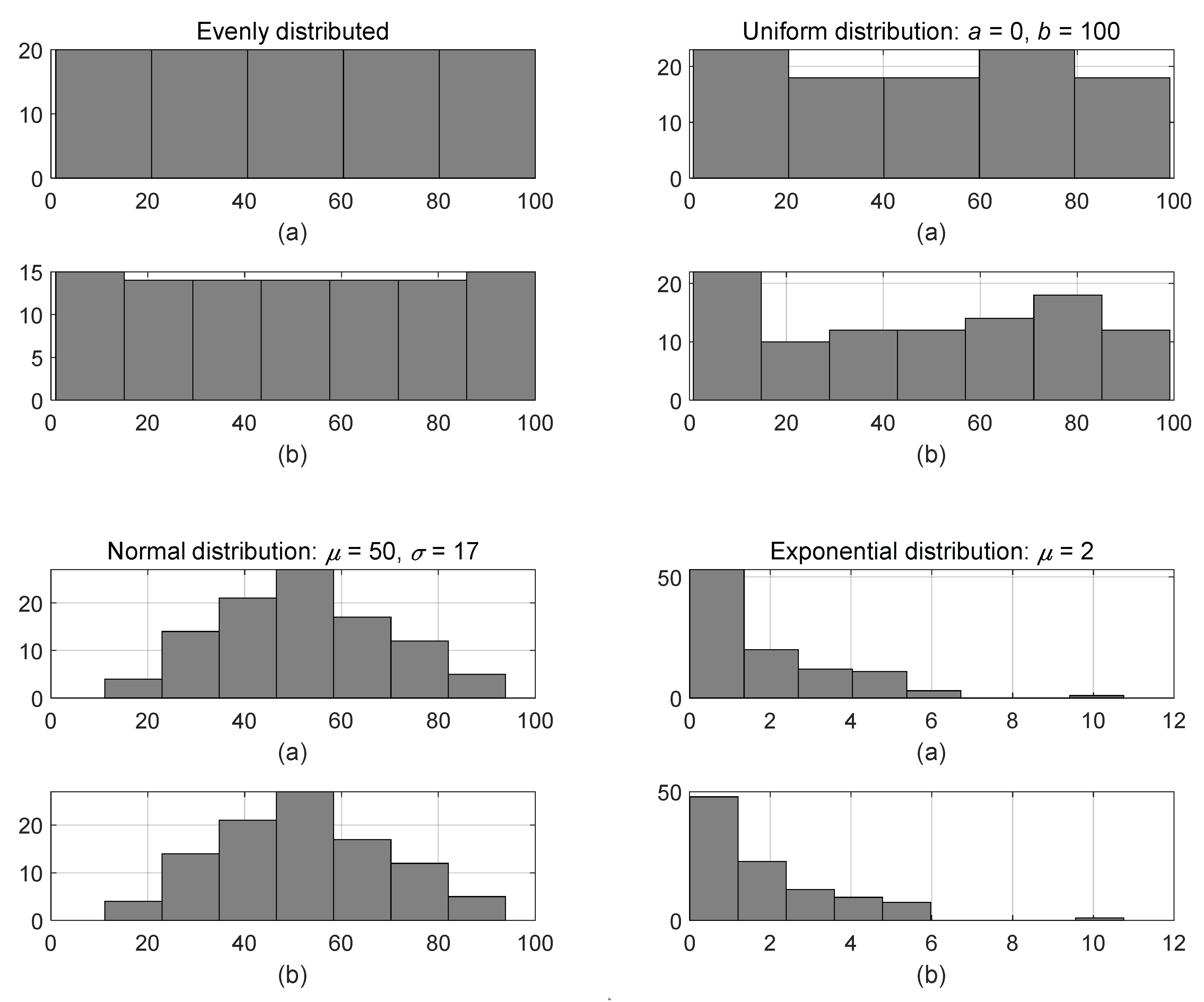
Figure 3.
Arrivals of the clients during a day: (a) histogram with the bin length computed by the Scott rule; (b) histogram with the bin length computed by the suggested algorithm; (c) dependences of -information and -capacity on the diameter .
Figure 3.
Arrivals of the clients during a day: (a) histogram with the bin length computed by the Scott rule; (b) histogram with the bin length computed by the suggested algorithm; (c) dependences of -information and -capacity on the diameter .
Disclaimer/Publisher’s Note: The statements, opinions and data contained in all publications are solely those of the individual author(s) and contributor(s) and not of MDPI and/or the editor(s). MDPI and/or the editor(s) disclaim responsibility for any injury to people or property resulting from any ideas, methods, instructions or products referred to in the content. |
© 2024 by the authors. Licensee MDPI, Basel, Switzerland. This article is an open access article distributed under the terms and conditions of the Creative Commons Attribution (CC BY) license (http://creativecommons.org/licenses/by/4.0/).
Copyright: This open access article is published under a Creative Commons CC BY 4.0 license, which permit the free download, distribution, and reuse, provided that the author and preprint are cited in any reuse.


