
Submitted:
06 September 2024
Posted:
06 September 2024
You are already at the latest version
Abstract
Unmanaged forest ecosystems play a critical role in addressing the ongoing climate and biodiversity crises. As there is no commercial interest in monitoring the health and development of such inaccessible habitats, low-cost assessment approaches are needed. We used a method combining RGB imagery acquired using an Unmanned Aerial Vehicle (UAV), Sentinel-2 data and field surveys to determine the carbon stock of an unmanaged forest in the UNESCO World Heritage Site wilderness area Dürrenstein-Lassingtal in Austria. The entry-level consumer drone (DJI Mavic Mini) and free of charge Sentinel-2 multispectral datasets were used for the evaluation. We merged the Sentinel-2 derived vegetation index NDVI with aerial photogrammetry data and used an orthomosaic and a Digital Surface Model (DSM) to map the extent of woodland in the study area. The Random Forest (RF) Machine Learning (ML) algorithm was used to classify land cover. Based on the acquired field data, the average carbon stock per hectare of forest was determined to be 371.423 ± 51.106 t of CO2 and applied to the ML-generated classification. An overall accuracy of 80.8% with a Cohen’s kappa value of 0.74 was achieved for the land cover classification, while the carbon stock of the living Above-Ground Biomass (AGB) was estimated with an accuracy of -1.0% (± 5.9%). In conclusion, the proposed approach demonstrated that the combination of low-cost remote sensing data and field work can predict above-ground biomass with high accuracy. The results and the estimation error distribution highlight the importance of accurate field data.
Keywords:
UAV
; Sentinel-2
; RGB imagery
; NDVI
; random forest
; carbon storage capacity
; near-natural forest
; wilderness area
; Austria
1. Introduction
Unmanaged forests are critical for climate change mitigation and biodiversity conservation, but monitoring these often-inaccessible areas requires cost-effective approaches [1]. They are a refuge for endangered species and absorb significant amounts of carbon dioxide (CO2) from the atmosphere [2]. In Europe, less than 3% of the entire woodland can be described as primary or old-growth forest [3]. The ongoing climate crisis, deforestation and loss of biodiversity have increased the attention paid to these habitats [3]. Until a few years ago it was believed that old-growth forests stop accumulating carbon as soon as they have reached a certain age and become carbon neutral [1]. This widely accepted assumption was mainly based on data from a single site researched by Kira et al. [1,4] and was first challenged by Luyssaert et al. [1] in 2008. Recent discoveries suggest that the carbon storage capacity of unmanaged near-natural forests has been underestimated for decades [1,5,6,7,8]. If protection and restoration measures were taken, global forests would have the potential to store additional 226 Gt of carbon in areas with low human influence [5]. As this can only be achieved in intact ecosystems, these environments are becoming increasingly relevant for meeting global climate and biodiversity goals [5]. Considering and monitoring the carbon storage capacity and the condition of old-growth and unmanaged forests becomes vital for understanding the influence of climate change on the carbon sequestration of woodlands [9]. As global warming will affect the carbon stock of forests in the next few years, we need to know the exact state of these habitats [9,10].
Knowledge about the current condition of primary and mature unmanaged forests in Europe is poor [11]. Near-natural forests in Europe are in remote and often inaccessible terrain. This inaccessibility has always been the main factor that has ensured the survival of these habitats. Due to the difficult terrain, it is very challenging to carry out extensive in-situ measurements. Because of their spatial isolation, these woodlands are of no commercial interest. Their remoteness further limits the time and budget available for conventional assessments. Innovative low-cost monitoring techniques allow to assess the condition and the extent of primary and unmanaged near-natural forests [12].
Remote sensing is a potent alternative or at least a complement to traditional forest inventories in estimating Above-Ground Biomass (AGB). As there is no commercial interest in most primary and near-natural forests, the method needs to be budget-friendly. Most studies about near-natural forests resort to conventional remote sensing forestry methods [11]. Established approaches use Airborne Laser Scanning (ALS), multispectral satellite imagery or Unmanned Aerial Vehicle (UAV) imagery and focus on the estimation of AGB and its correlation with the carbon storage capacity of the whole trees [13,14,15,16,17,18]. The remote sensing approaches discussed herein aim to solely quantify the AGB of the areas studied, as the findings from Neumann, Echeverria [19] imply that the approximation of the carbon sink capacity of deadwood is highly complex and requires further research.
ALS data is regularly used to determine the structural parameters of forests. With its unique ability to penetrate existing vegetation, it can be used to generate a three-dimensional model of the scanned woodland. Combined with high-resolution multispectral imagery, this approach provides detailed information about the structure of forests [11]. ALS is capable of approximating the AGB with high accuracy even in dense forests [21]. However, combining ALS data with high-resolution multispectral imagery is expensive and requires various hard- and software resources to process the acquired information [11].
In contrast to ALS and high-resolution multispectral imagery, the acquisition of visible light (RGB) images is more efficient. Advancements in UAV technology have made high-resolution RGB imagery more affordable and have improved the technology’s availability. The lack of additional bands makes the classification of different types of land cover using this type of sensor spectrally less accurate and represents a significant shortcoming of this technology. Furukawa, Laneng [20] have proved that UAV derived RGB imageries are nevertheless viable to monitor vegetational changes.
In recent years, multispectral satellite imagery has been used to monitor unmanaged and near-natural forests on a large scale. Spracklen and Spracklen [21] demonstrated that Sentinel-2 images can be used to detect European primary forests with high accuracy. The biggest advantages of this technology are its availability and scalability, as it is viable for monitoring woodlands on a continental scale. Due to its comparably low resolution, it cannot be used to detect smaller changes in the existing vegetation [22].
New findings suggest that the combination of high-resolution RGB imagery, multispectral satellite imagery, Digital Surface Models (DSM) and supervised Machine Learning (ML) can be used to detect tree canopy cover with high accuracy [23,24]. In recent years, the Random Forest (RF) algorithm has been increasingly recognized in the field of remote sensing [5,13,25,26,27,28]. This supervised ML method delivers more robust results when evaluating multidimensional datasets than its competitors [25,26]. RF has been used in numerous remote sensing studies and applications, as well as to detect and monitor old-growth and near-natural forests [5,13,21,25,26,27,28].
When combined with remote sensing techniques, in-situ measurements are only required for initial calibration and validation purposes when assessing woodlands [13]. This principle also applies to carbon stock estimations derived from remote sensing data [29]. As there is hardly any detailed information on the condition and extent of unmanaged forests, the combination of sample field surveys and remote sensing techniques is a viable approach to monitor these habitats in a time-sensitive manner [16].
This study proposes a low-budget approach to approximate the carbon stock of unmanaged forests in remote locations using a combination of UAV RGB imagery, multispectral satellite imagery and field data. In-situ measurements are used to determine the carbon storage capacity of the live tree biomass per square meter (m²) and assess the accuracy of the approximation.
In summary, the main objective of this study is to propose a low-budget approach to estimate the carbon stock of unmanaged forests in inaccessible areas combining field data and remote sensing techniques. The carbon storage capacity of the live tree biomass is estimated based on the sample data derived from the in-situ measurements. Lastly, the estimated storage capacity is validated against the results of a conventional field-based inventory.
2. Materials and Methods
2.1. Study Area
The study area is located in the UNESCO World Heritage Site wilderness area Dürrenstein-Lassingtal [30] in Austria. Situated in the province of Lower Austria, this protected site includes the largest remaining old-growth forest of the European Alps. Since the establishment of the wilderness area in the years 1997 to 2001 (since 2003 IUCN Ia + Ib), the area’s existing forests have remained unmanaged. Due to legal restrictions, the area of interest is not located in a virgin forest. The study area is at the center of the wilderness area and covers roughly 5.76 ha. It is surrounded by mountains and lies between 700 and 750 m above sea level. In the area of interest (Figure 1, different types of unmanaged and near-natural forests, grassland and bare gravel can be found.
2.2. Field Data
As there is no internationally standardized approach to establishing forest inventories (NFIs) in Europe, the here described methodology tries to strike a balance between the different methods [11,31]. For the sample plots, circular plots with a minimum size of 0.03 ha were defined. To select the survey plots, a fishnet of 20 x 20 m was laid over the study area. Each cell that is covered by woodland was marked as forest. Only sections with at least 30% tree cover were marked [32]. Ten sample plots were randomly distributed across the defined woodland. Figure 2 shows the locations of the sample plots [12].
The in-situ measurements were carried out on three days in September 2023 relying on well-established forest monitoring techniques [11]. We used the software ArcGIS Field Maps (Environmental Systems Research Institute, Inc., Redlands, California) to document the parameters height (H), diameter at breast height (DBH), species and location for every tree [15]. Every tree with a DBH of more than 1 cm was measured. Height values were derived using a Forestry Pro II laser ranger (Nikon Corporation, Tokyo, Japan), while the diameter at breast height was measured using a tree caliper at a stem height of 130 cm. The species of the sampled trees was determined on site by professional foresters and experts. As the study area is located at the bottom of a valley and overshadowed by mountains, we did not use the Global Navigation Satellite System (GNSS) localization feature of Field Maps. The central points of the in-situ plots were located using a print of a high resolution orthophoto and the position of the corresponding point [16]. In total, we recorded 511 trees in the field survey.
2.2. Remote Sensing Data
2.1.1. RGB UAV Imagery
For the acquisition of the high-resolution RGB imagery, we used a DJI Mavic Mini (SZ DJI Technology Co., Shenzhen, China). Based on its specifications (Table A1), the Mavic Mini consumer grade quadcopter can be categorized in the entry-level segment, as it is equipped with a 12 Megapixel RGB sensor. It provides a cost-effective solution for capturing aerial imagery.
Aerial images of the study area were acquired on August 4th, 2023. The Drone Link Premium (Dronelink LLC, Austin, USA) software was used to set the flight parameters. To ensure a ground sampling distance below 5 cm, the flight altitude was set to 100 m above the starting point. The Drone Link version used does not include a terrain follow option [33]. A total area of 7.6 ha was covered with a front overlap of 90% and a side overlap of 70% [34]. During the acquisition, the camera pitch was permanently set to 90° to ensure a certain amount of overlap per picture [35]. On the day of flight 187 images were obtained. Due to the poor GNSS reception, we used no Ground Control Points (GCPs) [36].
2.1.2. Multispectral Satellite Imagery
A cloud free multispectral image of the study area was acquired using the Sentinel-2 L2A (Level 2A data) data catalog. The selected image was taken on August 13th, 2023, and displays no significant changes in land coverage compared to the drone flight on August 4th. Sentinel-2 datasets consist of 13 different spectral bands with different resolutions [37]. For this study, only the channels red (Band 4) and near-infrared (Band 8), both with a spatial resolution of 10 m, were used [38].
2.2. Data Analysis
2.1.2. Live Tree Above-Ground Biomass (ABG)
For each sample plot, the live tree above-ground biomass was estimated based on the measured tree parameters. For most of the species found in the study area the stem wood volume was determined using Denzin’s standard formula [39]. Equation (1) can only be interpreted as an estimate of the actual AGB, as it was designed to be an approximation [41].
2.1.2. Carbon Stock
To calculate carbon storage capacity, the different tree species were divided into two categories: coniferous and deciduous. The stem volume of each group was summarized for every individual field plot. Firstly, the determined wood volume was converted from the metric unit cubic meter (m³) to dry mass tons (t dm). The conversion factors for each wood category can be found in Table 2. To calculate the mass of the whole tree, including leaves, needles, branches and roots, the stem volume was multiplied with the average expansion ratio factor. Based on the whole biomass of the tree, the corresponding carbon storage capacity was determined [40]. To determine the carbon dioxide storage (CO2) capacity, the carbon stored in the evaluated biomass was multiplied with the commonly used factor of 3.67 [41,42]. Equations (3) and (4) illustrate the calculation of the summarized conversion factors based on Austria’s National Inventory Report [40].
2.1.2. Land Cover Classification
The high-resolution RGB UAV images were processed using Agisoft Metashape (Agisoft LLC., St. Petersburg, Russia) software [20]. Agisoft provides a predefined set of parameters for the generation of Digital Surface Models (DSM) and Orthomosaics without GCPs. The settings (Table A2) used to generate the DSM and the Orthomosaic were derived from the official best-practice guide provided by Agisoft [43]. Figure 3 depicts the generated DSM and the Orthomosaic.
The multispectral satellite images were used to calculate the Normalized Vegetational Index (NDVI) of the study area. Utilizing the red (RED) and near-infrared (NIR) bands of multispectral datasets, this index differentiates green vegetation from the surrounding ground soil [44]. It typically ranges from -1.0 to +1.0 [44]. Figure 4 shows the raster dataset containing the NDVI indices.
Four different composites were created to evaluate the performance and the applicability of the different remote sensing datasets for the classification of unmanaged forests [23,24]. These datasets represent different combinations of the raster datasets used. The different composites and the corresponding bands are listed in Table 3.
The supervised machine learning algorithm RF was used to classify the generated composites. This algorithm is widely used in the field of remote sensing and can achieve good results with subpar training data [5,13,25,26,27,28]. Figure 5 shows the training samples that were created to train the algorithm [45]. The training samples do not cover the area of the field plots.
2.1.2. Carbon Stock Estimation
The field plots 1, 3, 4 and 6 are covered by continuously forested areas consisting of living trees. Only plot 3 includes a small clearing with a reduced vegetation cover. These four plots were used to determine the average storage capacity per square meter (m²) and hectare (ha) of forest. The summarized carbon stock of the selected sample plots was divided by the aggregated area. The total area of the chosen field plots amounts to 1,250.268 m² [16].
The area covered by woodland was extracted from the classification raster and multiplied with the average storage capacity per hectare to approximate the CO2 storage capacity of each sample plot. The carbon stock of the different plots was summarized to calculate the overall carbon storage capacity of the area investigated during the in-situ measurements.
2.2. Accuracy Assessment
2.2.1. Classification Accuracy
An extended version of the training samples dataset was created to reference the classification [25]. The accuracy of the classification was tested with 100 random validation points per class and summarized in a Confusion Matrix table [46,47]. For the creation of the Confusion Matrix, the Image Classification Wizard of ArcGIS Pro was used (Table A4) [45]. The reference dataset and the validation points are depicted in Figure 6.
2.1.2. Accuracy of Estimated Carbon Stock
The accuracy of the carbon stock estimation is determined based on the in-situ measurements from the sample plots depicted in Figure 2. For each plot the approximated carbon storage capacity was compared to the measured storage capacity. The approximated carbon sum was also contrasted with the measured equivalent. Potential differences were quantified in absolute numbers, percentage values and standard error.
3. Results
3.1. Field Data
3.1.1. Above-Ground Biomass
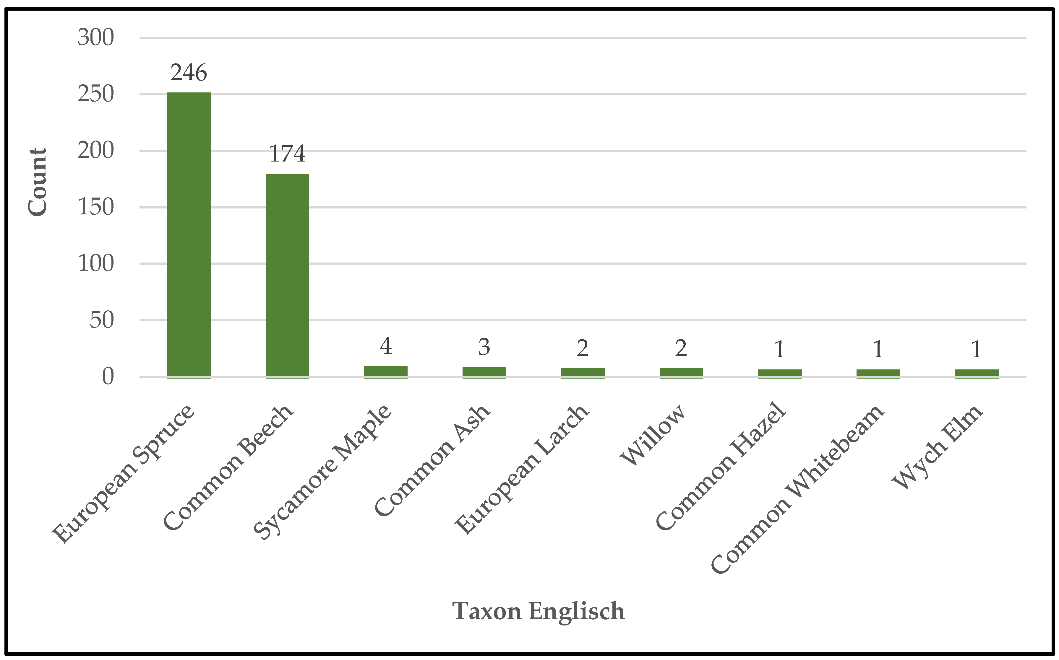
Roughly 85% (434) of the 511 trees sampled are alive. Most of the trees found are European Spruce (56.7%) and Common Beech (40.1%). Other species sampled are European Larch, Common Ash (Fraxinus excelsior), Common Whitebeam (Sorbus aria), Common Hazel (Corylus avellana), Sycamore Maple (Acer pseudoplatanus), Wych Elm (Ulmus glabra) and Willow (Salix).
Figure 7.
Tree species found in the field plots.
All field plots combined contain 65.054 m³ of live tree AGB. With 49.544 m³ (76.2%), most of the biomass surveyed was coniferous wood. 15.511 m³ (23.8%) of the measured live tree biomass was categorized as deciduous wood. The plots 2, 6 and 8 contain the most biomass. These three survey plots are dominated by European Spruce. The plots 1, 3, 4 and 6, used for estimating the average carbon storage capacity, contain 39.186 m³ of live tree biomass. On average, a hectare of continuous forest contains 313.421 ± 44.507 m³ (mean ± standard error) of live tree biomass in the study area.
3.1.2. Carbon Stock
The carbon storage capacity of the forest area found in all field plots amounts to 80.016 t of CO2. With 46.438 t of CO2 (58.04%), most of the carbon stock is located in the sample plots used for the approximation. In the study area, a square meter of forest stores 0.037 ± 0.005 t of CO2, while a hectare of woodland stores 371.423 ± 51.106 t of CO2 on average. Table 4 lists the AGB and carbon stock of each individual field plot.
3.2.Land Cover Classification
The best performing classification raster, as determined based on the datasets orthomosaic, NDVI and DSM, has a resolution of about 3.35 cm and covers the whole study area. With 31,216.412 m² (54.2%), more than half of the study area was classified as Forest. 15,992.287 m² (27,8%) of the area were categorized as Grass, while 7,497.279 m² (13.0%) were covered by Gravel. Only 2,890.393 m² (5.0%) were classified as Deadwood. The configurations of the different composites are depicted in Table 5.
The classification of the study area (Figure 8 achieved an overall accuracy (Total) of 80.8% with a Kappa value of 0.743. In terms of user’s accuracy (U-Accuracy), the Forest category scored 80%. With 62%, the Forest category achieved the worst producer’s accuracy (P-Accuracy) of all four categories. The Deadwood category scored the best result for user’s accuracy (91%) and achieved a P-Accuracy of 81%. The Gravel category achieved the best producer’s accuracy of all four categories (93%) and scored 88% at U-Accuracy. The Grass category achieved the worst user’s accuracy (66%). Table 6 contains the entire Confusion Matrix of the landcover classification raster.
Figure 8.
Classification raster of the study area.
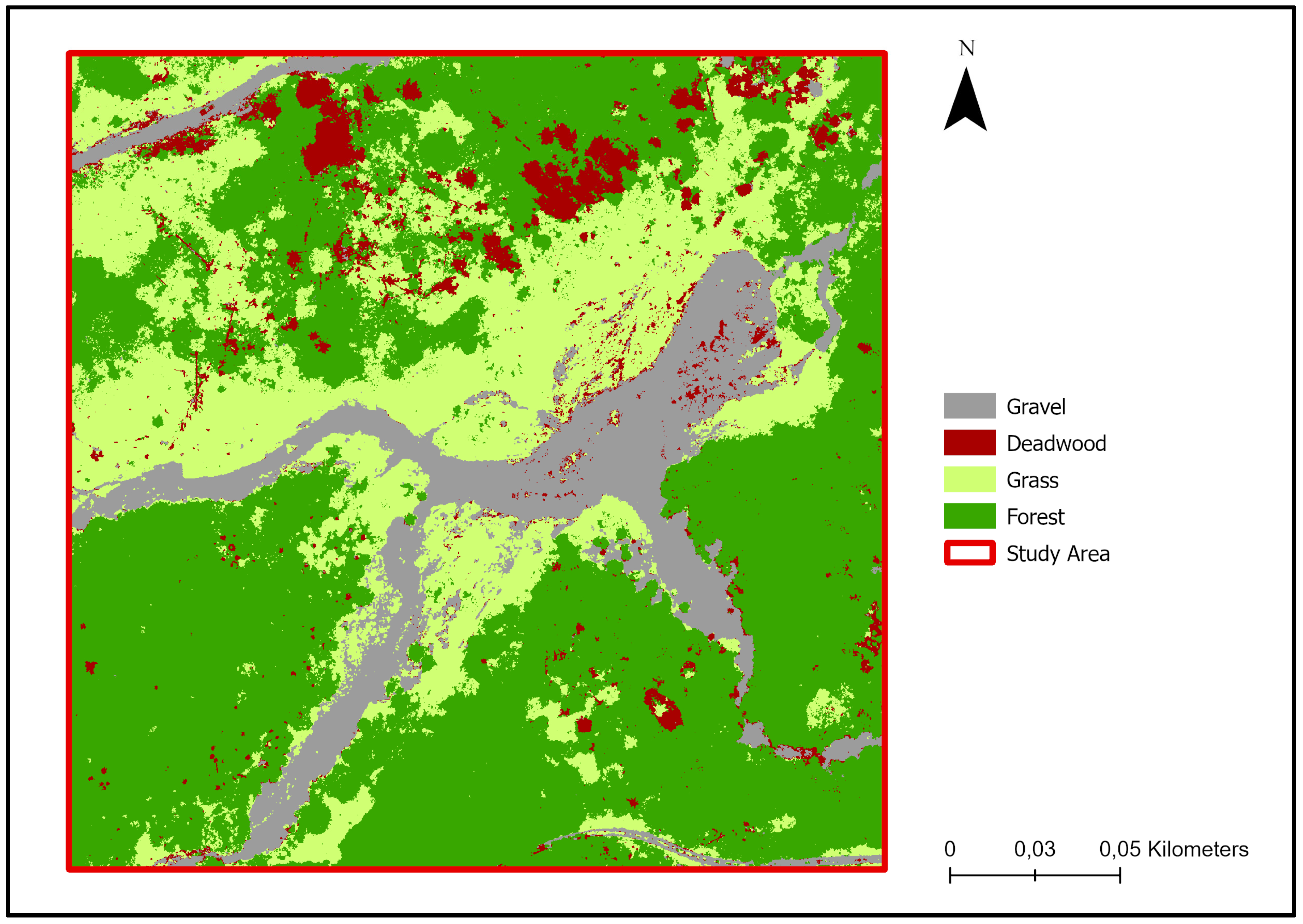
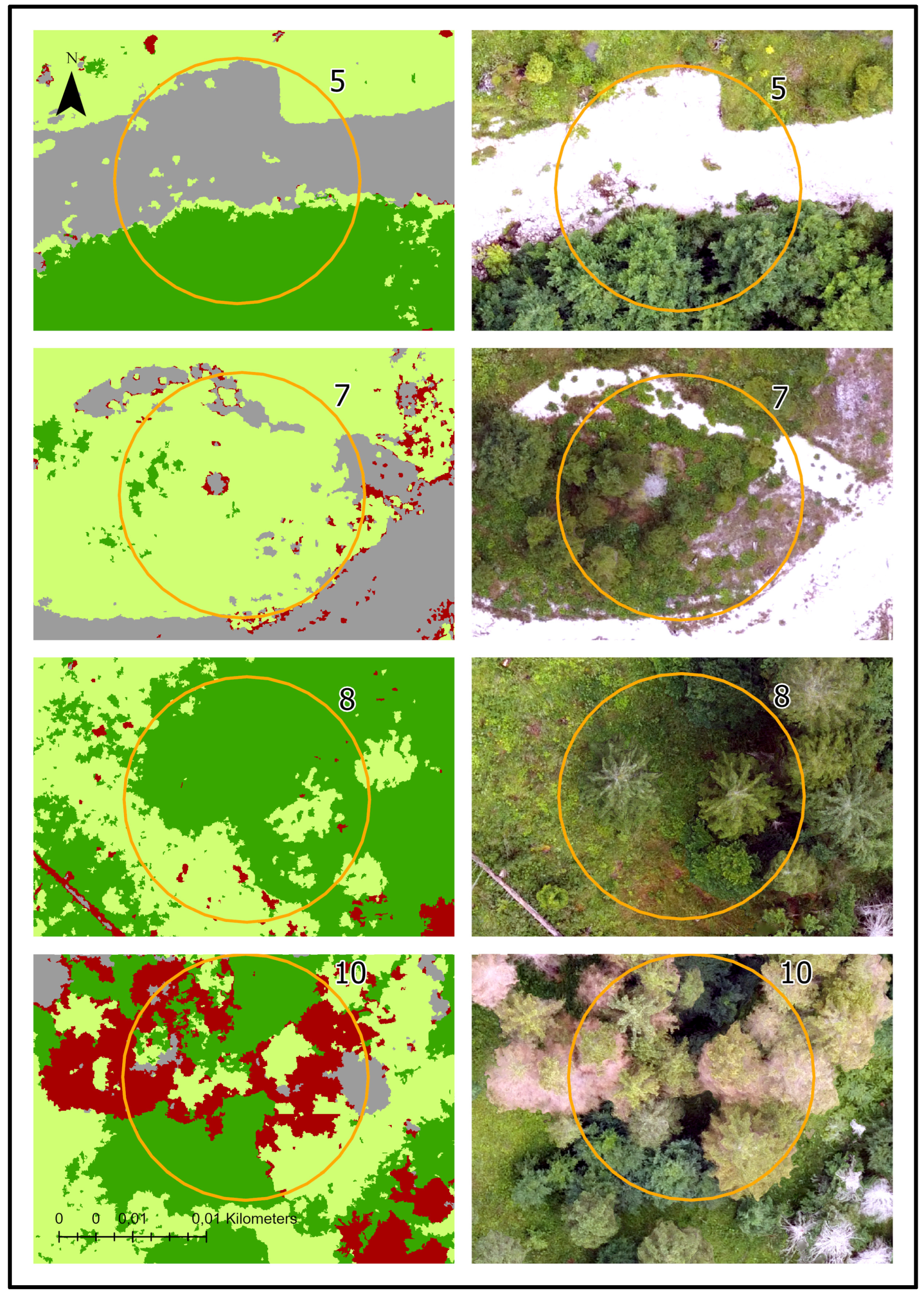
Figure 9 compares the orthomosaic of four sample plots with the land cover classification raster. The focus of this representation lies on the quality of the classification of the Forest, Grass and Deadwood categories.
Figure 9.
Comparison of the land cover classification and the orthomosaic.
3.3. Carbon Stock Estimation
For the field plots, a total carbon storage capacity of 79.186 ± 10.896 t of CO2 was estimated. The approximation of the carbon storage capacity of the field plots (based on the plots 1, 3, 4 and 6) produced an overall error of -0.830 t of CO2 (-1.0%). These four plots were surveyed within six hours during the field work. With a difference of -0.38 t of CO2, the smallest estimation error was achieved for plot 2. The largest error was observed for plot 6 (-11.028 t of CO2). Table 7 lists the estimated carbon stock of the sample plots and the corresponding estimation errors.
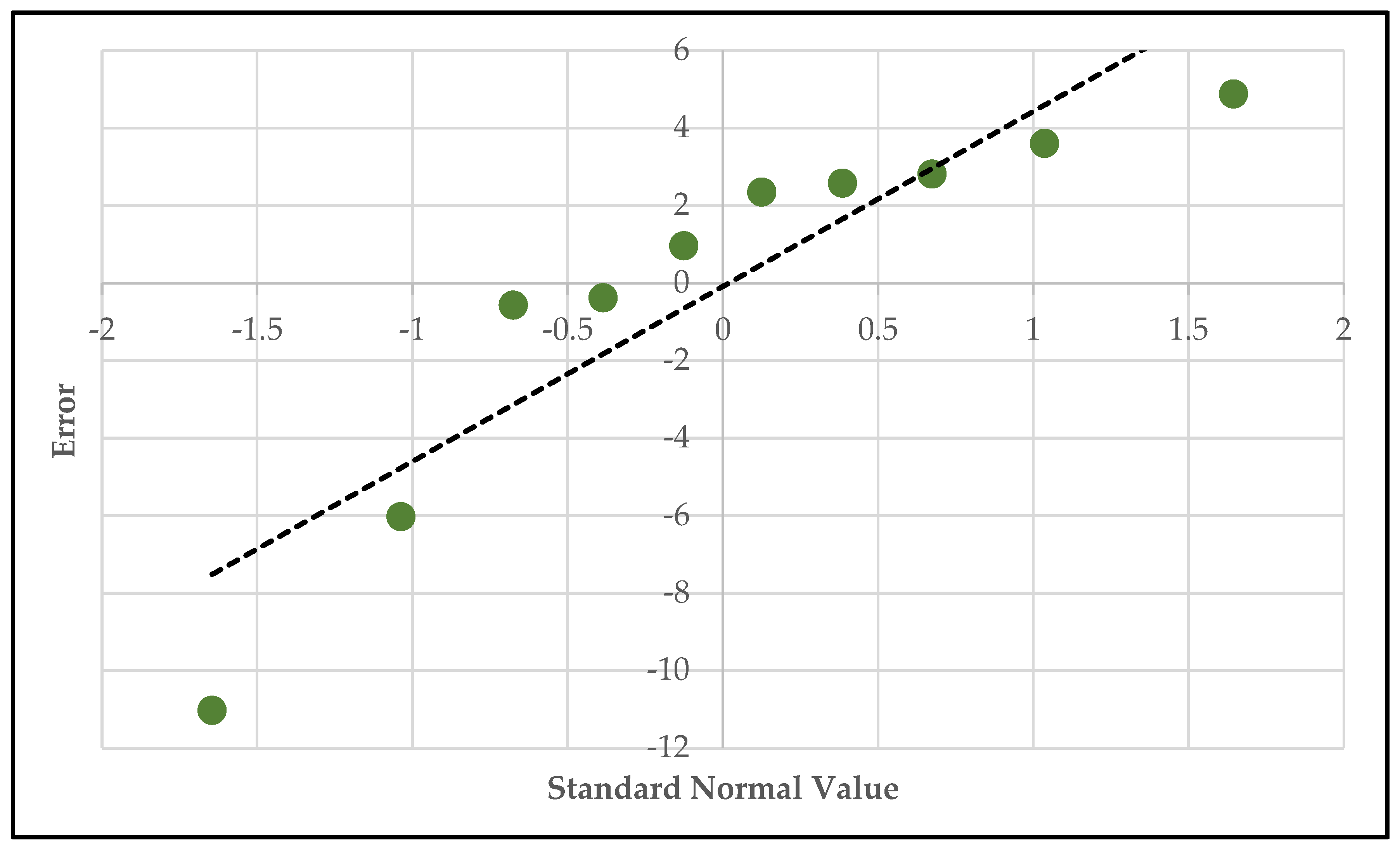
The average error per plot is -0.083 t of CO2, while the standard deviation of the errors amounts to ± 4.648 t of CO2 (± 5.9%). With a median of 1.652 t of CO2 and a skewness of -1.285, the distribution of the errors is skewed to the left. The Pearson kurtosis indicates a peaked distribution with a value of 3.543. Figure 10 is a Quantile-Quantile (Q-Q) plot of the distribution of the carbon stock estimation errors. We assumed a normal distribution to create this chart.
Figure 10.
Q-Q plot of the distribution of the carbon stock estimation errors.
4. Discussion
4.1. Field Data
The structural properties of the researched forest area are similar to those of managed woodlands in Austria. This is not surprising, as the study area incorporates forests that were managed until 2001. More than 85% of the trees found were European Spruce or Common Beech. On average, managed forests in Austria are also dominated by European Spruce (48%) and Common Beech (11%) [48]. With 11%, the share of Common Beech is significantly lower in the managed forests than in the study area [48].
The average live tree AGB derived from the in-situ measurements amounts to 313.421 ± 44.507 m³ ha-1. Considering the altitude of 700 m and the geomorphological structure of the study area, this estimation is also in line with the national average for managed forests with 351 ± 3.3 m³ ha-1 [48]. With 250 to 315 tons of tree biomass at a height of 800 to 900 m above sea level, Duduman et al. [49] came to a similar result in a comparable study area in Romania. The differences in biomass can be explained by the variances in altitude and forest structure, as the altitude of the habitat strongly influences the amount of live tree biomass in alpine regions [49,50].
Based on the measured live tree biomass, the average carbon storage capacity per hectare amounts to 371.423 ± 51.106 t of CO2. This value is in line with the methodology and the conclusions stated in Austria’s Inventory Report 2023 [40].
4.2. Land Cover Classification
Adding the DSM to the orthomosaic improved the overall performance of the classification by 6%. This is a bigger improvement than Schiefer et al. [32] documented in their study, in which they focused on the classification of individual tree species. Al-Najjar et al. [51] stated that the combination of RGB imagery and height information (e.g. DSM) improves the accuracy of vegetation classification by up to 1.8% compared to stratifications based on an orthomosaic.
Combining the orthomosaic and the NDVI indices improved the overall accuracy by 2.3%. Compared to the performance of the composite consisting of the orthomosaic and the DSM, this is a minor enhancement. A study conducted by Daryaei et al. [52] came to the conclusion that high-resolution RGB-imagery combined with canopy height information can detect woodland with a high overall accuracy without Sentinel-2 datasets. This interpretation is concurrent with the findings in this study, although the present study did not incorporate a full canopy height model (CHM).
Adding the NDVI values further enhanced the overall accuracy of the third composite (orthomosaic + DSM) by 0.8%. Daryaei et al. [52] managed to improve the classification accuracy of Sentinel-2 datasets by around 2% using UAV-based datasets. Although the combination of RGB and multispectral datasets did not significantly enhance the overall accuracy, Daryaei et al. [52] also concluded that the combination of high-resolution RGB imagery and vegetational indices based on multispectral satellite data is important for the robustness of the classification of different vegetation classes and tree species.
Today, a wide variety of vegetational indices are in use [15]. For example, the Green Normalized Vegetation Index (GNDVI), NDVI2, the Canopy Chlorophyll Content Index (CCCI) and the Green Leaf Index (GLI) are utilized to evaluate different vegetational parameters [15,23]. As the focus of this study was not the validation of the most meaningful vegetational index, we used the NDVI index, because it is often described as robust and applicable for many different use cases and scenarios [16,21,23,53,54]. Nasiri et al. [23] proved in their study that the NDVI indices, partially derived from the Sentinel-2 datasets (Band 8), are the most important indicators for detecting forest canopy cover. Following work should potentially concentrate on evaluating the influence of the different vegetational indices on the results of the carbon estimation.
With an overall accuracy of 80.8% and a Kappa value of 0.743, the composite consisting of the orthomosaic, NDVI indices and DSM achieved the best result of all four datasets. The results are comparable to those from Heuschmidt et al. [55], who classified cork oak woodlands with an accuracy of 79.5% using images captured by an UAV fitted with an RGB sensor. Another study [56] also achieved 80% classification accuracy with multitemporal airborne RGB images. With 90%, Zhou et al. [57] managed to score a higher overall accuracy for the classification of different vegetation classes using RGB UAV imagery than the methodology described herein. A study conducted by Schiefer et al. [32] classified different tree species with an accuracy of 89% using comparable RGB datasets. Schiefer et al. [32] mentioned that the classification accuracies of different studies cannot be directly compared as various machine learning algorithms and approaches are applied. Nevertheless, most studies using RGB images achieved an accuracy of about 80 to 90% [32,55,56,57]. Thus, the proposed methodology delivered a result that lies within the expected range of accuracy.
Like other studies before, our research has proved that the combination of Sentinel-2 imagery and UAV-derived data is a viable option for detecting and monitoring forest parameters [35,52,58,59]. However, the classification generated in this study does not reach the scientifically accepted total accuracy threshold of 85% and therefore cannot be recommended without further clarification [60,61,62]. As Foody [61] points out, this limit might be too harsh in some cases. Especially distinguishing different types of vegetation can be very challenging without high-resolution multispectral imagery [63]. For example, Ayhan et al. [63] suggest that an overall classification accuracy of about 78% for a high-resolution RGB imagery segmentation should be viewed as sufficient.
The deficits in the overall accuracy of the classification are due to the low user’s and producer’s accuracy in the Forest and Grass classes. The Forest category achieved the overall lowest P-Accuracy value, while the Grass category achieved the worst U-Accuracy score of all four categories. The low producer’s accuracy for the Forest class means that the classifier produces a lot of false negatives (type 2) [64,65,66]. A low U-Accuracy for the Grass category indicates that the classification is not very reliable and produces numerous errors of commission (type 1) [65,66]. As Dash et al. [67] pointed out, the differences between U-Accuracy and P-Accuracy for a single class can be attributed to similarities in the spectral characteristics of the different categories. This effect seems to be exaggerated by the usage of low-resolution Sentinel-2 images and high-resolution RGB images lacking additional spectral information.
Figure 9 proves that during the classification process the distinction between the two different types of vegetation is prone to error. For example, the single trees in plot 7 were categorized as Grass. The detection of single trees also caused problems in other areas. The single tree standing north of plot 7 was not identified correctly. In plot 8, lighter colored trees were mistaken for Grass, while dense and darker shaded vegetation was often wrongly identified as Forest. Komárek et al. [68] stated that the robust classification of similar vegetation types requires high-resolution thermal or multispectral imagery. The study conducted by Furukawa et al. [20] also came to the same conclusion. But as Oddi et al. [69] pointed out, acquiring high-resolution multispectral imagery would be costly and would make the methodology more complicated. Hence, an approach using high-resolution multispectral datasets is not suitable for the use case described herein.
The Deadwood and Gravel classes continuously achieved producer’s and user’s accuracies of more than 80% [70]. Plot 10 in Figure 9 however, shows that the distinction between Gravel and Deadwood is not error-free, either. Some of the standing deadwood was mistaken for gravel. Zielewska-Büttner et al. [71] pinpointed that the distinction between bare-ground and standing deadwood relying on orthophotos and DSM is difficult due to the similarities in their spectral characteristics. Using an uncertainty model (UM) for the classification of the classes Bare Ground, Live, Declining and Dead, Zielewska-Büttner et al. [71] achieved higher scores for P- and U-Accuracy than this study.
4.3. Carbon Stock Estimation
As the here described methodology can be described as a highly generalized approach, it also focusses on minimizing the expected errors in detecting land coverage and AGB estimation. These limitations also mean that the here presented findings may not be applicable to other forest types. Error metrics were chosen that describe the distribution of the different errors for applying the average values for AGB and carbon storage capacity on the broad category Forest. The statistical indicators average error, standard deviation, median, skewness and Pearson Kurtosis as well as the Q-Q-plot aim to document the dispersal of the estimation errors across the heterogeneous sample plots [13]. Our findings show that the high variability of structural parameters of diverse forests results in a strong distribution of the approximation error and requires the here described statistical evaluation to understand the overall estimation error.
With an overall error of about 1%, the carbon storage capacity of the field plots was estimated accurately. The average error per plot for the carbon stock estimation is very low (-0.830 t of CO2), while the calculated standard error (SE) of ± 4.648 t of CO2 (5.9%) can be described as substantial. The carbon stock estimation error varies significantly from plot to plot, which can be attributed to the structural parameters, e.g. sum of AGB and species composition, differing significantly across the study area. The findings of the in-situ measurements also show that the studied forest area is very heterogenous. The key figures median, skewness and Pearson kurtosis indicate that the estimation errors do not describe a perfect Gaussian distribution. Figure 10 verifies this assumption and implies that the error distribution only approximates a standard distribution and varies significantly with the structural parameters of the corresponding sample plot.
For most plots, the carbon storage capacity was slightly overestimated. Only the carbon stock of the densely wooded plots 6 and 8 was significantly underestimated. This discrepancy in the error distribution is the main reason for the low overall estimation error. The heterogeneity of the studied forest area makes the estimation of the carbon storage capacity difficult and requires profound knowledge about the existing live tree biomass. A comparable study also came to the conclusion that precise in-situ measurements are critical for the initial calibration phase of the AGB models for accurately monitoring unmanaged and old growth forests [11].
Since the average carbon storage capacity is assigned to the broad vegetation class Forest per unit area (m²), the estimated average value plays a critical role in the estimation. If the in-situ data is sufficiently representing the structural complexity of the study area, the proposed methodology proves to be capable of achieving statistically significant outcomes. While the proposed method works well for the surveyed area, it requires meaningful validation data. More complex or detailed scenarios may require a different approach if fewer field and validation data is available. For example, Fernandes et al. [16] used multispectral images to categorize individual tree species to estimate live tree AGB and carbon stock of riparian woodlands. As Austria’s National Inventory Report [40] proposes, a distinction between coniferous and deciduous species allows for more robust carbon stock estimations. This may be necessary for fully automated approaches, as unmanaged forests are dynamic ecosystems that consist of a wide variety of habitats.
4.4. Cost and Time Expenditure
The methodology described herein focuses on reducing expenses while producing meaningful results. However, the costs of regular ArcGIS Pro and Metashape licenses are substantial [72,73]. In this case, Metashape and ArcGIS Pro were used to ensure the compatibility of the proposed approach with the tools that were already in use for managing the wilderness area. The cost of the hardware used for the evaluation and the number of working hours were also not included, as these values are highly dependent on the size of the study area. Compared to the prices of LiDAR [74] and multispectral UAVs [75], the cost for this approach is significantly lower. Table 8 lists the expenses of the study.
To reduce expenditures for the necessary software products, free of charge open-source software, such as QGIS or OpenDroneMap, can be used for the methodology described herein [79,80]. Using open-source software would also improve the general availability of the proposed approached and potentially lead to an extensive and interoperable database regarding near-natural forests [81].
5. Conclusions and Outlook
The study area in the UNESCO World Heritage Site wilderness area Dürrenstein-Lassingtal [30] had similar AGB and carbon stock characteristics as a typical managed forest in Austria. Combining field data, UAV-derived datasets and Sentinel-2 satellite imagery proved to be an efficient option for estimating the carbon stock of unmanaged forests. With an overall accuracy of 80.8%, the land cover classification based on a composite consisting of high-resolution RGB imagery, DSM and NDVI indices proves to be a reliable basis for carbon stock estimation. The combined carbon storage capacity of the surveyed field plots was underestimated by 1%. Due to the high variability of carbon stock found in the study area, the SE of the estimated storage capacity of ± 10.896 t of CO2 (± 13.6%) and the SE of the overall estimation error of ± 4.648 t of CO2 (± 5.8%) provide a better understanding of the accuracy that can be achieved by the proposed approach. The uncertainty illustrated by these values is due to the fact that the average carbon storage capacity is applied to the whole area covered by woodland.
“The studied near-natural forest is characterized by a high spatial variability. Topographic trends are effecting the structural properties of the forest. This indicates that the distribution of the sample plots has an impact on the estimation of the carbon storage capacity of the in-situ measurements. As field data is essential for the here proposed approach, further investigation is necessary to improve the in-situ protocol. A possible solution to improve the selection of sample plots for large-scale forest inventories was proposed by Pohjankukka et al. [82], where remote sensing data and machine learning technologies were synthesized to improve the field survey.”
Future work should focus on the classification of different woodland types and tree species of unmanaged forests. A distinction between coniferous and deciduous trees, as applied in Austria’s National Inventory Report [40], would allow for a carbon stock analysis based on the specific carbon storage capacities of the different wood categories. A multitemporal approach, such as the methodology proposed by Grybas et al. [82], may allow to accurately detect tree species with consumer-grade UAVs. Current progress in the field of UAV technology improves the availability of high-resolution multispectral imagery via new platforms like the DJI Mavic 3(M) Multispectral [83] and allows for more in-depth land cover assessments [84].
The estimation of the existing AGB could be further enhanced by detecting the individual tree crowns [85,86]. In their studies, Hemery et al. [87] and Iizuka et al. [24] proved that the DBH of different tree species can be derived from the diameter of the tree crown. Buchacher et al. [88] developed a methodology to specifically estimate the crown width of different trees in species-rich Austrian woodlands. Another study [86] concluded that the strong correlation between the AGB and the crown diameter and tree height parameters can be used to accurately estimate the existing tree biomass.
The above-mentioned approaches can further reduce the need for field data and improve the approximation of AGB carbon storage capacity. These approaches can therefore be used to further enhance the methodology proposed herein. Future research should therefore focus on the implementation of the mentioned concepts.
Author Contributions
Conceptualization, Thomas Leditznig and Hermann Klug; methodology, Thomas Leditznig; software, Thomas Leditznig; validation, Thomas Leditznig; formal analysis, Thomas Leditznig; investigation, Thomas Leditznig; resources, Thomas Leditznig; data curation, Thomas Leditznig; writing—original draft preparation, Thomas Leditznig; writing—review and editing, Thomas Leditznig and Hermann Klug; visualization, Thomas Leditznig; supervision, Hermann Klug; project administration, Thomas Leditznig and Hermann Klug. All authors have read and agreed to the published version of the manuscript.
Funding
This research received no external funding.
Data Availability Statement
The original data presented in the study are openly available here: 10.5281/zenodo.11657557.
Acknowledgments
My thanks go to Christoph Leditznig, Lara Eigner and Marlon Schwienbacher for their input on the in-situ measurements and the field plots. Furthermore, I would also like to thank Anna Lienbacher, Stefan Mayer and Verena Brinda for proofreading the final manuscript and pointing out potential errors.
Conflicts of Interest
The authors declare no conflicts of interest. The funders had no role in the design of the study; in the collection, analyses or interpretation of data; in the writing of the manuscript; or in the decision to publish the results.
Appendix A

Table A1.
DJI Mavic Mini specifications.
| Takeoff Weight | 249 g |
| Hovering Accuracy Range | Vertical: ±0.1 m (with Vision Positioning), ±0.5 m (with GPS Positioning) Horizontal: ±0.3 m (with Vision Positioning), ±1.5 m (with GPS Positioning) |
| Sensor | 1/2,3’‘ CMOS |
| Effective Pixels | 12 Megapixel |
| Focal Length | 4,4 mm |
| Aperture | f/2,8 |
| Austrian MSRP (November 2019) | 399 € |
Table A2.
Parameters used for the generation of the DSM and the Orthomosaic in Agisoft Metashape.
| Processing step | Parameter | Value |
|---|---|---|
| Align Photos | Accuracy | High |
| Generic preselection | Yes | |
| Reference preselection | Source | |
| Key point limit | 40,000 | |
| Tie point limit | 10,000 | |
| Optimize Camera Alignment | General | F, k1, k2, k3, k3, cx, cy, p1, p2, b1, b2 |
| Build Point Cloud | Quality | High |
| Depth filtering | Mild | |
| Calculate point colors | Yes | |
| Calculate point confidence | Yes | |
| Build DEM | Type | Geographic |
| Coordinate System | WGS 84 (EPSG::4326) | |
| Source data | Point cloud | |
| Interpolation | Enabled (default) | |
| Resolution (m) | 0.0802 | |
| Total size (pix) | 5836 x 5039 | |
| Build Orthomosaic | Type | Geographic |
| Coordinate System | WGS 84 (EPSG: 4326) | |
| Surface | DEM | |
| Blending mode | Mosaic (default) | |
| Enable hole filing | Yes | |
| Total size (pix) | 10,772 x 10,078 | |
| Export DEM | Coordinate System | WGS 84 (EPSG::4326) |
| Raster transform | None | |
| Write tiled TIFF | Yes | |
| Generate TIFF overviews | Yes |
Table A3.
Parameters used to classify the composite raster.
| Processing step | Parameter | Value |
|---|---|---|
| Training Samples Manager | New Schema (Class) | Deadwood, Forest, Grass, Gravel |
| Configure | Classification Method | Supervised |
| Classification Type | Object based | |
| Segmentation | Spectral detail | 16.00 |
| Spatial detail | 17 | |
| Minimum segment size in pixels | 20 | |
| Train | Classifier | Random Trees |
| Maximum Number of Trees | 60 | |
| Maximum Tree Depth | 30 | |
| Maximum Number of Samples per Class | 17,500 | |
| Segment Attributes | Active chromaticity color, Mean digital number, Compactness |
Table A4.
Composites with the corresponding datasets and bands.
| Processing step | Parameter | Value |
|---|---|---|
| Accuracy Assessment | Number of Random Points | 400 |
| Sampling Strategy | Equalized Stratified Random |
References
- Luyssaert, S., et al., Old-growth forests as global carbon sinks. Nature, 2008. 455(7210): p. 213-215.
- Paillet, Y., et al., Biodiversity Differences between Managed and Unmanaged Forests: Meta-Analysis of Species Richness in Europe. Conservation Biology, 2010. 24(1): p. 101-112.
- José I. Barredo, C.B., Anne Teller, Francesco Maria Sabatini, Achille Mauri, Klara Janouskova, Mapping and assessment of primary and old-growth forests in Europe. 2021.
- Kira, T., Tsunahide, Shidei, Primary production and turnover of organic matter in different forest ecosystems of the western Pacific. Japanese Journal of Ecology, 1967. 17.2: p. 70-87.
- Mo, L., et al., Integrated global assessment of the natural forest carbon potential. Nature, 2023. 624(7990): p. 92-101.
- McGarvey, J.C., et al., Carbon storage in old-growth forests of the Mid-Atlantic: toward better understanding the eastern forest carbon sink. Ecology, 2015. 96(2): p. 311-317.
- Yang, Y., Y. Luo, and A.C. Finzi, Carbon and nitrogen dynamics during forest stand development: a global synthesis. New Phytologist, 2011. 190(4): p. 977-989.
- Jacob, M., et al., Significance of Over-Mature and Decaying Trees for Carbon Stocks in a Central European Natural Spruce Forest. Ecosystems, 2013. 16(2): p. 336-346.
- Chiti, T., et al., The potential for an old-growth forest to store carbon in the topsoil: A case study at Sasso Fratino, Italy. Journal of Forestry Research, 2024. 35(1).
- Dean, C. and G. Wardell-Johnson, Old-growth forests, carbon and climate change: Functions and management for tall open-forests in two hotspots of temperate Australia. Plant Biosystems - An International Journal Dealing with all Aspects of Plant Biology, 2010. 144(1): p. 180-193.
- Hirschmugl, M., et al., Review on the Possibilities of Mapping Old-Growth Temperate Forests by Remote Sensing in Europe. Environmental Modeling & Assessment, 2023. 28(5): p. 761-785.
- Inoue, T., et al., Unmanned Aerial Survey of Fallen Trees in a Deciduous Broadleaved Forest in Eastern Japan. PLoS ONE, 2014. 9(10): p. e109881.
- Lalechere, E., et al., Assessing the potential of remote sensing-based models to predict old-growth forests on large spatiotemporal scales. J Environ Manage, 2024. 351: p. 119865.
- Gao, L. and X. Zhang, Above-Ground Biomass Estimation of Plantation with Complex Forest Stand Structure Using Multiple Features from Airborne Laser Scanning Point Cloud Data. Forests, 2021. 12(12): p. 1713.
- Naik, P., M. Dalponte, and L. Bruzzone, Prediction of Forest Aboveground Biomass Using Multitemporal Multispectral Remote Sensing Data. Remote Sensing, 2021. 13(7): p. 1282.
- Fernandes, M.R., et al., Carbon Stock Estimations in a Mediterranean Riparian Forest: A Case Study Combining Field Data and UAV Imagery. Forests, 2020. 11(4): p. 376.
- Lin, J., et al., Aboveground Tree Biomass Estimation of Sparse Subalpine Coniferous Forest with UAV Oblique Photography. Remote Sensing, 2018. 10(11): p. 1849.
- Ahmad, A., H. Gilani, and S.R. Ahmad, Forest Aboveground Biomass Estimation and Mapping through High-Resolution Optical Satellite Imagery—A Literature Review. Forests, 2021. 12(7): p. 914.
- Neumann, M., S. Echeverria, and H. Hasenauer, A simple concept for estimating deadwood carbon in forests. Carbon Management, 2023. 14(1).
- Furukawa, F., et al., Comparison of RGB and Multispectral Unmanned Aerial Vehicle for Monitoring Vegetation Coverage Changes on a Landslide Area. Drones, 2021. 5(3): p. 97.
- Spracklen, B.D. and D.V. Spracklen, Identifying European Old-Growth Forests using Remote Sensing: A Study in the Ukrainian Carpathians. Forests, 2019. 10(2): p. 127.
- Martinez, J.L., et al., Comparison of Satellite and Drone-Based Images at Two Spatial Scales to Evaluate Vegetation Regeneration after Post-Fire Treatments in a Mediterranean Forest. Applied Sciences, 2021. 11(12): p. 5423.
- Nasiri, V., et al., Modeling Forest Canopy Cover: A Synergistic Use of Sentinel-2, Aerial Photogrammetry Data, and Machine Learning. Remote Sensing, 2022. 14(6): p. 1453.
- Iizuka, K., et al., Estimating Tree Height and Diameter at Breast Height (DBH) from Digital Surface Models and Orthophotos Obtained with an Unmanned Aerial System for a Japanese Cypress (Chamaecyparis obtusa) Forest. Remote Sensing, 2017. 10(2): p. 13.
- Belgiu, M. and L. Drăguţ, Random forest in remote sensing: A review of applications and future directions. ISPRS Journal of Photogrammetry and Remote Sensing, 2016. 114: p. 24-31.
- Saini, R. and S.K. Ghosh. Ensemble classifiers in remote sensing: A review. 2017. IEEE.
- Johansen, K., et al., Predicting Biomass and Yield in a Tomato Phenotyping Experiment Using UAV Imagery and Random Forest. Front Artif Intell, 2020. 3: p. 28.
- Karlson, M., et al., Mapping Tree Canopy Cover and Aboveground Biomass in Sudano-Sahelian Woodlands Using Landsat 8 and Random Forest. Remote Sensing, 2015. 7(8): p. 10017-10041.
- Vicharnakorn, P., et al., Carbon Stock Assessment Using Remote Sensing and Forest Inventory Data in Savannakhet, Lao PDR. Remote Sensing, 2014. 6(6): p. 5452-5479.
- Sachser, F., et al., Differential spatial responses of rodents to masting on forest sites with differing disturbance history. Ecology and Evolution, 2021. 11(17): p. 11890-11902.
- Winter, S., et al., Possibilities for harmonizing national forest inventory data for use in forest biodiversity assessments. Forestry, 2008. 81(1): p. 33-44.
- Schiefer, F., et al., Mapping forest tree species in high resolution UAV-based RGB-imagery by means of convolutional neural networks. ISPRS Journal of Photogrammetry and Remote Sensing, 2020. 170: p. 205-215.
- dronelink. Compare Hobbyist Plans. Available online: https://app.dronelink.com/pricing/hobbyist/compare.
- Jiménez-Jiménez, S.I., et al., Digital Terrain Models Generated with Low-Cost UAV Photogrammetry: Methodology and Accuracy. ISPRS International Journal of Geo-Information, 2021. 10(5): p. 285.
- Dash, J., G. Pearse, and M. Watt, UAV Multispectral Imagery Can Complement Satellite Data for Monitoring Forest Health. Remote Sensing, 2018. 10(8): p. 1216.
- Kapil, R., et al., Orthomosaicking Thermal Drone Images of Forests via Simultaneously Acquired RGB Images. Remote Sensing, 2023. 15(10).
- Phiri, D., et al., Sentinel-2 Data for Land Cover/Use Mapping: A Review. Remote Sensing, 2020. 12(14): p. 2291.
- ESA. Spatial Resolution. Available online: https://sentinels.copernicus.eu/web/sentinel/user-guides/sentinel-2-msi/resolutions/spatial.
- Denzin, A., Schätzung der Masse stehender Waldbäume. Forstarchiv, 1929. 5: p. 382-384.
- Anderl, M., et al., Austria’s National Inventory Report 2023, in Submission under the United Nations Framework Convention on Climate Change. 2023.
- Ganatsas, P., et al., Carbon Pools in a 77 Year-Old Oak Forest under Conversion from Coppice to High Forest. Sustainability, 2022. 14(21): p. 13764.
- Abdullah, M.M., Z.M. Al-Ali, and S. Srinivasan, The use of UAV-based remote sensing to estimate biomass and carbon stock for native desert shrubs. MethodsX, 2021. 8: p. 101399.
- Agisoft. Orthomosaic & DEM generation (without GCPs). 2023. Available online: https://agisoft.freshdesk.com/support/solutions/articles/31000157908-orthomosaic-dem-generation-without-gcps-.
- Tucker, C.J. Red and photographic infrared linear combinations for monitoring vegetation. Remote Sensing of Environment, 1979. 8(2): p. 127-150.
- ESRI. Image Classification Wizard. Available online: https://pro.arcgis.com/en/pro-app/latest/help/analysis/image-analyst/the-image-classification-wizard.htm.
- Bilodeau, M.F., et al., Identifying hair fescue in wild blueberry fields using drone images for precise application of granular herbicide. Smart Agricultural Technology, 2023. 3: p. 100127.
- Lewis, H.G. and M. Brown, A generalized confusion matrix for assessing area estimates from remotely sensed data. International Journal of Remote Sensing, 2001. 22(16): p. 3223-3235.
- Bundesministerium für Land- und Forstwirtschaft, R.u.W. Datensammlung zum Österreichischen Wald. 2023. Available online: https://info.bml.gv.at/themen/wald/wald-in-oesterreich/wald-und-zahlen/waldbericht/datensammlung-zum-oesterrreichischen-wald.html.
- Duduman, G., et al., Aboveground Biomass of Living Trees Depends on Topographic Conditions and Tree Diversity in Temperate Montane Forests from the Slătioara-Rarău Area (Romania). Forests, 2021. 12(11): p. 1507.
- Riihimäki, H., J. Heiskanen, and M. Luoto, The effect of topography on arctic-alpine aboveground biomass and NDVI patterns. International Journal of Applied Earth Observation and Geoinformation, 2017. 56: p. 44-53.
- Al-Najjar, H.A.H., et al., Land Cover Classification from fused DSM and UAV Images Using Convolutional Neural Networks. Remote Sensing, 2019. 11(12): p. 1461.
- Daryaei, A., et al., Fine-scale detection of vegetation in semi-arid mountainous areas with focus on riparian landscapes using Sentinel-2 and UAV data. Computers and Electronics in Agriculture, 2020. 177: p. 105686.
- Huang, X., et al., Estimating Forest Canopy Cover by Multiscale Remote Sensing in Northeast Jiangxi, China. Land, 2021. 10(4): p. 433.
- Tsalyuk, M., M. Kelly, and W.M. Getz, Improving the prediction of African savanna vegetation variables using time series of MODIS products. ISPRS Journal of Photogrammetry and Remote Sensing, 2017. 131: p. 77-91.
- Heuschmidt, F., et al., Cork oak woodland land-cover types classification: a comparison between UAV sensed imagery and field survey. International Journal of Remote Sensing, 2020. 41(19): p. 7649-7659.
- Natesan, S., C. Armenakis, and U. Vepakomma, RESNET-BASED TREE SPECIES CLASSIFICATION USING UAV IMAGES. The International Archives of the Photogrammetry, Remote Sensing and Spatial Information Sciences, 2019. XLII-2/W13: p. 475-481.
- Zhou, R., et al., Object-Based Wetland Vegetation Classification Using Multi-Feature Selection of Unoccupied Aerial Vehicle RGB Imagery. Remote Sensing, 2021. 13(23): p. 4910.
- Puliti, S., et al., Combining UAV and Sentinel-2 auxiliary data for forest growing stock volume estimation through hierarchical model-based inference. Remote Sensing of Environment, 2018. 204: p. 485-497.
- Rossi, F., A. Fritz, and G. Becker, Combining Satellite and UAV Imagery to Delineate Forest Cover and Basal Area after Mixed-Severity Fires. Sustainability, 2018. 10(7): p. 2227.
- McCormic, C.M., Mapping Exotic Vegetation in the Everglades from Large-Scale Aerial Photographs. 1999.
- Foody, G.M., Harshness in image classification accuracy assessment. International Journal of Remote Sensing, 2008. 29(11): p. 3137-3158.
- Anderson, J.R., Hardy, E. E., Roach, J. T. and Witmer, R. E., A Land Use and Land Cover Classification System for Use with Remote Sensor Data. Geological Survey Professional, 1976. Paper 964.
- Ayhan, B. and C. Kwan, Tree, Shrub, and Grass Classification Using Only RGB Images. Remote Sensing, 2020. 12(8): p. 1333.
- Stehman, S.V. and G.M. Foody, Key issues in rigorous accuracy assessment of land cover products. Remote Sensing of Environment, 2019. 231: p. 111199.
- Congalton, R.G., A review of assessing the accuracy of classifications of remotely sensed data. Remote Sensing of Environment, 1991. 37(1): p. 35-46.
- ESRI. Compute Confusion Matrix (Spatial Analyst). Available online: https://pro.arcgis.com/en/pro-app/latest/tool-reference/spatial-analyst/compute-confusion-matrix.htm.
- Dash, P., et al., Improving the Accuracy of Land Use and Land Cover Classification of Landsat Data in an Agricultural Watershed. Remote Sensing, 2023. 15(16): p. 4020.
- Komárek, J., T. Klouček, and J. Prošek, The potential of Unmanned Aerial Systems: A tool towards precision classification of hard-to-distinguish vegetation types? International Journal of Applied Earth Observation and Geoinformation, 2018. 71: p. 9-19.
- Oddi, L., et al., Using UAV Imagery to Detect and Map Woody Species Encroachment in a Subalpine Grassland: Advantages and Limits. Remote Sensing, 2021. 13(7): p. 1239.
- Liu, X., et al., Mapping standing dead trees in temperate montane forests using a pixel- and object-based image fusion method and stereo WorldView-3 imagery. Ecological Indicators, 2021. 133: p. 108438.
- Zielewska-Büttner, K., et al., Detection of Standing Deadwood from Aerial Imagery Products: Two Methods for Addressing the Bare Ground Misclassification Issue. Forests, 2020. 11(8): p. 801.
- Agisoft. Buy - Online Store. Available online: https://www.agisoft.com/buy/online-store/.
- ESRI. ArcGIS Pro Pricing. Available online: https://www.esri.com/en-us/arcgis/products/arcgis-pro/buy#for-business.
- Štroner, M., R. Urban, and L. Línková, A New Method for UAV Lidar Precision Testing Used for the Evaluation of an Affordable DJI ZENMUSE L1 Scanner. Remote Sensing, 2021. 13(23): p. 4811.
- Di Gennaro, S.F., et al., Spectral Comparison of UAV-Based Hyper and Multispectral Cameras for Precision Viticulture. Remote Sensing, 2022. 14(3): p. 449.
- DJI. Specs. 2019. Available online: https://www.dji.com/support/product/mavic-mini.
- Nikon. Forestry Pro II. Available online: https://www.nikon.de/de_DE/product/sport-optics/forestry-pro-ii2.
- Stifter-helfen. ARCGIS PROFESSIONAL ADVANCED. Available online: https://www.stifter-helfen.at/it-spenden/esri/arcgis-professional-advanced.
- Groos, A.R., et al., The Potential of Low-Cost UAVs and Open-Source Photogrammetry Software for High-Resolution Monitoring of Alpine Glaciers: A Case Study from the Kanderfirn (Swiss Alps). Geosciences, 2019. 9(8): p. 356.
- De Luca, G., et al., Object-Based Land Cover Classification of Cork Oak Woodlands using UAV Imagery and Orfeo ToolBox. Remote Sensing, 2019. 11(10): p. 1238.
- Vivar-Vivar, E.D., et al., UAV-Based Characterization of Tree-Attributes and Multispectral Indices in an Uneven-Aged Mixed Conifer-Broadleaf Forest. Remote Sensing, 2022. 14(12): p. 2775.
- Grybas, H. and R.G. Congalton, A Comparison of Multi-Temporal RGB and Multispectral UAS Imagery for Tree Species Classification in Heterogeneous New Hampshire Forests. Remote Sensing, 2021. 13(13): p. 2631.
- DJI. DJI Mavic 3M. 2023. Available online: https://ag.dji.com/de/mavic-3-m.
- Fonseka, C.L.I.S., et al., A dataset of unmanned aerial vehicle multispectral images acquired over a field to identify nitrogen requirements. Data in Brief, 2024: p. 110479.
- Goodman, R.C., O.L. Phillips, and T.R. Baker, The importance of crown dimensions to improve tropical tree biomass estimates. Ecological Applications, 2014. 24(4): p. 680-698.
- Jucker, T., et al., Allometric equations for integrating remote sensing imagery into forest monitoring programmes. Global Change Biology, 2017. 23(1): p. 177-190.
- Hemery, G.E., P.S. Savill, and S.N. Pryor, Applications of the crown diameter–stem diameter relationship for different species of broadleaved trees. Forest Ecology and Management, 2005. 215(1-3): p. 285-294.
- Buchacher, R. and T. Ledermann, Interregional Crown Width Models for Individual Trees Growing in Pure and Mixed Stands in Austria. Forests, 2020. 11(1): p. 114.
Figure 1.
Map of the study area.
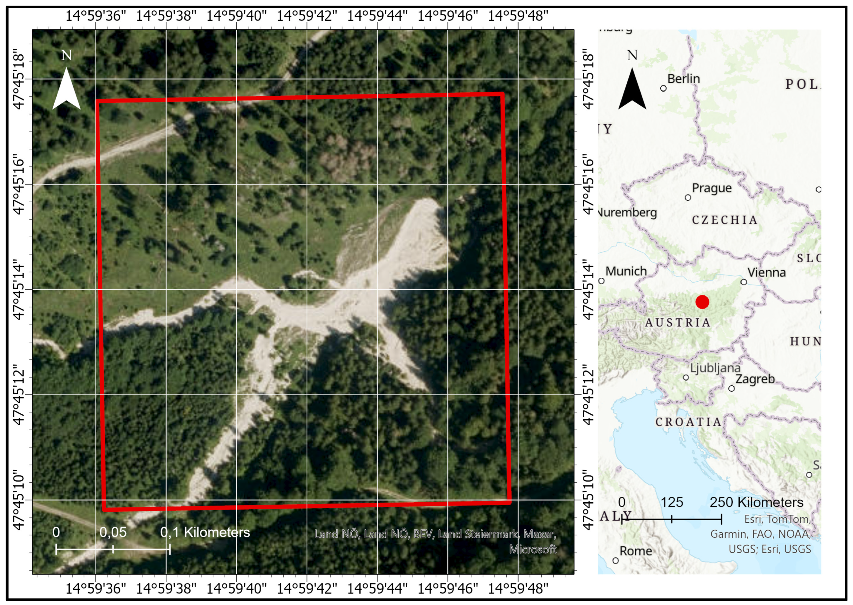
Figure 2.
Sample plots for the in-situ measurements.
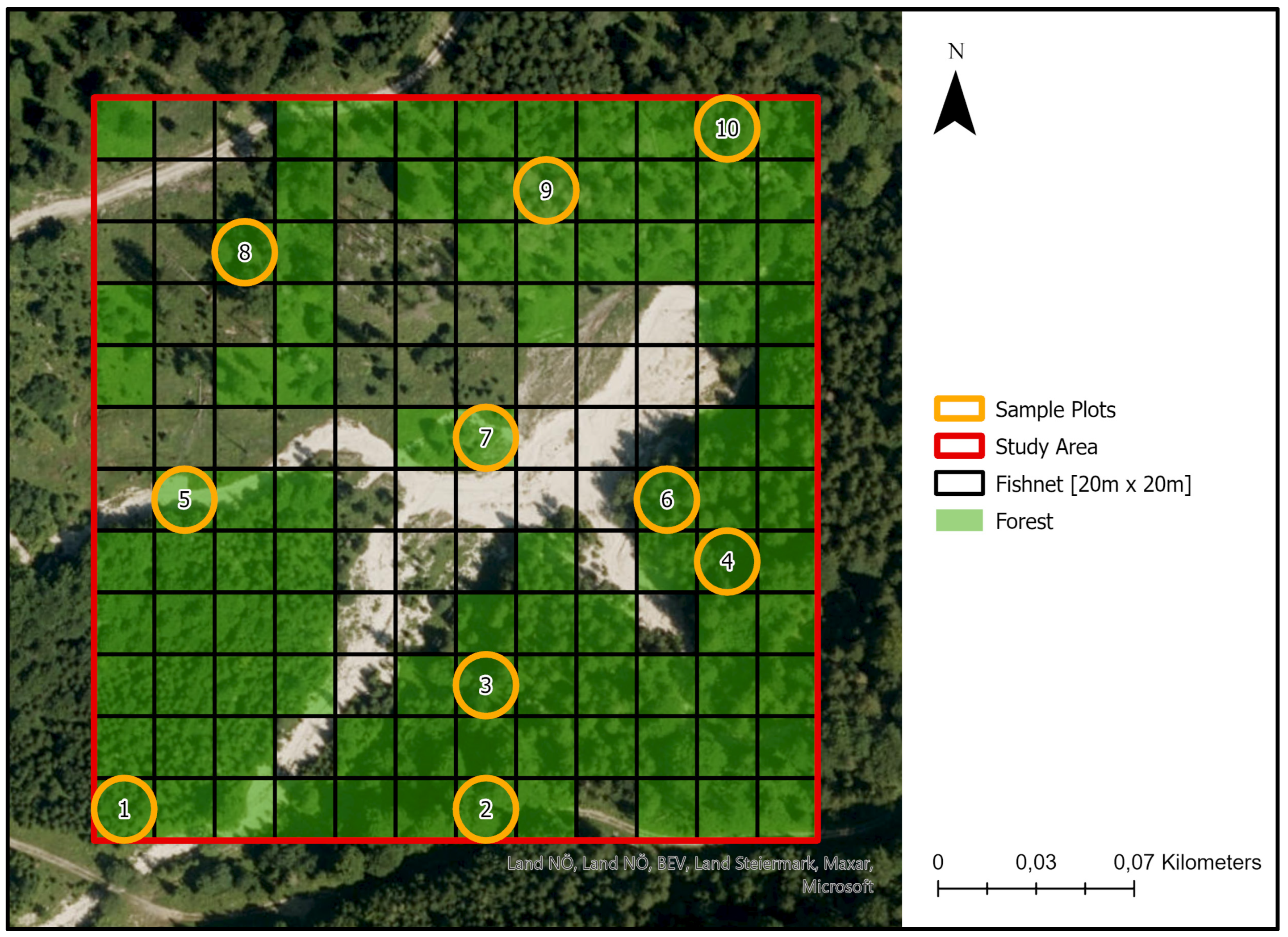
Figure 3.
Generated DSM and Orthomosaic with a resolution of 3 cm.
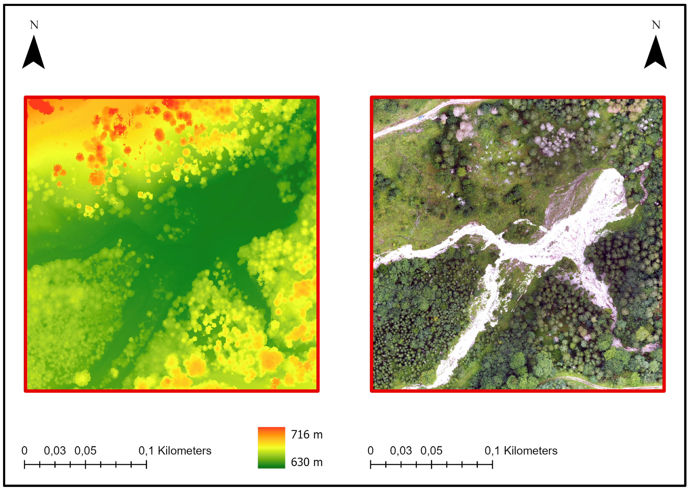
Figure 4.
NDVI indices with a resolution of 10 m.
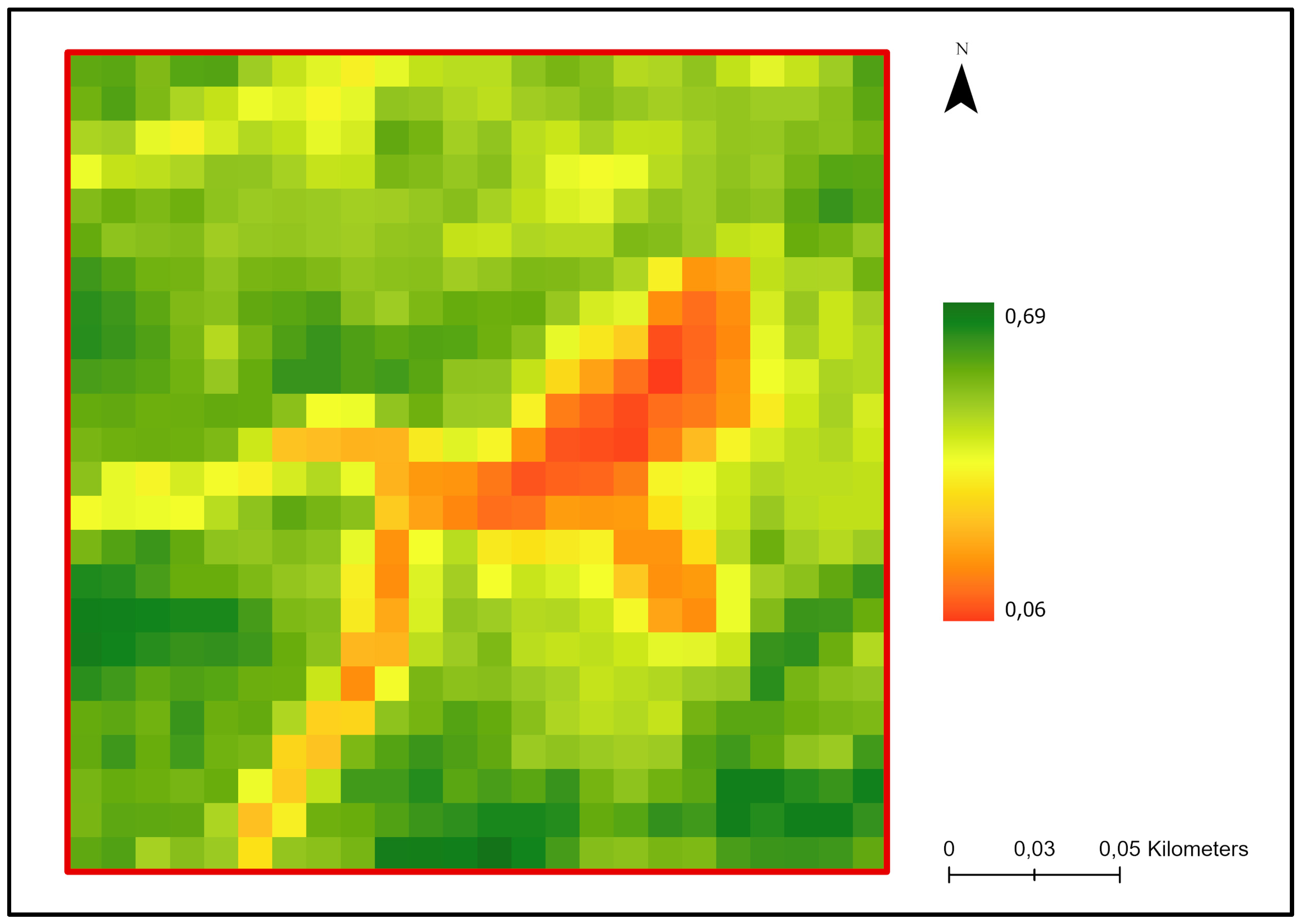
Figure 5.
Training samples.

Figure 6.
Reference dataset and validation points (blue) for the Image Classification Wizard.
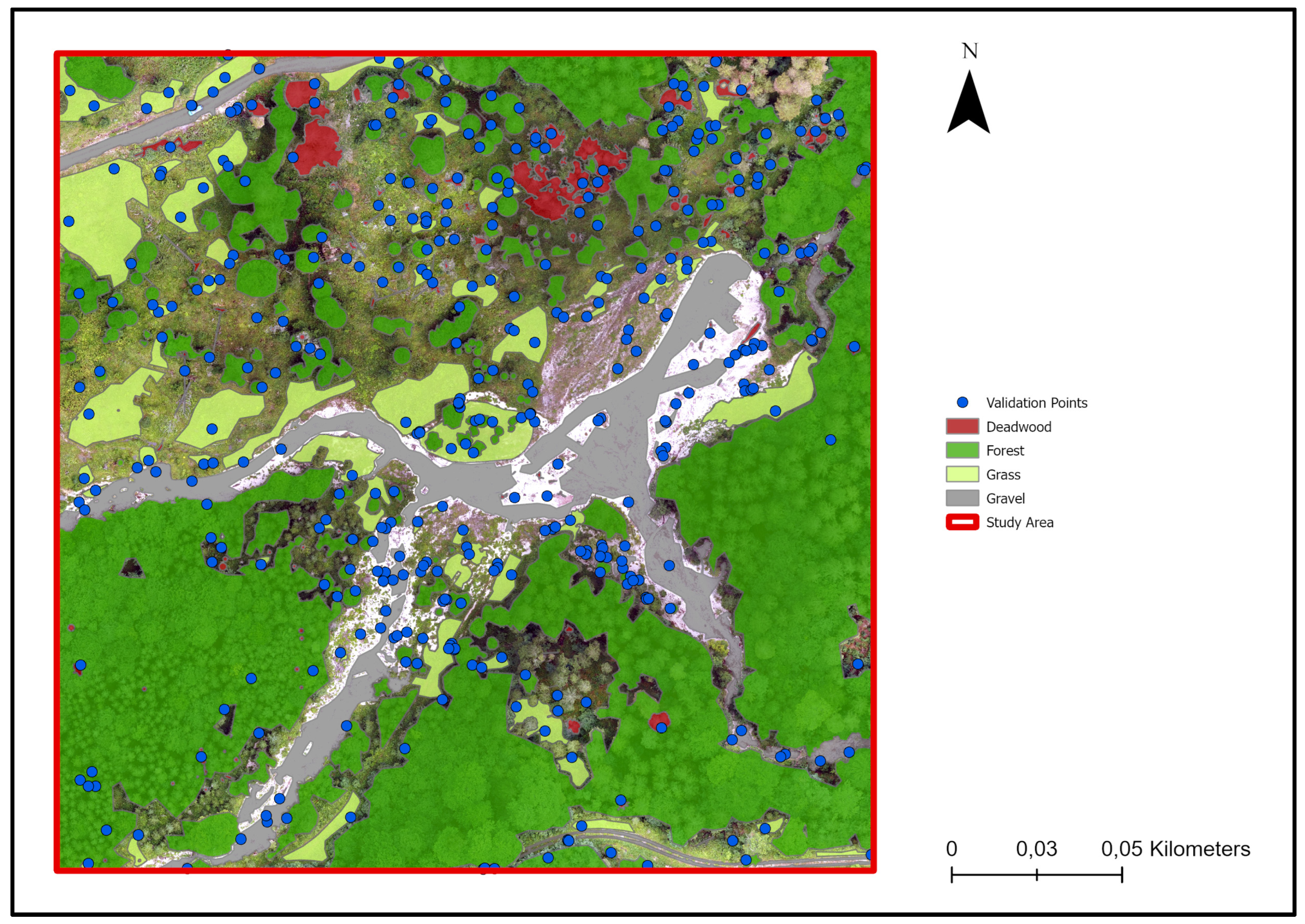
Table 1.
Volume correction according to Denzin.
| Tree species | Normal height (Hnormal) [m] | Volume correction per meter (Vcorr) [%] |
|---|---|---|
| European Spruce | 19 + 2*DBH [dm] | 4 |
| Common Beech | 25 | 3 |
| European Larch | 17 + 3*DBH [dm] | 5 |
Table 2.
Conversion factors for the Austrian forest.
| Conversion factor | Coniferous | Deciduous |
|---|---|---|
| m³ to t dm (stemwood) [tdmstem] | 0.38 | 0.54 |
| t dm stemwood to t dm whole tree [tdmtree] | 1.62 | 1.63 |
| t dm to t C [C] | 0.50 | 0.48 |
| t C to t CO2 [CO2] | 3.67 | 3.67 |
| summarized factor [factor] | 1.13 | 1.55 |
Table 3.
Composites with the corresponding datasets and bands.
| Composite | Datasets | Bands |
|---|---|---|
| 1 | orthomosaic | Red, Green, Blue, RGB-Alpha |
| 2 | Orthomosaic, NDVI | Red, Green, Blue, RGB-Alpha, NDVI indices |
| 3 | Orthomosaic, DSM | Red, Green, Blue, RGB-Alpha, DSM-Height |
| 4 | Orthomosaic, NDVI, DSM | Red, Green, Blue, RGB-Alpha, NDVI indices, DSM-Height |
Table 4.
AGB and carbon stock found in the field plots.
| Plot | Coniferous [m³] | Deciduous [m³] | AGB [m³] | Carbon stock [t CO2] |
|---|---|---|---|---|
| 1 | 5.367 | 0.259 | 5.626 | 6.464 |
| 2 | 0.165 | 7.484 | 7.649 | 11.791 |
| 3 | 4.999 | 1.626 | 6.625 | 8.169 |
| 4 | 5.119 | 2.245 | 7.364 | 9.264 |
| 5 | 0.303 | 1.667 | 1.970 | 2.926 |
| 6 | 18.541 | 1.030 | 19.571 | 22.541 |
| 7 | 0.704 | 0.009 | 0.713 | 0.810 |
| 8 | 11.446 | 0.844 | 12.290 | 14.238 |
| 9 | 2.228 | 0.046 | 2.274 | 2.588 |
| 10 | 0.672 | 0.301 | 0.973 | 1.225 |
Table 5.
Overall accuracies of the composites.
| Dataset/Composite | Overall accuracy [%] | Kappa value |
|---|---|---|
| Orthomosaic | 74.0 | 0.64 |
| Orthomosaic, NDVI | 76.3 | 0.68 |
| Orthomosaic, DSM | 80.0 | 0.73 |
| Orthomosaic, NDVI, DSM | 80.8 | 0.74 |
Table 6.
Confusion Matrix of the classification dataset.
| Class | Gravel | Deadw. | Grass | Forest | Total | U-Acc. | Kappa |
|---|---|---|---|---|---|---|---|
| Gravel | 93 | 12 | 1 | 0 | 106 | 88% | |
| Deadw. | 6 | 81 | 0 | 2 | 89 | 91% | |
| Grass | 1 | 7 | 87 | 36 | 131 | 66% | |
| Forest | 0 | 0 | 12 | 62 | 74 | 84% | |
| Total | 100 | 100 | 100 | 100 | 400 | ||
| P-Acc. | 93% | 81% | 87% | 62% | 80.8% | ||
| Kappa | 0.74 |
Table 7.
Carbon stock estimates and estimation errors.
| Plot | Carbon stock estimated [t of CO2] | Estimation error [t of CO2] |
|---|---|---|
| 1 | 11.344 | 4.880 |
| 2 | 11.409 | -0.38 |
| 3 | 10.745 | 2.58 |
| 4 | 11.609 | 2.34 |
| 5 | 3.886 | 0.96 |
| 6 | 11.513 | -11.03 |
| 7 | 0.238 | -0.57 |
| 8 | 8.213 | -6.03 |
| 9 | 5.403 | 2.82 |
| 10 | 4.826 | 3.60 |
Table 8.
Expenses (06/2024).
| Tool/Software | Period | MSRP/Cost |
|---|---|---|
| DJI Mavic Mini [76] | One-time | 399 € |
| Nikon Forestry Pro II [77] | One-time | 499 € |
| Tree caliper | One-Time | Approx. 100 € |
| ESRI ArcGIS Pro Advanced – NGO [78] | Annually | 220 € |
| Agisoft Metashape [72] | 30-day trial / One-time | 0 $ / 3,499 $ |
| Sentinel 2 datasets | One-time | 0 € |
Disclaimer/Publisher’s Note: The statements, opinions and data contained in all publications are solely those of the individual author(s) and contributor(s) and not of MDPI and/or the editor(s). MDPI and/or the editor(s) disclaim responsibility for any injury to people or property resulting from any ideas, methods, instructions or products referred to in the content. |
© 2024 by the authors. Licensee MDPI, Basel, Switzerland. This article is an open access article distributed under the terms and conditions of the Creative Commons Attribution (CC BY) license (https://creativecommons.org/licenses/by/4.0/).
Copyright: This open access article is published under a Creative Commons CC BY 4.0 license, which permit the free download, distribution, and reuse, provided that the author and preprint are cited in any reuse.


