Submitted:
04 September 2024
Posted:
09 September 2024
You are already at the latest version
Abstract
High-wind structures were identified in the Cross-Calibrated Multi-Platform (CCMP) ocean wind vector reanalysis for comparison with winds measured by satellite radiometers and synthetical aperture radar (SAR) instruments from February to October 2023. The comparison aims to evaluate bias, uncertainty, and spatial correlations with the goal of enhancing the accuracy of ocean wind datasets during tropical cyclones (TCs). In 10°longitude×10°latitude blocks, each containing a TC, Soil Moisture Active Passive (SMAP) and Advanced Microwave Scanning Radiometer 2 (AMSR2) winds are 6.5% and 4.8% higher than CCMP, while Advanced Scatterometer (ASCATB) is 0.8% lower. For extratropical cyclones, AMSR2 and SMAP also show stronger winds with a 5% difference, and ASCATB is about 0.3% weaker compared to CCMP. The comparison between SAR and CCMP for TC winds, sampled at the locations and time frames of SAR tiles, indicates that SAR winds around TCs are about 9% higher than CCMP winds. Using empirically defined TC structural indices, we find that the TCs observed by CCMP are shifted in locations and lack a compact core region. A Random Forest (RF) regressor was applied to TCs in CCMP with corresponding SAR observations, nearly correcting the full magnitude of low bias in CCMP statistically, with a 15m/s correction in the core region. The hierarchy of importance among the predictors is as follows: CCMP wind speed (62%), distance of SAR pixels to the eye region (21%) and eye center (7%), and distance of CCMP pixels to the eye region (5%) and eye center.
Keywords:
CCMP
; SAR
; radiometers
; ocean winds
; mean percent differences
; Random Forest (RF) regressor
1. Introduction
Accurate and continuous ocean surface wind data at regular grids spanning a large domain are highly useful, especially for coastal cities. Such datasets are particularly crucial for mitigating losses associated with tropical cyclones (TCs), which are among the most dreaded natural disasters [Woodruff, Irish, and Camargo, 2013; Chan et al., 2024], as well as non-TC severe storms [Kong et al., 2020; Lai et al, 2024; Lan et al., 2024] which are usually accompanied by strong winds. In Hong Kong, a No. 8 wind signal is hoisted when a sustained wind speed is within the range of 63-117 km/h (17.5-32.5 m/s), at which point the entire city is shut down, leading to billions of economic losses. The horizontal structure of ocean surface winds for TCs is critical to the decision-making regarding whether a No. 8 wind signal should be enforced.
However, ocean surface wind observations suffer poor spatial coverage, intermittent temporal frequency, and low accuracy under high wind conditions [e.g., Escobar and Alvarez1, 2023; Atlas et al., 2011]. As TCs are associated with strong winds, immense cloud coverage, and heavy precipitation, measurement of ocean surface winds within TCs are extreme difficult using either ground-based or space-borne techniques.
Satellite measured winds are valuable, although their coverage is generally limited. A wide range of satellite measurements, including those from radiometers and scatterometers such as the Advanced Microwave Scanning Radiometer-2 (AMSR2) [Alsweiss et al., 2021], the Soil Moisture Active Passive (SMAP) [Meissner et al., 2017], the advanced scatterometer (ASCAT) on the meteorological operational (MetOp) platform [Figa-Saldaña et al., 2002], and the Cyclone Global Navigation Satellite System (CYGNSS) [Ricciardulli et al., 2021], as well as various Synthetic Aperture Radar (SAR) instruments (Radarsat-2, the RADARSAT Constellation Mission or RCM, and Sentinel-1) [Kroupnik et al., 2021; Badger et al., 2018], are available in regions affected by TCs. Additionally, buoy measurements that rely on wind sensors installed on moored ocean floaters [e.g., Schlundt et al., 2020] complement these satellite datasets.
Global ocean wind vector data reanalysis datasets, such as the Cross-Calibrated Multiplatform (CCMP) ocean winds, were developed to provide global coverage on regular spatial grids and time intervals through data fusion techniques [Atlas et al., 2011; Mears et al., 2019]. Other notable reanalysis datasets include the ECMWF v5 Reanalysis (ERA5), the National Centers for Environmental Prediction (NCEP) Reanalysis, Modern-Era Retrospective Analysis for Research and Applications (MERRA-2), and Japanese 55-year Reanalysis, all of which have an ocean wind product. However, these wind datasets typically exhibit a low bias compared to the measurements obtained from satellites, aircraft or ground-based instruments [Wallcraft et al., 2009; Pescio et al., 2021]. In contrast, CCMP winds demonstrate a significantly better ability in capturing strong winds compared to other reanalysis datasets, valuable for studying high-wind structures.
In this paper, we will compare CCMP with SAR and radiometer measured ocean wind speeds under high-wind conditions from February to October in 2023 and develop a machine learning (ML) model for reconstructing the high winds in the core of the TCs. The ML model will reproduce ocean wind speeds on the same grids as CCMP. The modeled wind speeds should be drawn closer to SAR, since the latter was used as the true state.
2. Datasets
2.1. CCMP
The CCMP ocean surface wind data set was developed using variational methods to blend satellite winds, in situ data, and numerical weather prediction to create a gap-free gridded wind estimate every 6 hours. The Remote Sensing Systems group (RSS) produced versions 2.0, 2.0-2.1 NRT, and 3.0-3.1 of CCMP data. Non-NRT data availability has a 3-month latency due to delayed in situ measurements, while CCMP-NRT uses NCEP analysis winds as the background winds and has a one-day latency. CCMP 3.0 shows better agreement with independent buoy winds, especially for higher winds (>10 m/s) compared to v2.0 [Wang et al., 2023]. However, even the latest CCMP versions are accurate only at low to moderate wind speeds (<15 m/s) but tend to underestimate high winds [Mears et al., 2022].
Later on, we will discover that even though the CCMP dataset incorporated data from radiometers such as AMSR2 and ASCATB [Mears et al., 2019], the reanalysis and the individual datasets still display significant discrepancies in representing TCs. To assess these discrepancies, comparisons between CCMP and these datasets are conducted before attempting to improve CCMP during TC events. The study utilizes v2.1 NRT CCMP data.
2.2. Spaceborne Sensors for Wind Measurements
Imaging radiometers retrieve near-surface wind speed (but generally not direction) over the ice-free oceans by evaluating changes in microwave radiance caused by changes in the emission and scattering properties of the ocean surface as wind increases [Wentz, 1997; Meissner et al., 2017]. Specific microwave wavelengths are sensitive to a feature known as Bragg scattering, which is a characteristic of centimeter-scale ocean surface waves known as capillary waves. Capillary waves are directly influenced by changes in near-surface winds, which enable specially tuned airborne radars to observe these changes.
In contrast to passive microwave radiometers, the active radar system can combine measurements from different azimuth angles to derive the approximate direction of the wind. Due to the dependence of Bragg scattering on the azimuth angles, these types of radars are specifically categorized as scatterometers.
The SAR concept combines acquisitions from a shorter antenna to simulate a larger antenna, providing higher resolution data. SAR uses X, C, and L bands to detect ocean winds. SAR looks perpendicular to the spacecraft path at one azimuth angle to achieve high resolution in the azimuth direction by synthesizing a long array through platform movement. Ground-range resolution depends on the bandwidth of the transmitted signal and the imaging angle. A larger bandwidth improves range resolution.
For the sensors addressed below, their highest-level products exhibit spatial resolution of 0.5-1 km for SAR level-2 data and roughly 25 km (0.25°×0.25°) for level-3 imaging radiometers’ data.
2.2.1. AMSR2 (2012-Now)
The AMSR2 instrument aboard the JAXA GCOM-W1 satellite provides data on global precipitation, ocean wind speed, water vapor, sea ice concentration, brightness temperature, and soil moisture. JAXA AMSR Science Team and RSS generate their respective AMSR2 products, including the ocean wind speed with spatial resolution ranging from 15-35 km for low-frequency and 3-7 km for medium-frequency bands. This study utilized RSS-processed level-3 all-weather wind speed (AWS) data using the low-frequency band. The AMSR2 AWS product uses a statistical-based algorithm with multivariate regression and empirical corrections, covering various wind speed regimes in the training dataset. It has the capability to estimate wind speeds in areas of the storms that were usually flagged due to high rain contamination. AMSR2 AWS performance is comparable to SMAP, offering high sensitivity at extreme winds despite lower resolution [Alsweiss et al., 2021; Ricciardulli et al., 2023].
2.2.2. SMAP (2015-Now)
SMAP measures Earth's soil moisture and freeze-and-thaw state using L-band radiometer and radar instruments with a rotating 6-m mesh reflector antenna [Entekhabi et al., 2010]. RSS utilizes the L-band radiometer to retrieve surface wind speeds at 10 meters above the sea surface, providing wind speeds up to 70 m/s [Yueh et al., 2016]. However, the sensors have a slightly lower spatial resolution (~40 km). SMAP's long wavelengths enable wind speed measurements in intense storms without rain interference, especially at high wind speeds (>15 m/s), but the radiometer noise remains significant [Meissner et al., 2017].
2.2.3. ASCATB & C (2012&2018-Now)
ASCAT winds products (25 km effective resolution sampled at 12.5 km) are retrieved from the scatterometer instrument on EUMETSAT Metop polar-orbiting satellites. The radar instrument measures backscatter to determine both ocean surface wind speed and direction [Anderson et al., 2013; Figa-Saldaña et al 2002]. ASCAT operates at a C-band frequency (5.255 GHz) providing day- and night-time measurements unaffected by cloud cover with two 500 km parallel swaths. Originally planned to operate sequentially, ASCATB and C now operate simultaneously, with Metop-A decommissioned in November 2021. RSS's ASCATB and ASCATC ocean winds exhibit similar quality, leading to the selection of ASCATB for this study.
2.2.4. CYGNSS (2016-Now)
The CYGNSS mission employs eight micro-satellites to measure ocean wind speeds using a constellation of passive sensors that receive L-band GPS pulses. The Delay Doppler Mapping Instrument (DDMI) on each satellite utilizes scattered GPS signals to retrieve winds over a 1480 km swath with a 25 km spatial resolution. With an orbital inclination of approximately 35°, CYGNSS revisits locations on average every seven hours and every three hours at the median. This setup allows CYGNSS to measure ocean surface winds between 38°N and 38°S latitude, the critical latitude band for TC activity [Ruf et al., 2016; Ruf and Balasubramaniam, 2019].
2.2.5. RCM1-3/Radarsat-2 (2019/2007-Now)
Launched in June 2019, RADARSAT Constellation Mission (RCM) trio satellites aim to ensure continuity of operational SAR imagery for RADARSAT-2 users, as well drawing from the constellation approach to enable new applications [Kroupnik et al., 2021; Cote et al., 2021]. There are three identical satellites on one set of polar sun-synchronous orbits. Each of the spacecraft consists of a bus and a C-band SAR payload centered at 5.405 GHz. Using three satellites means the RCM can revisit and image the same location much more often, and in our case the RCM trio can capture TCs much more frequently than Sentinel-1, serving as the primary source of SAR measurements of TCs.
The RADARSAT-2 is the predecessor of the RCM with a very similar SAR payload. Both Radarsat-2 and RCM can achieve spatial resolution of 1m×4m. The wind product grid size is 0.5 km.
2.2.6. Sentinel A/B-1 (2014/2016-Now)
The Sentinel-1 mission is a European radar observatory for the Copernicus initiative by the European Space Agency (ESA). It carries a C-band SAR with a frequency of 5.405 GHz, featuring a fast-scanning antenna in elevation and azimuth. Sentinel-1 operates in four imaging modes with different resolutions (5-100m) and coverage up to 250-400 km per image tile. The level-2 ocean wind field is a ground range gridded estimate of the surface wind speed and direction at 10 m above the surface with 1 km resolution.
2.2.7. Orbiting and Local Time Coverages
AMSR2, SMAP, and ASCAT are polar orbiting instruments with approximately fixed daily local time coverages when crossing the equator, although these times differ significantly between them, as shown in Figure 1. In contrast, CYGNSS has a low inclination angle, resulting in varying local time coverage throughout the day, as illustrated in Figure 2. AMSR2 has local times at descending/ascending nodes (LTDN/LTAN) at 1:30 am/1:30 pm with a swath of 1400-1600 km; SMAP at 6 am/6 pm with a swath of approximately 1000 km; and ASCATB at 10 am/10 pm with two swaths of 500 km each. Both RCM3 and Sentinel-1 are in a sun-synchronous orbit with LTDN/LTAN at 6 am/6 pm. The Sentinel-1 swath (250-400 km depending on the operational mode) is smaller than that of RCM3 (500-600 km). Figure 1 and Figure 2 illustrate the challenge of finding time coincidences between these satellites, indicating near-zero opportunities for simultaneous observations of the same TC event. We did find a small number of coincidences between the SAR measurements and SMAP (not shown).
3. Results
3.1. Radiometer Related Comparisons
3.1.1. Global Comparisons between Radiometers and CCMP
In our first set of comparisons, we search coincident pairs between CCMP and ASMR2, SMAP, CYGNSS, or ASCATB respectively within 0.5-hour time windows throughout February-October 2023, on pixels sized at 0.25˚×0.25˚ grid over the global domain. January and December are excluded because no TCs are recorded in these months in 2023. Note that in this set of comparisons, we used the original 6-hourly CCMP data. For each pair of such coincident maps, the mean percent difference (MPD) is defined as: , where Vobs and VCCMP are wind speeds of the satellite observation and the CCMP reanalysis, respectively, and M is the total number of the coincident pixels for a given pair of maps. The global comparison would mingle high and low wind conditions that may show qualitatively different results. The standard deviation (STD) is calculated for the percent differences of the pixel-pairs for a given 0.5-hourly window. The standard error of the mean (SEM) is STD/sqrt(M) describing whether the MPD is statistically significant.
Histograms displaying the MPDs, STDs, SEMs, and correlation coefficients for the global-wise 0.5-hourly coincident map pairs are presented in Figure 3. In Figure 3a, it is evident that the distributions of the MPD histograms for all four instruments (versus CCMP) are similar in shape and peak values. This implies that there are no significant differences in the total coincident numbers of pairs (with CCMP) among them, all being close to 1000. The analysis reveals that, on average, all four instruments exhibit lower wind speeds when compared to CCMP, with CYGNSS showing the lowest winds whereas ASCATB more closely resembling CCMP. The median MPD relative to CCMP does not exceed 3%, and the spread of MPDs in the histograms, indicated by the STD of the MPDs across the global-hourly map pairs (in Figure 3a), falls between 4% and 12% for different data sets. This spread is sufficiently small to indicate a relatively consistent MPD across the hourly maps.
The STDs of the pixel-by-pixel percent differences (Figure 3b) in each global-hourly map pair ranges from 20% to 33%, far exceeding the MPD. This indicates substantial variability in wind differences among data points within a single map, as they encompass different wind features. The STDs for SMAP and CYGNSS are generally larger, implying a noisier map, with CYGNSS consistently exhibiting higher noise levels with a narrow spread in its histogram. In contrast, AMSR2 and ASCATB exhibit similar distributions for the STDs, both indicating a lower level of noise compared to SMAP and CYGNSS. The histograms of the SEMs in Figure 3c range between 0.2% and 0.3%, indicating a statistically reliable MPD (i.e., bias) shown in Figure 3a.
The histograms illustrating the spatial correlation coefficients between pairs of maps, shown in Figure 3d, exhibit peaks at 0.8-0.9 with a small spread of <0.3, indicating a strong correlation global-wise between the radiometer and CCMP winds. The histograms for AMSR2 and ASCATB display highest peak values, but their distributions for lower correlation coefficients differ. The ASCATB distribution has a much thicker tail, with 19% pairs having a correlation lower than 0.6 and a STD of 0.3. This means that structural-wise ASCATB has more outliers. The correlation of CYGNSS with CCMP is distinctly lower compared to the other three datasets, but it has a low spread (STD<0.1), with all pairs having correlations greater than 0.6.
Next, we compare the statistics between the 6-hourly CCMP data and the 0.5-hourly interpolated CCMP data. This comparison aims to validate the interpolation approach, as having CCMP data on more timeframes is crucial for achieving improved coincidences when TCs are detected by radiometers or SAR instruments. Figure 4 shows the results of comparisons between the SMAP and CCMP using 6-hourly versus 0.5-hourly CCMP data. After interpolating the CCMP winds to 0.5-hour intervals, the histograms of the MPDs, STDs, SEMs, and correlation coefficients exhibit strikingly similar distributions compared to the 6-hourly results. However, a small decrease in bias (Figure 4a) is observed post-interpolation, changing from -1.6% to nearly zero. This shift is attributed to a more pronounced positive wing emerging, although the peak still resides slightly on the negative side. This shift may be attributed to the increased capture of TCs with the availability of data on more frequent timeframes.
3.1.2. Identify High-Wind Structures within 10˚×10˚Blocks
Our primary focus is to address the high-wind structures over the oceans, as they are of significant concern. However, before proceeding with the main analysis, in Figure 5 we present a CCMP map showcasing complete global coverage to illustrate the prevalence and distribution of high-wind features in a snapshot of the global wind map. Figure 5 highlights not only the presence of TCs in the low-latitude region but also the extensive, large-scale high-wind structures along the zonal bands in the middle to high latitudes. In Figure 5, it is evident that both Saola and Haikui were observed near the coast of China. The two TCs are many times smaller in size compared to the larger-scale high-wind structures found in the middle to high latitude regions. These mid-high latitude structures are notably more prevalent in the Southern Hemisphere (SH), coinciding with the dominant coverage of oceans in that region. The shape of the high wind features (in Figure 5) resembles the hooked tail structure described in Browning [2004]. These extratropical cyclones (ETCs) typically last 2 to 5 days, have a diameter of 1000-2500 km, and exhibit wind speeds of 35 m/s or greater, comparable to a TC, in rare cases reaching 60 m/s [Pichugin et al., 2023].
To focus solely on the high-wind structures captured by the several radiometer datasets used above, we systematically search a global map in small blocks. In the context of this study, we consider a block (sized 10˚×10˚) containing a high-wind structure if it has 30% data coverage, 30% of data with wind speeds exceeding 14 m/s, and 5% data with wind speeds exceeding 26 m/s. Throughout the subsequent discussion, we utilize 2 m/s as an incremental step, beginning from zero. The threshold of 14 m/s represents approximately the lower limit of a tropical depression, while 26 m/s corresponds to the median wind speed of a tropical storm. These thresholds are generally set lower due to the challenges associated with satellite wind retrieval within TCs, which often result in a bias towards lower wind speeds. For instance, in SAR wind retrievals, the saturation of the C-band Geophysical Model Function (GMF) would create such a low bias [Hersbach et al., 2007].
Each valid block is analysed using the MPD (as defined) to present its fundamental statistical characteristics, followed by the generation of histograms depicting the distribution of MPDs across all blocks. The segmentation of pixel pairs into distinct block-wise statistical sets is to assess both pixel-level consistency within a single block and the overall agreement at the block level simultaneously.
As describe above, we have linearly interpolated the CCMP winds onto 0.5-hour intervals to enhance the data set, increasing the likelihood of coincidences with the satellite high-wind blocks. This approach is based on the understanding that in many cases a TC does not significantly change its morphology within 6 hours.
3.1.3. High-Wind Structure Comparisons between Radiometers and CCMP
The histograms of statistics in Figure 6 (and later in Figure 10) differ from those in Figure 3 by being block-wise rather than global-wise, focusing on low-latitude and mid-latitude regions respectively with a division at 35˚N/S. Features identified within the 35˚S-35˚N range are predominantly TCs, although some lose their circular shape near the 35˚N/S boundary.
Results for CYGNSS are not shown as no high-wind structures were detected during the specified period. Additionally, the number of high-wind structures identified in the ASCATB data is also notably lower compared to SMAP and AMSR2, attributed to the systematically lower winds measured, particularly in the high-wind scenario [Ricciardulli et al., 2021].
3.1.3.1. TCs
The median MPDs in Figure 6a show that under TC conditions, SMAP and AMSR2 wind speeds are 6.5% and 4.8% higher than CCMP respectively, while ASCATB is slightly lower than CCMP at -0.8%. The spreads (in STDs) among blocks are 5% for AMSR2, 14% for SMAP, and 10% for ASCATB. AMSR2 and SMAP exhibits the least and largest variability across blocks.
In Figure 6b, the STD of the percent differences within a block ranges from 17% to 20%, which exceed the MPDs by far indicating considerable variability across pixels within each block for all three radiometers. The spread of the histograms ranges from 5% to 15%, reflecting substantial variability across blocks, again with SMAP exhibiting the widest range. Figure 6c shows that the SEM remains 10 times lower than the MPD in all cases, pointing to statistically significant MPDs.
The spatial correlation, as shown in Figure 6d, remains generally strong (0.8-0.9 with minimal variation). However, it is systematically weaker and exhibits larger spread than the correlations shown in global comparisons, as the previously stronger correlation is mainly contributed by large-scale structures whereas a smaller domain containing a TC generally exhibits larger variabilities. Figure 6d indicates that about 7-18% of block-pairs exhibit poor correlation (< 0.6), in which AMSR2 shows notable worse agreement with CCMP when TCs are present.
Figure 7, Figure 8 and Figure 9 display five pairs of maps, with each set chosen by the highest spatial correlation coefficients, extensively showcasing the ability of AMSR2, SMAP, and ASCATB to capture TC structures. Figure 7 indicates that AMSR2 shows consistently higher TC wind speeds than CCMP, supporting the findings in Figure 6a. What is noteworthy is that AMSR2 is prone to capturing filament structures not visible in CCMP or other radiometer datasets, suggesting that it may be better at capturing TCs’ small scale structures. Additionally, CCMP maps often capture distinct TC eye centers with low winds (< 8 m/s), while AMSR2 does not exhibit distinct eye centers in its eye region. Similarly, SMAP measured winds are systematically higher than CCMP, but the morphology of TCs exhibit better resemblance to CCMP compared to other data sets. As supported by Figure 6a, TC wind speeds in ASCATB are consistently lower than in CCMP, which may have led to the overall less organized TC structures in most of its maps. Also, neither SMAP nor ASCATB maps show distinct eye centers.
3.1.3.2. Extratropical Cyclones
Extratropical cyclones (ETCs) play a critical role in shaping daily weather fluctuations at middle and high latitudes, frequently leading to the occurrence of severe winds and waves [Browning, 2004; Ponce de León, 2015], storm surges, and intense precipitation [Pfahl et al., 2016], both at sea and along coastlines [Pitrugin et al., 2023]. Even though ETCs are not the main focus in this paper, we shall make parallel comparisons to evaluate how they are represented by the several data sets.
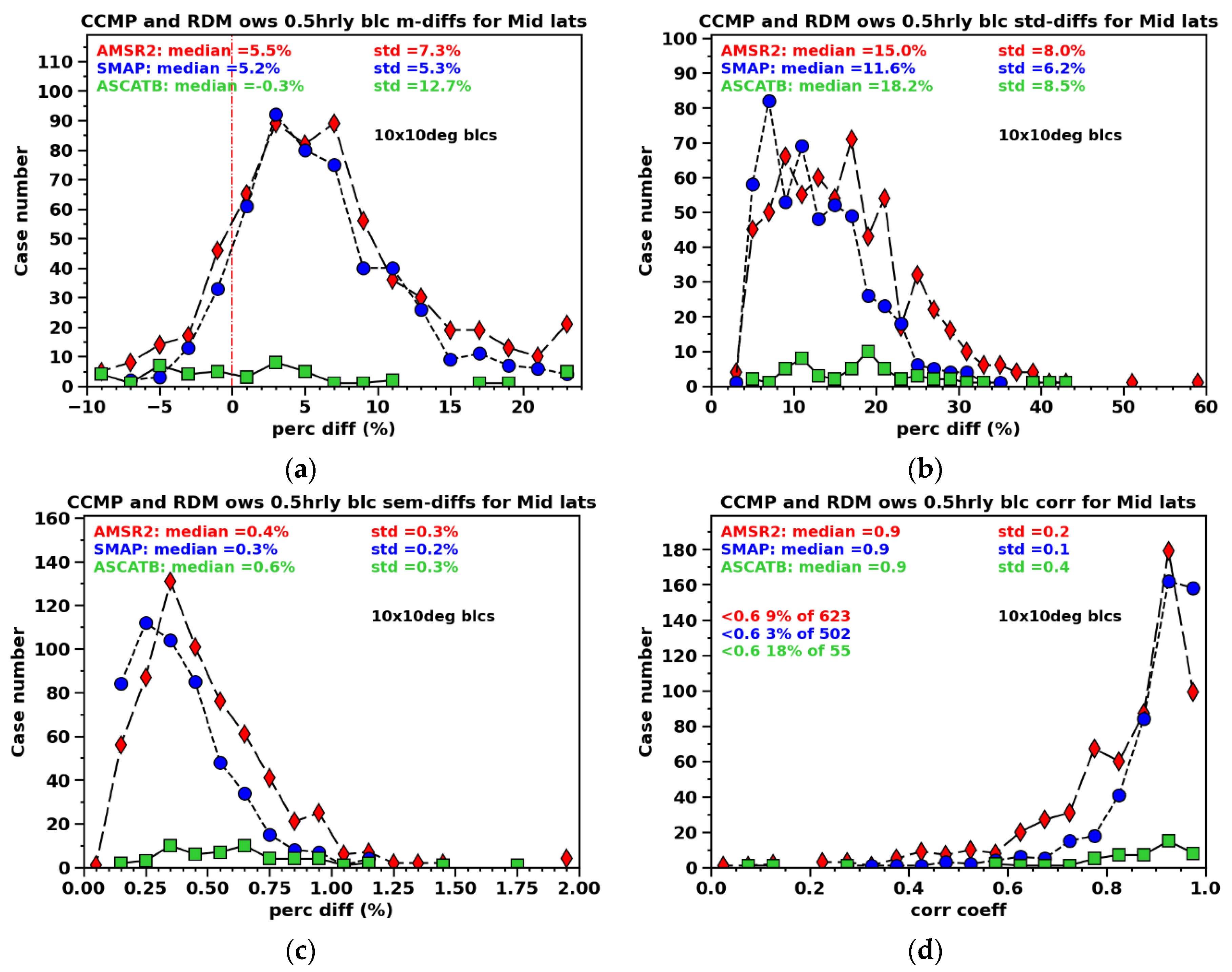
The statistical analysis for the ETC comparisons is presented in Figure 10, following a similar format to the TC analysis in Figure 6. The medians of MPDs of wind speeds for AMSR2 and SMAP (relative to CCMP) are approximately 5%, and both are statistically significant. These differences are slightly smaller but comparable to those observed in the TC analysis. Similarly, the median of MPDs for the ASCATB versus CCMP comparisons is -0.3%, mildly smaller than the -0.8% in the TC comparisons, and is smaller than the SEM at 0.6%, which points to a zero bias. To summarize, the overall agreement between the three data sets and CCMP is better for the ETCs.
In Figure 10b, the STD of the percent differences with CCMP across pixels within a specific block consistently points to lower variability in the mid-latitude region compared to the TC cases for SMAP and AMSR2, indicating a smaller degree of uncertainty for ETC cases. This would support a better agreement of radiometer winds with the CCMP in the extratropical region as high winds are present.
The spatial correlation for the ETC cases demonstrates greater consistency (than the TCs) among blocks for all data sets used, as illustrated in Figure 10d, with all median correlation coefficients reaching 0.9. The fractions of pairs with low correlation are slightly larger than in the global comparisons but generally very small, suggesting that in ETCs achieving agreement between radiometer winds and CCMP is not as challenging.
The ETC maps presented in Figure 11, Figure 12 and Figure 13 are characterized by larger scale structures with more irregular shapes relative to TCs, with some displaying co-existing low- and high-wind structures. Although the histograms (in Figure 10a) have shown that the MPDs of AMSR2 and SMAP are in the same direction, only the SMAP maps have shown dominantly higher wind speeds compared to CCMP, as shown in Figure 12. While the differences between the AMSR2 and CCMP maps are notably smaller. This mild discrepancy arises from the double-peak histogram in AMSR2 shown in Figure 10a, leading to a wider spread among blocks (7.3% for AMSR2 versus 5.3% for SMAP). Previously Figure 10b has also shown that AMSR2 exhibits a higher median STD (15% versus 12%) and also a larger variability among blocks (8% versus 6%). Both point to a mildly larger variability in AMSR2 in representing the ETCs than in SMAP. Despite the differences, the three datasets demonstrate overall similar effectiveness in capturing the morphology of ETCs. This differs from the TC comparisons, where AMSR2 and SMAP display filamentary or well-organized circular structures, distinguishing them from ASCATB.
Figure 10.
Same as Figure 6, except for the mid-high latitude region south of 35° S or north of 35° N.
Figure 10.
Same as Figure 6, except for the mid-high latitude region south of 35° S or north of 35° N.
3.2. SAR and CCMP Comparisons
3.2.1. TC Selections Captured by SAR
Except for Sentinel-1, other SAR data is not as readily available as the wind measurements from radiometers. Therefore, we utilize the TC data available from the NASA Satellite Oceanography and Climate Division (SOCD)’s website which the public has access to. The selected TC events include Mawar (May), Saola (September), and Koinu (October) in the west Pacific; Calvin (July), Hillary (August), and Dora (August) in the east Pacific; Franklin (August), Lee (September), and Nigel (September) in the Atlantic (ATL); Biparjoy (June) and Mocha (May) in the north Indian Ocean; and Freddy (February-March), Herman (March), and Ilsa (April) in the southern hemisphere (SH). These events spanned from February to October of 2023.
3.2.2. Basic Statistics
Statistics similar to the radiometer related comparisons are shown in Figure 14 for pairs of SAR versus CCMP coincidences, with both datasets interpolated onto a 0.125˚×0.125˚ grid using an averaging window of 0.25˚. The CCMP data is so resampled to produce smoother structures, enhancing the stability of structural indices calculated for TCs (see 3.2.3). Both data sets have a virtual spatial resolution of 0.25˚×0.25˚. Rather than using 10˚×10˚blocks, MPDs are calculated for individual SAR tiles collected in the SOCD TC website. CCMP is resampled based on the time and domain of the SAR tiles. Figure 15 presents a similar set of histograms to those shown in Figure 6, but uses a block size of 5°×5° instead of 10°×10°. This change is made because the SAR tiles are approximately 4° longitude by 5° latitude each, and we aim to examine the radiometer and SAR measured winds on the same platform.
In Figure 14 the median MPD between the SAR and CCMP winds across all tiles is 9%, and it is statistically significant based on a generally very small SEM (i.e., 0.68%). The spread among tiles reaches 12% indicating large variability across tiles. The median STD of the percent differences is 21% illustrating variability across pixels within a tile. Figure 15a shows that the median MPDs from CCMP for AMSR2 and SMAP are 8% and 12%, respectively, both of which are comparable to the SAR comparisons. While ASCATB has a MPD of -3.5%. In contrast to Figure 6a, Figure 15a displays generally magnified MPDs due to the domain being more compressed toward the core of TCs, resulting in greater variability between datasets. The levels of uncertainty, measured by standard deviations (STDs), are comparable between Figure 14 and Figure 15.
The median correlation between SAR tiles and CCMP data is 0.74, with 23% of pairs having a correlation lower than 0.6. Figure 15d shows that the median correlation coefficients for the radiometer-related comparisons within 5° × 5° blocks range from 0.6 to 0.8, similar to the levels observed in the SAR comparisons. In the AMSR2 versus CCMP comparisons, 45% of pairs exhibit low correlation coefficients, the highest among the datasets. Results from Figure 14 and Figure 15 suggest that incorporating the radiometers’ winds into CCMP did not significantly improve their agreement with CCMP compared to SAR winds in regions where TCs are present. Nevertheless, SMAP does appear to align better with CCMP across major aspects.
In line with earlier comparisons, Figure 16 shows the SAR and CCMP maps with the highest spatial correlations. All five pairs indicate dominantly stronger winds within the SAR-captured TCs. Notably, the SAR data reveals weaker winds in the surrounding regions, a feature that might also be present in the radiometer comparisons but not as clear. Despite its more than 10 times higher spatial resolution, SAR also does not consistently capture distinct low-wind eye centers, and this is not due to resampling onto a coarser grid.
3.2.3. TC Structural Indices
SAR employs a technique that involves the movement of the radar system and the integration of signals to achieve high spatial resolution, enabling it to resolve ocean winds at a resolution up to 1 km. This illustrates the detailed structure of a TC more effectively than radiometers.
In this study, without relying on more external data sources, we utilize empirically defined TC eye-center position, eye-region size, south-north and west-east asymmetries, and wind speed versus equivalent radius curves to characterize a TC. These specific indices are employed within the scope of this study to facilitate comparison between SAR and CCMP data.
The TC eye center is identified as the point where the minimum wind speed occurs within the core region characterized by high winds. To ensure a reliable result, a range of wind speed levels is used to define the high-wind region, spanning from vmax-10 to vmax (where vmax represents the maximum wind speed recorded by SAR or CCMP for a specific TC) in 2 m/s increments. From the identified centers at individual wind speed levels, the position with the lowest wind speed value is selected. This approach of utilizing multiple wind speed levels is necessary because, at a single level, the pixel distribution may exhibit significant asymmetry, potentially leading to inaccurate center determination.
The eye-region size, quantified by a collective set of pixels, are searched within a range of ±6 pixels (a total of 168 pixels) from the TC center in a rectangular domain along the longitudinal and latitudinal directions. If the wind speed of any of these pixels is 4 m/s (equivalent to two incremental levels) lower than the highest wind speed values in the neighbouring pixels, ideally in all radial directions, it is classified as an eye-region pixel. In most cases, however, examining all relevant pixels along both the longitudinal and latitudinal directions is sufficient.
Figure 17 demonstrates how the approach works by applying it to the pair of maps in Figure 16e. It is important to note that when TCs are in their weakening stages, in some cases CCMP tends to display a more elongated structure. As a result, there could be uncertainty in determining the eye center, as shown in Figure 17b. However, this is not expected to qualitatively impact the statistics of the comparison results.
Figure 18 showcases the equivalent radii comparisons of TC structures corresponding to the maps in Figure 16, relative to the respective TC centers. The wind speed levels span the range from 24-48m/s. In rare instances, such as in Figure 18c, the curves from CCMP and SAR overlap, but in most cases, CCMP does not capture high winds near the center. In addition, CCMP's equivalent radii for wind speeds that both data sets share point to a smaller TC, even though CCMP often portrays a less intense or seemingly degraded TC than it actually is.
The asymmetry in TC structures along the west-east and south-north axes (split at TC center) is quantified by calculating the fraction of pixels in the west or south of TC center (referred to as frac_w or frac_s) over the total number of pixels within a specific TC. The absolute difference between these fractions in SAR and CCMP datasets characterizes the magnitude of the asymmetry differences, whereas the sign of the difference is determined by multiplying each fraction by its deviation from 0.5. A negative sign indicates opposite asymmetry between SAR and CCMP TCs. A sequence of wind speed levels (ranging from 16-48 m/s with a 2m/s increment) are utilized to establish a more robust statistical set to correctly characterize the overall asymmetries of a given TC. These asymmetries briefly describe the wave-1 amplitudes and the phases revolving around the TC eye center.
Figure 19 shows the statistical moments of TC structural differences for all coincident pairs of the TC stances across different speed levels from February to October 2023. The histogram of eye-center distances indicates increasingly larger population at smaller values, with a peak around 10 km, indicating a general agreement between CCMP and SAR in identifying the eye centers over a large number of samples. The STD of differences is comparable with the median, both at 28 km, which indicates a significant level of variability across tiles.
The eye-region size measured in pixels is notably larger in CCMP compared to SAR, as shown in Figure 19b, with median values of 21 and 7 pixels (0.125°×0.125°), respectively. Both histograms show peaks at smaller eye regions, particularly in SAR, indicating that the majority of TCs in this analysis, which are likely not in a stage of severe degradation or at birth, have small eye regions.
The SAR equivalent radii are larger compared to CCMP, with a peak deviation at 15% in the histogram (shown in Figure 19c). Note that this difference is primarily observed in the range of relatively weak winds that CCMP is able to capture. As showcased in Figure 18 above, CCMP-observed TCs tend to be weaker, smaller, and lack a compact core region. The 25% spread suggests substantial variability between different TC instances.
Figure 19d presents the histograms of west-east and south-north asymmetries. When the asymmetries align between SAR and CCMP, the distribution approaches a zero difference with a median of 0.05, relatively to the maximum at 0.5. In 75% and 72% of cases, SAR and CCMP exhibit aligned asymmetries in either orientation. When the asymmetries do not agree, the absolute differences could reach up to 1.0. This occurs when all pixels are located in the west (frac_w=1.0) in SAR, while in CCMP, they are all in the east (frac_w=0.0). Notably, in only about 55% of cases do the SAR and CCMP TCs show simultaneous agreement in both west-east and south-north asymmetries, suggesting that SAR and CCMP wave-1 structures (relative to each TC eye center) do not align in phases nearly 50% of the time.
4. A machine Learning Model to Produce a Data Set Drawn Closer to SAR at TCs
As previously stated, our objective in validating the CCMP ocean winds is to investigate the feasibility of using artificial intelligence (AI) to develop a comparable data set to CCMP that can better represent high-wind structures. For our initial efforts, we have focused on SAR-measured winds to serve as our true state, as they provide the most detailed structure and the highest winds within a TC compared to other satellite data sets. We used CCMP and SAR coincident tile-pairs to train a machine learning model using the random forest (RF) regressor. This model is applied to generate wind fields in regions similar to SAR tiles where CCMP and SAR both contain a TC, aiming to unravel the relationship between CCMP and SAR winds.
The key hyperparameters of a RF model are: 1) the number-of-features selected for each split; 2) the sample size for each tree; 3) the minimum number of observations in a terminal node; 4) the number of trees in the forest; and 5) the criteria for splitting nodes. Using fewer features as predictors can lead to suboptimal tree performance but will lead to more diverse and less correlated trees allowing the model to better capture variables with moderate effects on the outcome. Nevertheless, the benefit of using the full set of features is to ensure that there is at least one strong variable among the candidates for splitting. This can enhance the overall performance of the model [Goldstein et al., 2011]. In this study, we adopted the latter approach by utilizing the regressor's default option to efficiently achieve a favourable outcome. This decision was based on the necessity of including the strongest predictor, which is the CCMP wind speed, for the model to function effectively. The effect of sample size aligns with that of the number of features, although it may have a lesser impact. The node size parameter sets the minimum number of observations in a terminal node, affecting tree depth and splits. Decreasing the node size results in deeper trees with increased splits, which can lead to longer runtimes for large sample sizes. The number of trees is also crucial, as more trees generally enhance model performance. However, the most substantial performance improvement typically occurs within the initial 100 trees [Probst and Boulesteix, 2017; Probst et al., 2019]. We have used a node size of one and a forest size of 100 trees in the model training.
The predictors chosen for this study include the CCMP wind speeds, distance from the eye center in longitude and latitude, i.e., Δlon and Δlat, Δlon and Δlat from the eye region, great-circle (GC) distance from TC eye center and eye region, for each of the two data sets respectively. Regarding the distance to the eye region, the following is true: when the pixels are among the eye-region pixels, the distance from the eye region will be zero, otherwise is the closest distance. These predictors are not entirely independent from each other. We came to use two of their subsets and then the full set of the predictors to build models, labelled Type-1, Type-2, and Type-1&2 models.
In the scatter plots comparing SAR data to model predictions (Figure 20), the error represents the mean absolute difference across all pairs of relevant ocean pixels, irrespective of tiles or timeframes. The bias is the mean difference over all pixels used; the RMSE is the square root of the sum of the bias squared and the variance. The correlation coefficient is derived from all pixel pairs in arbitrary order, without considering spatial or temporal dependencies. Accuracy is determined as 100 minus the median percentage absolute error. For individual percentage absolute errors, the SAR measurement serves as the denominator instead of the mean of SAR and CCMP, as SAR measurements are considered the true state. The total set of TCs named above is divided into training and testing sets at a 75% versus 25% split. When training the RF model with the training TC set, a similar 75% versus 25% split is applied, with 75% of pixel pairs used for model training.
The scatter plot for the training pairs (Figure 20a) shows zero bias, an absolute error and RMSE of less than 1.0 m/s, a correlation coefficient of 0.99, and 98% accuracy. These results demonstrate a strong agreement between the pairs in the training set, validating the effectiveness of the chosen predictors. However, overfitting is not ruled out, as hyperparameters were not tuned.
When the model is applied to the 25% of pairs not used in model training (still belong to the training TC-set), as shown in Figure 20b, the agreement is also remarkable, with a zero bias, 1-2m/s error, 0.96 of correlation, and 94% of accuracy. This high level of agreement can be attributed in part to the fact that these pairs originate from the same TCs used for training, despite not being part of the training set of pixel pairs. This consistency may be due to the continuity of the morphology of a specific TC across different time frames.
Upon testing the trained model on a separate set of TCs, which are the additional 25% of the TCs reserved for testing purposes, slight variations in results are observed between the three models trained with different predictor combinations. Figure 20c showcases the Type-1&2 model, with comprehensive details provided in Table 1 and Table 2. When utilizing all predictors in the Type-1&2 model, a bias of 0.3 m/s or lower, an absolute error close to 3 m/s, a correlation coefficient between 0.87-0.88, and an accuracy of 89% are achieved. The uncertainty in these results is twice as large as that seen in Figure 20a-b, which is expected.

Table 1.
Statistics of the test TCs using three types of RF models.
| Bias (m/s) | Error (m/s) | Rmse (m/s) | Corr | Accu | |
| Ty-1 | -0.18 | 2.94 | 4.28 | 0.87 | 89% |
| Ty-2 | -0.17 | 2.92 | 4.28 | 0.87 | 89% |
| Ty-1&2 | -0.32 | 2.86 | 4.16 | 0.88 | 89% |
Table 2.
Comparison of the relative importance of various predictors for the three RF models. The predictors include the great-circle distances to the TC's eye center and the eye region, as well as the corresponding distances in longitude and latitude.
Table 2.
Comparison of the relative importance of various predictors for the three RF models. The predictors include the great-circle distances to the TC's eye center and the eye region, as well as the corresponding distances in longitude and latitude.
| CCMP |
dis_ cen1 |
dis_ cen2 |
dis_ core1 |
dis-core2 | Δlon_ cen1 | Δlat_ cen1 | Δlon_ cen2 | Δlat_ cen2 | Δlon_ core1 | Δlat_ core1 | Δlon_ core2 | Δlat_ core2 | |
| Ty-1 | 0.63 | -- | -- | -- | -- | 0.03 | 0.03 | 0.04 | 0.03 | 0.07 | 0.06 | 0.04 | 0.08 |
| Ty-2 | 0.62 | 0.07 | 0.05 | 0.21 | 0.05 | -- | -- | -- | -- | -- | -- | -- | -- |
| Ty-1&2 | 0.61 | 0.05 | 0.04 | 0.20 | 0.03 | 0.01 | 0.01 | 0.01 | 0.01 | 0.01 | 0.01 | 0.01 | 0.01 |
Table 1 presents the statistical moments for all three models. While the results of all three models are notably similar, the Type-1&2 model exhibits the highest bias (-0.32 m/s relative to -0.18 m/s) indicating that the inclusion of all predictors may not necessarily lead to optimal results. Although these biases are minimal, they persist as low biases compared to SAR data, indicating substantial correction in CCMP data yet without a reversal in direction. Despite having a bias twice as large in Type-1&2 model, it marginally reduces the absolute error and RMSE. Notably, Type-2 outperforms Type-1 in terms of both bias and absolute error.
Once the RF models are being established, we refocus on our primary goal, which is to apply the model to individual tiles rather than a mixture of pixels. To evaluate the model's predictive performance on individual tiles, we apply the trained models to each TC tile individually and generate histograms for various statistical moments. The accuracy, bias, correlation, and STD are then presented in the four panels of Figure 21.
Notably, results from all three RF models have improved the "accuracy" compared to CCMP, reducing the percentage absolute error by 4%. The accuracy histograms of the RF model results exhibit a single peak significantly skewed towards higher values (around 90%), contrasting with the CCMP and SAR results that has a double-peak with a maximum at 85%.
The RF modeled results nearly fully corrected a low bias (2-3 m/s) in CCMP statistically, shown in Figure 21b. In fact, a slight overcorrection has resulted in a minimal high bias (0.02-0.07 m/s) that is not statistically significant. Yet, the histogram peaks for all three models are skewed towards the positive side. This small bias, not in line with Table 1, indicates that a different sampling method can slightly alter the bias direction.
Previously we have shown that TCs captured by CCMP and SAR generally exhibit drastically different morphologies. Their spatial correlation has a median coefficient of just 0.73 and a considerable spread across tiles statistically, shown in Figure 21c. In comparison, the results from the three models show much higher correlations consistently, with median values ranging from 0.85 to 0.87. This improvement is evident in the histograms, which consistently display a sharper single peak at higher correlation values, indicating a more robust alignment between the RF model predictions and the SAR data.
Figure 21d indicates the reduction of the STD by 15-20% (from 4.3 m/s to 3.7 m/s) in the results of all three RF models, suggesting that the difference between the RF modeled field and SAR becomes less fluctuating after applying the RF model to the CCMP fields, also suggesting a better agreement.
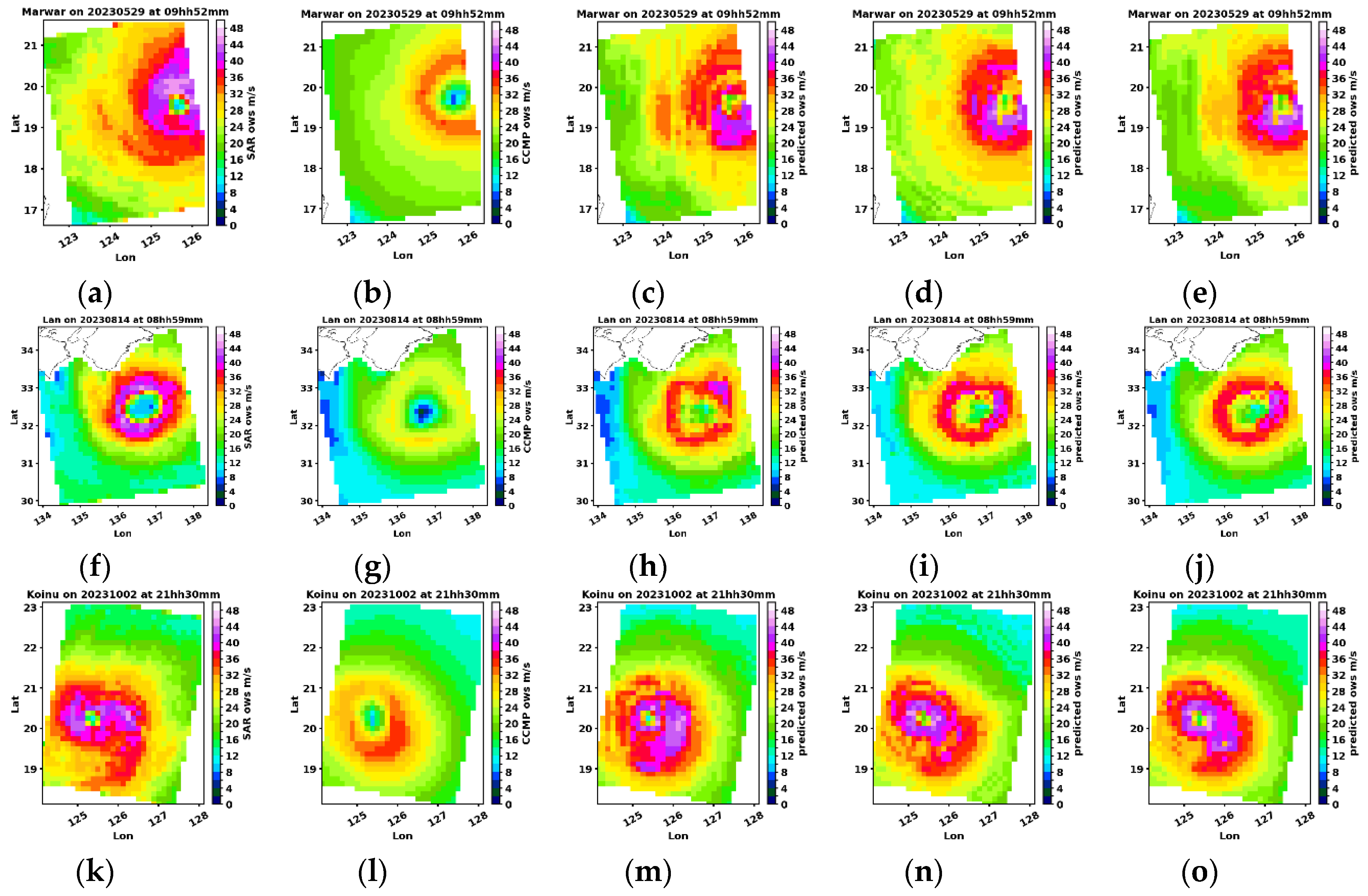
Figure 22 shows actual pairs of maps, in three rows, to demonstrate the results of the three models. Overall, in all three results, the wind magnitude and morphology are both drawn closer to the SAR retrieved winds. In many cases, the high wind region within the TC may still be weaker but the correction is substantial, reaching 10-15 m/s.
Upon closer examination of Figure 22, it is observed that in Type-1, where only Δlon and Δlat are used as predictors, the structure displays feature oriented along the longitudinal and latitudinal directions, which is particularly noticeable in column 3. On the contrary, in the Type-2 results (column 4), where the predictors include GC distance to the eye region and eye center, the structures tend to be circular in shape. These results align with the expectations based on the definitions of the predictors. Although Type-1 exhibits the generally less smooth structure, it effectively captures the thick filamentary structure with greater clarity. It is worth noting that Type-1&2 does not show better structure than the Type-1 or Type-2 even though it used all the predictors.
We next examine the relative importance of predictors in the RF model training, as listed in Table 2. Across all three RF models, the significance of CCMP wind speed stands out, as expected, ranging from 0.61 to 0.63. In Type-1, the importance is evenly distributed among its remaining predictors, with eye region-related predictors in both CCMP and SAR carrying more weight than eye center-related predictors. Type-2 shows a notable dominance of the distance-to-the-eye-region of the SAR tile at 0.21, exceeding each of the other predictors that share the remaining importance. For Type-1&2, the importance distribution resembles that of Type-2, with additional predictors each contributing a 0.01 fraction of importance.
What is shown in Table 2 indicates that the TC structural metrics in SAR served as significant predictors. But these metrics are unavailable when CCMP and SAR data are not paired. Nevertheless, we have come to understand that achieving high accuracy in the AI model's results will greatly benefit from incorporating certain structural metrics related to the SAR TCs as predictors. In future endeavours to establish an operational model, we will consider predicting TC's structural metrics as a prerequisite and then proceed to apply the models established above.
5. Summary
High-wind structures in the CCMP ocean wind reanalysis data set are compared with satellite radiometer-measured winds and SAR winds throughout February - October 2023 on hourly maps to assess bias, uncertainty, and spatial correlations. A global comparison is made between CCMP and radiometer-measured winds, and then ETCs and TCs within 10°×10° blocks are compared separately. The comparison between CCMP and SAR is focused on the TC episodes recorded in NOAA's SOCD. The ultimate goal is to utilize an AI approach to create a new data set in TC-affected regions to meet specific regional requirements, for which an attempt is made in this study but more work is required.
Irrespective of the high-wind structures, the global comparisons were conducted first, which suggest that all four instruments (AMSR2, SMAP, ASCATB, and CYGNSS) exhibit statistically lower wind speeds relative to CCMP, with CYGNSS showing the largest differences (-2.7%) whereas ASCATB (-0.6%) closely resembling CCMP. The coincidences were searched within 0.25°×0.25° grid and 0.5-hour intervals. The MPD histograms share very similar distributions among the four data sets with a narrow spread characterized by a STD falling between 4% and 12%, indicating a fairly consistent MPD across the hourly maps. The STDs of the pixel-by-pixel percent differences suggest that CYGNSS is the nosiest among the four data sets whereas SMAP noisiness varies more drastically over different hourly maps. The histograms of the spatial correlation coefficients peak at a high correlation of 0.8-0.9 with a small spread of less than 0.3, indicating a very strong spatial correlation global-wise between each radiometer data set and CCMP.
When comparing TCs within 10°×10° blocks between radiometer data and CCMP, it is observed that both SMAP and AMSR2 exhibit stronger winds than CCMP, with MPD medians at 6.5% and 4.8% respectively. In contrast, ASCATB shows a lower wind speed by -0.8%. These comparison results differ notably from the global comparison as TCs are present, particularly for SMAP and AMSR2, while ASCATB remains relatively consistent with the global comparison. SMAP's MPD histogram displays the most variability across blocks.
The STD of the percent differences over pixels ranges from 17% to 20% with similar distribution between data sets, suggesting same level of uncertainty. Fewer TCs were captured in ASCATB (12 versus 82 and 56 for AMSR2 and SMAP respectively), and we observed less-organized TC structures in the ASCATB maps likely due to its weaker winds. Despite the substantial differences in wind speed, there is a strong spatial correlation (0.8-0.9 with minimal variation) between TC structures captured by radiometers and CCMP, albeit weaker than in global comparisons. It is worth noting that during TCs, approximately 18% and 7% of block pairs exhibit relatively low spatial correlation (<0.6) for AMSR2 and SMAP, respectively, compared to 9% and 3% during ETCs.
When comparing ETCs within 10°×10° blocks, we also observe stronger winds in AMSR2 and SMAP, albeit to a slightly lesser extent at 5%. ASCATB once again shows a slight negative MPD of around -0.3% but it is not statistically significant. The overall uncertainty levels are similar to those seen in TC comparisons. In this set of comparisons, there are more consistently high correlations with CCMP across the blocks. In summary, despite the presence of strong winds in ETCs, CCMP demonstrates better consistency with the individual satellite data sets in these cases than those for TCs. This points to greater challenges in wind retrieval during TCs.
The comparison of TCs between SAR and CCMP, sampled at locations and time frames aligned with SAR tiles, reveals that SAR winds around TCs are approximately 9% higher than their CCMP counterparts. This difference is at the same level as those for radiometers that include TCs with statistical metrics calculated within 5°×5° blocks. The median STD of pixel-by-pixel percent differences is at 21%, comparable to the uncertainties in the radiometer comparisons. The median spatial correlation between SAR tiles and coincident CCMP data stands at 0.74, with about 23% of pairs showing a correlation below 0.6, which also roughly echoes the radiometers’ comparisons within 5°×5° blocks.
Empirical approaches were created to determine the TC eye-center location, eye-region size, and the asymmetry relative to the eye center, to make comparison between SAR and CCMP. Throughout February to October 2023 and over all SAR tiles used, the histogram of eye center distances between SAR and CCMP displays a peak at 10 km, with the STD of 28 km suggesting a significant level of variability across tiles. The eye-region size measured in pixels is notably larger in CCMP compared to SAR, with median values of 21 and 7 pixels (0.125°×0.125°) respectively. The SAR equivalent radii exhibit a bias towards higher values compared to CCMP, with a median MPD at around at 15%. CCMP-observed TCs tend to be weaker in the core and less compact. The histograms of west-east and south-north asymmetries relative to the eye center indicate that only about half of the TC pairs exhibit aligned asymmetries in both west-east and south-north orientations. This suggests that achieving a detailed structural agreement between SAR and CCMP is challenging when TCs are present.
A machine-learning model using a RF regressor was developed to create improved maps at TCs that closely align with the SAR-measured TCs. When applied to a set of actual TCs in CCMP with corresponding SAR observations, the RF model results effectively corrected a low bias of about 2-3 m/s in CCMP. The correction was most significant (reaching 15m/s) at the core region of a TC where CCMP showed the poorest agreement with satellite-measured winds.
Although the RF model was trained on pixel pairs, it performed reasonably well on individual tiles. The leading predictor, CCMP wind speed, accounted for 60-63% of the importance share, while the SAR pixel distance to the eye region emerged as the second most important predictor with an importance share of 21%. The remaining predictors, including the pixel distance to the eye centers in both data sets, collectively contributed 15-20% to the importance shares.
Immediate steps to improve the model performance involve tuning the hyperparameters and expanding the training dataset. Furthermore, a revision of the predictors, particularly those related to SAR TC structural metrics based on their statistical differences from the CCMP counterparts, will be crucial. Eventually, we will be able to produce improved wind speed tiles that more accurately characterize a TC throughout its lifecycle.
Given the paper's limited scope, we did not encompass ground-based measurements from buoys, ships, or platforms. Typically, the coastal winds cannot be accurately retrieved by radiometers or SAR. Nonetheless, it is essential to either integrate the coastal region into our analysis or examine it in a separate study in the future, as it represents a significant component of any ocean wind dataset.
Author Contributions
The first author, Pingping Rong, designed the research and executed the work. The second author, Hui Su, provided key advice and made important edits to this paper. Prof. Hui Su also defined the full scope of the funded project and is serving as the principal coordinator (PC).
Funding
This project was funded by the Hong Kong Innovation and Technology Fund (ITF) (ITP/047/23LP).
Data Availability Statement
The SAR data for tropical cyclones (TCs) can be obtained at https://www.star.nesdis.noaa.gov/socd/mecb/sar/sarwinds_tropical.php. The CCMP, ASCAT B/C, AMSR2, and SMAP data are available at https://data.remss.com/. The CCMP, ASCATB/C, AMSR2, and SMAP data are available at https://data.remss.com/.
Acknowledgements
We extend our gratitude to the STAR/SOCD (SaTellite Applications and Research/Satellite Oceanography and Climatology Division) SAR team for providing online access to the SAR data, which includes the RCM 1-3 and Sentinel-1 ocean wind tiles for tropical cyclone cases. Additionally, we acknowledge the RSS (Remote Sensing Systems) team for making the following data sets available online for public access: CCMP Near-Real-Time data, as well as ASCATB/C, AMSR2, and SMAP level 3 ocean wind data. We also appreciate Dr. P. W. Chan from the Hong Kong Observatory, who provided valuable insights during the initial stages of the research.
Conflicts of Interest
The authors have declared no conflicts of interest for this article.
References
- Alsweiss, S., J. Sapp, Z. Jelenak and P. Chang (2021), An Operational All-Weather Wind Speed from AMSR2, 2021 IEEE International Geoscience and Remote Sensing Symposium IGARSS, Brussels, Belgium, 2021, pp. 7334-7337. [CrossRef]
- Anderson C., et al. (2013), Calibration and Validation of The Advanced Scatterometer On MetOp-B, ESA Living Planet Symposium, Proceedings of the conference, 9-13 September 2013 at Edinburgh in United Kingdom. ESA SP-722. 2-13, p.137.
- Atlas R., et al. (2011), A cross-calibrated, multiplatform ocean surface wind velocity product for meteorological and oceanographic applications, Bulletin of the American Meteorological Society, 92 (2), pp. 157 – 174. [CrossRef]
- Badger, M., Ahsbahs, T. T., Hasager, C. B., & Karagali, I. (2018), Ocean wind retrieval from Sentinel-1 SAR and its potential for offshore wind energy, Geophysical Research Abstracts.
- Browning, K. (2004), The Sting at the end of the tail: Damaging winds associated with extratropical cyclones. Q. J. R. Meteorol. Soc. 130. [CrossRef]
- Chan, P.W., He, Y.H., & Lui, Y.S. (2024), Forecasting Super Typhoon Saola and its effects on Hong Kong. Weather. [CrossRef]
- Cote, S., M. Lapointe, D. De Lisle, E. Arsenault and M. Wierus (2021), The RADARSAT Constellation: Mission Overview and Status, EUSAR 2021; 13th European Conference on Synthetic Aperture Radar, online, 2021, pp. 1-5.
- Entekhabi D., et al. (2010), The Soil Moisture Active Passive (SMAP) Mission, Proceedings of the IEEE, vol. 98, no. 5, pp. 704-716, May 2010. [CrossRef]
- Escobar, C. A., and D. R. Alvarez, Estimation of global ocean surface winds blending reanalysis, satellite and buoy datasets, Remote Sensing Applications: Society and Environment, vol. 32, 2023, 101012, ISSN 2352-9385. [CrossRef]
- Figa-Saldaña, J., Wilson, J. J. W., Attema, E., Gelsthorpe, R., Drinkwater, M. R., & Stoffelen, A. (2002). The advanced scatterometer (ASCAT) on the meteorological operational (MetOp) platform: A follow on for European wind scatterometers. Canadian Journal of Remote Sensing, 28(3), 404–412. [CrossRef]
- Kong, V.S.F., R.C.T. Wai & E.K.H. Chu (2020), Factual Report on Hong Kong Rainfall and Landslides in 2020, GEO Report No. 351.
- Hersbach, H., A. Stoffelen, and S. de Haan (2007), An improved C-band scatterometer ocean geophysical model function: CMOD5, J. Geophys. Res., 112, C03006. [CrossRef]
- Kroupnik, G., D. De Lisle, S. Côté, M. Lapointe, C. Casgrain and R. Fortier (2021), RADARSAT Constellation Mission Overview and Status, IEEE Radar Conference (RadarConf21), Atlanta, GA, USA, 2021, pp. 1-5. [CrossRef]
- Lai, Y., Li, J., Lee, T. C., Tse, W. P., Chan, F. K. S., Chen, Y. D., & Gu, X. (2024), A 131-year evidence of more extreme and higher total amount of hourly precipitation in Hong Kong. Environmental Research Letters, 19(3), Article 034008. [CrossRef]
- Lan, P., Guo, L., Zhang, Y. et al. (2024), Updating probable maximum precipitation for Hong Kong underintensifying extreme precipitation events. Climatic Change 177, 19. [CrossRef]
- Mears, C. A., Scott, J., Wentz, F. J., Ricciardulli, L., Leidner, S. M., Hoffman, R., & Atlas, R. (2019), A Near-Real-Time Version of the Cross-Calibrated Multiplatform (CCMP) Ocean Surface Wind Velocity Data Set, J. Geophys. Res.: Oceans 6 –997 7010. [CrossRef]
- Mears, C.; Lee, T.; Ricciardulli, L.; Wang, X.; Wentz, F. (2022), Improving the Accuracy of the Cross-Calibrated Multi-Platform (CCMP) Ocean Vector Winds. Remote Sens., 14, 4230. [CrossRef]
- Meissner, T and F. J. Wentz (2009), Wind vector retrievals under rain with passive satellite microwave radiometers, IEEE Trans. Geosci. Remote Sens., vol. 47, no. 9, pp. 3065–3083, Sep. 2009. [CrossRef]
- Meissner, T., L. Ricciardulli, and F. J. Wentz (2017), Capability of the SMAP Mission to Measure Ocean Surface Winds in Storms. Bull. Amer. Meteor. Soc., 98, 1660–1677. [CrossRef]
- Pescio, A.E., Dragani, W.C. & Martin, P.B. (2021) Performance of surface winds from atmospheric reanalyses in the Southwestern South Atlantic Ocean. International Journal of Climatology, 42(4), 2368–2383. Available from. [CrossRef]
- Pfahl, S., and M. Sprenger (2016), On the relationship between extratropical cyclone precipitation and intensity, Geophys. Res. Lett., 43, 175 1758. [CrossRef]
- Ponce de León, S., Guedes Soares, C. (2015), Hindcast of extreme sea states in North Atlantic extratropical storms, Ocean Dynamics 65, 241–254. [CrossRef]
- Probst, P. and Boulesteix, A.-L. (2017), To tune or not to tune the number of trees in random forest? ArXiv preprint arXiv:1705.05654. URL: https://arxiv.org/abs/1705.05654.
- Probst P, Wright MN, Boulesteix A-L. (2019), Hyperparameters and tuning strategies for random forest, WIREs Data Mining Knowl Discov. 9(3):e1301. [CrossRef]
- Pichugin, M., Gurvich, I., Baranyuk, A. (2023), Assessment of Extreme Ocean Winds within Intense Wintertime Windstorms over the North Pacific Using SMAP L-Band Radiometer Observations, Remote Sens. 15, 5181. [CrossRef]
- Ricciardulli, L., Mears, C., Manaster, A., Meissner, T. (2021), Assessment of CYGNSS Wind Speed Retrievals in Tropical Cyclones, Remote Sens., 13, 5110. [CrossRef]
- Ricciardulli, L., et al. (2023), Remote sensing and analysis of tropical cyclones: Current and emerging satellite sensors, Tropical Cyclone Research and Review, vol. 12, Issue 4, 2023, Pages 267-293, ISSN 2225-6032. [CrossRef]
- Ruf, C. S., Atlas, R., Chang, P. S., Clarizia, M. P., Garrison, J. L., Gleason, S., et al. (2016), New ocean winds satellite mission to probe hurricanes and tropical convection, Bulletin of the American Meteorological Society, 97(3), 385–395. [CrossRef]
- Ruf, C. S. and R. Balasubramaniam (2019), Development of the CYGNSS Geophysical Model Function for Wind Speed, IEEE Journal of Selected Topics in Applied Earth Observations and Remote Sensing, vol. 12, no. 1, pp. 66-77. [CrossRef]
- Schlundt, M., J. T. Farrar, S. P. Bigorre, A. J. Plueddemann, and R. A. Weller (2020), Accuracy of Wind Observations from Open-Ocean Buoys: Correction for Flow Distortion, J. Atmos. Oceanic Technol., 37, 687–703. [CrossRef]
- Wallcraft, A. J., et al., (2009), Comparisons of monthly mean 10 m wind speeds from satellites and NWP products over the global ocean, J. Geophys. Res., 114, D16109. [CrossRef]
- Wang, X.; Lee, T.; Mears, C. (2023), Evaluation of Blended Wind Products and Their Implications for Offshore Wind Power Estimation. Remote Sens. 2023, 15, 2620. [CrossRef]
- Wentz, F. J. (1997), A well calibrated ocean algorithm for special sensor microwave/imager, J. Geophys. Res., vol. 102, no. C4, pp. 8703–8718. [CrossRef]
- Woodruff, J., Irish, J. & Camargo (2013), S. Coastal flooding by tropical cyclones and sea-level rise, Nature 504, 44–52 (2013). [CrossRef]
- Yueh, S. H., et al. (2016), SMAP L-Band Passive Microwave Observations of Ocean Surface Wind During Severe Storms, IEEE Transactions on Geoscience and Remote Sensing, vol. 54, no. 12, pp. 7339-7350, Dec. 2016. [CrossRef]
Figure 1.
Demonstration of local time (LT) coverages for SMAP, ASCATB, and ASMR2 on September 1, 2023.
Figure 1.
Demonstration of local time (LT) coverages for SMAP, ASCATB, and ASMR2 on September 1, 2023.
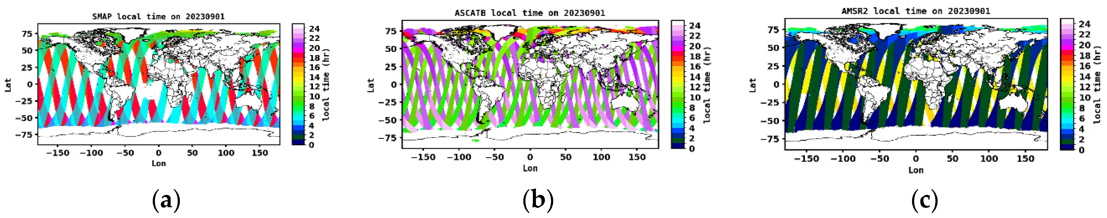
Figure 2.
Demonstration of local time (LT) coverages for CYGNSS at the indicated UT time, plus or minus 0.75 hours, on September 1, 2023.
Figure 2.
Demonstration of local time (LT) coverages for CYGNSS at the indicated UT time, plus or minus 0.75 hours, on September 1, 2023.
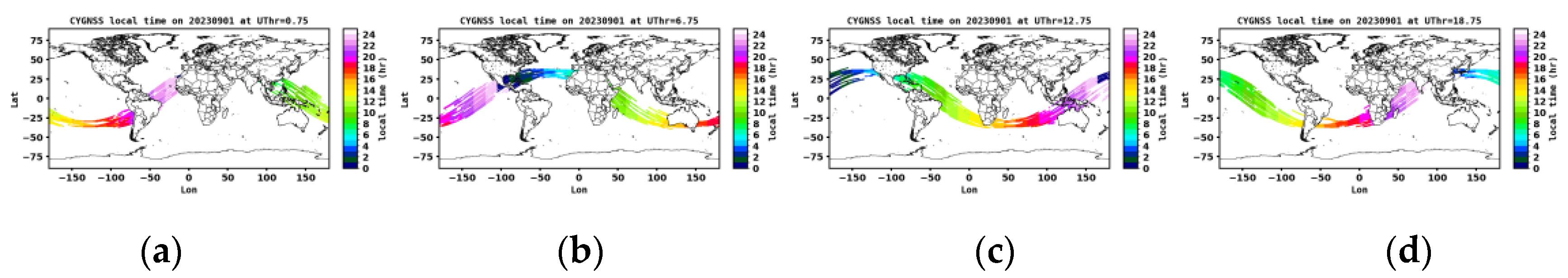
Figure 3.
Global hourly (4 UT hours per day from February to October 2023) pixel-by-pixel (0.25° × 0.25°) ocean wind speed maps are compared between CCMP and AMSR2, SMAP, ASCAT2, and CYGNSS, represented by different colors. (a)-(c) Histograms of the mean, standard deviation (STD), and standard error of the mean (SEM) of the percent differences. (d) Histograms of spatial correlation coefficients of these hourly maps. Note that in the legend, the median and standard deviation describe the current histogram's median and spread.
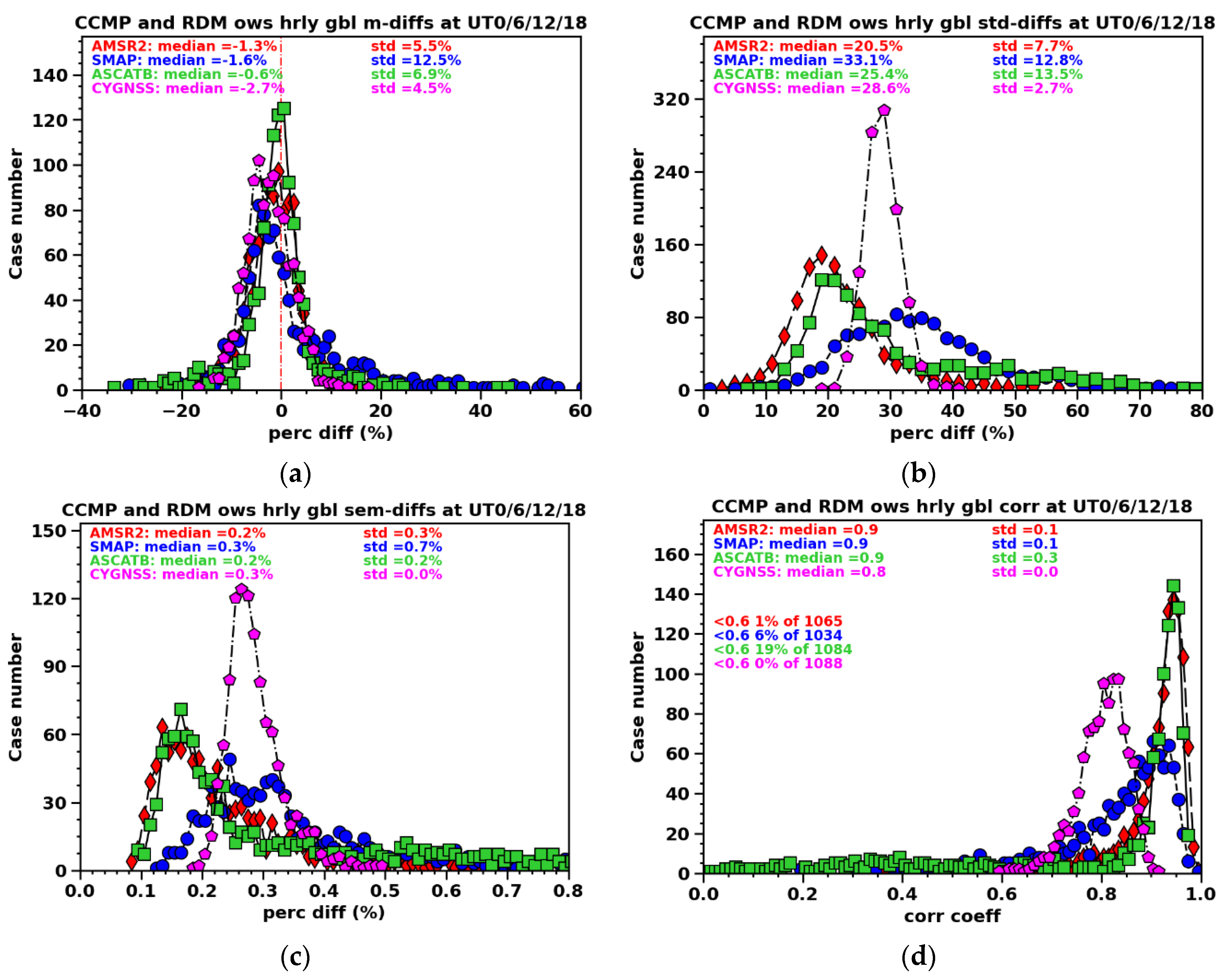
Figure 4.
CCMP is linearly interpolated from the 4 UTs onto 0.5-hourly intervals, and similar statistical moments of percent differences between CCMP and SMAP are calculated to compare with the results based on the 4 UTs per day. The maxima of the red histograms are adjusted (8-10 times) to match the blue curves. The y-axis numbers correspond to the blue histogram.
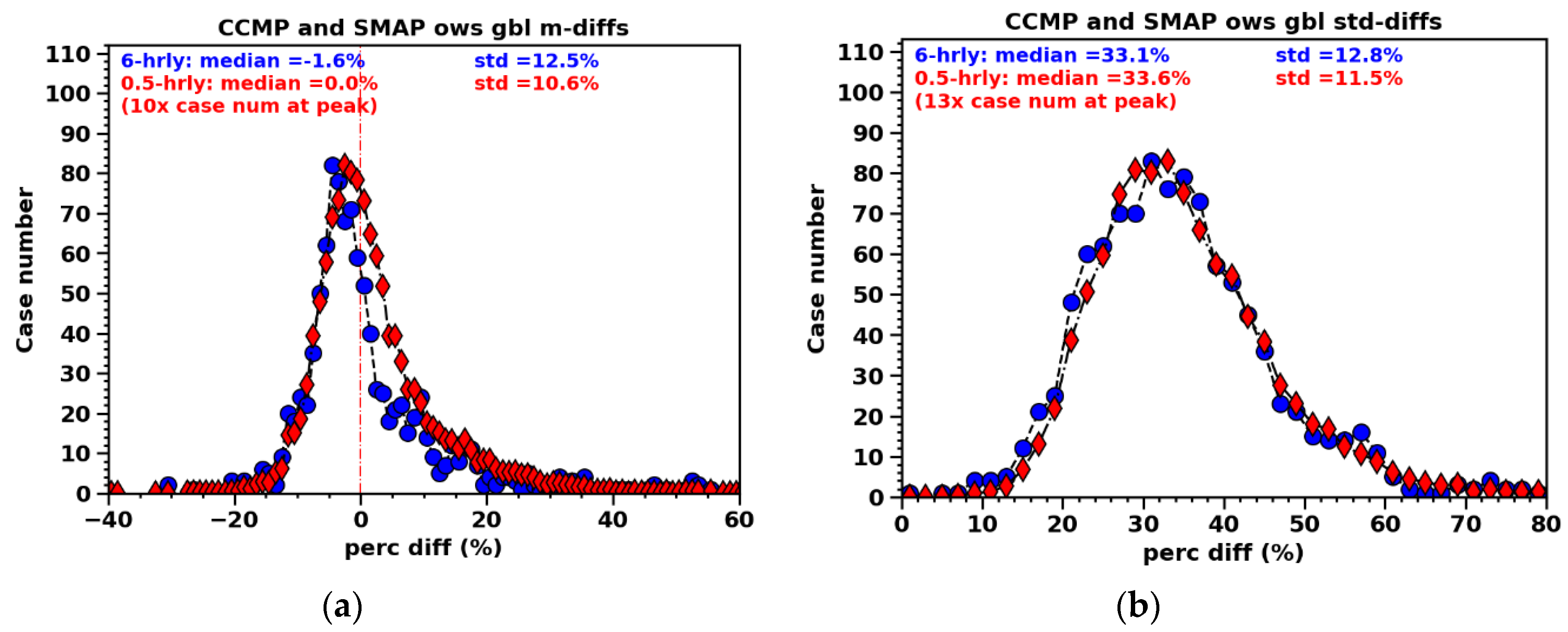
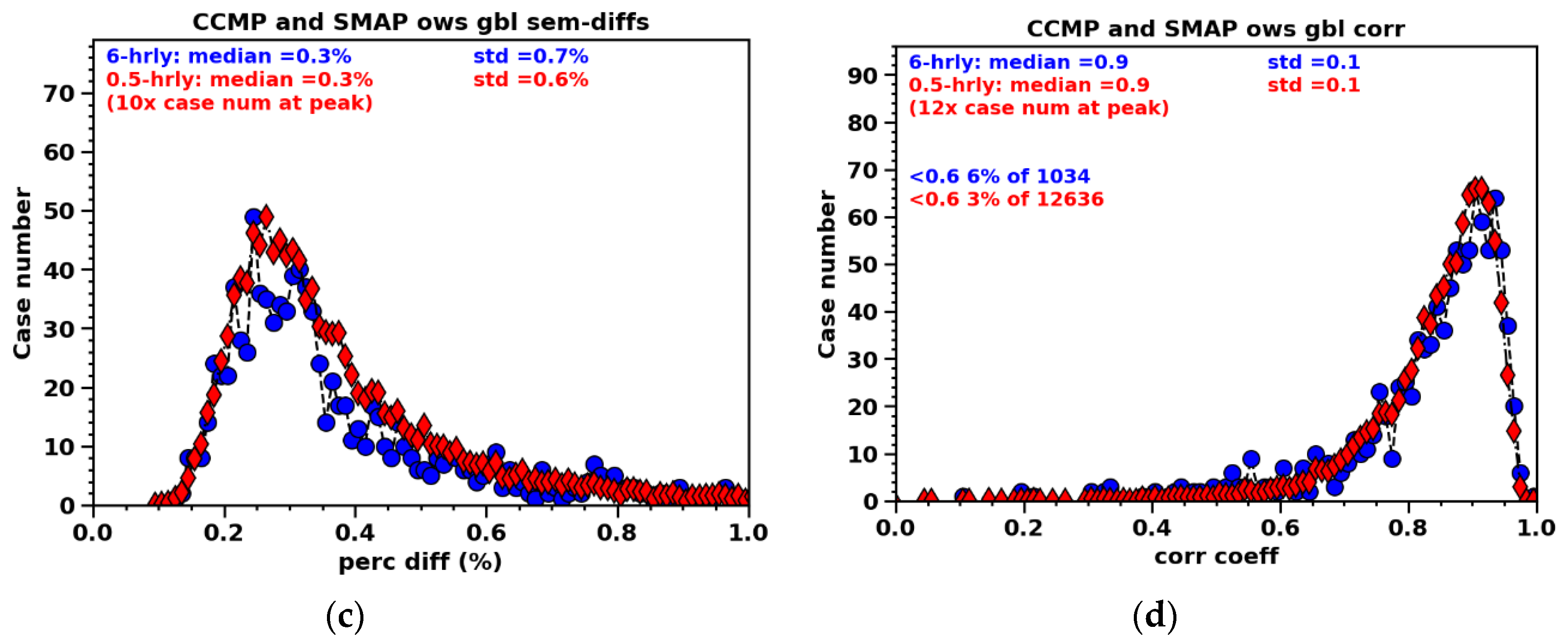
Figure 5.
The global map of CCMP for a selected day to demonstrate the distribution of high-wind structures. Both Saola and Haikui (within the white rectangle) are notable.
Figure 5.
The global map of CCMP for a selected day to demonstrate the distribution of high-wind structures. Both Saola and Haikui (within the white rectangle) are notable.
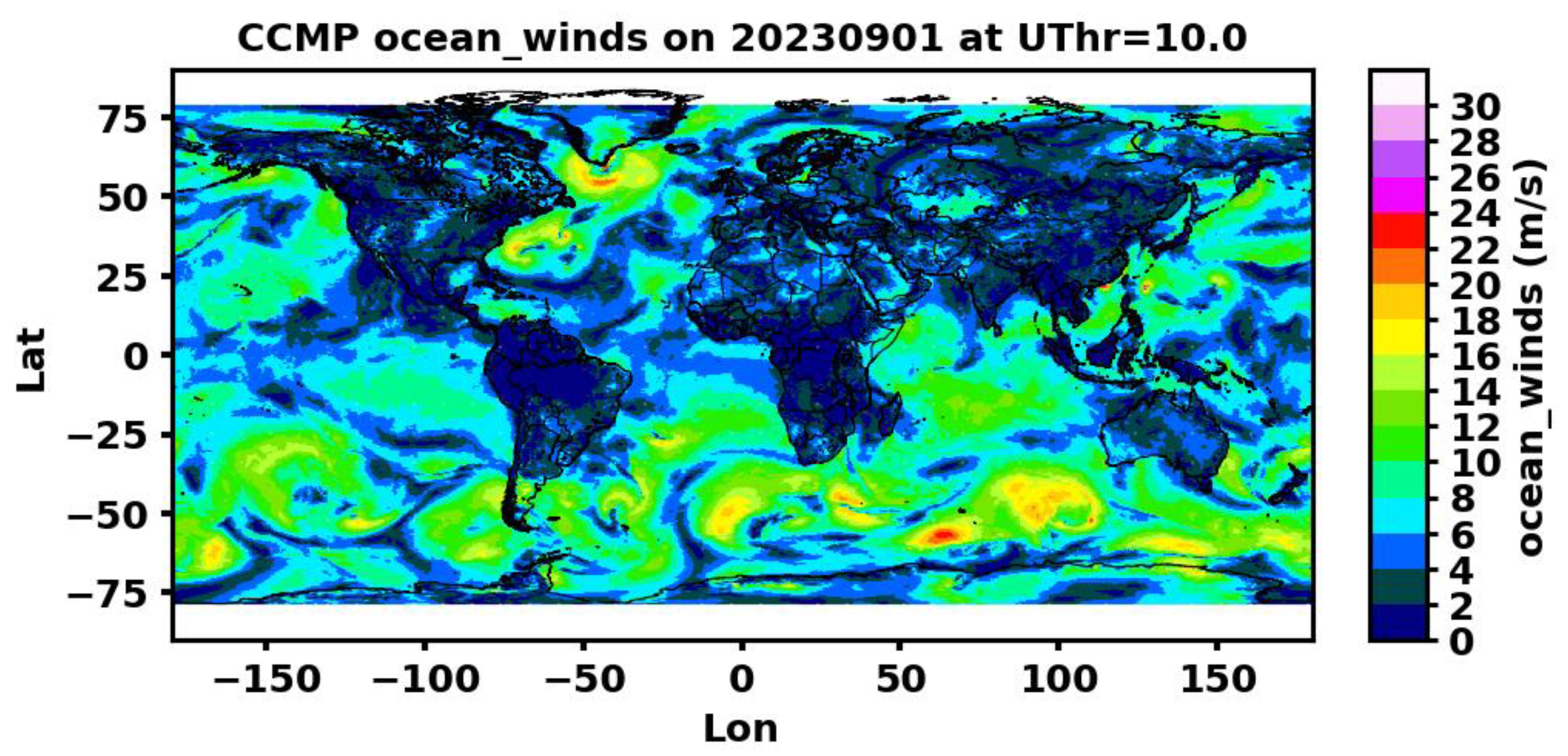
Figure 6.
Same as Figure 3, except that the individual cases are 10° Lon × 10° Lat blocks identified as containing high-wind structures (i.e., TCs) in the low-latitude region between 35° S and 35° N. CYGNSS is not included because, based on our criteria, no high-wind features were identified.
Figure 6.
Same as Figure 3, except that the individual cases are 10° Lon × 10° Lat blocks identified as containing high-wind structures (i.e., TCs) in the low-latitude region between 35° S and 35° N. CYGNSS is not included because, based on our criteria, no high-wind features were identified.
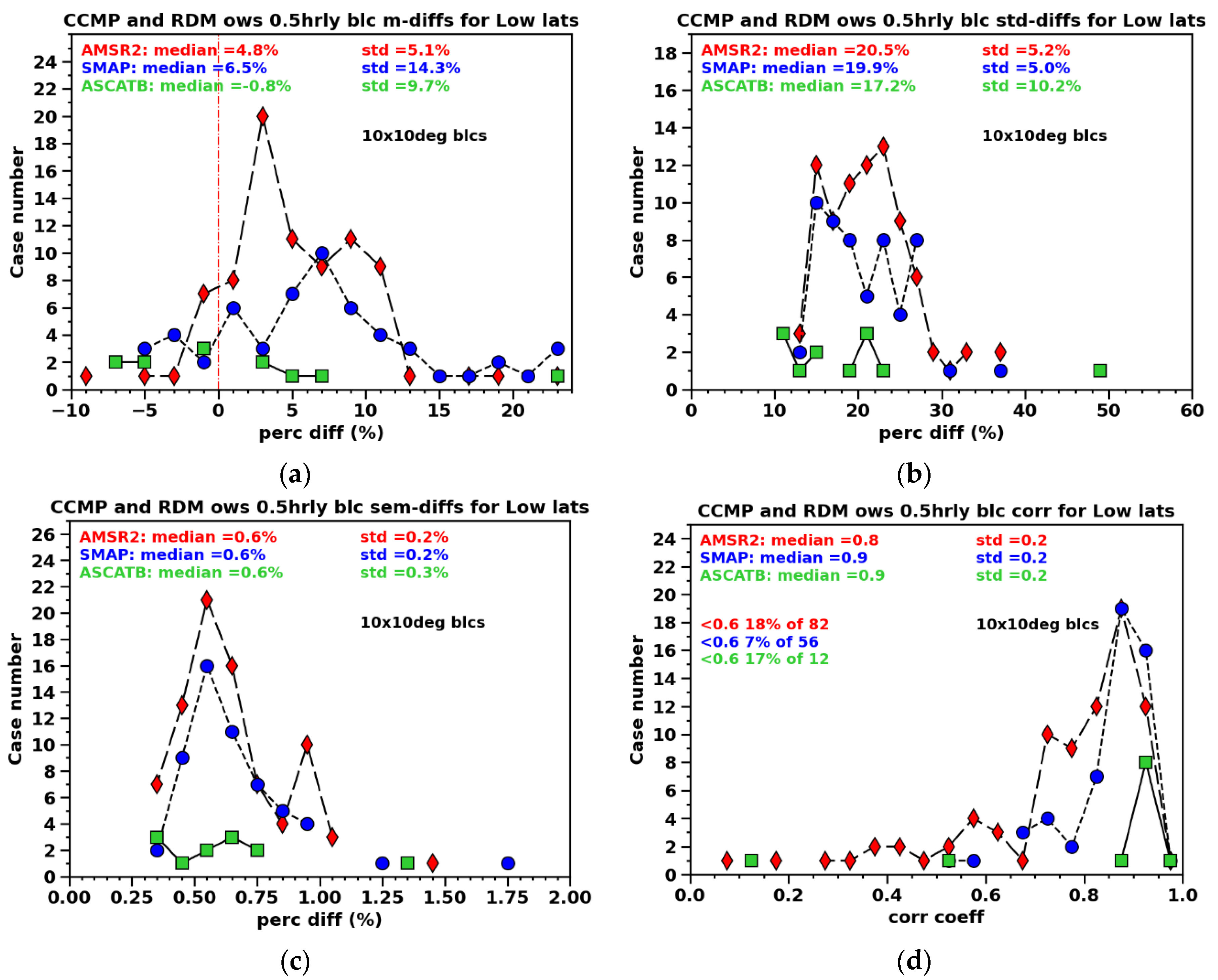
Figure 7.
AMSR2 maps (top) and CCMP maps (bottom) at coincidences for the five selected high spatial correlation cases, based on the results in Figure 6.
Figure 7.
AMSR2 maps (top) and CCMP maps (bottom) at coincidences for the five selected high spatial correlation cases, based on the results in Figure 6.
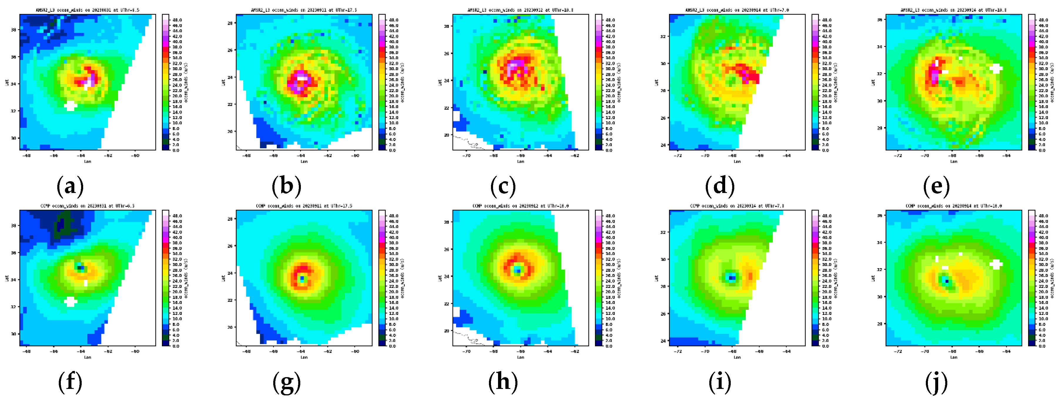
Figure 8.
Same as Figure 7, except for SMAP.
Figure 8.
Same as Figure 7, except for SMAP.
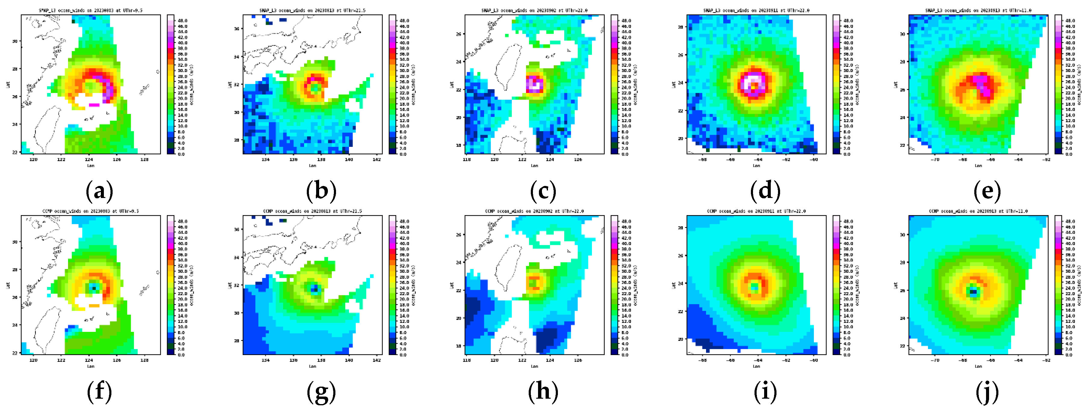
Figure 9.
Same as Figure 7, except for ASCATB.
Figure 9.
Same as Figure 7, except for ASCATB.
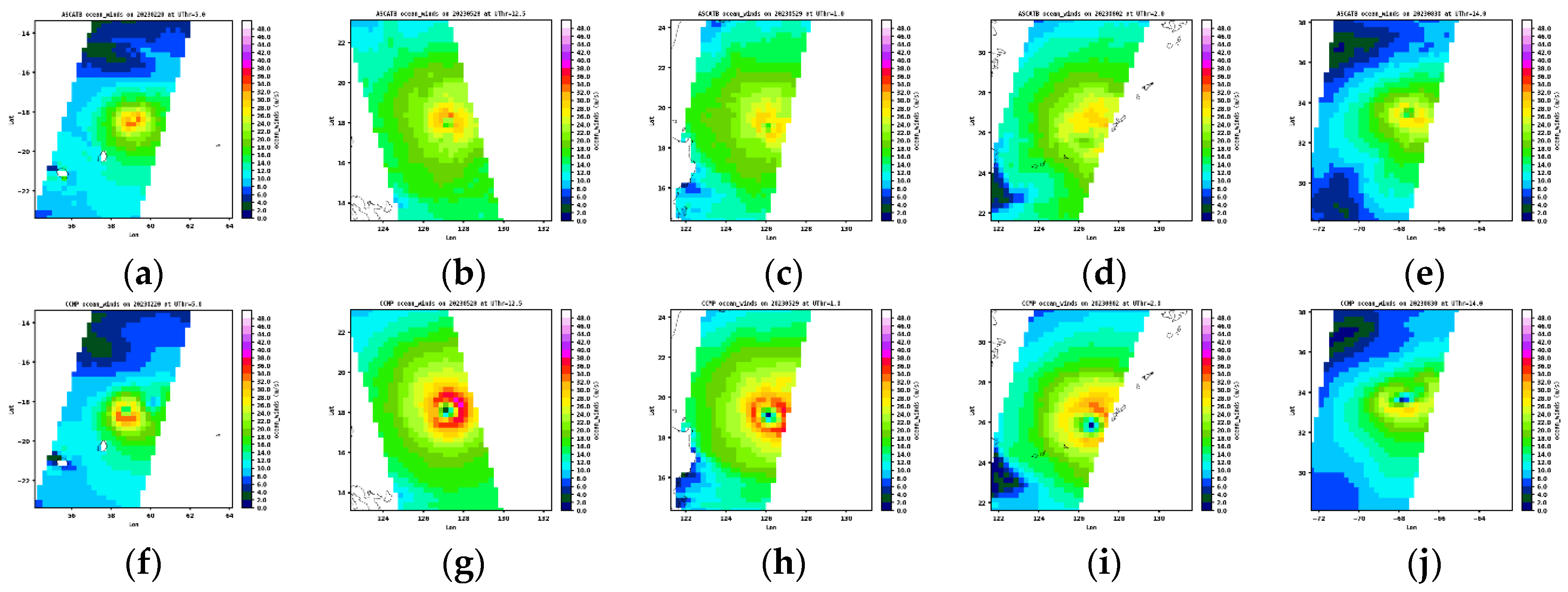
Figure 11.
AMSR2 maps (top) and CCMP maps (bottom) at coincidences for the five selected high spatial correlation cases in the mid-high latitude region, based on the results in Figure 10.
Figure 11.
AMSR2 maps (top) and CCMP maps (bottom) at coincidences for the five selected high spatial correlation cases in the mid-high latitude region, based on the results in Figure 10.
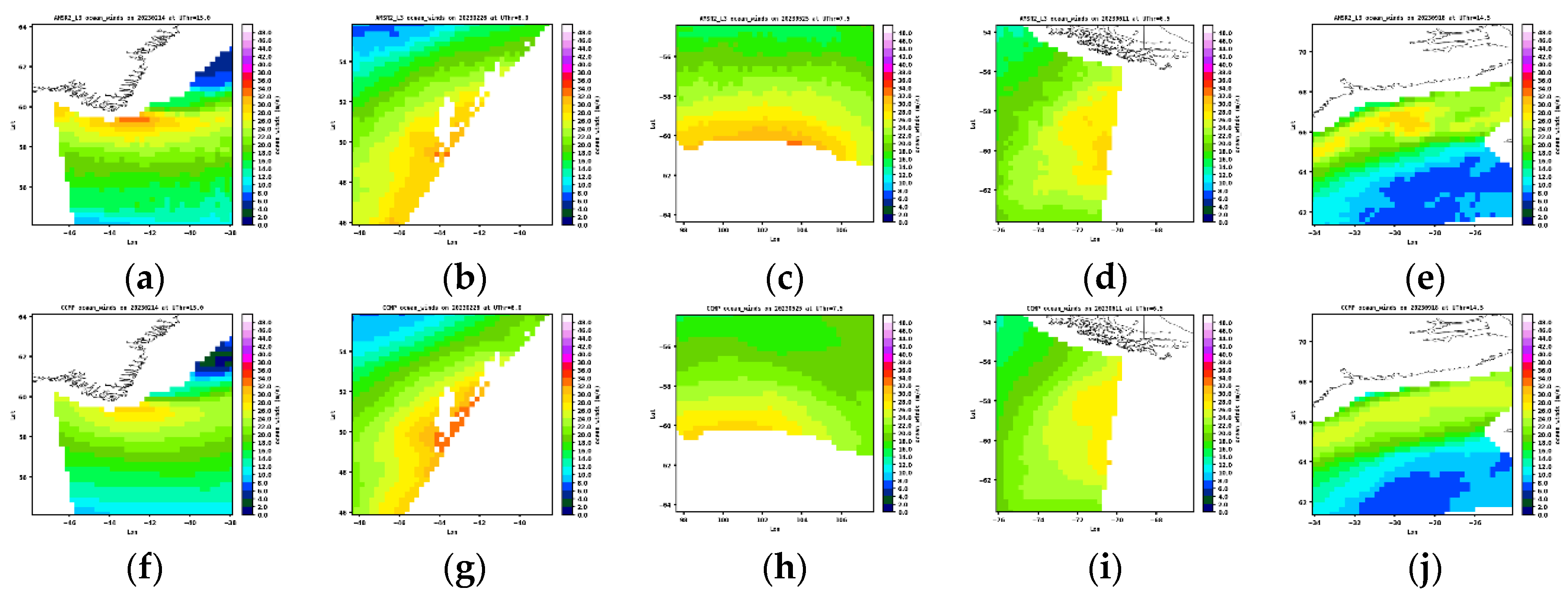
Figure 12.
Same as Figure 11, except for SMAP.
Figure 12.
Same as Figure 11, except for SMAP.
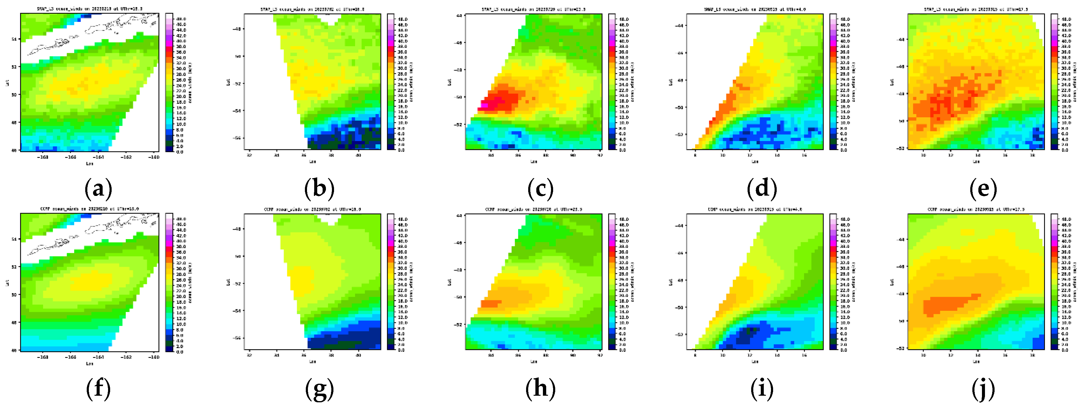
Figure 13.
Same as Figure 11 except for ASCATB.
Figure 13.
Same as Figure 11 except for ASCATB.
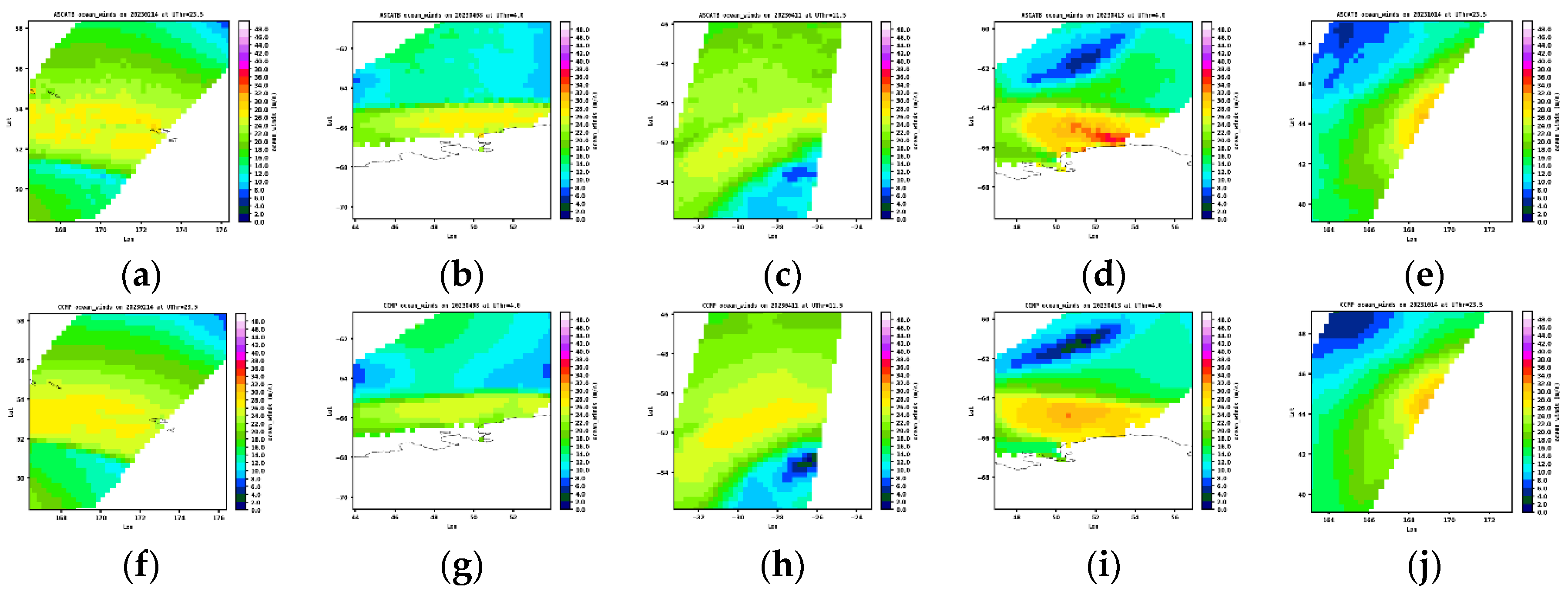
Figure 14.
Histograms of the statistics for the SAR and CCMP pixel-by-pixel ocean wind speed comparisons for individual tiles. (a-b) The histograms of tile-wise means, stds, and sems of the pixel-by-pixel percent differences. (c) Spatial correlations of CCMP and SAR ocean wind speed over individual SAR tiles. CCMP values are sampled over the SAR tiles, and the SAR data are resampled onto the 0.25° × 0.25° grid.
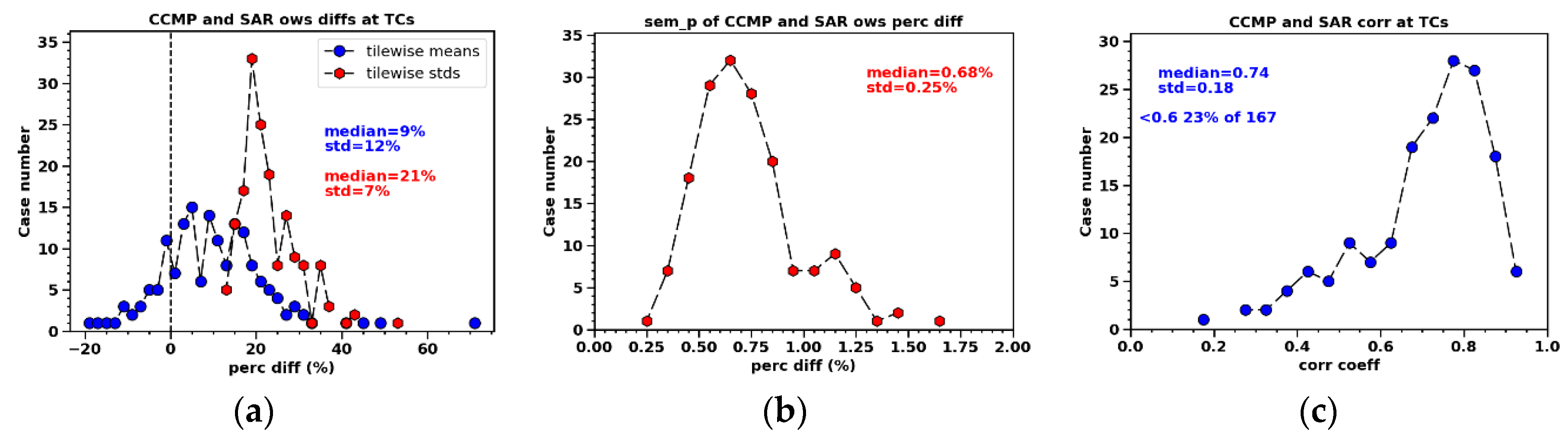
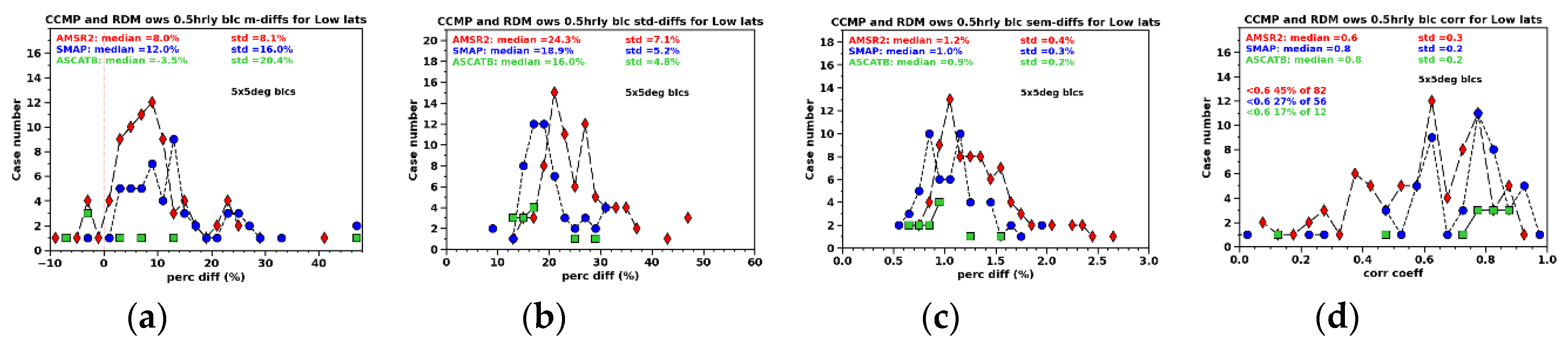
Figure 16.
Selected SAR and CCMP TC maps at coincidences with spatial correlations greater than 0.9.
Figure 16.
Selected SAR and CCMP TC maps at coincidences with spatial correlations greater than 0.9.
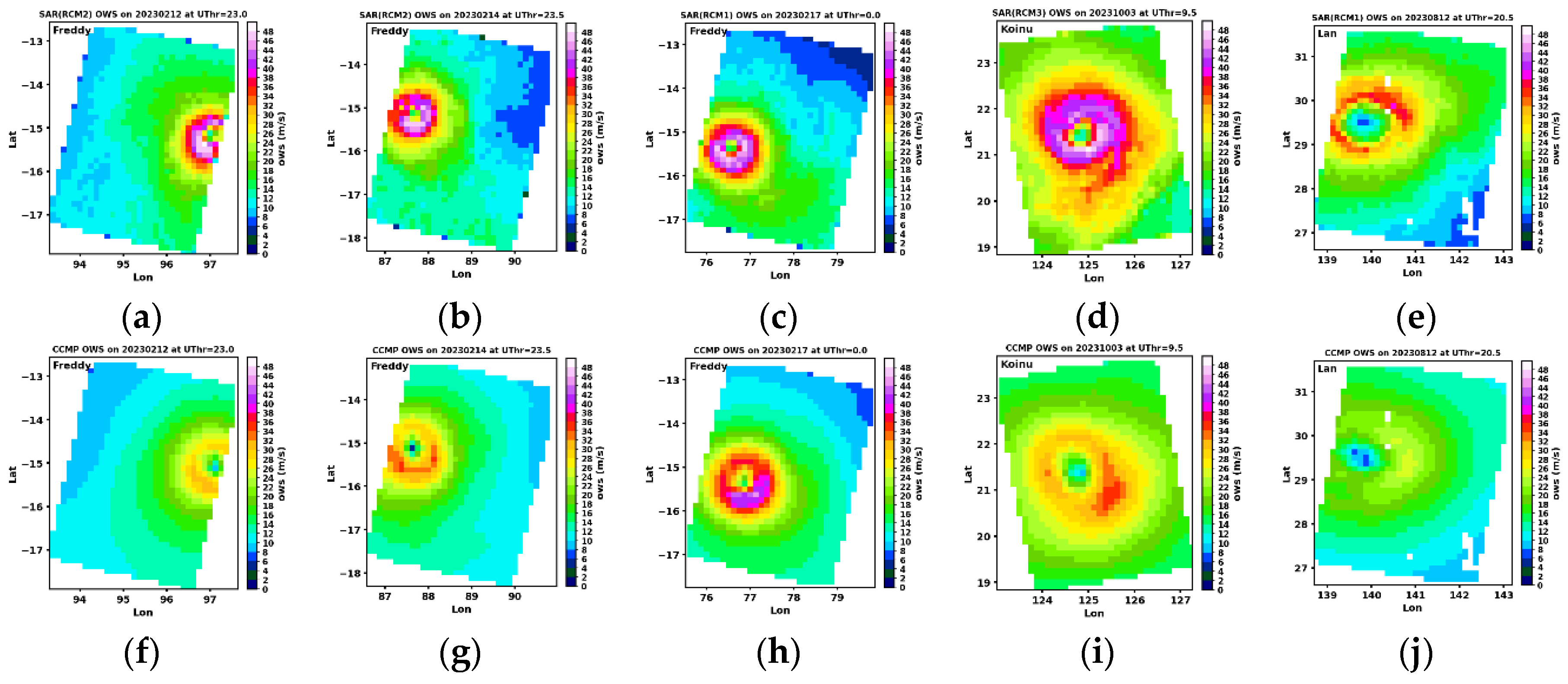
Figure 17.
Demonstration of the TC eye center and eye region identification routines. The yellow crosses are filled into the detected eye-region size, and the red circle marks the eye center position, which is generally the pixel that possesses the lowest ocean wind speed.
Figure 17.
Demonstration of the TC eye center and eye region identification routines. The yellow crosses are filled into the detected eye-region size, and the red circle marks the eye center position, which is generally the pixel that possesses the lowest ocean wind speed.
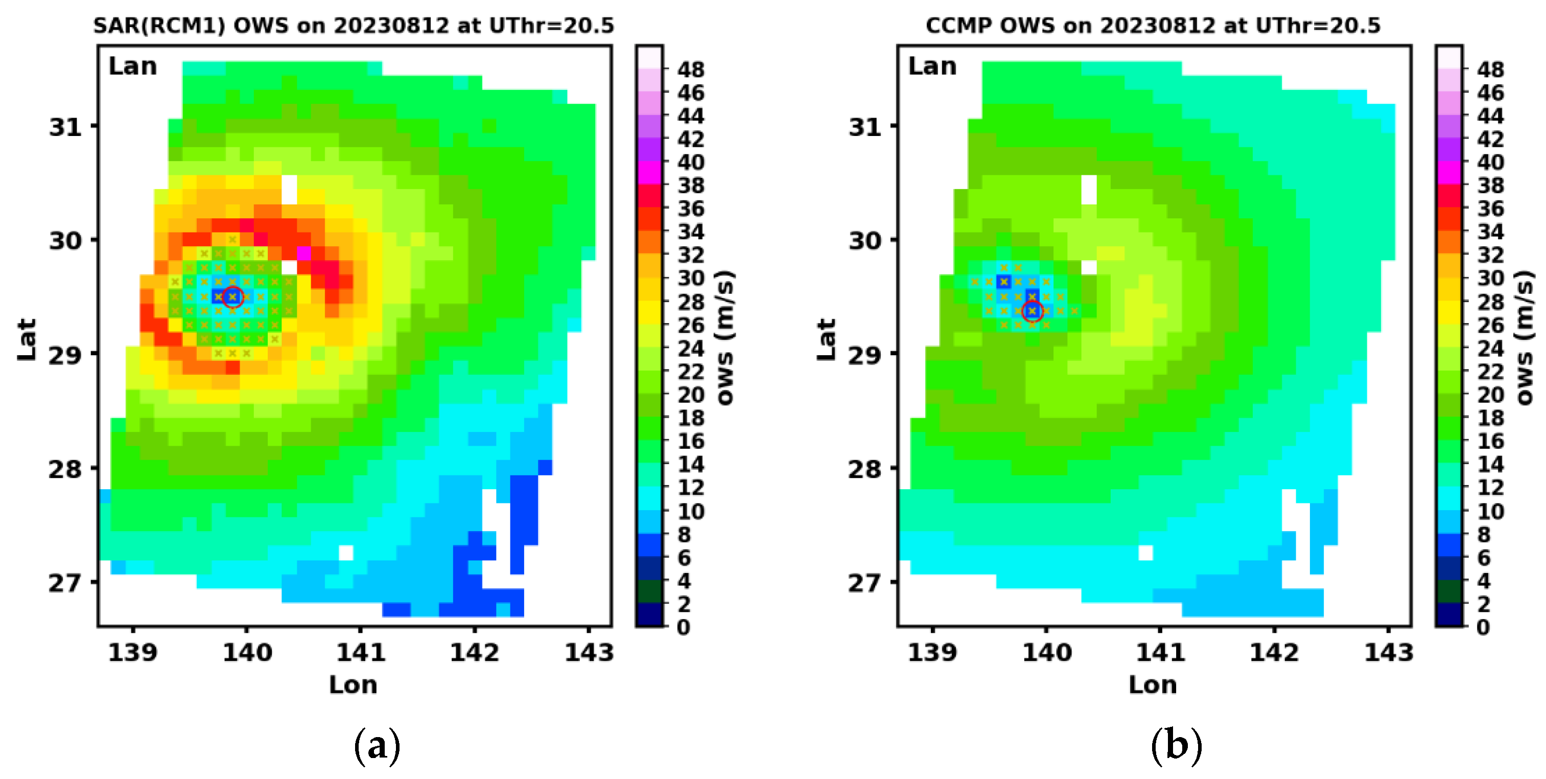
Figure 18.
SAR and CCMP TC equivalent radii for different ocean wind speed levels (2.0 m/s intervals) for the five pairs of maps shown in Figure 16.
Figure 18.
SAR and CCMP TC equivalent radii for different ocean wind speed levels (2.0 m/s intervals) for the five pairs of maps shown in Figure 16.
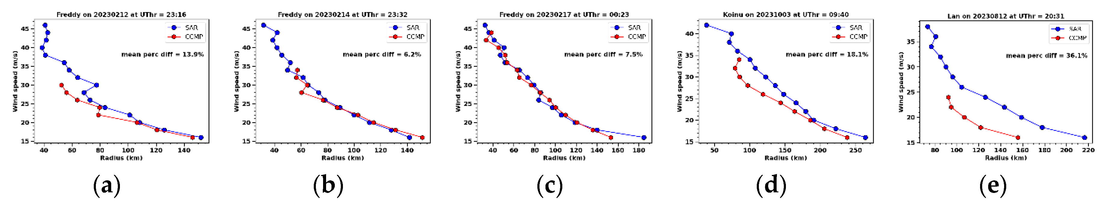
Figure 19.
TC structure comparisons between SAR and CCMP, via histograms of differences in TC eye-center locations (a), eye-region sizes (b), equivalent radii (c), and S-N and W-E asymmetries, using all coincident pairs throughout February-October 2023.
Figure 19.
TC structure comparisons between SAR and CCMP, via histograms of differences in TC eye-center locations (a), eye-region sizes (b), equivalent radii (c), and S-N and W-E asymmetries, using all coincident pairs throughout February-October 2023.
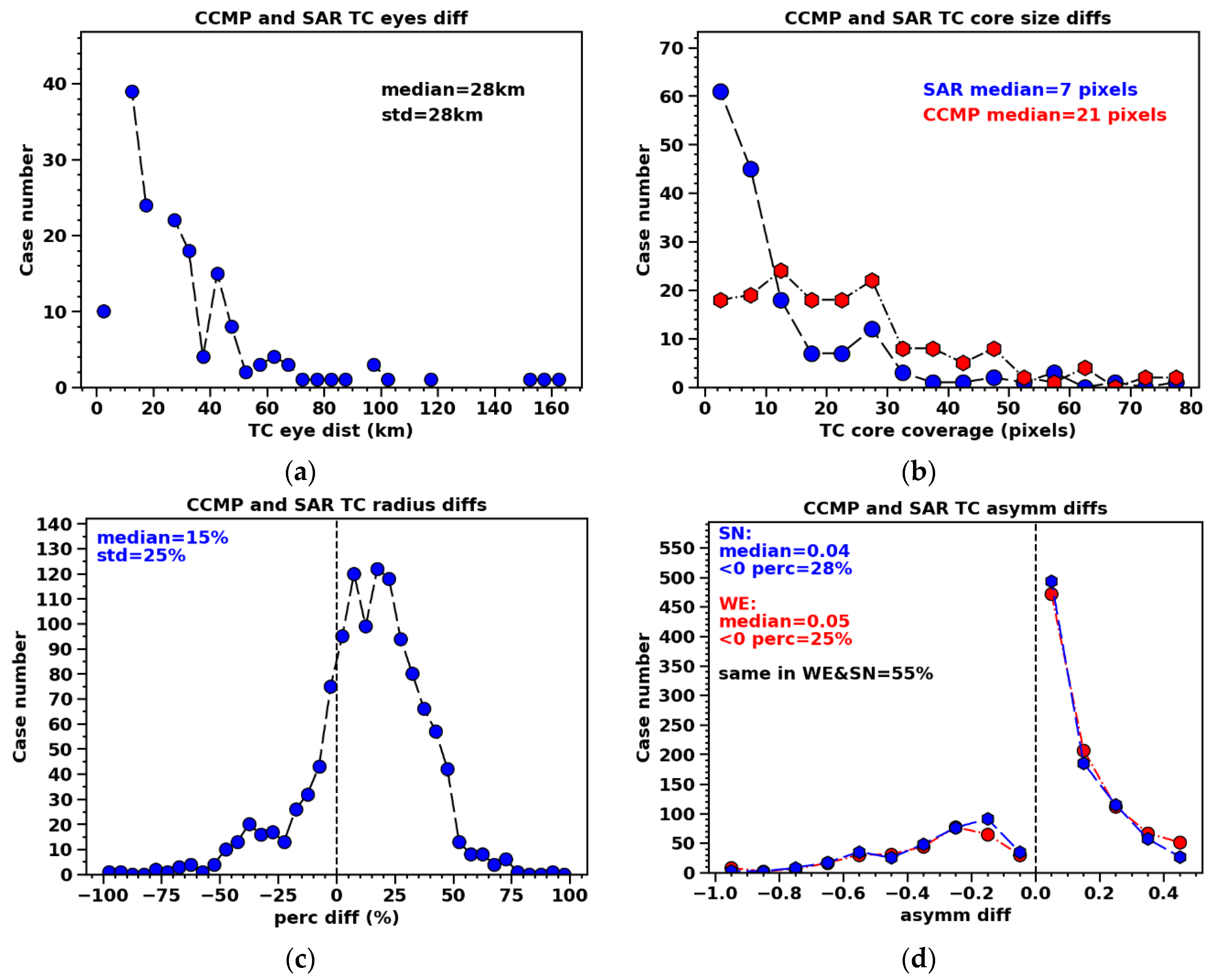
Figure 20.
(a) Agreement statistics of the training set (75% of ocean wind speed values for a set of TCs) using the random forest (RF) regressor approach to predict the ocean wind speed values (involved TCs) using the CCMP values at the coincidences. (b) the same statistics for the remaining 25% of values for the same set of TCs. (c) Agreement statistics when the RF model is applied to an independent set of TCs. The ty1&2 in the title refers to the case when all predictors in Table 2 are used for the RF model training.
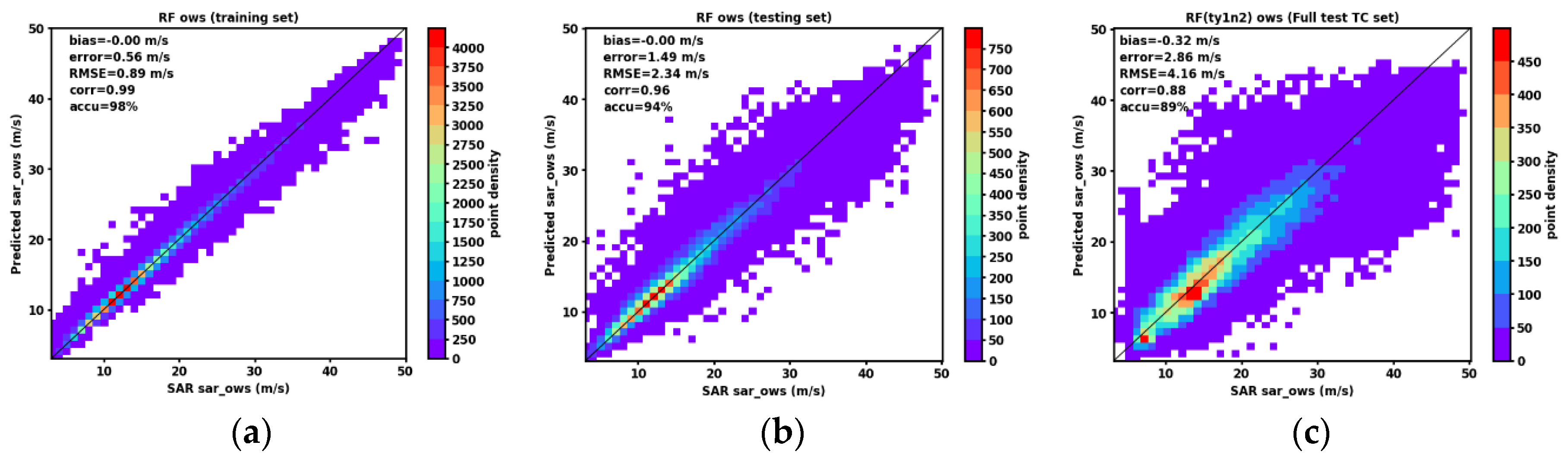
Figure 21.
Histograms of the statistics describing the improvement in the predicted ocean wind speed maps relative to the CCMP maps, assuming SAR maps are taken as the true states.
Figure 21.
Histograms of the statistics describing the improvement in the predicted ocean wind speed maps relative to the CCMP maps, assuming SAR maps are taken as the true states.
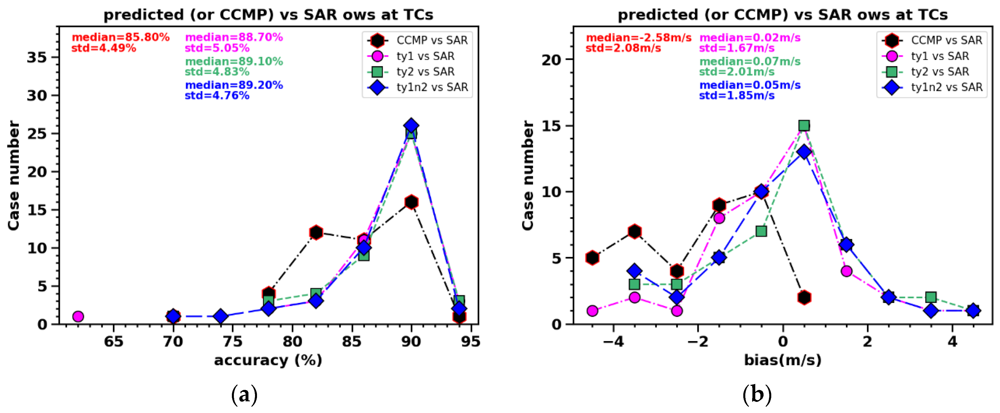
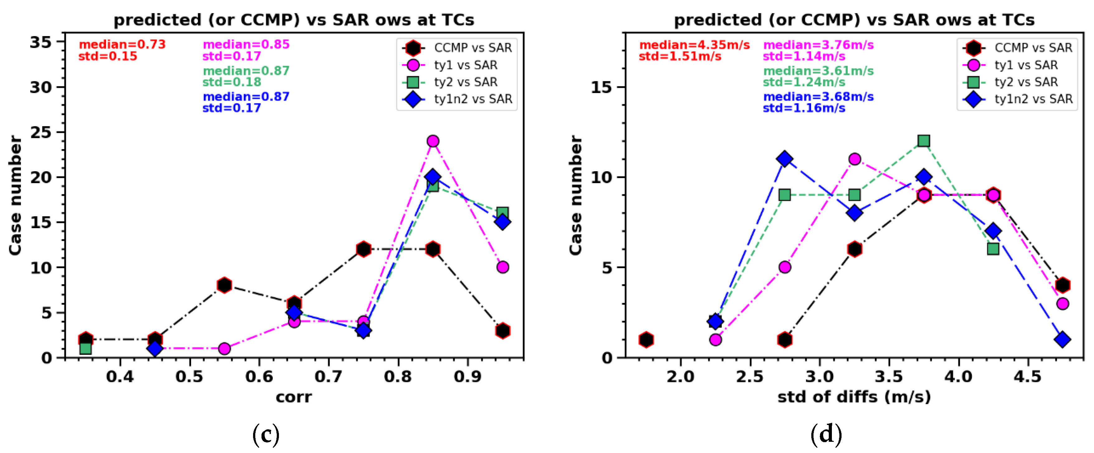
Figure 22.
Use three selected ocean wind speed tiles to demonstrate the performance of the ty1, ty2, and ty1&2 (3rd–5th columns) relative to SAR maps (1st column) and the CCMP maps (2nd column).
Figure 22.
Use three selected ocean wind speed tiles to demonstrate the performance of the ty1, ty2, and ty1&2 (3rd–5th columns) relative to SAR maps (1st column) and the CCMP maps (2nd column).
Disclaimer/Publisher’s Note: The statements, opinions and data contained in all publications are solely those of the individual author(s) and contributor(s) and not of MDPI and/or the editor(s). MDPI and/or the editor(s) disclaim responsibility for any injury to people or property resulting from any ideas, methods, instructions or products referred to in the content. |
© 2024 by the authors. Licensee MDPI, Basel, Switzerland. This article is an open access article distributed under the terms and conditions of the Creative Commons Attribution (CC BY) license (http://creativecommons.org/licenses/by/4.0/).
Copyright: This open access article is published under a Creative Commons CC BY 4.0 license, which permit the free download, distribution, and reuse, provided that the author and preprint are cited in any reuse.


