Finding a Research Paper Which Meaningfully Averages Unbounded Sets

1. Intro

Let $n\in \mathbb{N}$. Suppose $A\subseteq {\mathbb{R}}^n$ is Borel and $\mathcal{U}$ is the set of all unbounded A. Also, ${\dim }_{\mathrm{H}}(·)$ is the Hausdorff dimension and ${\mathcal{H}}^{{\dim }_{\mathrm{H}}(·)}(·)$ is the Hausdorff measure in its dimension on the Borel $\sigma$-algebra.

1.1. Special case of A

Suppose the n-dimensional box is B. How do we define explicit A, such that:

• ${\mathcal{H}}^n(A\cap B)>0$ for all B
• ${\mathcal{H}}^n(A\cap B)\ne {\mathcal{H}}^n\left(B\right)$ for all B?

This case of A is called $A^{\prime }$.

1.2. Attempting to Analyze/Average A

The expected value of A, w.r.t the Hausdorff measure in its dimension, is:

$$\mathrm{Avg}\left(A\right)={\displaystyle \frac{1}{{\mathcal{H}}^{{\dim }_{\mathrm{H}}\left(A\right)}\left(A\right)}}{\int }_A(x_1,···,x_n)d{\mathcal{H}}^{{\dim }_{\mathrm{H}}\left(A\right)}$$

(1)

Nevertheless, we have the following problems:

Note 1. (Problem 1) When $A=A^{\prime }$(§1.1), $\mathrm{Avg}\left(A^{\prime }\right)$ is undefined.

Note 2. (Problem 2) When ${\mathcal{U}}^{\prime }\subseteq \mathcal{U}$ is the set of all A with a finite $\mathrm{Avg}\left(A\right)$, where the cardinality is $|·|$, $|{\mathcal{U}}^{\prime }|<|\mathcal{U}|$ (i.e., ${\mathcal{U}}^{\prime }$ is “measure zero" in$\mathcal{U}$)

We fix both problems using this approach, where we discuss the term “satisfying" later:

1.2.1. Approach

We want an unique, satisfying extension of the expected value of A, w.r.t the Hausdorff measure in its dimension, on bounded sets to A, which takes finite values only, such that when ${\mathcal{U}}^{″}\subseteq \mathcal{U}$ is the set of all A with this extension:

• $|\mathcal{U}\setminus {\mathcal{U}}^{″}|<|{\mathcal{U}}^{″}|$ (i.e., ${\mathcal{U}}^{″}$ is “almost everywhere" in $\mathcal{U}$)
• If (1) isn’t true, then $|{\mathcal{U}}^{″}|=|\mathcal{U}\setminus {\mathcal{U}}^{″}|$

1.3. Question

Is there a unique way to define “satisfying" & “extension" in the approach, which solves Problems 1 and 2 with applications?

For an example, keep reading.

2. Extending the Expected Value of A w.r.t the Hausdorff Measure

The following are two methods to finding the most generalized, satisfying extension of $\mathrm{Avg}\left(A\right)$ in eq. 1 which we later use to answer §1.3:

• One way is defining a generalized, satisfying extension of the Hausdorff measure, on all A with positive & finite measure which takes positive, finite values for all Borel A. This can theoretically be done in the paper “A Multi-Fractal Formalism for New General Fractal Measures"[1], where in Equation (1) we replace the Hausdorff measure with the extended Hausdorff measure.
• Another way is finding generalized, satisfying average of all A in the fractal setting. This can be done with the papers “Analogues of the Lebesgue Density Theorem for Fractal Sets of Reals and Integers" [2] and “Ratio Geometry, Rigidity and the Scenery Process for Hyperbolic Cantor Sets" [3] where we take the expected value of A w.r.t the densities in [2,3].

Note, neither approach answers §1.3 since they can’t solve Problems 1 and 2 (i.e., $\mathcal{U}$ is the set of all unbounded A). Therefore, we ask a leading question using §2 to guide the reader to an interesting solution to §1.3.

3. Attempt to Define “Unique and Satisfying" in The Approach of §1.2

3.1. Note

Before reading, when §3.2 is unclear, see §5 for clarity. In §5, we define:

• “Set theoretic limit" (§5.1)
• “Expected value on sequences of bounded sets" (§5.2)
• “Equivelant sequences of bounded sets" (§5.3, Definition 1)
• “Nonequivelant sequences of bounded sets" (§5.3, Definition 2)
• The “measure" on a sequence of bounded sets which increases at a rate linear or superlinear to that of “non-equivelant" sequences of bounded sets (§5.4.1, §5.4.2)
• The “actual" rate of expansion on a sequence of bounded sets (§5.5)

3.2. Leading Question

To define unique and satisfying inside the approach of §1.2, we take the expected value of a sequence of bounded sets chosen by a choice function. To find the choice function, we ask the leading question...

If we make sure to:

(A)

See §3.1 and (C)-(E) when something is unclear

(B)

Take all sequences of bounded sets whose “set theoretic limit" is A

(C)

Define C to be chosen center point of ${\mathbb{R}}^n$

(D)

Define E to be the chosen, fixed rate of expansion of a sequence of bounded sets

(E)

Define $\mathcal{E}$ to be actual rate of expansion of a sequence of bounded sets (§5.5)

Does there exist a unique choice function which chooses the set of all equivalent sequences of bounded sets where:

• The chosen, equivelant sequences of bounded sets should satisfy (B).
• The “measure" of all the chosen, equivalent sequences of bounded sets which satisfy (1) should increase at a rate linear or superlinear to that of non-equivalent sequences of bounded sets satisfying (B).
• The expected values, defined in the papers of §2, for all equivalent sequences of bounded sets are equivalent and finite
• For the chosen, equivalent sequences of bounded sets satisfying (1)–(3).
  • The n-d Euclidean distance between criteria (3) and C is the less than or equal to that of all the non-equivalent sequences of bounded sets satisfying (1)–(3)
  • The “rate of divergence" [4, p.275-322] of $\left|\left|\mathcal{E}-E\right|\right|$, using the absolute value $\left|\right|·\left|\right|$, is less than or equal to that of all the non-equivalent sequences of bounded sets which satisfy (1)–(3)
• When set ${\mathcal{U}}^{″}\subseteq \mathcal{U}$ is the set of all A, where the choice function chooses the set of all equivalent sequences of bounded sets satisfying (1)–(4), then:
  • $|\mathcal{U}\setminus {\mathcal{U}}^{″}|<|\mathcal{U}|$
  • When $|\mathcal{U}\setminus {\mathcal{U}}^{″}|\neg <|\mathcal{U}|$, then $|{\mathcal{U}}^{″}|=|\mathcal{U}\setminus {\mathcal{U}}^{″}|$
• Out of all choice functions which satisfy (1)–(5) we choose the one with the simplest form, meaning for each choice function fully expanded, we take the one with the fewest variables/numbers?

(In case this is unclear, see §5.)

I’m convinced the expected values of the sequences of bounded sets chosen by a choice function which answers the leading question aren’t unique nor satisfying enough to answer Problems 1 and 2. Still, adjustments are possible by changing the criteria or by adding new criteria to the question.

4. Question Regarding My Work

Most don’t have time to address everything in my research, hence I ask the following:

Is there a research paper which already solves the ideas I’m working on? (Non-published papers, such as mine [5], don’t count.)

Using AI, papers that might answer this question are “Prediction of dynamical systems from time-delayed measurements with self-intersections" [6] and “A Hausdorff measure boundary element method for acoustic scattering by fractal screens" [7].

Does either of these papers solve Problems 1 and 2 with applications?

5. Clarifying §3

Let $A\subseteq {\mathbb{R}}^n$ be an unbounded, Borel set. Suppose ${\dim }_{\mathrm{H}}(·)$ be the Hausdorff dimension and ${\mathcal{H}}^{{\dim }_{\mathrm{H}}(·)}(·)$ be the Hausdorff measure in its dimension on the Borel $\sigma$-algebra. See §3.2, once reading this section, and consider the following:

Is there a simpler version of the definitions below?

5.1. Set Theoretic Limit of a Sequence of Bounded Sets

Note the set theoretic limit of a sequence of sets of bounded set ${\left(F_r\right)}_{r\in \mathbb{N}}$ is A when:

$$\begin{array}{c}\underset{r\to \infty }{lim\; sup}{F}_r=\bigcap _{r\ge 1}\bigcup _{q\ge r}{F}_q\\ \underset{r\to \infty }{lim\; inf}{F}_r=\bigcup _{r\ge 1}\bigcap _{q\ge r}{F}_q\end{array}$$

where:

$$\underset{r\to \infty }{lim\; sup}{F}_r=\underset{r\to \infty }{lim\; inf}{F}_r=A$$

5.2. Expected Value of Bounded Sequences of Sets

If ${\left(F_r\right)}_{r\in \mathbb{N}}$ is a sequence of bounded sets whose set-theoretic limit is A (§5.1), the expected value of A w.r.t ${\left(F_r\right)}_{r\in \mathbb{N}}$ is $\mathrm{Avg}\left(F_r\right)$ (when it exists) where:

$$\begin{array}{cc}\hfill & \forall (ϵ>0)\exists (N\in \mathbb{N})\forall (r\in \mathbb{N})\left(r\ge N\Rightarrow \left|{\displaystyle \frac{1}{{\mathcal{H}}^{{\dim }_{\mathrm{H}}\left(F_r\right)}\left(F_r\right)}}{\int }_{F_r}(x_1,···,x_n)d{\mathcal{H}}^{{\dim }_{\mathrm{H}}\left(F_r\right)}-\mathrm{Avg}\left(F_r\right)\right|<ϵ\right)\hfill \end{array}$$

(2)

Note, $\mathrm{Avg}\left(F_r\right)$ can be extended by using §2.

5.3. Defining Equivelant and Non-Equivelant Sequences of Bounded Functions

The sequences below are sequences of sets with a set theoretic limit (§5.1) of A:

$$\overrightarrow{F_1}={\left(F_{r_1}^{\left(1\right)}\right)}_{r_1\in \mathbb{N}},\overrightarrow{F_2}={\left(F_{r_2}^{\left(2\right)}\right)}_{r_2\in \mathbb{N}},···,\overrightarrow{F_s}={\left(F_{r_s}^{\left(s\right)}\right)}_{r_s\in \mathbb{N}}$$

Thus, we define:

Definition 1.

[Equivelant Sequences of Bounded Sets] Suppose, $S\subseteq \mathbb{N}$ is an arbitrary set. Note, the sequences of bounded sets in:

$$\left\{\overrightarrow{F_s}:s\in S\right\}$$

are equivalent, if for all $k,v\in S$, where $k\ne v$, $\overrightarrow{F_k}$ and $\overrightarrow{F_v}$ are equivelant: i.e., there exists a $N^{\prime }\in \mathbb{N}$, such for all $r_k\ge N^{\prime }$, there is a $r_v\in \mathbb{N}$, where:

$${\mathcal{H}}^{{\dim }_{\mathrm{H}}\left(F_{r_k}^{\left(k\right)}\right)}(F_{r_k}^{\left(k\right)}\Delta F_{r_v}^{\left(v\right)})=0$$

and for all  $r_v\ge N^{\prime }$, there is a  $r_k\in \mathbb{N}$, where:

$${\mathcal{H}}^{{\dim }_{\mathrm{H}}\left(F_{r_v}^{\left(v\right)}\right)}(F_{r_k}^{\left(k\right)}\Delta F_{r_v}^{\left(v\right)})=0$$

More, for each  $s\in \mathbb{N}$, we denote all equivalent sequences of bounded functions to  ${\left(F_{r_s}^{\left(s\right)}\right)}_{r_s\in \mathbb{N}}$  using the notation

$$\sim {\left(F_{r_s}^{\left(s\right)}\right)}_{r_s\in \mathbb{N}}$$

If the sequence of sets in:

$$\left\{\overrightarrow{F_s}:s\in S\right\}$$

are equivalent, then for all $k,v\in S$, where $k\ne v$:

$$\mathrm{Avg}\left(F_{r_k}^{\left(k\right)}\right)=\mathrm{Avg}\left(F_{r_v}^{\left(v\right)}\right)\left(\S 5.2\right)$$

Note, this explains criteria (3) in §3.

Definition 2.

[Non-Equivalent Sequences of Bounded Sets] Again, suppose $S\subseteq \mathbb{N}$ is an arbitrary set. Then, the sequences of bounded sets in:

$$\left\{\overrightarrow{F_s}:s\in S\right\}$$

are non-equivalent, if Definition 1 is false, meaning for some $k,v\in S$, where $k\ne v$, $\overrightarrow{F_k}$ and $\overrightarrow{F_v}$ are non-equivelant: there is a $N^{\prime }\in \mathbb{N}$, where for all $r_k\ge N^{\prime }$, there is either a $r_v\in \mathbb{N}$, where:

$${\mathcal{H}}^{{\dim }_{\mathrm{H}}\left(F_{r_k}^{\left(k\right)}\right)}(F_{r_k}^{\left(k\right)}\Delta F_{r_v}^{\left(v\right)})\ne 0$$

or for all  $r_v\ge N^{\prime }$, there is a  $r_k\in \mathbb{N}$, where

$${\mathcal{H}}^{{\dim }_{\mathrm{H}}\left(F_{r_v}^{\left(v\right)}\right)}(F_{r_k}^{\left(k\right)}\Delta F_{r_v}^{\left(v\right)})\ne 0$$

5.4. Defining the “Measure"

5.4.1. Preliminaries

We define the “measure" of ${\left(F_r\right)}_{r\in \mathbb{N}}$ in §5.4.2. To understand this “measure", keep reading. (In case the steps are unclear, see §8 for examples.)

• For every $r\in \mathbb{N}$, “over-cover" $F_r$ with minimal, pairwise disjoint sets of equal ${\mathcal{H}}^{{\dim }_{\mathrm{H}}\left(F_r\right)}$ measure. (We denote the equal measures $\epsilon$, where the former sentence is defined $\mathbf{C}(\epsilon ,F_r,\omega )$: i.e., $\omega \in {\Omega }_{\epsilon ,r}$ enumerates all collections of these sets covering $F_r$. In case this step is unclear, see §8.1.)
• For every $\epsilon$, r and $\omega$, take a sample point from each set in $\mathbf{C}(\epsilon ,F_r,\omega )$. The set of these points is “the sample" which we define $\mathcal{S}(\mathbf{C}(\epsilon ,F_r,\omega ),\psi )$: i.e., $\psi \in {\Psi }_{\epsilon ,r,\omega }$ enumerates all possible samples of $\mathbf{C}(\epsilon ,F_r,\omega )$. (In the case this is unclear, see §8.2.)
• For every $\epsilon$, r, $\omega$ and $\psi$,

  (a)

  Take a “pathway” of line segments: we start with a line segment from arbitrary point $x_0$ of $\mathcal{S}(\mathbf{C}(\epsilon ,F_r,\omega ),\psi )$ to the sample point with smallest n-dimensional Euclidean distance to $x_0$ (i.e., when more than one sample point has smallest n-dimensional Euclidean distance to $x_0$, take either of those points). Next, repeat this process until the “pathway” intersects with every sample point once. (If this is unclear, see §8.3.1.)

  (b)

  Take the set of the length of all segments in (3a), except for lengths that are outliers [8]. Define this $\mathcal{L}(x_0,\mathcal{S}(\mathbf{C}(\epsilon ,F_r,\omega ),\psi ))$. (In the case this is unclear, see §8.3.2.)

  (c)

  Multiply remaining lengths in the pathway by a constant so they add up to one (i.e., a probability distribution). This will be denoted $\mathbb{P}\left(\mathcal{L}(x_0,\mathcal{S}(\mathbf{C}(\epsilon ,F_r,\omega ),\psi ))\right)$. (In case this step is unclear, see §8.3.3.)

  (d)

  Take the shannon entropy [9, p.61-95] of step (3c). We define this:

  $$\mathrm{E}\left(\mathbb{P}\left(\mathcal{L}(x_0,\mathcal{S}(\mathbf{C}(\epsilon ,F_r,\omega ),\psi ))\right)\right)=\sum _{x\in \mathbb{P}\left(\mathcal{L}(x_0,\mathcal{S}(\mathbf{C}(\epsilon ,F_r,\omega ),\psi ))\right)}-x{log}_{2}x$$

  which will be shortened to $\mathrm{E}\left(\mathcal{L}(x_0,\mathcal{S}(\mathbf{C}(\epsilon ,F_r,\omega ),\psi ))\right)$. (In case this is unclear, see §8.3.4)

  (e)

  Maximize the entropy w.r.t all "pathways". This we will denote:

  $$\mathrm{E}\left(\mathcal{L}\left(\mathcal{S}(\mathbf{C}(\epsilon ,F_r,\omega ),\psi )\right)\right)=\underset{x_0\in \mathcal{S}(\mathbf{C}(\epsilon ,F_r,\omega ),\psi )}{sup}\mathrm{E}\left(\mathcal{L}(x_0,\mathcal{S}(\mathbf{C}(\epsilon ,F_r,\omega ),\psi ))\right)$$

  (In case this step is unclear, see §8.3.5.)
• Therefore, the maximum entropy of ${\left(F_r\right)}_{r\in \mathbb{N}}$ w.r.t $\epsilon$, using (1) and (2) is:

  $${\mathrm{E}}_{\max }(\epsilon ,r)=\underset{\omega \in {\Omega }_{\epsilon ,r}}{sup}\underset{\psi \in {\Psi }_{\epsilon ,r,\omega }}{sup}\mathrm{E}\left(\mathcal{L}\left(\mathcal{S}(\mathbf{C}(\epsilon ,F_r,\omega ),\psi )\right)\right)$$

5.4.2. What Am I Measuring?

Suppose we define two sequences of bounded functions which have a set theoretic limit of A: e.g., ${\left(F_r^{★}\right)}_{r\in \mathbb{N}}$ and ${\left(F_j^{★★}\right)}_{j\in \mathbb{N}}$, where for constant $\epsilon$ and cardinality $|·|$

(a)

Using (2) and (33e) of section 5.4.1, suppose:

$$\begin{array}{cc}& \underline{\left|\mathcal{S}(\mathbf{C}(\epsilon ,F_r^{★},\omega ),\psi )\right|}=\hfill \\ \hfill & sup\left\{\left|\mathcal{S}(\mathbf{C}(\epsilon ,F_j^{★★},{\omega }^{\prime }),{\psi }^{\prime })\right|:j\in \mathbb{N},{\omega }^{\prime }\in {\Omega }_{\epsilon ,j},{\psi }^{\prime }\in {\Psi }_{\epsilon ,j,\omega },\mathrm{E}\left(\mathcal{L}\left(\mathcal{S}(\mathbf{C}(\epsilon ,F_j^{★★},{\omega }^{\prime }),{\psi }^{\prime })\right)\right)\le \mathrm{E}\left(\mathcal{L}\left(\mathcal{S}(\mathbf{C}(\epsilon ,F_r^{★},\omega ),\psi )\right)\right)\right\}\hfill \end{array}$$

then (using $\underline{\left|\mathcal{S}(\mathbf{C}(ϵ,F_r^{★},\omega ),\psi )\right|}$) we get

$$\overline{\alpha }\left(\epsilon ,r,\omega ,\psi \right)=\left|\mathcal{S}(\mathbf{C}(\epsilon ,F_r^{★},\omega ),\psi ))\right|/\underset{\omega \in {\Omega }_{\epsilon ,r}}{sup}\underset{\psi \in {\Psi }_{\epsilon ,r,\omega }}{sup}\underline{\left|\mathcal{S}(\mathbf{C}(\epsilon ,F_r^{★},\omega ),\psi )\right|}$$

(b)

Also, using (2) and (33e) of section 5.4.1, suppose:

$$\begin{array}{cc}& \overline{\left|\mathcal{S}(\mathbf{C}(\epsilon ,F_r^{★},\omega ),\psi )\right|}=\hfill \\ & inf\left\{\left|\mathcal{S}(\mathbf{C}(\epsilon ,F_j^{★★},{\omega }^{\prime }),{\psi }^{\prime })\right|:j\in \mathbb{N},{\omega }^{\prime }\in {\Omega }_{\epsilon ,j},{\psi }^{\prime }\in {\Psi }_{\epsilon ,j,\omega },\mathrm{E}\left(\mathcal{L}\left(\mathcal{S}(\mathbf{C}(\epsilon ,F_j^{★★},{\omega }^{\prime }),{\psi }^{\prime })\right)\right)\ge \mathrm{E}\left(\mathcal{L}\left(\mathcal{S}(\mathbf{C}(\epsilon ,F_r^{★},\omega ),\psi )\right)\right)\right\}\hfill \end{array}$$

then (using $\overline{\left|\mathcal{S}(\mathbf{C}(\epsilon ,F_r^{★},\omega ),\psi )\right|}$) we also get:

$$\underline{\alpha }\left(\epsilon ,r,\omega ,\psi \right)=\left|\mathcal{S}(\mathbf{C}(\epsilon ,F_r^{★},\omega ),\psi ))\right|/\underset{\omega \in {\Omega }_{\epsilon ,r}}{sup}\underset{\psi \in {\Psi }_{\epsilon ,r,\omega }}{sup}\overline{\left|\mathcal{S}(\mathbf{C}(\epsilon ,F_r^{★},\omega ),\psi )\right|}$$

• If using $\overline{\alpha }\left(ϵ,r,\omega ,\psi \right)$ and $\underline{\alpha }\left(ϵ,r,\omega ,\psi \right)$ we have:

  $$\underset{\epsilon \to 0}{lim\; sup}\underset{r\to \infty }{lim\; sup}\underset{\omega \in {\Omega }_{\epsilon ,r}}{sup}\underset{\psi \in {\Psi }_{\epsilon ,r,\omega }}{sup}\overline{\alpha }\left(\epsilon ,r,\omega ,\psi \right)=\underset{\epsilon \to 0}{lim\; inf}\underset{r\to \infty }{lim\; inf}\underset{\omega \in {\Omega }_{\epsilon ,r}}{inf}\underset{\psi \in {\Psi }_{\epsilon ,r,\omega }}{inf}\underline{\alpha }\left(\epsilon ,r,\omega ,\psi \right)=0$$

  then what I’m measuring from ${\left(F_r^{★}\right)}_{r\in \mathbb{N}}$ increases at a rate superlinear to that of ${\left(F_j^{★★}\right)}_{j\in \mathbb{N}}$.
• If using equations $\overline{\alpha }\left(\epsilon ,j,\omega ,\psi \right)$ and $\underline{\alpha }\left(\epsilon ,j,\omega ,\psi \right)$ (where we swap ${\left(F_r^{★}\right)}_{r\in \mathbb{N}}$ and $r\in \mathbb{N}$, in $\overline{\alpha }\left(ϵ,r,\omega ,\psi \right)$ and $\underline{\alpha }\left(ϵ,r,\omega ,\psi \right)$, with ${\left(F_j^{★★}\right)}_{j\in \mathbb{N}}$ and $j\in \mathbb{N}$) we get:

  $$\underset{\epsilon \to 0}{lim\; sup}\underset{j\to \infty }{lim\; sup}\underset{\omega \in {\Omega }_{\epsilon ,j}}{sup}\underset{\psi \in {\Psi }_{\epsilon ,j,\omega }}{sup}\overline{\alpha }\left(\epsilon ,j,\omega ,\psi \right)=\underset{\epsilon \to 0}{lim\; inf}\underset{j\to \infty }{lim\; inf}\underset{\omega \in {\Omega }_{\epsilon ,j}}{inf}\underset{\psi \in {\Psi }_{\epsilon ,j,\omega }}{inf}\underline{\alpha }\left(\epsilon ,j,\omega ,\psi \right)=0$$

  then what I’m measuring from ${\left(F_r^{★}\right)}_{r\in \mathbb{N}}$ increases at a rate sublinear to that of ${\left(F_j^{★★}\right)}_{j\in \mathbb{N}}$.
• If using equations $\overline{\alpha }\left(\epsilon ,r,\omega ,\psi \right)$, $\underline{\alpha }\left(\epsilon ,r,\omega ,\psi \right)$, $\overline{\alpha }\left(\epsilon ,j,\omega ,\psi \right)$, and $\underline{\alpha }\left(\epsilon ,j,\omega ,\psi \right)$, we both have:

  (a)

  $\underset{\epsilon \to 0}{lim\; sup}\underset{r\to \infty }{lim\; sup}\underset{\omega \in {\Omega }_{\epsilon ,r}}{sup}\underset{\psi \in {\Psi }_{\epsilon ,r,\omega }}{sup}\overline{\alpha }\left(\epsilon ,r,\omega ,\psi \right)$ or $\underset{\epsilon \to 0}{lim\; inf}\underset{r\to \infty }{lim\; inf}\underset{\omega \in {\Omega }_{\epsilon ,r}}{inf}\underset{\psi \in {\Psi }_{\epsilon ,r,\omega }}{inf}\underline{\alpha }\left(\epsilon ,r,\omega ,\psi \right)$ does not equal zero

  (b)

  $\underset{\epsilon \to 0}{lim\; sup}\underset{j\to \infty }{lim\; sup}\underset{\omega \in {\Omega }_{\epsilon ,j}}{sup}\underset{\psi \in {\Psi }_{\epsilon ,j,\omega }}{sup}\overline{\alpha }\left(\epsilon ,j,\omega ,\psi \right)$ or $\underset{\epsilon \to 0}{lim\; inf}\underset{j\to \infty }{lim\; inf}\underset{\omega \in {\Omega }_{\epsilon ,j}}{inf}\underset{\psi \in {\Psi }_{\epsilon ,j,\omega }}{inf}\underline{\alpha }\left(\epsilon ,j,\omega ,\psi \right)$ does not equal zero

  then what I’m measuring from ${\left(F_r^{★}\right)}_{r\in \mathbb{N}}$ increases at a rate linear to that of ${\left(F_j^{★★}\right)}_{j\in \mathbb{N}}$.

5.5. Defining The Actual Rate of Expansion of Sequence of Bounded Sets

5.5.1. Definition of Actual Rate of Expansion of Sequence of Bounded Sets

Suppose ${\left(F_r\right)}_{r\in \mathbb{N}}$ is a bounded sequence of subsets of ${\mathbb{R}}^n$, and $d(Q,R)$ is the Euclidean distance between points $Q,R\in {\mathbb{R}}^n$. Therefore, using the “chosen" center point $C\in {\mathbb{R}}^n$, when:

$$\mathcal{G}(C,F_r)=sup\left\{d(C,y):y\in F_r\right\}$$

the actual rate of expansion is:

$$\mathcal{E}(C,F_r)=\mathcal{G}(C,F_{r+1})-\mathcal{G}(C,F_r)$$

Note, there are cases of ${\left(F_r\right)}_{r\in \mathbb{N}}$ when $\mathcal{E}$ isn’t fixed and $\mathcal{E}\ne E$ (i.e., the chosen, fixed rate of expansion).

5.6. Reminder

See if §3.2 is easier to understand?

6. My Attempt At Answering The Approach of §1.2

6.1. Choice Function

Suppose we define the following:

• ${\left(F_k^{★★★}\right)}_{k\in \mathbb{N}}$ is the sequence of bounded sets satisfying (1)–(5) of the leading question in §3.2
• ${\mathbb{S}}^{\prime }\left(A\right)$ is all sequences of bounded sets which satisfy (1) and (2) of the leading question
• ${\left(F_j^{★★}\right)}_{j\in \mathbb{N}}\in {\mathbb{S}}^{\prime }\left(A\right)$ but not in the set of equivelant sequences of bounded sets to ${\left(F_k^{★★★}\right)}_{k\in \mathbb{N}}$. Note, using the end of Definition 1, we represent this criteria as:

  $${\left(F_j^{★★}\right)}_{j\in \mathbb{N}}\in {\mathbb{S}}^{\prime }\left(A\right)\setminus \sim {\left(F_k^{★★★}\right)}_{k\in \mathbb{N}}$$

Further note, from §5.4.2 (0b), if we take:

$$\begin{array}{cc}& \overline{\left|\mathcal{S}(\mathbf{C}(\epsilon ,F_k^{★★★},\omega ),\psi )\right|}=\hfill \\ & inf\left\{\left|\mathcal{S}(\mathbf{C}(\epsilon ,F_j^{★★},{\omega }^{\prime }),{\psi }^{\prime })\right|:j\in \mathbb{N},{\omega }^{\prime }\in {\Omega }_{\epsilon ,j},{\psi }^{\prime }\in {\Psi }_{\epsilon ,j,\omega },\mathrm{E}\left(\mathcal{L}\left(\mathcal{S}(\mathbf{C}(\epsilon ,F_j^{★★},{\omega }^{\prime }),{\psi }^{\prime })\right)\right)\ge \mathrm{E}\left(\mathcal{L}\left(\mathcal{S}(\mathbf{C}(\epsilon ,F_k^{★★★},\omega ),\psi )\right)\right)\right\}\hfill \end{array}$$

(3)

and from §5.4.2 (0a), we take:

$$\begin{array}{cc}& \underline{\left|\mathcal{S}(\mathbf{C}(\epsilon ,F_k^{★★★},\omega ),\psi )\right|}=\hfill \\ \hfill & sup\left\{\left|\mathcal{S}(\mathbf{C}(\epsilon ,F_j^{★★},{\omega }^{\prime }),{\psi }^{\prime })\right|:j\in \mathbb{N},{\omega }^{\prime }\in {\Omega }_{\epsilon ,j},{\psi }^{\prime }\in {\Psi }_{\epsilon ,j,\omega },\mathrm{E}\left(\mathcal{L}\left(\mathcal{S}(\mathbf{C}(\epsilon ,F_j^{★★},{\omega }^{\prime }),{\psi }^{\prime })\right)\right)\le \mathrm{E}\left(\mathcal{L}\left(\mathcal{S}(\mathbf{C}(\epsilon ,F_k^{★★★},\omega ),\psi )\right)\right)\right\}\hfill \end{array}$$

(4)

then, using §5.4.1 (2), Equation (3), and Equation (4):

$$\begin{array}{c}\underset{\omega \in {\Omega }_{\epsilon ,k}}{sup}\underset{\psi \in {\Psi }_{\epsilon ,k,\omega }}{sup}\left|\mathcal{S}(\mathbf{C}(\epsilon ,F_k^{★★★},\omega ),\psi )\right|=\left|{\mathcal{S}}^{\prime }(\epsilon ,F_k^{★★★})\right|=\left|{\mathcal{S}}^{\prime }\right|\end{array}$$

(5)

$$\begin{array}{c}\underset{\omega \in {\Omega }_{\epsilon ,k}}{sup}\underset{\psi \in {\Psi }_{\epsilon ,k,\omega }}{sup}\overline{\left|\mathcal{S}(\mathbf{C}(\epsilon ,F_k^{★★★},\omega ),\psi )\right|}=\overline{\left|{\mathcal{S}}^{\prime }(\epsilon ,F_k^{★★★})\right|}=\overline{\left|{\mathcal{S}}^{\prime }\right|}\end{array}$$

(6)

$$\begin{array}{c}\underset{\omega \in {\Omega }_{\epsilon ,k}}{sup}\underset{\psi \in {\Psi }_{\epsilon ,k,\omega }}{sup}\underline{\left|\mathcal{S}(\mathbf{C}(\epsilon ,F_k^{★★★},\omega ),\psi )\right|}=\underline{\left|{\mathcal{S}}^{\prime }(\epsilon ,F_k^{★★★})\right|}=\underline{\left|{\mathcal{S}}^{\prime }\right|}\end{array}$$

(7)

6.2. Approach

We manipulate the definitions of §5.4.2 (0a) and §5.4.2 (0b) to solve (1)–(5) of the leading question in §3.2.

6.3. Potential Answer

6.3.1. Preliminaries (Infimum and Supremum of n-dimensional sets Using a Partial Order)

Define the supremum of an n-dimensional set using the partial order $(x_1,···,x_n)>(y_1,···,y_n)$, when $x_1>y_1$, $x_2>y_2$, $···,x_n>y_n$, and define the infimum of an n-dimensional set using the partial order $(x_1,···,x_n)<(y_1,···,y_n)$, when $x_1<y_1$, $x_2<y_2$,$···,x_n<y_n$.

Example 1.

If  $A={\mathbb{R}}^3$  and  $F_r=[-r,r]\times [-2r,2r]\times [0,4r]$, then  $sup\left(F_r\right)=(r,2r,4r)$  and  $inf\left(F_r\right)=(-r,-2r,0)$

Suppose, the geometric mean of point $X=(x_1,···,x_n)$ is:

$$G_{\mathrm{mean}}\left(X\right)=\sqrt[n]{x_1{x}_2···x_n}$$

Thus, using the inf and sup of n-dim. sets in §6.3.1 and the “chosen" center point $C\in {\mathbb{R}}^n$, when we define

$$\begin{array}{cccc}\hfill T(C,F_k^{★★★})=& & & G_{\mathrm{mean}}(sup\left(F_{k+1}^{★★★}\right)-C)·G_{\mathrm{mean}}(inf\left(F_k^{★★★}\right)-C)\hfill \\ & & & -G_{\mathrm{mean}}(sup\left(F_k^{★★★}\right)-C)·G_{\mathrm{mean}}(inf\left(F_{k+1}^{★★★}\right)-C)\hfill \end{array}$$

(8)

and use $\left|{\mathcal{S}}^{\prime }\right|$, $\overline{\left|{\mathcal{S}}^{\prime }\right|}$, $\underline{\left|{\mathcal{S}}^{\prime }\right|}$, E, $\mathcal{E}(C,F_k^{★★★})$ (§5.5), and $T(C,F_k^{★★★})$, such that with the absolute value function $\left|\right|·\left|\right|$ and nearest integer function $\left[·\right]$, we define:

$$\begin{array}{cc}& K(\epsilon ,F_k^{★★★})=\hfill \end{array}$$

(9)

$$\begin{array}{cc}& \left(1+\left|\left|\mathcal{E}(C,F_k^{★★★})-E\right|\right|\right)\left(\left|\left|{\displaystyle \frac{\left|{\mathcal{S}}^{\prime }\right|\left(1+\left[\frac{\left|{\mathcal{S}}^{\prime }\right|\left(\underline{\left|{\mathcal{S}}^{\prime }\right|}+2\left|{\mathcal{S}}^{\prime }\right|\right)}{\left(\underline{\left|{\mathcal{S}}^{\prime }\right|}+\left|{\mathcal{S}}^{\prime }\right|\right)\left(\underline{\left|{\mathcal{S}}^{\prime }\right|}+\left|{\mathcal{S}}^{\prime }\right|+\overline{\left|{\mathcal{S}}^{\prime }\right|}\right)}\right]\right)\left(1+\left[\underline{\left|{\mathcal{S}}^{\prime }\right|}/\left|{\mathcal{S}}^{\prime }\right|\right]\right)}{\left(1+\left[\left|{\mathcal{S}}^{\prime }\right|/\overline{\left|{\mathcal{S}}^{\prime }\right|}\right]\right)\left(1+\left[\underline{\left|{\mathcal{S}}^{\prime }\right|}/\overline{\left|{\mathcal{S}}^{\prime }\right|}\right]\right)}}-\left|{\mathcal{S}}^{\prime }\right|\right|\right|\right)-T(C,F_k^{★★★})\hfill \end{array}$$

(10)

The choice function, which answers the leading question in §3.2, could be the following:

If, using Equations (5) and (10), we define:

$$\mathcal{M}(\epsilon ,F_k^{★★★})=\left|{\mathcal{S}}^{\prime }(\epsilon ,F_k^{★★★})\right|\left(K(\epsilon ,F_k^{★★★})-\left|{\mathcal{S}}^{\prime }(\epsilon ,F_k^{★★★})\right|\right)$$

$$\mathcal{M}(\epsilon ,F_j^{★★})=\left|{\mathcal{S}}^{\prime }(\epsilon ,F_j^{★★})\right|\left(K(\epsilon ,F_j^{★★})-\left|{\mathcal{S}}^{\prime }(\epsilon ,F_j^{★★})\right|\right)$$

where for $\mathcal{M}(\epsilon ,F_k^{★★★})$, we define $\mathcal{M}(\epsilon ,F_k^{★★★})$ to be equivalent to $\mathcal{M}(\epsilon ,F_j^{★★})$ when swapping “$j\in \mathbb{N}$" with “$k\in \mathbb{N}$" (for Equations (3) & (4)) and sets $F_k^{★★★}$ with $F_j^{★★}$ (for Equations (3)–(10)), then for constant $v>0$ and variable $v^{*}>0$, if:

$$\overline{\mathcal{S}}(\epsilon ,k,v^{*},F_j^{★★})=inf\left(\left\{|{\mathcal{S}}^{\prime }(\epsilon ,F_j^{★★})|:j\in \mathbb{N},\mathcal{M}(\epsilon ,F_j^{★★})\ge \mathcal{M}(\epsilon ,F_k^{★★★})\ge v^{*}\right\}\cup \left\{v^{*}\right\}\right)+v$$

(11)

and:

$$\underline{\mathcal{S}}(\epsilon ,k,v^{*},F_j^{★★})=sup\left(\left\{|{\mathcal{S}}^{\prime }(\epsilon ,F_j^{★★})|:j\in \mathbb{N},v^{*}\le \mathcal{M}(\epsilon ,F_j^{★★})\le \mathcal{M}(\epsilon ,F_k^{★★★})\right\}\cup \{-v^{*}\}\right)+v$$

(12)

then for all ${\left(F_j^{★★}\right)}_{j\in \mathbb{N}}\in {\mathbb{S}}^{\prime }\left(A\right)\setminus \sim {\left(F_k^{★★★}\right)}_{k\in \mathbb{N}}$ (Definition 1), if:

$$\begin{array}{cc}\hfill & \underset{\epsilon \to 0}{lim\; inf}\underset{v^{*}\to \infty }{lim}\underset{k\to \infty }{lim}{\displaystyle \frac{|{\mathcal{S}}^{\prime }(\epsilon ,F_k^{★★★})|+v}{\overline{\mathcal{S}}(\epsilon ,k,v^{*},F_j^{★★})}}=\hfill \\ \hfill & \underset{\epsilon \to 0}{lim\; sup}\underset{v^{*}\to \infty }{lim}\underset{k\to \infty }{lim}{\displaystyle \frac{|{\mathcal{S}}^{\prime }(\epsilon ,F_k^{★★★})|+v}{\underline{\mathcal{S}}(\epsilon ,k,v^{*},F_j^{★★})}}=0\hfill \end{array}$$

(13)

$\sim {\left(F_k^{★★★}\right)}_{k\in \mathbb{N}}$ (Definition 1) must satisfy Equation (13). (Note, we want $sup\varnothing =-\infty$, $inf\varnothing =+\infty$, and ${\left(F_k^{★★★}\right)}_{k\in \mathbb{N}}$ to answer the leading question of §3.2) where the answer to Problems 1 and 2 & the approach of §1.2 is $\mathrm{Avg}\left(F_k^{★★★}\right)$ (when it exists).

7. Questions

• Does §6 answer the $\mathbf{leading}\mathbf{question}$ in §3.2
• Using §1.1 and Theorem 4, when $A=A^{\prime }$ does $\mathrm{Avg}\left(F_k^{★★★}\right)$ have a finite value?
• If there’s no time to check questions 1 and 2, see §4.

8. Appendix of §5.4.1

8.1. Example of §5.4.1, step 1

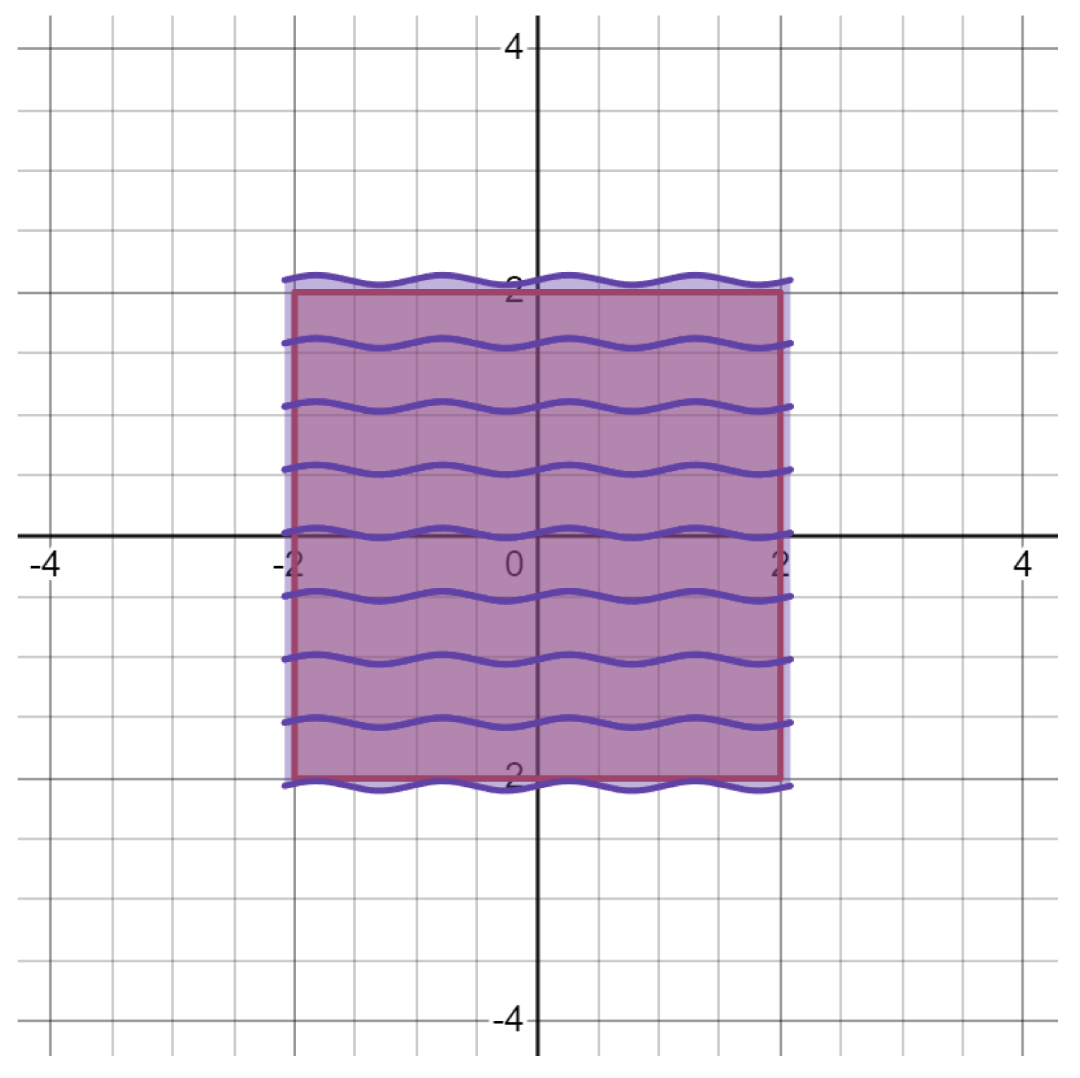
Suppose

• $A={\mathbb{R}}^2$
• ${\left(F_r^{★}\right)}_{r\in \mathbb{N}}={\left([-r,r]\times [-r,r]\right)}_{r\in \mathbb{N}}$

Then one example of $\mathbf{C}(13/6,F_2^{★},1)$, using §5.4.1 step 1, (where $F_2^{★}=[-2,2]\times [-2,2]$) is:

$$\begin{array}{cccc}& \{\hfill & & \left[-\sqrt{{\displaystyle \frac{13}{3}}},\sqrt{{\displaystyle \frac{13}{3}}}\right]\times \left[-\sqrt{{\displaystyle \frac{13}{3}}},-{\displaystyle \frac{3}{4}}\sqrt{{\displaystyle \frac{13}{3}}}\right),\left[-\sqrt{{\displaystyle \frac{13}{3}}},\sqrt{{\displaystyle \frac{13}{3}}}\right]\times \left[-{\displaystyle \frac{3}{4}}\sqrt{{\displaystyle \frac{13}{3}}},-{\displaystyle \frac{1}{2}}\sqrt{{\displaystyle \frac{13}{3}}}\right),\left[-\sqrt{{\displaystyle \frac{13}{3}}},\sqrt{{\displaystyle \frac{13}{3}}}\right]\times \left[-{\displaystyle \frac{1}{2}}\sqrt{{\displaystyle \frac{13}{3}}},-{\displaystyle \frac{1}{4}}\sqrt{{\displaystyle \frac{13}{3}}}\right),\hfill \\ & & & \left[-\sqrt{{\displaystyle \frac{13}{3}}},\sqrt{{\displaystyle \frac{13}{3}}}\right]\times \left[-{\displaystyle \frac{1}{4}}\sqrt{{\displaystyle \frac{13}{3}}},0\right),\left[-\sqrt{{\displaystyle \frac{13}{3}}},\sqrt{{\displaystyle \frac{13}{3}}}\right]\times \left[0,{\displaystyle \frac{1}{4}}\sqrt{{\displaystyle \frac{13}{3}}}\right),\left[-\sqrt{{\displaystyle \frac{13}{3}}},\sqrt{{\displaystyle \frac{13}{3}}}\right]\times \left[{\displaystyle \frac{1}{4}}\sqrt{{\displaystyle \frac{13}{3}}},{\displaystyle \frac{1}{2}}\sqrt{{\displaystyle \frac{13}{3}}}\right),\hfill \\ & & & \left[-\sqrt{{\displaystyle \frac{13}{3}}},\sqrt{{\displaystyle \frac{13}{3}}}\right]\times \left[{\displaystyle \frac{1}{2}}\sqrt{{\displaystyle \frac{13}{3}}},{\displaystyle \frac{3}{4}}\sqrt{{\displaystyle \frac{13}{3}}}\right),\left[-\sqrt{{\displaystyle \frac{13}{3}}},\sqrt{{\displaystyle \frac{13}{3}}}\right]\times \left[{\displaystyle \frac{3}{4}}\sqrt{{\displaystyle \frac{13}{3}}},\sqrt{{\displaystyle \frac{13}{3}}}\right]\}\hfill \end{array}$$

(14)

Note, the area of each of the rectangles is $13/6$, where the borders could be approximated as:

$$\begin{array}{c}\{\left[-2.082,2.082\right]\times \left[-2.082,-1.561\right),\left[-2.082,2.082\right]\times \left[-1.561,-1.041\right),\left[-2.082,2.082\right]\times \left[-1.041,-.520\right),\hfill \\ \left[-2.082,2.082\right]\times \left[-.520,0\right),\left[-2.082,2.082\right]\times \left[0,.520\right),\left[-2.082,2.082\right]\times \left[.520,1.041\right),\hfill \\ \left[-2.082,2.082\right]\times \left[1.041,1.561\right),\left[-2.082,2.082\right]\times \left[1.561,2.082\right]\}\hfill \end{array}$$

(15)

and we’ll illustrate this as purple rectangles covering $F_2^{★}$ (i.e., the red square).

(Note, the purple rectangles in Figure 1, satisfy step (1) of §5.4.1, since the Hausdorff measures in its dimension of the rectangles is $13/6$ and there is a minimum 8 covers over-covering $F_2^{★}$: i.e.,

Definition 3.

[Minimum Covers of Measure $\epsilon$ covering $F_r^{★}$] We can compute the minimum covers $\mathbf{C}(\epsilon ,F_r^{★},\omega )$, using the formula:

$$\lceil {\mathcal{H}}^{{\dim }_{\mathrm{H}}\left(F_r^{★}\right)}\left(F_r^{★}\right)/\epsilon \rceil$$

where $\lceil {\mathcal{H}}^{{\dim }_{\mathrm{H}}\left(F_2^{★}\right)}\left(F_2^{★}\right)/\epsilon \rceil =\lceil \mathrm{Area}\left({[-2,2]}^2\right)/(13/6)\rceil =\lceil 16/(13/6)\rceil =\lceil 96/13\rceil =\lceil 7+(5/13)\rceil =8$)

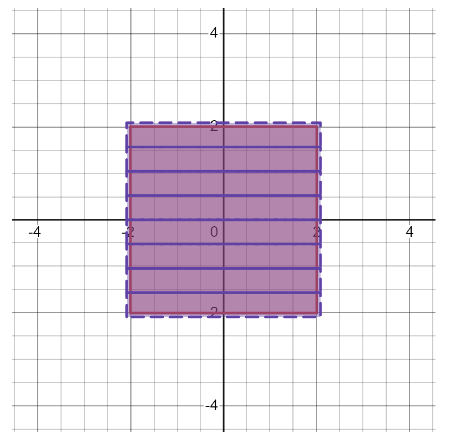
Note the covers in $\mathbf{C}(13/6,F_r^{★},\omega )$ need not be rectangles. In fact, they could be any set as long as the “area" of those sets is $13/6$, and $F_2^{★}$ is over-covered by the smallest number of sets possible. Here is an example:

Figure 2. The eight purple sets are the “covers" and the red square is $F_2^{★}$. (Ignore the boundaries)

Figure 2. The eight purple sets are the “covers" and the red square is $F_2^{★}$. (Ignore the boundaries)

To define this cover, start off with:

$$\begin{array}{c}{B}_1\left(x\right)=-2.062+.04sin\left(6.037x\right)\end{array}$$

(16)

$$\begin{array}{c}{B}_2\left(x\right)=-1.541+.04sin\left(6.037x\right)\end{array}$$

(17)

$$\begin{array}{c}{B}_3\left(x\right)=-1.021+.04sin\left(6.037x\right)\end{array}$$

(18)

$$\begin{array}{c}{B}_4\left(x\right)=-0.500+.04sin\left(6.037x\right)\end{array}$$

(19)

$$\begin{array}{c}{B}_5\left(x\right)=0.020+.04sin\left(6.037x\right)\end{array}$$

(20)

$$\begin{array}{c}{B}_6\left(x\right)=0.540+.04sin\left(6.037x\right)\end{array}$$

(21)

$$\begin{array}{c}{B}_7\left(x\right)=1.061+.04sin\left(6.037x\right)\end{array}$$

(22)

$$\begin{array}{c}{B}_8\left(x\right)=1.581+.04sin\left(6.037x\right)\end{array}$$

(23)

$$\begin{array}{c}{B}_9\left(x\right)=2.102+.04sin\left(6.037x\right)\end{array}$$

(24)

Then, for each $i\in \mathbb{N}$ in $1\le i\le 7$, we define:

$${\mathcal{B}}_i=\left\{(x,y):-2.082\le x\le 2.082,B_i\left(x\right)\le y<B_{i+1}\left(x\right)\right\}$$

except $i=8$ where:

$${\mathcal{B}}_8=\left\{(x,y):-2.082\le x\le 2.082,B_8\left(x\right)\le y\le B_9\left(x\right)\right\}$$

such that an example of $\mathbf{C}(13/6,F_2^{★},2)$ is:

$$\{{\mathcal{B}}_1,{\mathcal{B}}_2,{\mathcal{B}}_3,{\mathcal{B}}_4,{\mathcal{B}}_5,{\mathcal{B}}_6,{\mathcal{B}}_7,{\mathcal{B}}_8\}$$

(26)

In the case of $F_2^{★}$, there are uncountably many $\mathbf{C}(13/6,F_2^{★},\omega )$ of different shapes and sizes which we can use. However, these examples were the ones taken.

8.2. Example of §5.4.1, step 2

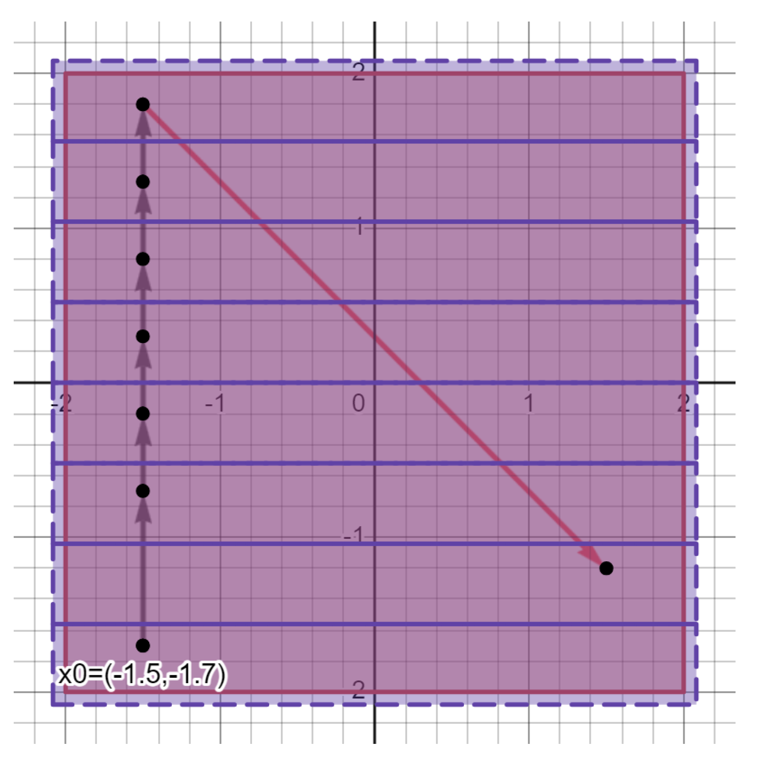
Suppose

• $A={\mathbb{R}}^2$
• ${\left(F_r^{★}\right)}_{r\in \mathbb{N}}={\left([-r,r]\times [-r,r]\right)}_{r\in \mathbb{N}}$
• $F_2^{★}=[-2,2]\times [-2,2]$
• $\mathbf{C}(13/6,F_2^{★},3)$, using Equation (15) and Figure 1, is

  $$\begin{array}{cccc}& \{\hfill & & \left[-2.082,2.082\right]\times \left[-2.082,-1.561\right),\left[-2.082,2.082\right]\times \left[-1.561,-1.041\right),\left[-2.082,2.082\right]\times \left[-1.041,-.520\right),\hfill \\ & & & \left[-2.082,2.082\right]\times \left[-.520,0\right),\left[-2.082,2.082\right]\times \left[0,.520\right),\left[-2.082,2.082\right]\times \left[.520,1.041\right),\hfill \\ & & & \left[-2.082,2.082\right]\times \left[1.041,1.561\right),\left[-2.082,2.082\right]\times \left[1.561,2.082\right]\}\hfill \end{array}$$

  (27)

Then, an example of $\mathcal{S}(\mathbf{C}(13/6,F_2^{★},3),1)$ is:

$$\left\{\right(-1.5,-1.7),(1.5,-1.2),(-1.5,-.7),(-1.5,-.2),(-1.5,.3),(-1.5,.8),(-1.5,1.3),(-1.5,1.8\left)\right\}$$

(28)

Below, is an illustration of the sample: i.e., the set of all black points in each purple rectangle of $\mathbf{C}(13/6,F_2^{★},3)$ covering $F_2^{★}={[-2,2]}^2$:

Figure 3. The black points are the “sample points", the eight purple rectangles are the “covers", and the red square is $F_2^{★}$. (Ignore the boundaries)

Figure 3. The black points are the “sample points", the eight purple rectangles are the “covers", and the red square is $F_2^{★}$. (Ignore the boundaries)

Note there are multiple samples we can take, as long as one sample point is taken from each cover in $\mathbf{C}(13/6,F_2^{★},1)$.

8.3. Example of §5.4.1, step 3

Suppose

• $A={\mathbb{R}}^2$
• ${\left(F_r^{★}\right)}_{r\in \mathbb{N}}={\left([-r,r]\times [-r,r]\right)}_{r\in \mathbb{N}}$
• $F_2^{★}=[-2,2]\times [-2,2]$
• $\mathbf{C}(13/6,F_2^{★},3)$, using Equation (15) and Figure 1, is

  $$\begin{array}{cccc}& \{\hfill & & \left[-2.082,2.082\right]\times \left[-2.082,-1.561\right),\left[-2.082,2.082\right]\times \left[-1.561,-1.041\right),\left[-2.082,2.082\right]\times \left[-1.041,-.520\right),\hfill \\ & & & \left[-2.082,2.082\right]\times \left[-.520,0\right),\left[-2.082,2.082\right]\times \left[0,.520\right),\left[-2.082,2.082\right]\times \left[.520,1.041\right),\hfill \\ & & & \left[-2.082,2.082\right]\times \left[1.041,1.561\right),\left[-2.082,2.082\right]\times \left[1.561,2.082\right]\}\hfill \end{array}$$
• $\mathcal{S}(\mathbf{C}(13/6,F_2^{★},3),1)$, using Equation (28), is:

  $$\left\{\right(-1.5,-1.7),(1.5,-1.2),(-1.5,-.7),(-1.5,-.2),(-1.5,.3),(-1.5,.8),(-1.5,1.3),(-1.5,1.8\left)\right\}$$

  (29)

Therefore, consider the following process:

8.3.1. Step 33a

If $\mathcal{S}(\mathbf{C}(13/6,F_2^{★},3),1)$ is:

$$\left\{\right(-1.5,-1.7),(1.5,-1.2),(-1.5,-.7),(-1.5,-.2),(-1.5,.3),(-1.5,.8),(-1.5,1.3),(-1.5,1.8\left)\right\}$$

(30)

suppose $x_0=(-1.5,-1.7)$. Note, the following:

• $x_1=(-1.5,-.7)$ is the next point in the “pathway" since it’s a point in $\mathcal{S}(\mathbf{C}(13/6,F_2^{★},3),1)$ with the smallest 2-d Euclidean distance to $x_0$ instead of $x_0$.
• $x_2=(-1.5,-.2)$ is the third point since it’s a point in $\mathcal{S}(\mathbf{C}(13/6,F_2^{★},3),1)$ with the smallest 2-d Euclidean distance to $x_1$ instead of $x_0$ and $x_1$.
• $x_3=(-1.5,.3)$ is the fourth point since it’s a point in $\mathcal{S}(\mathbf{C}(13/6,F_2^{★},3),1)$ with the smallest 2-d Euclidean distance to $x_2$ instead of $x_0$, $x_1$, and $x_2$.
• we continue this process, where the “pathway" of $\mathcal{S}(\mathbf{C}(13/6,F_2^{★},3),1)$ is:

$$(-1.5,-1.7)\to (-1.5,-.7)\to (-1.5,-.2)\to (-1.5,.3)\to (-1.5,.8)\to (-1.5,1.3)\to (-1.5,1.8)\to (1.5,-1.2)$$

(31)

Note 3. If more than one point has the minimum 2-d Euclidean distance from $x_0$, $x_1$, $x_2$, etc. take all potential pathways: e.g., using the sample in Equation (30), if $x_0=(-1.5,-.2)$, then since $(-1.5,-.7)$ and $(-1.5,.3)$ have the smallest Euclidean distance from $(-1.5,-.2)$, and for point $x_1=(-1.5,-.7)$, since $(-1.5,-1.7)$ and $(-1.5,.3)$ have the smallest Euclidean distance from $(-1.5,-.7)$, we take three pathways:

$$\begin{array}{c}(-1.5,-.2)\to (-1.5,-.7)\to (-1.5,-1.7)\to (-1.5,.3)\to (-1.5,.8)\to (-1.5,1.3)\to (-1.5,1.8)\to (1.5,-1.2)\\ (-1.5,-.2)\to (-1.5,-.7)\to (-1.5,.3)\to (-1.5,.8)\to (-1.5,1.3)\to (-1.5,1.8)\to (-1.5,-1.7)\to (1.5,-1.2)\\ (-1.5,-.2)\to (-1.5,.3)\to (-1.5,.8)\to (-1.5,1.3)\to (-1.5,1.8)\to (-1.5,-.7)\to (-1.5,-1.7)\to (1.5,-1.2)\end{array}$$

8.3.2. Step 33b

Take the length of all line segments in the pathway. In other words, suppose $d(P,Q)$ is the n-th dim.Euclidean distance between points $P,Q\in {\mathbb{R}}^n$. Using the pathway of eq. 31, we want:

$$\begin{array}{cc}\hfill \{& d\left(\right(-1.5,-1.7),(-1.5,-.7\left)\right),d\left(\right(-1.5,-.7),(-1.5,-.2\left)\right),d\left(\right(-1.5,-.2),(-1.5,.3\left)\right),d\left(\right(-1.5,.3),(-1.5,.8\left)\right),\hfill \\ & d\left(\right(-1.5,.8),(-1.5,1.3\left)\right),d\left(\right(-1.5,1.3),(-1.5,1.8\left)\right),d\left(\right(-1.5,1.8),(1.5,-1.2\left)\right)\}\hfill \end{array}$$

(32)

Whose distances can be approximated as:

$$\begin{array}{cc}\hfill \{& 1,.5,.5,.5,.5,.5,4.25\}\hfill \end{array}$$

(33)

As we can see, the outlier [8] is $4.25$ (i.e., note these outliers become more prominent for $\epsilon \ll 13/6$). Therefore, remove $4.25$ from the set of distances:

$$\begin{array}{cc}\hfill \{& 1,.5,.5,.5,.5,.5\}\hfill \end{array}$$

which we can illustrate with:

Figure 4. $x_0$ is the start point in the pathway. The black line segments in the “pathway" have lengths which aren’t outliers. The length of the red line segment is an outlier.

Figure 4. $x_0$ is the start point in the pathway. The black line segments in the “pathway" have lengths which aren’t outliers. The length of the red line segment is an outlier.

Hence, when $x_0=(-1.5,-1.7)$, using §5.4.1 step 33b & Equation (30, we note:

$$\mathcal{L}((-1.5,-1.7),\mathcal{S}(\mathbf{C}(13/6,F_2^{★},3),1))=\{1,.5,.5,.5,.5,.5\}$$

(34)

8.3.3. Step 33c

To convert the set of distances in Equation (34) into a probability distribution, we take:

$$\sum _{x\in \{1,.5,.5,.5,.5,.5\}}x=1+.5+.5+.5+.5+.5=3.5$$

(35)

Then divide each element in $\{1,.5,.5,.5,.5,.5\}$ by 3.5

$$\{1/(3.5),.5/(3.5),.5/(3.5),.5/(3.5),.5/(3.5),.5/(3.5\left)\right\}$$

which gives us the probability distribution:

$$\{2/7,1/7,1/7,1/7,1/7,1/7\}$$

Hence,

$$\mathbb{P}\left(\mathcal{L}((-1.5,-1.7),\mathcal{S}(\mathbf{C}(\epsilon ,F_2^{★},3),1))\right)=\{2/7,1/7,1/7,1/7,1/7,1/7\}$$

(36)

8.3.4. Step 33d

Take the shannon entropy of Equation (36):

$$\begin{array}{cc}\hfill & \mathrm{E}\left(\mathbb{P}\left(\mathcal{L}((-1.5,-1.7),\mathcal{S}(\mathbf{C}(13/6,F_2^{★},1),3))\right)\right)=\hfill \\ & \sum _{x\in \mathbb{P}\left(\mathcal{L}((-1.5,-1.7),\mathcal{S}(\mathbf{C}(13/6,F_r,\omega ),\psi ))\right)}-x{log}_{2}x=\sum _{x\in \{2/7,1/7,1/7,1/7,1/7,1/7\}}-x{log}_{2}x=\hfill \\ & -(2/7){log}_2(2/7)-(1/7){log}_2(1/7)-(1/7){log}_2(1/7)-(1/7){log}_2(1/7)-(1/7){log}_2(1/7)-(1/7){log}_2(1/7)=\hfill \\ & -(2/7){log}_2(2/7)-(5/7){log}_2(1/7)\approx 2.5216\hfill \end{array}$$

We shorten $\mathrm{E}\left(\mathbb{P}\left(\mathcal{L}((-1.5,-1.7),\mathcal{S}(\mathbf{C}(13/6,F_2^{★},3),1))\right)\right)$ to $\mathrm{E}\left(\mathcal{L}((-1.5,-1.7),\mathcal{S}(\mathbf{C}(13/6,F_2^{★},3),1))\right)$, giving us:

$$\mathrm{E}\left(\mathcal{L}((-1.5,-1.7),\mathcal{S}(\mathbf{C}(13/6,F_2^{★},3),1))\right)\approx 2.5216$$

(37)

8.3.5. Step 33e

Take the entropy w.r.t all pathways of:

$$\begin{array}{cc}\hfill & \mathcal{S}(\mathbf{C}(13/6,F_2^{★},1),3)\left)\right)=\hfill \\ \hfill & \left\{\right(-1.5,-1.7),(1.5,-1.2),(-1.5,-.7),(-1.5,-.2),(-1.5,.3),(-1.5,.8),(-1.5,1.3),(-1.5,1.8\left)\right\}\hfill \end{array}$$

In other words, we’ll compute:

$$\mathrm{E}\left(\mathcal{L}\left(\mathcal{S}(\mathbf{C}(13/6,F_2^{★},3),1)\right)\right)=\underset{x_0\in \mathcal{S}(\mathbf{C}(13/6,F_2^{★},3),1)}{sup}\mathrm{E}\left(\mathcal{L}(x_0,\mathcal{S}(\mathbf{C}(13/6,F_2^{★},3),1))\right)$$

We do this by repeating §8.3.1-§8.3.4 for different $x_0\in \mathcal{S}(\mathbf{C}(13/6,F_2^{★},1),3)\left)\right)$ (i.e., in the equations with multiple values, see Note 5)

$$\begin{array}{cc}\hfill & \mathrm{E}\left(\mathcal{L}((-1.5,-1.7),\mathcal{S}(\mathbf{C}(13/6,F_2^{★},3),1))\right)\approx 2.52164\hfill \end{array}$$

(38)

$$\begin{array}{cc}\hfill & \mathrm{E}\left(\mathcal{L}((1.5,-1.2),\mathcal{S}(\mathbf{C}(13/6,F_2^{★},3),1))\right)\approx 2.34567\hfill \end{array}$$

(39)

$$\begin{array}{cc}\hfill & \mathrm{E}\left(\mathcal{L}((-1.5,-0.7),\mathcal{S}(\mathbf{C}(13/6,F_2^{★},3),1))\right)\approx 2.2136\hfill \end{array}$$

(40)

$$\begin{array}{cc}\hfill & \mathrm{E}\left(\mathcal{L}((-1.5,-0.2),\mathcal{S}(\mathbf{C}(13/6,F_2^{★},3),1))\right)\approx 2.32193,2.11807,2.3703\hfill \end{array}$$

(41)

$$\begin{array}{cc}\hfill & \mathrm{E}\left(\mathcal{L}((-1.5,0.3),\mathcal{S}(\mathbf{C}(13/6,F_2^{★},3),1))\right)\approx 2.24244,2.40051\hfill \end{array}$$

(42)

$$\begin{array}{cc}\hfill & \mathrm{E}\left(\mathcal{L}((-1.5,0.8),\mathcal{S}(\mathbf{C}(13/6,F_2^{★},3),1))\right)\approx 2.22393,2.41651\hfill \end{array}$$

(43)

$$\begin{array}{cc}\hfill & \mathrm{E}\left(\mathcal{L}((-1.5,1.3),\mathcal{S}(\mathbf{C}(13/6,F_2^{★},3),1))\right)\approx 2.22208,2.4076\hfill \end{array}$$

(44)

$$\begin{array}{cc}\hfill & \mathrm{E}\left(\mathcal{L}((-1.5,1.8),\mathcal{S}(\mathbf{C}(13/6,F_2^{★},3),1))\right)\approx 2.52164\hfill \end{array}$$

(45)

Hence, since the largest value out of Equations (38)–(45) is 2.52164:

$$\mathrm{E}\left(\mathcal{L}\left(\mathcal{S}(\mathbf{C}(13/6,F_2^{★},3),1)\right)\right)=\underset{x_0\in \mathcal{S}(\mathbf{C}(\epsilon ,F_2^{★},3),1)}{sup}\mathrm{E}\left(\mathcal{L}(x_0,\mathcal{S}(\mathbf{C}(\epsilon ,F_2^{★},3),1))\right)\approx 2.52164$$

References

- Achour, R.; Li, Z.; Selmi, B.; Wang, T. A multifractal formalism for new general fractal measures. Chaos, Solitons & Fractals 2024, 181, 114655. [Google Scholar]
- Bedford, T.; Fisher, A.M. Analogues of the Lebesgue density theorem for fractal sets of reals and integers. Proceedings of the London Mathematical Society 1992, 3, 95–124. [Google Scholar] [CrossRef]
- Bedford, T.; Fisher, A.M. Ratio geometry, rigidity and the scenery process for hyperbolic Cantor sets. Ergodic Theory and Dynamical Systems 1997, 17, 531–564. [Google Scholar] [CrossRef]
- Sipser, M. Introduction to the Theory of Computation, 3 ed.; Cengage Learning, 2012; pp. 275–322. [Google Scholar]
- Krishnan, B. Bharath Krishnan’s ResearchGate Profile. https://www.researchgate.net/profile/Bharath-Krishnan-4.
- Barański, K.; Gutman, Y.; Śpiewak, A. Prediction of dynamical systems from time-delayed measurements with self-intersections. Journal de Mathématiques Pures et Appliquées 2024, 186, 103–149. [Google Scholar] [CrossRef]
- Caetano, A.M.; Chandler-Wilde, S.N.; Gibbs, A.; Hewett, D.P.; Moiola, A. A Hausdorff-measure boundary element method for acoustic scattering by fractal screens. Numerische Mathematik 2024, 156, 463–532. [Google Scholar] [CrossRef]
- John, R. Outlier. https://en.m.wikipedia.org/wiki/Outlier.
- M., G. Entropy and Information Theory, 2 ed.; Springer New York: New York [America];, 2011; pp. 61–95. https://ee.stanford.edu/~gray/it.pdf. [CrossRef]
Figure 1.
Purple rectangles are the “covers" and the red square is . (Ignore the boundaries)
Disclaimer/Publisher’s Note: The statements, opinions and data contained in all publications are solely those of the individual author(s) and contributor(s) and not of MDPI and/or the editor(s). MDPI and/or the editor(s) disclaim responsibility for any injury to people or property resulting from any ideas, methods, instructions or products referred to in the content. |
© 2024 by the authors. Licensee MDPI, Basel, Switzerland. This article is an open access article distributed under the terms and conditions of the Creative Commons Attribution (CC BY) license (http://creativecommons.org/licenses/by/4.0/).
Copyright: This open access article is published under a Creative Commons CC BY 4.0 license, which permit the free download, distribution, and reuse, provided that the author and preprint are cited in any reuse.