
Submitted:
20 February 2025
Posted:
27 February 2025
You are already at the latest version
Abstract
Suppose n ∈ N. We wish to meaningfully average ‘sophisticated’ unbounded sets (i.e., sets with positive n-d Hausdorff measure, in any n-d box of the n-d plane, where the measures do not equal the area of the boxes). We do this by taking an unique, satisfying extension of the expected value, w.r.t the Hausdorff measure in its dimension, on bounded sets taking finite values only. As of now, I’m unable to define this due to limited knowledge of advanced math and most people are too busy to help. Therefore, I’m wondering if anyone knows a research paper which solves my doubts. (Unlike previous versions with similar names, we made everything rigorous.)
Keywords:
Expected Values
; Sets
; Hausdorff measure
; Hausdorff dimension
; Discretization
; Segmentation
; Partitions
; Samples
; Euclidean Distance
; Choice Function
1. Intro
Let . Suppose is Borel, where:
- is the set of all unbounded Borel subsets of a set
- is the set of all bounded Borel subsets of a set
In addition, is the Hausdorff dimension and is the Hausdorff measure in its dimension on the Borel -algebra.
1.1. First Special Case of A
Suppose the n-dimensional box is B. We want an explicitA, such that:
- (1)
- for all B
- (2)
- for all B.
This case of A is called .
1.1.1. Potential Answer
If , using this reddit post [1], define A such that:
Find some set , where for every interval I.
Hence, construct a subset of with this property (then copy and paste this set to get the desired set ):
We do this by constructing a strange map from . Take a real number , expand that number in binary as and map the value to the series . It’s possible using Khintchine’s inequality [2] to show the sum converges for a.e. . Thus, our desired set will just consist of those x for which the sum is positive.
The fact this set works is a little bit annoying to prove, but relies on Khintchine’s inequality [2 p.187-205] and the divergence of the Harmonic series. Essentially, we want to show that for any initial seqeuence of digits there is a positive probability that the final sum is positive and a positive probability that the final sum is negative.
Note, in case there is a research paper which can average into a finite number, consider the next example.
1.2. Second Special Case of A
Suppose the n-dimensional box is B. Is there an explicit A, such that:
- 1.
- for all B
- 2.
- for all B
- 3.
-
For all n-d boxes :
- (a)
- (b)
- (c)
- ?
If explicit A exists, what is an example? If not, how does one modify , so that it exists?
If such a set exists, this case of A is called . (We have yet to prove or disprove exists.)
1.3. Attempting to Analyze/Average A
The expected value of A, w.r.t the Hausdorff measure in its dimension, is:
Nevertheless, we have the following problems:
Notation 1
(Problem 1). When 1.1), is undefined.
1.3.1. Explanation of Problem 1
When , using Section 1.1 and Section 1.1.1, since for all B, notice and . This makes undefined due to division by infinity. Similarly, the most obvious extension of or is also undefined; i.e., given the absolute value is , then the following is false since for all B:
Notation 2
(Problem 2). Suppose is the set of all unbounded Borel subsets of and is the n-d Euclidean norm. If is the set of all , where is finite and the cardinality is , then (i.e., is “measure zero" in )
1.3.2. Explanation of Problem 2
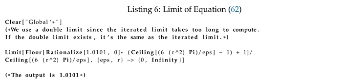
All unbounded A have means with a finite n-d norm when the symmetry lines of A intersect at one point. Thus, for any sequence of bounded sets whose set-theoretic limit (Section 1.3.3) is A, such that the lines of symmetry of A intersect at one point, in the following statement ( is the absolute value):
always exists and has the same value.
Since the cardinality of the set of all unbounded sets with one or more symmetry lines is , the cardinality of all unbounded sets whose lines of symmetry intersect at one point is less than or equal to . Hence, since the cardinality of the collection of all unbounded subsets of is , and . Thus, we conclude , which shows problem 2 is correct.
Therefore, suppose:
1.3.3. Set Theoretic Limit of a Sequence of Sets
The set-theoretic limit of a sequence of sets of bounded set is A when:
where:
which we represent with the notation:
Now, consider an approach to solving problems and :
1.3.4. Approach
Suppose is the set of all unbounded Borel subsets of and is the set of all bounded Borel subsets of , where is an arbitrary set. In addition, suppose is the n-d Euclidean norm. If is the set of all , where for all and , such that (Section 1.3.3), is unique, is satisfying (Section 3), and is finite:
- 1.
- (i.e., is “almost everywhere" in )
- 2.
- If (1) isn’t true, then
1.3.5. Explanation of Approach
If (Section 1.3.3) where we apply (Section 1.3.2 Equation (2), depending on the chosen, could be one of many values. Here is an example:
Example 1.
Suppose . We define the bounded sequences of sets and , where 1.3.3). Note, the center of , for all , is and the center of , for all , is . Thus, and . Furthermore, depending on the chosen, can be any point in (when it exists).
Therefore, we ask the following:
1.4. Question
Is there a unique way to define “satisfying" in the approach of , which solves problems 1 and 2 with applications?
2. Extending the Expected Value of A w.r.t the Hausdorff Measure
The following are two methods to finding the most generalized, satisfying extension of in Equation (1) which we later use to answer the question in :
- One way is defining a generalized, satisfying extension of the Hausdorff measure, on all A with positive & finite measure which takes positive, finite values for all Borel A. This can theoretically be done in the paper “A Multi-Fractal Formalism for New General Fractal Measures"[3], where in Equation 1 we replace the Hausdorff measure with the extended Hausdorff measure.
- Another way is finding generalized, satisfying average of all A in the fractal setting. This can be done with the papers “Analogues of the Lebesgue Density Theorem for Fractal Sets of Reals and Integers" [4] and “Ratio Geometry, Rigidity and the Scenery Process for Hyperbolic Cantor Sets" [5] where we take the expected value of A w.r.t the densities in [4,5].
Note, neither approach answers Section 1.4, since the n-d norms of the averages in the approach are not unique for unbounded sets (ex. 1). Therefore, we ask a leading question that uses to guide readers to an interesting solution to Section 1.4.
3. Attempt to Define “Unique and Satisfying" in The Approach of Section 1.3
3.1. Leading Question
To define satisfying inside the approach of Section 1.3.4, we take the expected value of a sequence of bounded sets chosen by a choice function. To find the choice function, we ask the leading question...
Suppose is the set of all bounded Borel subsets of , where there exists an arbitrary set , such that for all :
- (A)
- (B)
- (C)
- □ is the logical symbol for “it’s necessary"
- (D)
- Define C to be chosen center point of (e.g., the origin)
- (E)
- Define E to be the fixed, expected rate of expansion of w.r.t center point C (e.g., )
- (F)
- Define to be actual rate of expansion of w.r.t center point C ( 5.5)
Does there exist a unique choice function which chooses an unique set , where for all , every is equivalent (Section 5.3, def. 1) to , such that:
- 1.
- 2.
- For all and , where (Section 1.3.3), the “measure" (Section 5.4.1, Section 5.4.2) of must increase at rate linear or superlinear to that of
- 3.
- If is the n-d Euclidean norm, is unique and is finite (Section 5.2).
- 4.
-
For some satisfying (1), (2), and (3), where for all , given , , and in (1), (2), and (3), s.t., note that for all , where satisfies (1), (2), and (3):
- If is the n-d Euclidean distance between , then
-
If , for any linear , where and the Big-O notation is , there exists a function , where the absolute value is and (Section 3.1.E-F):such that:In simpler terms, “the rate of divergence" of (Section 3.1.E-F) is less than or equal to “the rate of divergence" of (Section 3.1.E-F).
- 5.
-
If is the set of all unbounded Borel subsets of and is the set of all , where satisfies (1), (2), (3) and (4), then:
- (i.e., is “almost everywhere" in )
- When , replace the Hausdorff measure in of criteria (3) with the generalized measures and densities in , where we want
- When neither are possible, then
- 6.
- Out of all choice functions which satisfy (1), (2), (3), (4), and (5) we choose the one with the simplest form, meaning for each choice function fully expanded, we take the one with the fewest variables/numbers?
(In case this is unclear, see Section 5.)
I’m convinced , where all (Section 3.1) which answers the leading question isn’t unique nor satisfying enough to answer Section 1.3.4. Still, adjustments are possible by changing the criteria or by adding new criteria to 3.1.
4. Question Regarding My Work
Most don’t have time to address everything in my research, hence I ask the following:
Is there a research paper which already solves the ideas I’m working on? (Non-published papers, such as mine [6], don’t count.)
5. Clarifying Section 3
Let be an unbounded, Borel set. Suppose be the Hausdorff dimension and be the Hausdorff measure in its dimension on the Borel -algebra. See Section 3.1, once reading this section, and consider the following:
Is there a simpler version of the definitions below?
5.1. Set Theoretic Limit of a Sequence of Bounded Sets
Note, the set-theoretic limit of a sequence of sets of bounded set is A when:
where:
which we denote
Example 2.
When , we define sequences of sets and , such that . We aren’t sure how to prove this, but assume readers should be able to verify.
5.2. Expected Value of Bounded Sequences of Sets
If is a sequence of bounded sets, where (Section 5.1) and the absolute value is , the expected value of A w.r.t (when it exists) is a real number which satisfies the following:
Note, can be extended using Section 2.
5.2.1. Example 1
Using example 2, suppose , , and . Hence:
Since Equation (12) is true,
5.2.2. Example 2
Using example 2, suppose , , and . Hence:
Since Equation (24) is true, .
5.3. Defining Equivelant and Non-Equivelant Sequences of Bounded Functions
Definition 1
(Equivelant Sequences of Bounded Sets). The sequences of sets and are equivalent, if there exists , where for all , there exists , such that:
and for all , there exists , such that:
5.3.1. Explanation
Suppose is the set of all subsets of . Hence, and are equivalent, when for all sets , where (Section 5.1) and or exist, the following is true:
Thus, consider:
Theorem 1.
If and are equivalent, then for all , where :
Hence, consider the following:
5.3.2. Example of Equivalent Sequences of Bounded Sets
Suppose:
Now, suppose . Thus, using def. 1, we prove:
- 1.
-
For all , there exists a , where:which is proven with the following:
- 2.
-
For all , there exists a , where:which is proven with the following:
Since crit. and (2) is true, using definition 1, we have shown and are equivalent.
Note, there is no , where (), such that .
Definition 2
(Non-Equivalent Sequences of Bounded Sets). The sequences of sets and are non-equivalent, if there exists , where for all , there is either , such that:
or for all , there exists , such that:
5.3.3. Explanation
Suppose, is the set of all subsets of . Hence, and are non-equivalent, when there exists a set , where (Section 5.1) and or exist, s.t.the following is true:
Therefore, consider the following:
5.3.4. Example of Non-Equivalent Sequences of Bounded Sets
Suppose:
Now, suppose . Thus, using def. 2, we prove:
- 1.
-
For all , there exists a , where:which is proven using the following:Since is a 1-d interval, . Therefore:
Since crit. (1) is true, using definition 2, we have shown and are non-equivalent.
5.3.5. Question
When:
How do we find , where (Section 5.1), such that ( 5.2)?
5.4. Defining the “Measure"
5.4.1. Preliminaries
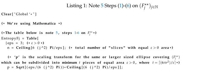
We define the “measure" of in . To understand this “measure", keep reading. (If the following steps are unclear, see Section 8 for examples.)
- 1.
- For every , “over-cover" with minimal, pairwise disjoint sets of equal measure. (We denote the equal measures , where the former sentence is defined : i.e., enumerates all collections of these sets covering . In case this step is unclear, see Appendix 8.1.)
- 2.
- For every , r and , take a sample point from each set in . The set of these points is “the sample" which we define : i.e., enumerates all possible samples of . (In the case this is unclear, see Sestion 8.2.)
- 3.
-
For every , r, and ,
- (a)
- Take a “pathway” of line segments: we start with a line segment from arbitrary point of to the sample point with smallest n-dimensional Euclidean distance to (i.e., when more than one sample point has smallest n-dimensional Euclidean distance to , take either of those points). Next, repeat this process until the “pathway” intersects with every sample point once. (If this is unclear, see Section 8.3.1.)
- (b)
- Take the set of the length of all segments in (3a), except for lengths that are outliers [7] (i.e., for any constant , the outliers are more than C times the interquartile range of the length of all line segments as ). Define this . (In case this is unclear, see Appendix 8.3.2.)
- (c)
- Multiply remaining lengths in the pathway by a constant so they add up to one (i.e., a probability distribution). This will be denoted . (In case this step is unclear, see Section 8.3.3.)
- (d)
- Take the shannon entropy [8, p.61-95] of step (3c). We define this:which will be shortened to . (In case this is unclear, see Section 8.3.4)
- (e)
- Maximize the entropy w.r.t all "pathways". This we will denote:
(In case this step is unclear, see Section 8.3.5.) - 4.
- Therefore, the maximum entropy of w.r.t , using (1) and (2) is:
5.4.2. What Am I Measuring?
Suppose we define two sequences of bounded sets that have a set theoretic limit of A: e.g., and , where for constant and cardinality
- (a)
- (b)
- 1.
- If using and we have:then what I’m measuring from increases at a rate superlinear to that of .
- 2.
- If using equations and (where we swap and , in and , with and ) we get:then what I’m measuring from increases at a rate sublinear to that of .
- 3.
-
If using equations , , , and , we both have:
- (a)
- or are equal to zero, one or
- (b)
- or are equal to zero, one or
then what I’m measuring from increases at a rate linear to that of .
Now consider the following examples:
5.4.3. Example of the “measure" of converging super-linearly to that of
Using Section 5.4.2 consider the following:
Notation 3.
Recall, if :
- When is the cardinality, for all and ,
-
For all and , the largest can be is
Now consider:
where:
Notation 4.
The area of and are:
Hence, we maximize by doing the following:
Notation 5
(Procedure to Maximize ). Consider the procedure below:
- 1.
- Cover the circle, with the same or larger-sized circle, which can be divided into minimum t “pie-slices" of equal area . Notice, .
- 2.
- Take the centroid of each slice
- 3.
- Out of all centroids in step 2, take the centroid with the largest x-coordinate: i.e., denote this point which is the start-point of the pathway of line segments in the resulting step
- 4.
- Take the distances between all pairs of consecutive centroids, starting with , rotating counter-clockwise or clockwise. Either-way, the end result should change by only a negligible amount.
- 5.
- Multiply the distances by a constant so they add up to 1 (i.e., a probability distribution)
- 6.
- Take the shannon entropy of the distribution using log base 2 in (33d)-(33e). (Note, since the “pie-slices" of step 1 are congruent and the distances of step 4 are equal, the entropy of the distribution is the largest possible amount (i.e., note 3 crit. 2 & note 4 crit. 1):
Repeat, steps 1-6 with , where the circle is an ellipse (i.e., with this case the “pie-slices" of step 1 are non-congruent and the distances of step 4 are non-equivelant). Hence, we use programming:
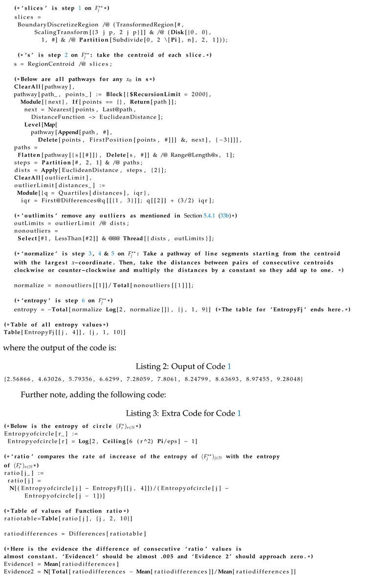
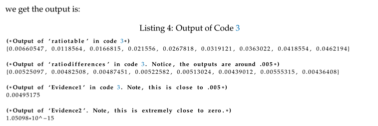
Note, the output of ratiotable in code 5 can be written as:
and is the same as:
Hence, with:
we solve for :
since:
Hence:
Note, using Section 5.4.2 (0a) and Section 5.4.2 (1), take and use note 3 crit. ii to compute the following:
where:
-
For every , we find a , where , but the absolute value of is minimized. In other words,for every , we want where:
Finally, since , we wish to prove
within Section 5.4.2 crit. 1:
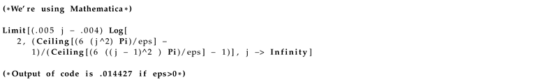
where using mathematica, we get the limit is greater than one:
- For every , we find a , where , but the absolute value of is minimized. In other words, for every , we want where:
Finally, since , we wish to prove
within Section 5.4.2 crit. 1:
where using mathematica, we get the limit is greater than one:
Hence, since the limits in Equation (61) and Equation (70) are greater than one and less than : i.e.,
we have proven what we’re measuring from increases at a rate superlinear to that of (i.e., Section 5.4.2 crit. 1).
5.4.4. Example of The “Measure" from Increasing at a Rate Sub-Linear to that of
Using our previous example, we can use the following theorem:
Theorem 2.
If what we’re measuring from increases at a rate superlinear to that of , then what we’re measuring from increases at a ratesublinearto that of
Hence, in our definition of super-linear (Section 5.4.2 crit. 1), swap and for and within and (i.e., and ). Notice, thm. 2 is true when:
5.4.5. Example of the “measure" of converging linearly to that of
Using Section 5.4.2 consider the following:
Notation 6.
Recall, if :
- When is the cardinality, for all and ,
-
For all and , the largest can be is
Now consider:
where:
Notation 7.
The area of and is:
Notice, since is a square, using note 6 crit. 2 and note 7 crit. 1, it’s simple to see:
Hence, using Section 5.4.2 (0b) and note 6 crit. (2):
Note, since is also a square, for all and
- For every , we find a , where , but the absolute value of is minimized. In other words, for every , we want where:
Hence Section 5.4.2 crit. 33a is true and then we prove Section 5.4.2 crit. 33b:
Note, since is a square, using note 6 crit. 2 and note 7 crit. 2, it’s simple to see:
Note, since is also a square, for all and
- For every , we find a , where , but the absolute value of is minimized. In other words, for every , we want a , where:
Hence:
and, using note 6 crit. 1 and note 6 crit. 1 with equation 92: . Thus, we wish to prove Section 5.4.2 crit. 33a using Equation( 93):
where Section 5.4.2 crit. 33b is true.
Therefore, since Section 5.4.2 crit. 3 is correct in this case, “the measure" of increases at a rate linear to that of
5.5. Defining The Actual Rate of Expansion of Sequence of Bounded Sets From C
In the next section, we will define the actual rate of expansion of sequence of bounded sets from C and give an example.
5.5.1. Definition of Actual Rate of Expansion of Sequence of Bounded Sets
Suppose is a bounded sequence of subsets of , and is the Euclidean distance between points . Therefore, using the “chosen" center point , when:
the actual rate of expansion is:
Note, there are cases of when isn’t fixed and (i.e., the fixed, expected rate of expansion).
5.5.2. Example
Suppose , , and . One can clearly see is the point on that is farthest from . Hence,
and the actual rate of expansion is:
5.6. Reminder
See if Section 3.1 is easier to understand?
6. My Attempt At Answering The Approach of Section 1.3
6.1. Choice Function
Suppose is the set of all bounded Borel subsets of . We then define the following:
- If is an arbitrary set, then for all , satisfies (1), (2), (3), (4), and (5) of the leading question in 3.1
- For all ,
Further note, from Section 5.4.2 (0b), if we take:
and from Section 5.4.2 (0b), we take:
then, using Section 5.4.1 (2), Equations (109) and (110):
6.2. Approach
We manipulate the definitions of Section 5.4.2 (0a), (0b) and Section 5.4.2 (ii) to solve 3.1 (1)-(5) of the leading question.
6.3. Potential Answer
6.3.1. Preliminaries (Definition of T)
Suppose:
- The average of for every is:
- is the n-d Euclidean distance between points
- The difference of point and is:
then define an explicit injective , where , such that:
- If , then
- If , then
- If , then
where:
6.3.2. Question
Does T exist? If so, how do we define it?
Thus, using , , , E, (Section 5.5), and with the absolute value function , ceiling function , and nearest integer function , we define:
the choice function, which answers the leading question in , could be the following, s.t.we explain the reason behind choosing the choice function in Section 6.4:
Theorem 3.
If we define:
where for , we define to be equivalent to when swapping “" with “" (for Equations (109) and (110)) and sets with (for Equation (109)–(116)), then for constant and variable , if:
and:
then for all ( crit. ii), if:
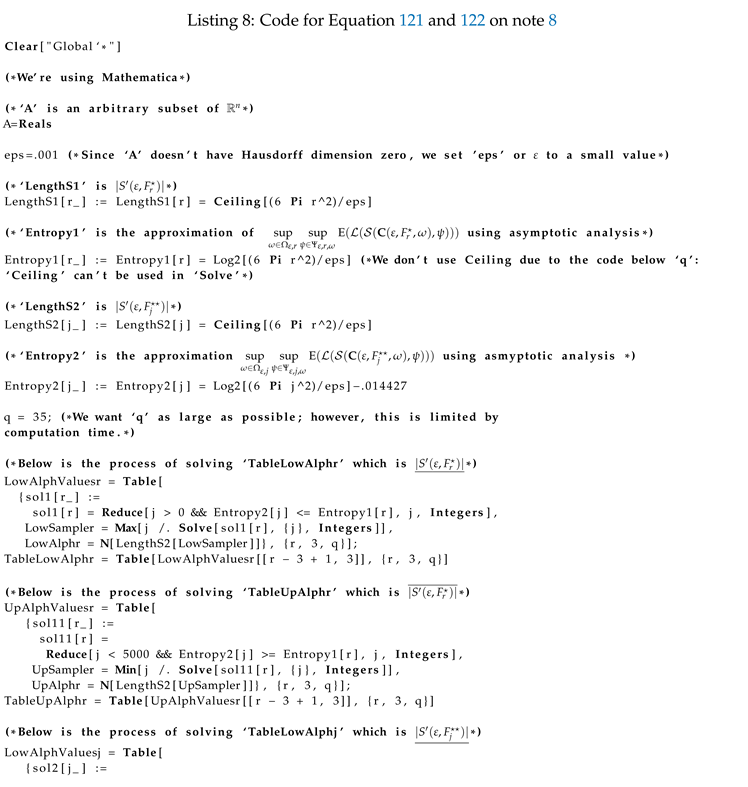
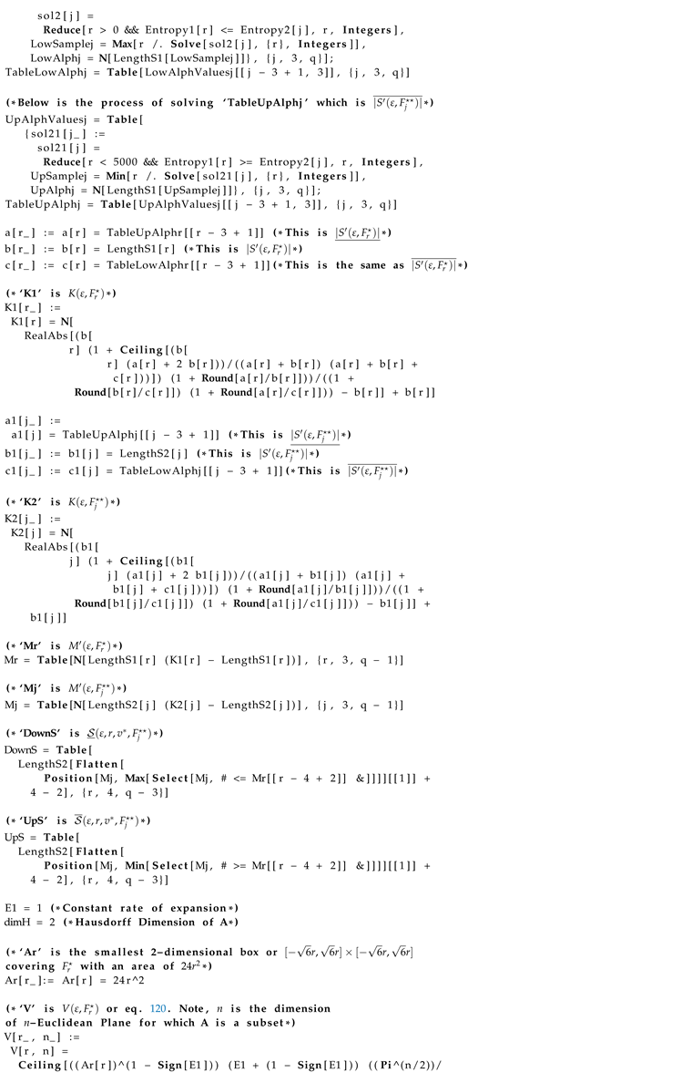
where is the ceiling function, E is the fixed rate of expansion, Γ is the gamma function, n is the dimension of , is the Hausdorff dimension of set , and is area of the smallest n-dimensional box that contains , then
the choice function is:
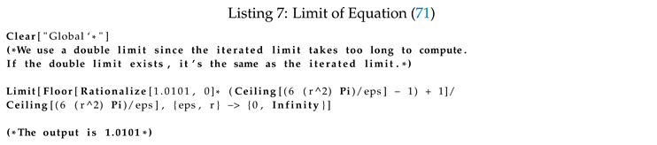
such that ( 6 crit. 2) must satisfy Equations (121) and (122). (Note, we want , , and to answer the leading question of ) where the answer to problems 1 and 2 & the approach of is (when it exists).
6.4. Explaining The Choice Function and Evidence The Choice Function Is Credible
Notice, before reading the programming in code , without the “c"-terms in Equation 121 and Equation 122:
- The choice function in Equation (121) and Equation (122) is zero, when what I’m measuring from (Section 5.4.2 criteria 1) increases at a rate superlinear to that of , where .
-
When c does exist, suppose:
- (a)
- When , then:
- (b)
- When , then:
Hence, for each sub-criteria under crit. (3), if we subtract one of their limits by their limit value, then Equation 121 and Equation (122) is zero. (We do this by using the “c"-term in Equations (121) and (122)). However, when the exponents of the “c"-terms aren’t equal to , the limits of Equation 121 and 122 aren’t equal to zero. We, infact, want this when we swap with . Moreover, we define function (i.e., Equation (120)), where:- i.
- ii.
- When then is zero, which makes Equation 121 and equal zero.
- iii.
-
Here are some examples of the numerator of (Equation (120)):
- A.
- When , , and , the numerator of is
- B.
- When , , and , the numerator of is
- C.
- When , , and , the numerator of is ceiling of constant times the volume of an n-dimensional ball with finite radius: i.e.,
- D.
- When , , and , the numerator of is ceiling of the volume of the n-dimensional ball: i.e.,
Notation 8.
Now, consider the code for Equation (121) and Equation (122). (Note, the set theoretic limit is set A. In this example, and:
We leave it to mathematicians to figure LengthS1, LengthS2, Entropy1 and for different A, , and .
7. Questions
- Does answer the in
- If is the n-d Euclidean norm, using and thm. 3, where , is unique and finite?
- If is the n-d Euclidean norm, using and thm. 3, where , is is unique and finite?
- If there’s no time to check questions 1, 2, and 3, see .
8. Appendix of Section 5.4.1
8.1. Example of Section 5.4.1, step 1
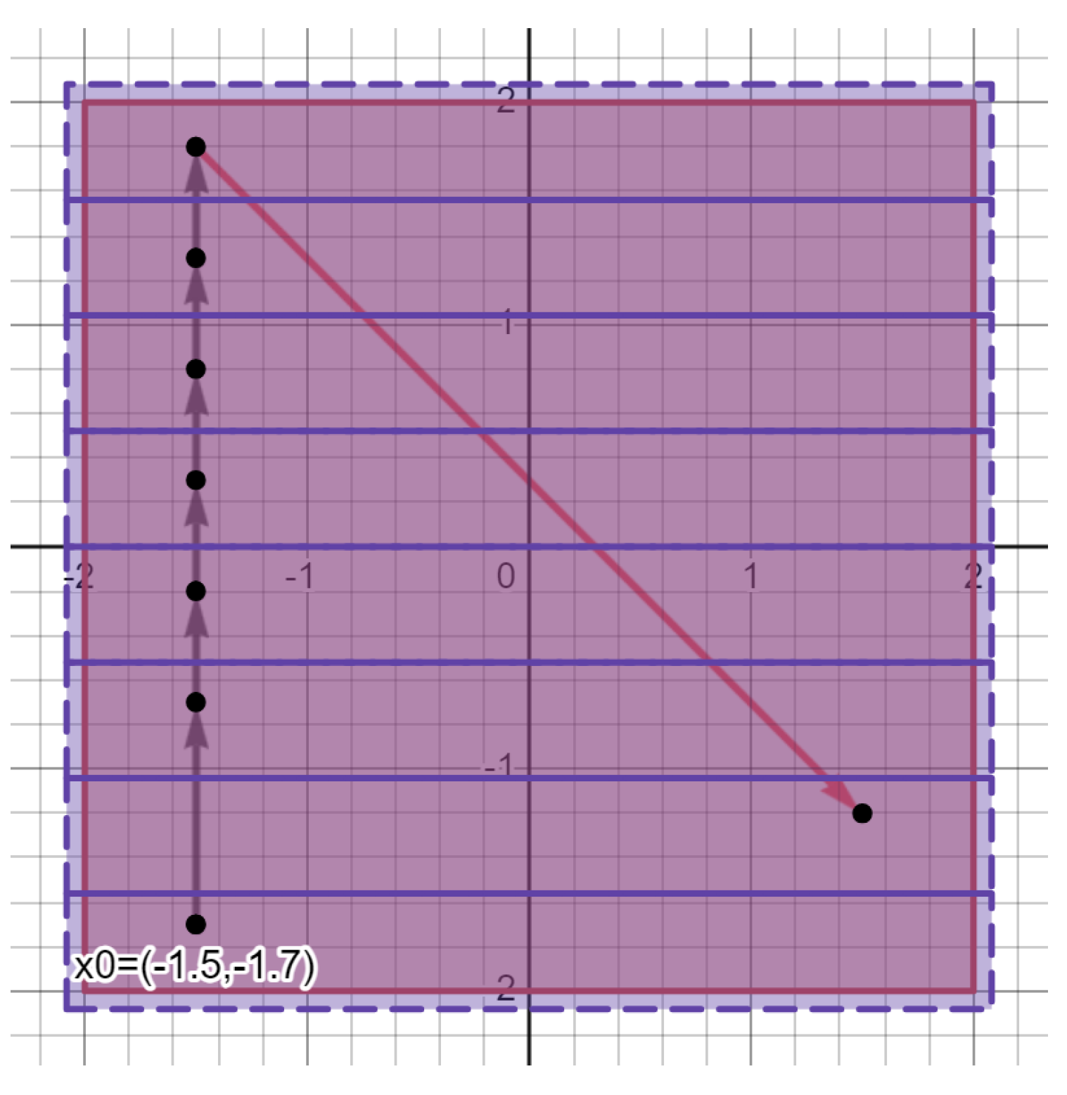
Suppose
- 1.
- 2.
Then one example of , using Section 5.4.1 step 1, (where ) is:
Note, the area of each of the rectangles is , where the borders could be approximated as:
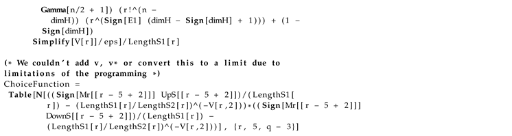
and we’ll illustrate this as purple rectangles covering (i.e., the red square).
Figure 1.
Purple rectangles are the “covers" and the red square is . (Ignore the boundaries)
(Note, the purple rectangles in fig. Figure 1, satisfy step (1) of Section 5.4.1, since the Hausdorff measures in its dimension of the rectangles is and there is a minimum 8 covers over-covering : i.e.,
Definition 3
(Minimum Covers of Measure covering ). We can compute the minimum covers , using the formula:
where )
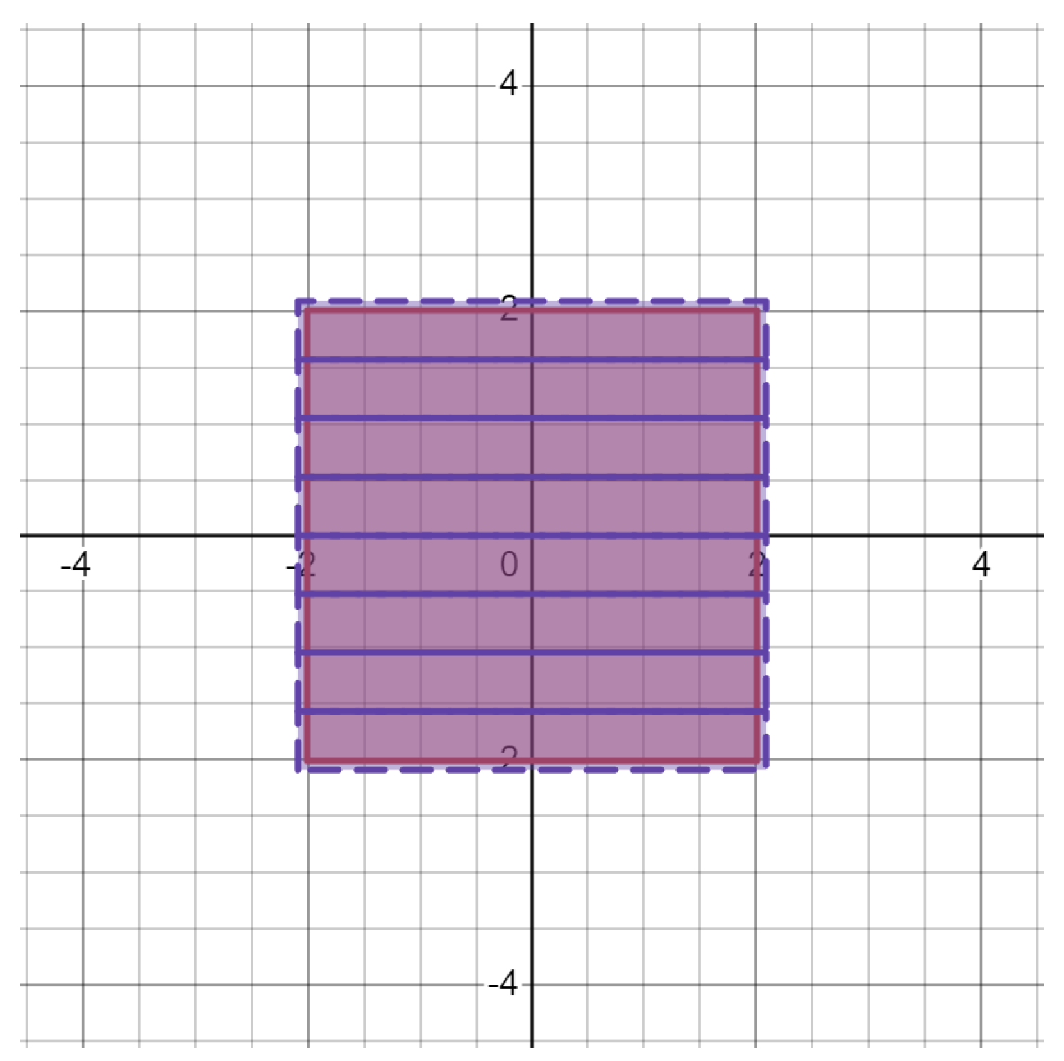
Note the covers in need not be rectangles. In fact, they could be any set as long as the “area" of those sets is , and is over-covered by the smallest number of sets possible. Here is an example:
Figure 2.
The eight purple sets are the “covers" and the red square is . (Ignore the boundaries)
To define this cover, start off with:
Then, for each in , we define:
except where:
such that an example of is:
In the case of , there are uncountably many of different shapes and sizes which we can use. However, these examples were the ones taken.
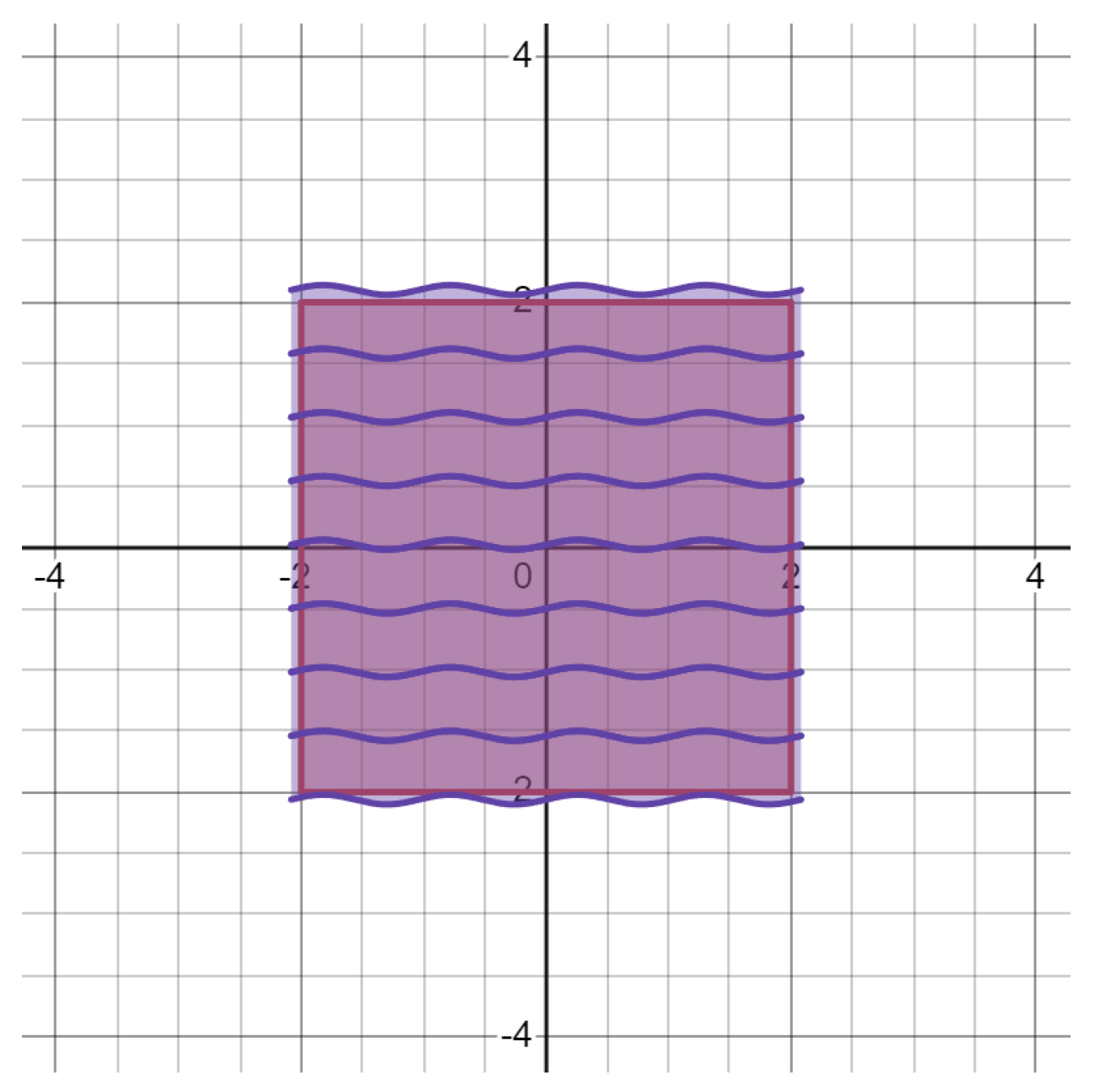
8.2. Example of Section 5.4.1, step 2
Suppose
Then, an example of is:
Below, is an illustration of the sample: i.e., the set of all black points in each purple rectangle of covering :
Figure 3.
The black points are the “sample points", the eight purple rectangles are the “covers", and the red square is . (Ignore the boundaries)
Figure 3.
The black points are the “sample points", the eight purple rectangles are the “covers", and the red square is . (Ignore the boundaries)
Note there are multiple samples we can take, as long as one sample point is taken from each cover in .
8.3. Example of Section 5.4.1, step 3
Suppose
Therefore, consider the following process:
8.3.1. Step 33a
If is:
suppose . Note, the following:
- is the next point in the “pathway" since it’s a point in with the smallest 2-d Euclidean distance to instead of .
- is the third point since it’s a point in with the smallest 2-d Euclidean distance to instead of and .
- is the fourth point since it’s a point in with the smallest 2-d Euclidean distance to instead of , , and .
- we continue this process, where the “pathway" of is:
Notation 9.
If more than one point has the minimum 2-d Euclidean distance from , , , etc. take all potential pathways: e.g., using the sample in Equation (144), if , then since and have the smallest Euclidean distance from , and for point , since and have the smallest Euclidean distance from , we takethreepathways:
8.3.2. Step 33b
Take the length of all line segments in the pathway. In other words, suppose is the n-th dim.Euclidean distance between points . Using the pathway of Equation (145), we want:
Whose distances can be approximated as:
As we can see, the outlier is (i.e., note these outliers become more prominent for ). Therefore, remove from the set of distances:
which we can illustrate with:
Figure 4.
is the start point in the pathway. The black line segments in the “pathway" have lengths which aren’t outliers. The length of the red line segment is an outlier.
Figure 4.
is the start point in the pathway. The black line segments in the “pathway" have lengths which aren’t outliers. The length of the red line segment is an outlier.
8.3.3. Step 33c
To convert the set of distances in Equation (148) into a probability distribution, we take:
Then divide each element in by 3.5
which gives us the probability distribution:
Hence,
8.3.4. Step 33d
Take the shannon entropy of Equation (150):
We shorten to , giving us:
8.3.5. Step 33e
Take the entropy w.r.t all pathways of:
In other words, we’ll compute:
We do this by repeating Section 8.3.1-Section 8.3.4 for different (i.e., in the equations with multiple values, see note 9)
Hence, since the largest value out of Equations (152)–(159) is 2.52164:
References
- a.k.a u/Xixkdjfk, B.K. a.k.a u/Xixkdjfk, B.K. Is there a set with positive Lebesgue measure in any rectangle of the 2-d plane which is extremely non-uniform? https://www.reddit.com/r/mathematics/comments/1eedqbx/comment/lfdf9zb/?context=3.
- Garling, D.J.H. , Inequalities: A Journey into Linear Analysis; Cambridge University Press, 2007; p. 187–205.
- Achour, R.; Li, Z.; Selmi, B.; Wang, T. A multifractal formalism for new general fractal measures. Chaos, Solitons & Fractals 2024, 181, 114655, https://www.sciencedirect.com/science/article/abs/pii/S0960077924002066. [Google Scholar]
- Bedford, T.; Fisher, A.M. Analogues of the Lebesgue density theorem for fractal sets of reals and integers. Proceedings of the London Mathematical Society 1992, 3, 95–124, https://www.ime.usp.br/~afisher/ps/Analogues.pdf.. [Google Scholar]
- Bedford, T.; Fisher, A.M. Ratio geometry, rigidity and the scenery process for hyperbolic Cantor sets. Ergodic Theory and Dynamical Systems 1997, 17, 531–564, https://arxiv.org/pdf/math/9405217. [Google Scholar]
- Krishnan, B. Bharath Krishnan’s ResearchGate Profile. https://www.researchgate.net/profile/Bharath-Krishnan-4.
- John, R. Outlier. https://en.m.wikipedia.org/wiki/Outlier.
- M., G. M., G. Entropy and Information Theory, /: Springer New York: New York [America];, 2011; pp. 61–95., https://ee.stanford.edu/~gray/it.pdf,https://doi.org/https://doi.org/10.1007/978-1-4419-7970-4. [CrossRef]
Disclaimer/Publisher’s Note: The statements, opinions and data contained in all publications are solely those of the individual author(s) and contributor(s) and not of MDPI and/or the editor(s). MDPI and/or the editor(s) disclaim responsibility for any injury to people or property resulting from any ideas, methods, instructions or products referred to in the content. |
© 2025 by the authors. Licensee MDPI, Basel, Switzerland. This article is an open access article distributed under the terms and conditions of the Creative Commons Attribution (CC BY) license (http://creativecommons.org/licenses/by/4.0/).
Copyright: This open access article is published under a Creative Commons CC BY 4.0 license, which permit the free download, distribution, and reuse, provided that the author and preprint are cited in any reuse.


