A Novel Spectral Density Function Validation for Bessel’s Equation in L-N Form

1. Introduction

The concept of spectral density and its role in eigenfunction expansion theory began to emerge in the 19^th and 20^th centuries with developments in Fourier analysis [3]. Besides the seminal work of Joseph Fourier (1768-1830), who introduced the fundamental spectral theory concept of a “Fourier series”, thus enabling the representation of certain types of functions as infinite sums of sinusoids [1], p. 221-222, other prominent mathematicians of the day such as Charles-Francois Sturm (1803-1855) and Joseph Liouville (1809-1882) were some of the earliest pioneers to follow Fourier’s contributions and carry forward the development of spectral theory. Towards the end of the 19^th century and into the early 20^th century, significant contributions towards spectral theory were made by the prominent mathematicians Poincare (1854-1912), Volterra (1860-1940), Hilbert (1862-1943), Fredholm (1866-1927), and Weyl (1885-1955) to name some. The field continued to advance during the 20^th century from important results of E.C. Titchmarsh (1899-1963), John Von Neumann (1903-1957), A. Kolmogorov (1903-1987), and Kunihiko Kodaira (1915-1997), among others (readers may refer to [3,4], or [9] for detailed accounts of these principal contributors to spectral theory as well as many others who were omitted here for the sake of brevity.). Towards the end of the 20^th century and into the 21^st century, contemporary researchers in spectral theory such as Anton Zettl, Barry Simon, Charles Fulton, Fritz Gesztesy, and Maxim Zinchenko, to name some, continued to significantly extend the body of theoretical knowledge, obtaining many new spectral theory results and theorems in their works. Spectral theory remains an active area of mathematical research today and this paper aims to contribute, in small part, to the broad body of results that have already been obtained in the field, particularly, in the area of spectral density functions and their determinations.

2. Background: The Titchmarsh-Weyl m-Function

Consider the general Sturm-Liouville equation:

$$-y^{\prime \prime }(x)+q(x)y(x)=\lambda y(x), x\in (a,\infty ), q(x)\in L_1(a,\infty ),$$

(1)

and $\underset{x\to \infty }{\lim }q(x)=0.$ Suppose x = a is a singular endpoint of the Limit Point (LP) classification as given in [13]. Let {u(x,λ),v(x,λ)} be the fundamental system of (1) normalized so as to have a Wronskian determinant, w_a(u(x,λ),v(x,λ)) = 1, and satisfying the boundary conditions,

$$\left[\begin{array}{cc}u(a,\lambda )& v(a,\lambda )\\ u^{\prime }(a,\lambda )& v^{\prime }(a,\lambda )\end{array}\right]=\left[\begin{array}{cc}1& 0\\ 0& 1\end{array}\right].$$

(2)

The Titchmarsh-Weyl m–function, $m(\lambda ),$ is defined by the requirement

$$\psi (x,y)=u(x,\lambda )+m(\lambda )v(x,y)\in L_2(a,\infty ).$$

(3)

As (1) is a linear differential equation, Ψ(x,y), being a linear combination of solutions to (1) near x = a, satisfies (1) near x = a. Moreover, due to x = a being an LP singular endpoint, Ψ(x,y) and m(λ) are uniquely defined in (3) by this square-integrability requirement given in [11], (p. 86).

The spectral density function f(λ) is then characterized by the Titchmarsh-Kodaira formula,

$$f(\lambda )={\displaystyle \frac{K^{\prime }(\lambda )}{\pi }}=\underset{\epsilon \to 0}{\lim }\left({\displaystyle \frac{-\mathrm{Im}[m(\mu +i\epsilon )]}{\pi }}\right),$$

(4)

where

$$K(\lambda )=\underset{\epsilon \to 0}{\lim }\underset{0}{\overset{\lambda }{\int }}-\mathrm{Im}[m(\mu +i\epsilon )]d\mu .$$

(5)

See [11], p. 43, eq. 3.3.1. In the next section, we define the Appell system.

3. The Appell System

In 1880, M. Appell in [2] gave a companion system to the Sturm-Liouville equation (1) as

$${\displaystyle \frac{dU}{dx}}(x)={\displaystyle \frac{d}{dx}}\left(\begin{array}{l}P(x)\\ Q(x)\\ R(x)\end{array}\right)=\left[\begin{array}{ccc}0& \lambda -q(x)& 0\\ -2& 0& 2(\lambda -q(x))\\ 0& -1& 0\end{array}\right].$$

(6)

Some fundamental properties pertaining to system (6) are now given below (See also [7], p. 6-7).

(i) If y(x) is any solution of the Sturm-Liouville equation (1), then

$U(x)=\left(\begin{array}{c}{(y\prime (x))}^2\\ -2y(x)y\prime (x)\\ y^2(x)\end{array}\right)$ is a solution to the Appell system (6).

(ii) Let {u(x,λ),v(x,λ)} be the fundamental system of (1), where (2) holds. A fundamental system of three linearly independent solutions to (6) is

$$\left\{\left(\begin{array}{c}{(u\prime (x))}^2\\ -2u(x)u\prime (x)\\ u^2(x)\end{array}\right),\left(\begin{array}{l}u\prime (x)v\prime (x)\\ -[u\prime (x)v(x)+u(x)v\prime (x)]\\ u(x)v(x)\end{array}\right),\left(\begin{array}{l}{(v\prime (x))}^2\\ -2v(x)v\prime (x)\\ v^2(x)\end{array}\right)\right\}.$$

(iii) For any solution $U(x)=\left(\begin{array}{l}P(x)\\ Q(x)\\ R(x)\end{array}\right)$to Appell system (6), let the indefinite inner product be defined by: <U₁(x), U₂(x)> = 2(P₁(x)R₂(x) + P₂R₁(x) − Q₁(x)Q₂(x). It follows that:

<U(x), U(x)> = 4P(x)R(x) − Q²(x) = const, ( See [7], pages 6-7).

(iv) Let $U_1(x)=\left(\begin{array}{l}\tilde{P}1(x)\\ \tilde{Q}1(x)\\ \tilde{R}1(x)\end{array}\right)$ and $U_2(x)=\left(\begin{array}{l}{\tilde{P}}_2(x)\\ {\tilde{Q}}_2(x)\\ {\tilde{R}}_2(x)\end{array}\right)$ be any two solutions to Appell system (6) where

$$U_1(x)={\tilde{a}}_1\left(\begin{array}{c}{(u^{\prime }(x))}^2\\ -2u(x)u^{\prime }(x)\\ u^2(x)\end{array}\right)+{\tilde{b}}_1\left(\begin{array}{c}{u}^{\prime }(x)v^{\prime }(x)\\ -[u^{\prime }(x)v(x)+u(x)v^{\prime }(x)]\\ u(x)v(x)\end{array}\right)+{\tilde{c}}_1\left(\begin{array}{c}{(v^{\prime }(x))}^2\\ -2v(x)v^{\prime }(x)\\ v^2(x)\end{array}\right),$$

$$U_2(x)={\tilde{a}}_2\left(\begin{array}{c}{(u^{\prime }(x))}^2\\ -2u(x)u^{\prime }(x)\\ u^2(x)\end{array}\right)+{\tilde{b}}_2\left(\begin{array}{c}{u}^{\prime }(x)v^{\prime }(x)\\ -[u^{\prime }(x)v(x)+u(x)v^{\prime }(x)]\\ u(x)v(x)\end{array}\right)+{\tilde{c}}_2\left(\begin{array}{c}{(v^{\prime }(x))}^2\\ -2v(x)v^{\prime }(x)\\ v^2(x)\end{array}\right).$$

Under these assumptions,

$$\langle U_1(x),U_2(x)\rangle =2({\tilde{a}}_1{\tilde{c}}_2+{\tilde{c}}_1{\tilde{a}}_2)-{\tilde{b}}_1{\tilde{b}}_2\begin{array}{cc} & \mathrm{and}\end{array}\begin{array}{cc} & \langle U_1(x),U_1(x)\rangle \end{array}=4{\tilde{a}}_1{\tilde{c}}_1-{{\tilde{b}}_1}^2.$$

(v) Let y(x) be any solution to the Sturm-Liouville equation (1) and let U(x) = (P(x)Q(x)R(x))^T be a solution to Appell system (6). It follows that:

$${\displaystyle \frac{d}{dx}}[P(x)y^2(x)+Q(x)y(x)y^{\prime }(x)+R(x){(y^{\prime }(x))}^2]=0.$$

(vi) Near x = ∞, x₀ > 0, if either q(x)∈L₁(x₀,∞) or q′(x)∈L₁(x₀,∞), q(x)∈AC_loc(x₀,∞), and $\underset{x\to \infty }{\lim }q(x)=0$, then the terminal value problem below has a unique solution.

$$\{\begin{array}{l}{\displaystyle \frac{dU}{dx}}(x)={\displaystyle \frac{d}{dx}}\left(\begin{array}{c}P(x)\\ Q(x)\\ R(x)\end{array}\right)=\left[\begin{array}{ccc}0& \lambda -q(x)& 0\\ -2& 0& 2(\lambda -q(x))\\ 0& -1& 0\end{array}\right]\left(\begin{array}{c}P(x)\\ Q(x)\\ R(x)\end{array}\right)\hfill \\ \underset{x\to \infty }{\lim }\left(\begin{array}{c}P(x)\\ Q(x)\\ R(x)\end{array}\right)=\left(\begin{array}{c}\sqrt{\lambda }\\ 0\\ 1/\sqrt{\lambda }\end{array}\right), \lambda \in (0,\infty )\hfill \end{array}.$$

(7)

(vii) Let $U_1=\left(\begin{array}{c}{P}_1(x)\\ Q_1(x)\\ R_1(x)\end{array}\right)$be the unique solution to the terminal value problem (7).

It follows that$4\tilde{a}\tilde{c}-{\tilde{b}}^2=4$. Furthermore, when x = 0 is either regular or a RSP of LC/N or LP/N type, x = ∞ is LP/O-N with cut-off ∧ = 0, and q(x) is absolutely integrable near x = ∞ the spectral density function, $f(\lambda ),$ for $\lambda \in (0,\infty ),$ is characterized by:

$$f(\lambda )={\displaystyle \frac{1}{\pi \tilde{a}}}={\displaystyle \frac{1}{\pi [P_1(x)v^2(x,\lambda )+Q_1(x)v(x,y)v^{\prime }(x,y)+R_1(x){(v^{\prime }(x,\lambda ))}^2}},$$

(8)

 where f(λ) is absolutely continuous for $\lambda \in (0,\infty )$ (See [8], p. 40).

The proofs of these properties of the Appell system are well-documented and generally require only algebraic manipulations with no special assumptions on the potential $q(x)$according to Fulton in [7], p. 6. For this reason, the proofs of the properties (i)-(vii) are omitted in this paper. In the next section, we’ll utilize these properties and demonstrate the viability of the spectral density function characterization given in (vii) by providing the first nontrivial example of a spectral density function calculation by use of (8), as applied to the Bessel equation in L-N form.

4. Calculation of the SDF for Bessel’s Equation in Liouville-Normal Form

Consider the Bessel Equation in L-N form

$$-y^{\prime \prime }(x)+\left({\displaystyle \frac{{\nu }^2-1/4}{x^2}}\right)y(x)=\lambda y(x),$$

(9)

for a < x < ∞, a > 0 and with v ≠ 0, 1, 2, … Here observe that x = ∞ is a LP/O-N singular endpoint with cutoff λ = 0. Let {u(x,λ), v(x,λ)} be the fundamental system to (9) such that $\left[\begin{array}{cc}u(a,\lambda )& v(a,\lambda )\\ u^{\prime }(a,\lambda )& v^{\prime }(a,\lambda )\end{array}\right]=\left[\begin{array}{cc}1& 0\\ 0& 1\end{array}\right]$, for all $\lambda \in (0,\infty )$. Here the potential function $q(x)={\displaystyle \frac{v^2-\raisebox{1ex}{$1$}\!\left/ \!\raisebox{-1ex}{$4$}\right.}{x^2}}\in L_1(a,\infty )$ and thus the Appell system property (vi), from above, holds. The corresponding Appell system terminal value problem for (9) is then

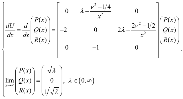(10)

Let U₁(x) be the unique solution to (10) where $\tilde{a}$, $\tilde{b}$, and $\tilde{c}$ are defined by the relation

$$U_1(x)={\tilde{a}}_1\left(\begin{array}{c}{(u^{\prime }(x))}^2\\ -2u(x)u^{\prime }(x)\\ u^2(x)\end{array}\right)+{\tilde{b}}_1\left(\begin{array}{c}{u}^{\prime }(x)v^{\prime }(x)\\ -[u^{\prime }(x)v(x)+u(x)v^{\prime }(x)]\\ u(x)v(x)\end{array}\right)+{\tilde{c}}_1\left(\begin{array}{c}{(v^{\prime }(x))}^2\\ -2v(x)v^{\prime }(x)\\ v^2(x)\end{array}\right).$$

(11)

The fundamental system to ODE (9), {u(x,y), v(x,λ)}, which satisfies the Wronskian requirement, w_a(u(x,λ), v(x, λ)) = 1, is uniquely determined with

$$v(x,y)=C_1\cdot \sqrt{x}{J}_v(\sqrt{\lambda }x)+C_2\cdot \sqrt{x}{Y}_v(\sqrt{\lambda }x),$$

(12)

$$u(x,y)=C_3\cdot \sqrt{x}{J}_v(\sqrt{\lambda }x)+C_4\cdot \sqrt{x}{Y}_v(\sqrt{\lambda }x),$$

(13)

where the constants C₁, C₂, C₃, and C₄ are given by

$$C_1={\displaystyle \frac{-\pi \sqrt{a}}{2}}{Y}_v(a\sqrt{\lambda }),\begin{array}{cc} & C_2=\end{array}{\displaystyle \frac{\pi \sqrt{a}}{2}}{J}_v(a\sqrt{\lambda }),$$

(14)

$$C_3={\displaystyle \frac{\pi }{4\sqrt{a}}}{Y}_v(a\sqrt{\lambda })+{\displaystyle \frac{\pi }{2}}\sqrt{a\cdot \lambda }\cdot Y_v^{\prime }(a\sqrt{\lambda }),\begin{array}{cc} & \mathrm{and}\end{array}\begin{array}{cc} & C_4=\end{array}{\displaystyle \frac{-\pi }{4\sqrt{a}}}{J}_v(a\sqrt{\lambda })-{\displaystyle \frac{\pi }{2}}\sqrt{a\cdot \lambda }\cdot J_v^{\prime }\sqrt{\lambda }.$$

The definitions for these suitably normalized solutions, u(x,y), v(x,λ), along with the indicated values for C₁, C₂, C₃, and C₄ in (14), ensure that the Wronskian determinant, w_a(u(x,y), v(x,λ)) = 1, as required. The pertinent Wronskian relations for the Bessel functions  and  can be found in [12], p. 76. Now that the fundamental system to (9) has been given explicitly, we can use the characterization of solution as given in (11) and impose the terminal condition in (10) to yield

$$\{\begin{array}{l}\sqrt{\lambda }=\underset{x\to \infty }{\lim }\{\tilde{a}{(u^{\prime }(x,y))}^2+\tilde{b}{u}^{\prime }(x,y)v^{\prime }(x,y)+\tilde{c}{(v^{\prime }(x,\lambda ))}^2\}\hfill \\ 0=\underset{x\to \infty }{\lim }\{\tilde{a}(-2u(x,y)u^{\prime }(x,y)+\tilde{b}[(-1)(u^{\prime }(x,y)v(x,y)+u(x,y)v^{\prime }(x,y)]+\tilde{c}(-2v(x,\lambda )v^{\prime }(x,y))\},\hfill \\ 1/\sqrt{\lambda }=\underset{x\to \infty }{\lim }\{\tilde{a}{u}^2(x,y)+\tilde{b}u(x,\lambda )v(x,\lambda )+\tilde{c}{v}^2(x,\lambda )\hfill \end{array}$$

(15)

where $\tilde{a}$, $\tilde{b}$, and $\tilde{c}$ are uniquely defined by (15) as guaranteed by Appell system property (vi). Now for further progress towards obtaining explicit representations of $\tilde{a}$, $\tilde{b}$, $\tilde{c}$ and then f(λ) as characterized by (8), we next make use of well-known asymptotic relations for the Bessel functions J_v(x) and Y_v(x) as x → ∞. The asymptotic relations for the Bessel functions near infinity, given below as (16)-(19), are in many books (See for instance the extensive work of G.N. Watson, A Treatise on the Theory of Bessel Functions, [12], p. 199). As x → ∞,

$$x^{{\displaystyle \raisebox{1ex}{$1$}\!\left/ \!\raisebox{-1ex}{$2$}\right.}}{J}_v(\sqrt{\lambda }\cdot x)=\sqrt{{\displaystyle \frac{2}{\pi \cdot \sqrt{\lambda }}}}\cos (\sqrt{\lambda }\cdot x-{\displaystyle \frac{\lambda v}{2}}-{\displaystyle \frac{\pi }{4}})+O({\displaystyle \frac{1}{x}}),$$

(16)

$$x^{{\displaystyle \raisebox{1ex}{$1$}\!\left/ \!\raisebox{-1ex}{$2$}\right.}}{Y}_v(\sqrt{\lambda }\cdot x)=\sqrt{{\displaystyle \frac{2}{\pi \cdot \sqrt{\lambda }}}}\sin (\sqrt{\lambda }\cdot x-{\displaystyle \frac{\pi v}{2}}-{\displaystyle \frac{\pi }{4}})+O({\displaystyle \frac{1}{x}}),$$

(17)

$${\left(x^{{\displaystyle \raisebox{1ex}{$1$}\!\left/ \!\raisebox{-1ex}{$2$}\right.}}{J}_v(\sqrt{\lambda }\cdot x)\right)}^{\prime }=\sqrt{{\displaystyle \frac{2}{\pi \cdot \sqrt{\lambda }}}}[-\sqrt{\lambda }\sin (\sqrt{\lambda }\cdot x-{\displaystyle \frac{\pi v}{2}}-{\displaystyle \frac{\pi }{4}})+O({\displaystyle \frac{1}{x}})],$$

(18)

$${\left(x^{{\displaystyle \raisebox{1ex}{$1$}\!\left/ \!\raisebox{-1ex}{$2$}\right.}}{Y}_v(\sqrt{\lambda }\cdot x)\right)}^{\prime }=\sqrt{{\displaystyle \frac{2}{\pi \cdot \sqrt{\lambda }}}}[\sqrt{\lambda }\cos (\sqrt{\lambda }\cdot x-{\displaystyle \frac{\pi v}{2}}-{\displaystyle \frac{\pi }{4}})+O({\displaystyle \frac{1}{x}})].$$

(19)

By letting $w(x,\lambda )=w(x):=\sqrt{\lambda }x-{\displaystyle \frac{\nu \pi }{2}}-{\displaystyle \frac{\pi }{4}}$ and applying (16)-(19) to (15), we obtain

$$\sqrt{\lambda }=\underset{x\to \infty }{\lim }\left({\displaystyle \frac{2\sqrt{\lambda }}{\pi }}\right)\cdot \left\{\begin{array}{l}{\sin }^2(w(x))\cdot [\tilde{a}{(C_3)}^2+\tilde{b}{C}_1{C}_3+\tilde{c}{(C_1)}^2]\hfill \\ +{\cos }^2(w(x))\cdot [\tilde{a}{(C_4)}^2+\tilde{b}{C}_2{C}_4+\tilde{c}{(C_2)}^2]\hfill \\ +\sin (w(x))\cos (w(x))\cdot [-2\tilde{a}{C}_3{C}_4-\tilde{b}(C_2{C}_3-C_1{C}_4)-2\tilde{c}{C}_1{C}_2]\hfill \end{array}\right\}=o\left({\displaystyle \frac{1}{x}}\right),$$

(20)

$$0=\underset{x\to \infty }{\lim }\left({\displaystyle \frac{2}{\pi }}\right)\cdot \left\{\begin{array}{l}{\sin }^2(w(x))\cdot [-2\tilde{a}{C}_3{C}_4-\tilde{b}(C_2{C}_3+C_1{C}_4)-2\tilde{c}{C}_1{C}_2]\hfill \\ +{\cos }^2(w(x))\cdot {[2\tilde{a}{C}_3{C}_4)}^2+\tilde{b}(C_2{C}_3+C_1{C}_4)+2\tilde{c}{C}_1{C}_2]\hfill \\ +\sin (w(x))\cos (w(x))\cdot [2\tilde{a}({(C_4)}^2-{(C_3)}^2)+2\tilde{b}(C_2{C}_4-C_1{C}_3)+2\tilde{c}({(C_1)}^2-{(C_1)}^2)]\hfill \end{array}\right\}=o\left({\displaystyle \frac{1}{x}}\right)$$

(21)

and

$${\displaystyle \frac{1}{\sqrt{\lambda }}}=\underset{x\to \infty }{\lim }\left({\displaystyle \frac{2}{\pi \sqrt{\lambda }}}\right)\cdot \left\{\begin{array}{l}{\sin }^2(w(x))\cdot [\tilde{a}{(C_4)}^2+\tilde{b}{C}_2{C}_4+\tilde{c}{(C_2)}^2]\hfill \\ +{\cos }^2(w(x))\cdot [\tilde{a}{(C_3)}^2+\tilde{b}{C}_1{C}_3+\tilde{c}{(C_1)}^2]\hfill \\ +\sin (w(x))\cos (w(x))\cdot [2\tilde{a}{C}_3{C}_4+\tilde{b}(C_2{C}_3+C_1{C}_4)+2\tilde{c}{C}_1{C}_2]\hfill \end{array}\right\}=o\left({\displaystyle \frac{1}{x}}\right).$$

(22)

Now to satisfy relations (20)-(22), nine equations emerge, three of which are independent,

$$\{\begin{array}{l}\tilde{a}{(C_3)}^2+\tilde{b}{C}_1{C}_3+\tilde{c}{(C_1)}^2={\displaystyle \frac{\pi }{2}}\hfill \\ \tilde{a}{(C_4)}^2+\tilde{b}{C}_2{C}_4+\tilde{c}{(C_2)}^2={\displaystyle \frac{\pi }{2}}\hfill \\ 2\tilde{a}{C}_3{C}_4+\tilde{b}(C_1{C}_4+C_2{C}_3)+2\tilde{c}{C}_1{C}_2=0\hfill \end{array},$$

(23)

or in a matrix form

$$\left[\begin{array}{ccc}{(C_3)}^2& C_1{C}_3& {(C_1)}^2\\ {(C_4)}^2& C_2{C}_4& {(C_2)}^2\\ 2C_3{C}_4& (C_1{C}_4+C_2{C}_3)& 2C_1{C}_2\end{array}\right]\left(\begin{array}{c}\tilde{a}\\ \tilde{b}\\ \tilde{c}\end{array}\right)=\left(\begin{array}{c}{\displaystyle \raisebox{1ex}{$\pi $}\!\left/ \!\raisebox{-1ex}{$2$}\right.}\\ {\displaystyle \raisebox{1ex}{$\pi $}\!\left/ \!\raisebox{-1ex}{$2$}\right.}\\ 0\end{array}\right)$$

(24)

The solution to (24) is computed via Mathematica to be

$$\tilde{a}={\displaystyle \frac{\pi ({(C_1)}^2+{(C_1)}^2)}{2{(C_2{C}_3-C_1{C}_4)}^2}},\tilde{b}={\displaystyle \frac{-\pi (C_1{C}_3+C_2{C}_4)}{{(C_2{C}_3-C_1{C}_4)}^2}},\begin{array}{cc} & \mathrm{and}\end{array}\begin{array}{cc} & \tilde{c}={\displaystyle \frac{\pi ({(C_3)}^2+{(C_4)}^2)}{2{(C_2{C}_3-C_1{C}_4)}^2}}\end{array}.$$

(25)

Inserting the definitions for C₁, C₂, C₃, and, C₄ as defined in (14) now reveals that

$$\tilde{a}={\displaystyle \frac{a\pi }{2}}({J^2}_v(a\sqrt{\lambda })+{Y^2}_v(a\sqrt{\lambda })),$$

(26)

$$\tilde{b}={\displaystyle \frac{\pi }{2}}({J^2}_v(a\sqrt{\lambda })+{Y^2}_v(a\sqrt{\lambda }))+\pi \cdot a\sqrt{\lambda }(J_v(a\sqrt{\lambda })\cdot J_v^{\prime }a\sqrt{\lambda })+Y_v(a\sqrt{\lambda })\cdot Y_v^{\prime }a\sqrt{\lambda }),$$

(27)

$$\begin{array}{c}\tilde{c}={\displaystyle \frac{\pi }{8a}}\left({J^2}_v(a\sqrt{\lambda })+{Y^2}_v(a\sqrt{\lambda })\right)+{\displaystyle \frac{a\pi \lambda }{2}}\left({\left((J_v^{\prime }(a\sqrt{\lambda })\right)}^2+{\left(Y_v^{\prime }(a\sqrt{\lambda })\right)}^2\right)\\ +{\displaystyle \frac{\pi \sqrt{\lambda }}{2}}\left(J_v(a\sqrt{\lambda })\cdot J_v^{\prime }(a\sqrt{\lambda })+Y_v(a\sqrt{\lambda })\cdot Y_v^{\prime }(a\sqrt{\lambda })\right)\end{array}.$$

(28)

Finally, we apply the characterization of the spectral density function given in (8), obtaining

$$f(\lambda )={\displaystyle \frac{2}{a{\pi }^2}}\left({\displaystyle \frac{1}{{J^2}_v(a\sqrt{\lambda })+{Y^2}_v(a\sqrt{\lambda })}}\right).$$

(29)

This work, culminating in equation (29), constitutes an original determination of the spectral density function for Bessel’s Equation in L-N form, obtained using the new method proposed by Fulton, Pearson, and Pruess in [7]. In the next brief section, we’ll validate this result obtained using independent checks.

5. Validation of Results

(A) To confirm the validity of the representations obtained above for $\tilde{a}$ and f(λ), eq.’s (26) and (29), we compare the spectral density function obtained in (29) with the classical spectral density function result for the Bessel Equation (6), obtained by E.C. Titchmarsh via the Titchmarsh-Kodaira formula (4) (See [11], p. 86). Here we find full agreement in the f(λ) representations and so the f(λ) in equation (29) is validated. As f(λ), given in equation (29), is computed directly by use of $\tilde{a}$ in (26) (which was obtained by solving the Appell system terminal value problem (10)), we may conclude that the representation in (26) for $\tilde{a}$ is validated.

(B) To validate the representation of $\tilde{b}$, in eq. (27), the theory of C. Fulton, D. Pearson, and S. Pruess in [7], eq. 4.22 is employed, whereby the Titchmarsh-Weyl m-function has the form,

$$m(\lambda )=-{\displaystyle \frac{\tilde{b}}{2\tilde{a}}}+i{\displaystyle \frac{1}{\tilde{a}}},$$

(30)

According to classical theory of Titchmarsh in [11], the m-function for Bessel Equation (9) is

$$m(\lambda )=-\sqrt{a}\left({\displaystyle \frac{J_v^{\prime }(a\sqrt{\lambda })+i{Y}_v^{\prime }(a\sqrt{\lambda })}{J_v(a\sqrt{\lambda })+i{Y}_v(a\sqrt{\lambda })}}\right)-{\displaystyle \frac{1}{2a}}.$$

(31)

By calculation of m(λ) via (30) using (16)-(19), (26), and (27), after minor algebraic manipulations, we indeed obtain the classical m-function result given in (31) and thus we may conclude that the calculation of $\tilde{b}$, as was determined in (27), is validated.

(C) To validate the representation of $\tilde{c}$obtained in (28), according to the Appell system theory in property (vii), necessarily $4\tilde{a}\tilde{c}-{\tilde{b}}^2=4$. While this calculation to validate $\tilde{c}$ is rather tedious, we will give some details of it here to conclude our investigation. Inserting the values for $\tilde{a}$, $\tilde{b}$, and $\tilde{c}$, as given in (26)-(28), into the equation $4\tilde{a}\tilde{c}-{\tilde{b}}^2=4$, and expansion yields twenty-eight terms on the LHS, all of which are products of the Bessel functions $J_{\nu }$, $Y_{\nu }$, and their derivatives, and all of which are having the argument $a\sqrt{\lambda }$. Multiple pairs of these terms (and sometimes triples) combine, are opposites, and cancel leaving just three terms that do not immediately cancel by trivial algebraic manipulation. At this stage, the LHS of $4\tilde{a}\tilde{c}-{\tilde{b}}^2=4$ takes the form

$$4\tilde{a}\tilde{c}-{\tilde{b}}^2=(a^2{\pi }^2\lambda )(J_{\nu }^2{Y^{\prime }}_{\nu }^2+{J^{\prime }}_{\nu }^2{Y}_{\nu }^2-2J_{\nu }{J^{\prime }}_v{Y}_{\nu }{Y^{\prime }}_{\nu }),$$

(32)

with the arguments of these Bessel functions all being $a\sqrt{\lambda }$. To make further progress, we find that the RHS of (32) factors giving

$$4\tilde{a}\tilde{c}-{\tilde{b}}^2=(a^2{\pi }^2\lambda ){(J_{\nu }{Y^{\prime }}_{\nu }-{J^{\prime }}_{\nu }{Y}_{\nu })}^2.$$

(33)

Finally, to obtain the value of 4 on the RHS of (33), we employ a Wronskian identity from Watson’s [12], p. 76, with his z-argument replaced by $a\sqrt{\lambda }$. This identity takes the form of

$$J_v(a\sqrt{\lambda })\cdot {Y^{\prime }}_{\nu }(a\sqrt{\lambda })-{J^{\prime }}_{\nu }(a\sqrt{\lambda })\cdot Y_{\nu }(a\sqrt{\lambda })={\displaystyle \frac{2}{\pi a\sqrt{\lambda }}}.$$

(34)

Upon insertion of (34) into (33), we complete our validation of $\tilde{c}$.

6. Conclusions

In this paper, an original calculation of a spectral density function was performed using the new method of C. Fulton, D. Pearson, and S. Pruess [7]. Prior to this work, no other nontrivial example of such a calculation using the characterization of f(λ) given in (8) had been demonstrated. Future authors may follow the prescribed outline given above to calculate additional spectral density functions for Sturm-Liouville equations of the form (1)-(2).

References

- Agarwal, Ravi P., Sen, Syamal K., (2014). Creators of Mathematical and Computational Sciences, Springer.
- Appell, M., (1880). Sur la transformation des équations différentielles linéaires, In Comptes Rendus Acad. Sci. Paris, Semestre 19, p. 211-214.
- Davies, E.B., (1995). Spectral Theory and Differential Operators, Cambridge Uni. Press.
- Dunford, N and Schwartz, J. (1958) Linear Operators Parts I-III, Interscience Publishers.
- Fulton, C., Pearson, D., and Pruess, S., (2005). Computing the spectral function for singular Sturm–Liouville problems, J. Comput. Appl. Math. 176 p. 131–162. [CrossRef]
- Fulton, C., Pearson, D., and Pruess, S., (2008). New characterizations of spectral density functions for singular Sturm–Liouville problems, Journal of Computational and Applied Mathematics, 212, p. 122-213. [CrossRef]
- Fulton, C., Pearson, D., and Pruess, S., (2014). Estimating spectral density functions for Sturm–Liouville problems with two singular endpoints, IMA Journal of Numerical Analysis, 34, p. 609-650. [CrossRef]
- Fulton, C., (2015). The Connection Problem for Solutions of Sturm-Liouville Problems with two singular endpoints, and its relation to m-functions, in Olberwolfach Report 1/2015, Report on Olberwolfach Workshop on Spectral Theory and Weyl Functions, January 4-10, 2015, Olberwolfach, Germany. [CrossRef]
- Steen, L.A. (1973), Highlights in the history of spectral theory, Amer. Math. Monthly, 80, p. 359-381. [CrossRef]
- Titchmarsh, E.C., (1932). The Theory of Functions, Oxford University Press.
- Titchmarsh, E.C., (1962). Eigenfunction expansions associated with second-order differential equations, 2nd ed., Clarenden Press, Oxford (1st Ed 1946).
- Watson, G.N., (1944). A Treatise on the Theory of Bessel Functions 2nd Edition, Cambridge University Press, (1st Ed. 1922; 2nd Ed. 1944).
- Weyl, H., (1910). Über gewöhnliche Differentialgleichungen mit Singularitäten und die zugehörigen Entwicklungen willkürlicher Funktionen, Math. Ann. 68.
Disclaimer/Publisher’s Note: The statements, opinions and data contained in all publications are solely those of the individual author(s) and contributor(s) and not of MDPI and/or the editor(s). MDPI and/or the editor(s) disclaim responsibility for any injury to people or property resulting from any ideas, methods, instructions or products referred to in the content. |
© 2024 by the authors. Licensee MDPI, Basel, Switzerland. This article is an open access article distributed under the terms and conditions of the Creative Commons Attribution (CC BY) license (http://creativecommons.org/licenses/by/4.0/).
Copyright: This open access article is published under a Creative Commons CC BY 4.0 license, which permit the free download, distribution, and reuse, provided that the author and preprint are cited in any reuse.