

Submitted:
20 August 2024
Posted:
20 August 2024
You are already at the latest version
Abstract
This study proposed a regression model for predicting fatigue properties based on crucial weld geometry factors in lap-welded joints with gaps using statistical analysis. Welding conditions were varied to build various weld geometries in joints configured in a lap from with gaps of 0, 0.2, 0.5, and 1.0 mm, and 87 S-N curves for the lap-welded joints were derived. As input variables, 17 weld geometry factors (7 lengths, 7 angles, and 3 area factors) were selected. The slope of the S-N curve using Basquin model from the S-N curve and the safe fatigue strength were selected as output variables for prediction to develop the regression model. Multiple linear regression models, multiple non-linear regression models, and second-order polynomial regression models were proposed to predict fatigue properties. Backward elimination was applied to simplify the models and reduce overfitting. Among the three proposed regression models, the multiple non-linear regression model had a coefficient of determination greater than 0.86. In lap-welded joints with gaps, the weld geometry factors representing fatigue properties were identified through standardized regression coefficients, and four weld geometry factors related to stress concentration were proposed.
Keywords:
Lap welded joint
; GMAW
; fatigue characteristic prediction
; regression model
; joint gap
; weld geometry
1. Introduction
The automobile chassis collectively refers to all the parts of a car, excluding the body, consisting of the frame, powertrain, suspension, steering, and braking components. Among these, the frame serves as the fundamental skeleton of the chassis, comprising cross-members, lower arms, and coupled torsion beam axle, and it is located at the very bottom of the car, requiring durability against repetitive loads during operation.
The chassis frame, which requires fatigue durability, mainly comprises lap joints and is primarily manufactured using GMAW to ensure strength. In GMAW, using filler wire, the weld metal will impart a geometric shape to the joint is inevitable. This acts as a stress concentration point due to repeated fatigue, leading to fracture initiation and ultimately decreasing the component’s fatigue durability. Even when high-strength steel is applied to chassis components for weight reduction, the benefits of high-strength steel are lost due to the notch effect of lap welds [1,2]. In welded joints with geometric shapes, such as lap welds, the bead shape has a more significant impact on fatigue characteristics than the weld’s microstructure [3,4]. Previous studies have reported that, particularly in lap joints, improving the weld toe angle alleviates stress concentration at the notch area of the weld, thereby enhancing fatigue characteristics [5,6,7,8,9]. Prior investigations examining the fatigue characteristics of lap joints have compared the relationship between weld toe angle and fatigue characteristics only in flawless joints without gaps or with a consistent gap.
Differences in the amount of spring-back due to the non-uniformity of alloying elements even within the same material, cutting errors, and machining dimensional tolerances make it impossible to completely eliminate or maintain a consistent joint gap in welded parts. The presence of gaps in the joint can lead to welding defects, even when welding is performed under the same conditions on identical components [10]. It has been reported that gaps deteriorate fatigue properties [11,12]. Kim et at [13] reported in the weld of lap joints, an increase in the joint gap caused the filler metal of the GMAW process to fill the gap, resulting in a smoother weld profile and an increase in the apparent weld toe angle. However, they confirmed that stress concentration at the weld root occurred, leading to decreased fatigue strength. Therefore, they suggested considering geometric shapes other than the weld toe angle for lap welds with gaps requiring fatigue characteristics.
Deriving S-N curves to determine fatigue characteristics is a time-consuming and expensive process. Therefore, methods and research for predicting fatigue characteristics are being actively pursued. Traditionally, after Palmgren introduced the concept of damage accumulation [14] and Miner introduced the linear damage rule [15], many damage and prediction models have been developed. Fatemi et al [16] and Hectors et al [17] reviewed the article paper on cumulative damage and life prediction models for fatigue. They have confirmed that linear and non-linear fatigue cumulative damage rules can predict fatigue characteristics based on fatigue life calculations. These calculations reflect the material and weld joint properties and the stress-strain relationship resulting from repetitive loading cycles. Machine learning methods have recently been applied to process data, including noisy data, and learn complex non-linear relationships to predict the fatigue characteristics of materials and weldments based on data without prior assumptions. Various machine learning algorithms, including artificial neural networks, convolutional neural networks, residual neural networks, and gradient boosting decision trees, have been applied to predict the fatigue characteristics of materials and weldments, demonstrating excellent fatigue prediction performance [18,19,20,21].
In predicting the fatigue characteristics of the lap weld, which is the most commonly used single-sided joint in chassis components, it is considered difficult to apply a fatigue cumulative damage model for load cycles due to the challenge of reflecting the weld shape (non-uniform stress distribution) that changes due to welding conditions and disturbances during welding. Machine learning-based prediction models operate as black-box surrogate models between input and output parameters, making the internal decision-making process opaque and difficult to interpret. Additionally, it is challenging to assign physical meaning to the input variables in relation to the output variables [22]. Although studies to fatigue characteristics are being reported for chassis components requiring fatigue properties, research on predicting fatigue characteristics remains relatively scarce. The lack of research on predicting the fatigue characteristics of automotive chassis components is due to the widely accepted fact that improving the weld toe angle of typical lap joints enhances fatigue characteristics. However, the need for additional research on predicting the fatigue characteristics of lap welds, especially considering the gap, is urgent. This is particularly crucial in actual components where it is impossible to eliminate or maintain a consistent joint gap.
This study not only identified the significant weld geometry factors affecting fatigue characteristics in lap welds with gaps but also predicted an S-N curve based on a regression model. Lap welding was performed on GA 590 MPa 2.3 mm, which is widely used in chassis components. The joint gap size (Gap), welding process (WP), wire feed rate (WFR), and welding speed (WS) were varied to achieve different weld geometric shapes. A total of 87 S-N curves were derived through fatigue tests on lap joint specimens with various weld shapes. Through cross-sectional analysis, 17 weld geometry measurements (seven length factors, seven angle factors, and three area factors) were used as input variables. Three regression models were proposed to predict the slope of the S-N curve and the fatigue strength (fatigue strength at 2 × 10⁶ cycles) with a safety factor. Three models were developed using backward elimination: a multiple linear regression model, a multiple non-linear regression model, and a second-order polynomial regression model. The significant factors affecting fatigue characteristics were proposed through standardized regression coefficients.
2. Experimental Procedure
2.1. Welding Procedure
A GA 590 MPa grade steel sheet of thickness 2.3 mm was considered for the welding experiment, and AWS A5.18 ER70S-3 of diameter 1.2 mm was used as the filler wire. Table 1 shows the chemical composition and mechanical properties of the base material and filler wire.
The base material was cut to a size of 150 × 300 mm, and the direction of joint was selected in two forms, shown in Figure 1. Various weld joint configurations were considered to predict fatigue characteristics through weld joint shapes, and welding was conducted using diverse welding processes and conditions. In order to confirm fatigue characteristics based on joint gap, four gap conditions were selected: 0 mm, 0.2 mm, 0.5 mm, and 1.0 mm. Cold metal transfer (CMT, Fronius co.) and direct current (DC, Daihen co.) were applied to the two types of joints prepared for the WP. WFR was varied in three levels, which included 5.0 – 9.0 m/min during CMT and 3.0 – 7.0 m/min during DC application. Two levels of WS were selected as 60 and 80 cm/min. Additionally, contact tip to work distance (CTWD, α) and work angle were fixed at 15 mm and 45°, respectively. A 90 % Ar + 10 % CO2 mixed shielding gas was provided at a flow rate of 25 L/min. The welding experiment was repeated five times under the same conditions to produce a fatigue specimen. The detailed welding conditions are listed in Table 2.
2.2. Fatigue Test Procedure
The fatigue test specimens were manufactured by referring to the ASTM E466 standard for welding specimens (Figure 2) [23]. A spacer was inserted by combining the thickness of the gap and base material. Radiography inspection was performed on fabricated test specimens, and fatigue tests were conducted on the test specimens without defects such as porosity. We employed fatigue testing equipment (Instron 8801, Instron Co.) with a maximum load of 100 kN. Table 3 and Figure 3 show the fatigue test conditions and a schematic of the applied fatigue stress amplitude variations. The stress ratio of a specific component of an automobile chassis was adopted, and the fatigue limit was set at the commonly used 2 × 10⁶ cycles. A total of 87 S-N curves are derived through fatigue testing and used as data to predict fatigue characteristics. In this study, the fatigue test specimens were denoted in the order of weld joint – WP – WFR – WS – Gap. For example, under the conditions A position, WP CMT, WFR 7.0 m/min, WS 60 cm/min, Gap 0.2 mm (Table 2), it is expressed as A–C (CMT: C, DC: D)–7.0–60–0.2.
3. Method for Developing the S-N Curve Prediction Model
3.1. Selection of Independent and Dependent Variables
The weld joint geometry data extracted and used as independent variables. A lap-joint weld typically appears in a shape similar to that illustrated in Figure 4, As criteria for configuration of weld shape to be used in a fatigue prediction model, 17 parameters were extracted. The method for extracting the 17 parameters is summarized in Figure 4. In the geometry of the lap weld joint, seven factors related to length including leg length and penetration depth [24,25,26,27], seven factors related to angle [28], such as toe angle, and three factors about have been derived [28].
3.2. Selection of Dependent Variables
The response variable for developing the S-N curve prediction model was constructed using the fatigue dataset. For each S-N curve, a logarithm was considered at the stress range (, and the (Eq. 1) was applied the determine and [29].
where is the material property, is the fatigue life as the number of cycles to failure under a constant load, and is the .
In the S-N curve for the weld joint, establishing a safety factor to prevent fatigue failure is essential. and were determined by applying M-2SD in Eq. 2 [30].
where represents fatigue life at , while signifies the mean life at Essentially, M-2SD represents fatigue life re-expressed by subtracting twice the standard deviation from the average fatigue life at . This value was used to design a safety factor in the S-N curve using the . incorporating the safety factor was used as the dependent variable to predict fatigue characteristics through weld joint geometry parameters. Only was predicted, while was not predicted. The reasons are explained in next section. Predicting the endurance fatigue limit (2 × 10⁶ cycles) on the S-N curve was essential. Fatigue strength at a fatigue life of 2 × 10⁶ cycles was derived from the using M-2SD and compared with the fatigue strength obtained through fatigue testing. Lower fatigue strength was defined as safety fatigue strength , considering stability against fatigue failure. The schematic for is presented in Figure 5. The critical factors obtained from and , along with the individually applied value of stress levels, included independent variables that were used to predict the overall fatigue life.
.
3.3. Development of an S-N Curve Prediction Model through Statistical Analysis
We employed a statistical analysis method, a regression model approach, to predict the S-N curve. A regression model is a statistical analysis technique used to predict the value of dependent variables from independent variables by assuming a mathematical model between them. A generalized linear regression model was constructed, as given in Eq. 3.
where denotes a scalar function with independent variables as arguments and includes non-linear and polynomial expressions. In this study, multiple linear, non-linear, and second-order polynomial regression models were derived using the backward elimination method.
4. Result of Fatigue Behavior
A total of 87 S-N curve were derived from varying welding conditions. Figure 6 illustrates some of them selectively presented. It was observed that as WFR increase, fatigue strength and life at a constant load increase (Figure 6 (a)). Conversely, an increase in WS resulted in decreased fatigue life and strength (Figure 6 (b)). As the gap increased, fatigue life and strength decreased (Figure 6 (c)). The fatigue life and strength were similar despite changes in the joint position (Figure 6 (d)).
Using the (Eq.1), and were derived. M-2SD was applied to the fatigue life at the shared stress range, and and were derived from the logarithmic values in (Eq.4).
Figure 7 show and derived from the S-N curves under varying welding conditions. The X-axis represents the deposition rate, which is proportional to WFR and inversely proportional to WS. Figure 7 (a) shows the relationship between the deposition rate and . As the value of decreases, the slop of S-N curve decreases, indicating that the fatigue life increases when the same stress range. In other words, the smaller the value, the better the performance of the fatigue properties. The tends to decrease as the deposition rate increases, regardless of the joint gap size. As the gap of the joint increases, increases for the same deposition rate. The variation in was more significant with the joint gap size than the deposition rate. While increasing the deposition rate can reduce by improving the weld joint’s shape, an increase in gap size results in a greater share force acting on the lap joint, thereby degrading the fatigue characteristics of the lap weld. In the field where chassis parts are manufactured, the joint gap is an uncontrollable variable, so it was not measured separately. It was determined that the weld joint shape measured in Figure 4 varies, including the gap. Figure 7 (b) shows the relationship between the deposition rate and . Although did not vary significantly with changes in the deposition rate, it was observed to increase with the increase in the joint gap.
and (b) with respect to the deposition rate and gap variation in a lap joint.
is a value derived from the material property in Eq. 1, and it determined that verification of changes in the weld joint’s properties is necessary. The amount of heat input and colling rate applied to the base material during welding determine changes in the properties of the weld joint, which can be identified through its hardness. The hardness of weld depends on the amount of heat input, and the formula for calculating the heat input is presented in Eq. 5.
Figure 8 shows the hardness of the weld joint according to variations in heat input and gap. DC and CMT in WP exhibited different current waveform shapes, which led us to anticipate variations in heat input. Welding conditions with the highest and lowest heat input were selected in each WP. The joint position was fixed to the A position, respectively. The heat inputs calculated using average current and voltage, for the welding conditions A-D-3.0-80-0, A-C-5.0-80-1.0, A-D-7.0-60-1.0, and A-C-9.0-60-0, were 1.54, 1.94, 4.83, and 5.07 kJ/cm, respectively.
The base metal was at 199 HV on average, and HAZ softening was not observed. With the increase in heat input, an increase in the size of FZ and a difference in hardness within FZ were observed. The hardness of FZ under various welding conditions, A-DC-3-80-0, A-DC-7-60-1.0, A-CMT-5-80-1.0, and A-CMT-9-60-0, was 255, 237, 255, and 239 HV, respectively. The difference in heat input resulted in hardness variations, although no hardness difference was observed with a change in the gap size. An increase in heat input delays the solidification of the molten pool, leading to a rise in ferrite structures in the target material’s FZ. This increase in ferrite structures, which have a lower hardness compared to bainite and martensite structures, decreases the hardness of the FZ [31]. Kim et al. [32] investigated the fatigue characteristics of lap welds in the subject material; despite the low FZ hardness in the welded joints with high fatigue strength, the fatigue characteristics of the welded joints improved by enhancing the weld shape. These results indicate that, in the fatigue characteristics of the lap welds in the target material, the influence of changes in weld shape is more significant than that of changes in weld microstructure.
In Figure 7 (b), variations in representing material characteristics were evident with change in gap size, whereas differences in due to variations in heat input were scarcely observed. Therefore, was not adopted as a dependent variable in the prediction model of this study.
5. Fatigue Prediction Model for Statistical Analysis
5.1. Correlation Analysis between the Weld Joint Geometry and Dependent Variables (
,)
Before conducting regression analysis, a correlation matrix between the dependent ( and) and independent (X1–17) variables was computed to determine their relationships. Generally, a higher correlation between predictor variables and dependent variable implies a more significant influence of those predictors on the outcome, which is essential between variables. Therefore, in some cases, variables with strong correlations could still remain inappropriate for inclusion in a regression model if the model assumptions are not met. Conversely, even variables with low correlation coefficients could contribute to reducing the error in a regression model. Additionally, the intercorrelation among independent variables should be considered. High intercorrelation indicated similar impacts of the variables on and , potentially leading to multi-collinearity effects that increase errors in all models.
The correlation analysis was conducted to examine the linearity between dependent and independent variables, and among independent variables. Table 5 illustrates the correlation analysis results of variables concerning . X10 showed a correlation of 0.82, while X14 demonstrated −0.84, indicating a stronger linear relationship with than other factors. From Table 6, which focuses on , X10 and X14 were observed to exhibit strong linear relationships with correlation coefficients of −0.84 and 0.83, respectively.
The correlation analysis among independent variables revealed significant correlations, with a correlation coefficient of 0.96 between X1 and X15, 0.95 between X6 and X16, 0.98 between X7 and X17, −0.96 between X9 and X11, and −0.97 between X11 and X12. Such high correlation values indicated strong relationships among the variables, and caution should be exercised when including them in the regression model. The regression model used the remaining factors, excluding X6, X11, X12, X15, and X17, with correlation coefficients exceeding 0.95 among the independent variables.
.
| X1 | X2 | X3 | X4 | X5 | X6 | X7 | X8 | X9 | X10 | X11 | X12 | X13 | X14 | X15 | X16 | ||
| X1 | -0.66 | ||||||||||||||||
| X2 | -0.26 | 0.63 | |||||||||||||||
| X3 | -0.02 | 0.54 | 0.83 | ||||||||||||||
| X4 | 0.62 | -0.35 | 0.16 | 0.49 | |||||||||||||
| X5 | -0.77 | 0.60 | 0.36 | 0.07 | -0.46 | ||||||||||||
| X6 | 0.21 | 0.26 | 0.84 | 0.89 | 0.61 | -0.13 | |||||||||||
| X7 | -0.13 | 0.50 | 0.74 | 0.68 | 0.24 | 0.22 | 0.66 | ||||||||||
| X8 | -0.15 | 0.06 | 0.25 | 0.05 | 0.04 | 0.19 | 0.16 | 0.29 | |||||||||
| X9 | -0.73 | 0.88 | 0.27 | 0.26 | -0.56 | 0.58 | -0.13 | 0.21 | -0.11 | ||||||||
| X10 | 0.82 | -0.75 | -0.61 | -0.33 | 0.49 | -0.67 | -0.18 | -0.39 | -0.18 | -0.66 | |||||||
| X11 | 0.68 | -0.90 | -0.24 | -0.23 | 0.53 | -0.53 | 0.13 | -0.22 | 0.06 | -0.96 | 0.60 | ||||||
| X12 | -0.59 | 0.89 | 0.21 | 0.19 | -0.46 | 0.45 | -0.12 | 0.22 | -0.01 | 0.86 | -0.51 | -0.97 | |||||
| X13 | 0.79 | -0.55 | -0.07 | 0.31 | 0.92 | -0.74 | 0.47 | 0.04 | -0.09 | -0.68 | 0.66 | 0.63 | -0.55 | ||||
| X14 | -0.84 | 0.74 | 0.43 | 0.09 | -0.72 | 0.77 | -0.08 | 0.22 | 0.15 | 0.73 | -0.82 | -0.69 | 0.61 | -0.86 | |||
| X15 | -0.58 | 0.96 | 0.80 | 0.66 | -0.23 | 0.59 | 0.45 | 0.62 | 0.12 | 0.75 | -0.77 | -0.75 | 0.70 | -0.45 | 0.71 | ||
| X16 | 0.38 | 0.11 | 0.71 | 0.82 | 0.70 | -0.24 | 0.95 | 0.63 | 0.11 | -0.24 | 0.03 | 0.22 | -0.20 | 0.60 | -0.23 | 0.29 | |
| X17 | -0.07 | 0.47 | 0.80 | 0.76 | 0.31 | 0.16 | 0.77 | 0.98 | 0.27 | 0.15 | -0.39 | -0.16 | 0.15 | 0.12 | 0.18 | 0.62 | 0.74 |
.
| X1 | X2 | X3 | X4 | X5 | X6 | X7 | X8 | X9 | X10 | X11 | X12 | X13 | X14 | X15 | X16 | ||
| X1 | 0.76 | ||||||||||||||||
| X2 | 0.51 | 0.63 | |||||||||||||||
| X3 | 0.27 | 0.54 | 0.83 | ||||||||||||||
| X4 | -0.43 | -0.35 | 0.16 | 0.49 | |||||||||||||
| X5 | 0.78 | 0.60 | 0.36 | 0.07 | -0.46 | ||||||||||||
| X6 | 0.07 | 0.26 | 0.84 | 0.89 | 0.61 | -0.13 | |||||||||||
| X7 | 0.37 | 0.50 | 0.74 | 0.68 | 0.24 | 0.22 | 0.66 | ||||||||||
| X8 | 0.21 | 0.06 | 0.25 | 0.05 | 0.04 | 0.19 | 0.16 | 0.29 | |||||||||
| X9 | 0.69 | 0.88 | 0.27 | 0.26 | -0.56 | 0.58 | -0.13 | 0.21 | -0.11 | ||||||||
| X10 | -0.84 | -0.75 | -0.61 | -0.33 | 0.49 | -0.67 | -0.18 | -0.39 | -0.18 | -0.66 | |||||||
| X11 | -0.66 | -0.90 | -0.24 | -0.23 | 0.53 | -0.53 | 0.13 | -0.22 | 0.06 | -0.96 | 0.60 | ||||||
| X12 | 0.59 | 0.85 | 0.21 | 0.19 | -0.46 | 0.45 | -0.12 | 0.22 | -0.01 | 0.86 | -0.51 | -0.97 | |||||
| X13 | -0.67 | -0.55 | -0.07 | 0.31 | 0.92 | -0.74 | 0.47 | 0.04 | -0.09 | -0.68 | 0.66 | 0.63 | -0.55 | ||||
| X14 | 0.83 | 0.74 | 0.43 | 0.09 | -0.72 | 0.77 | -0.08 | 0.22 | 0.15 | 0.73 | -0.82 | -0.69 | 0.61 | -0.86 | |||
| X15 | 0.74 | 0.96 | 0.80 | 0.66 | -0.23 | 0.59 | 0.45 | 0.62 | 0.12 | 0.75 | -0.77 | -0.75 | 0.70 | -0.45 | 0.70 | ||
| X16 | -0.11 | 0.11 | 0.71 | 0.82 | 0.70 | -0.24 | 0.95 | 0.63 | 0.11 | -0.24 | 0.03 | 0.22 | -0.20 | 0.60 | -0.23 | 0.29 | |
| X17 | 0.33 | 0.47 | 0.80 | 0.76 | 0.32 | 0.16 | 0.77 | 0.98 | 0.27 | 0.15 | -0.39 | -0.16 | 0.15 | 0.12 | 0.18 | 0.62 | 0.74 |
5.2. Regression Model for S-N Curve Prediction
The selected weld shape parameters were normalized and used as independent variables. Multi-linear regression analysis was conducted using the backward elimination method, a technique employed in regression analysis to simplify models by iteratively removing non-significant variables based on their p-value. Furthermore, the approach allows for a more interpretable model and assists in preventing overfitting.
The variables were systematically eliminated from the regression model based on the criteria of partial correlation coefficients and the significance level of regression coefficients with a threshold of 0.05. The accuracy of the regression model was assessed using the adjusted coefficient of determination and the standard error of the estimates. The adjusted coefficient of determination was particularly valuable as it accounted for model complexity and is often preferred over traditional coefficients. Eq. 6, 7, and 8 was used to represent the coefficient of determination, adjusted coefficient of determination, and standard error of the estimates, respectively.
where denotes the number of samples, represents the number of independent variables, is the i-th actual measurement data, is the predicted value for the ith data point, and represents the mean value of the dependent variable .
Table 7 presents the backward elimination regression analysis results for . A total of 8 steps were performed, and the variables X7, X13, X2, X3, X8, X1, and X5 were removed in higher order of their p-values, which exceeded 0.05. Despite reducing the number of independent variables, remained unchanged at 0.86 and the final value was 0.170, the same as in Step #1. Therefore, the model from Step #8 was presented as the final regression equation for predicting using linear multiple regression analysis. Table 8 presents the regression analysis results obtained using the backward elimination method for , which followed the same procedure as . A total of 8 steps resulted in removing variables in the following order: X13, X8, X9, X3, X2, X5, and X1. After 8 steps, remained at 0.838, and was 7.461. Accordingly, the regression model is represented as Eq. 9.
The variables X4, X10, X14, and X16 were observed to simultaneously satisfy the significance level of 0.05 for both and . The standardized regression coefficient was utilized to examine the contributions of the variables used to determine the fatigue characteristics. The contributions are presented in Table 9. The standardized regression coefficients revealed that X14 had the most significant influence, followed by X4, X10, X16, and X9 as the critical factors for predicting . For , the order of importance for factors was X14, X4, X10, X16, and X7.
.
| P-value | Step | |||||||
| #1 | #2 | #3 | #4 | #5 | #6 | #7 | #8 | |
| X1 | 0.20 | 0.20 | 0.21 | 0.16 | 0.11 | 0.18 | - | - |
| X2 | 0.73 | 0.74 | 0.83 | - | - | - | - | - |
| X3 | 0.35 | 0.34 | 0.33 | 0.29 | - | - | - | - |
| X4 | 0.07 | 0.06 | 0.01 | 0.00 | 0.00 | 0.00 | 0.00 | 0.00 |
| X5 | 0.24 | 0.24 | 0.19 | 0.11 | 0.10 | 0.09 | 0.14 | - |
| X7 | 0.83 | - | - | - | - | - | - | - |
| X8 | 0.26 | 0.23 | 0.24 | 0.23 | 0.19 | - | - | - |
| X9 | 0.05 | 0.05 | 0.04 | 0.01 | 0.01 | 0.03 | 0.03 | 0.03 |
| X10 | 0.00 | 0.00 | 0.00 | 0.00 | 0.00 | 0.00 | 0.00 | 0.00 |
| X13 | 0.075 | 0.76 | - | - | - | - | - | - |
| X14 | 0.00 | 0.00 | 0.00 | 0.00 | 0.00 | 0.00 | 0.00 | 0.00 |
| X16 | 0.11 | 0.10 | 0.11 | 0.08 | 0.00 | 0.00 | 0.00 | 0.00 |
| 0.86 | 0.86 | 0.86 | 0.86 | 0.86 | 0.86 | 0.86 | 0.86 | |
| 0.170 | 0.169 | 0.168 | 0.167 | 0.167 | 0.167 | 0.169 | 0.170 | |
.
| P-value | Step | |||||||
| #1 | #2 | #3 | #4 | #5 | #6 | #7 | #8 | |
| X1 | 0.62 | 0.61 | 0.60 | 0.24 | 0.10 | 0.07 | 0.07 | - |
| X2 | 0.59 | 0.53 | 0.52 | 0.52 | 0.53 | - | - | - |
| X3 | 0.78 | 0.74 | 0.73 | 0.83 | - | - | - | - |
| X4 | 0.02 | 0.00 | 0.00 | 0.00 | 0.00 | 0.00 | 0.00 | 0.00 |
| X5 | 0.37 | 0.25 | 0.24 | 0.20 | 0.18 | 0.09 | - | - |
| X7 | 0.10 | 0.09 | 0.08 | 0.08 | 0.06 | 0.06 | 0.03 | 0.01 |
| X8 | 0.97 | 0.97 | - | - | - | - | - | - |
| X9 | 0.80 | 0.78 | 0.78 | - | - | - | - | - |
| X10 | 0.01 | 0.00 | 0.01 | 0.00 | 0.00 | 0.00 | 0.00 | 0.00 |
| X13 | 0.98 | - | - | - | - | - | - | - |
| X14 | 0.00 | 0.00 | 0.00 | 0.00 | 0.00 | 0.00 | 0.00 | 0.00 |
| X16 | 0.23 | 0.02 | 0.02 | 0.02 | 0.10 | 0.00 | 0.00 | 0.00 |
| 0.84 | 0.84 | 0.84 | 0.84 | 0.85 | 0.85 | 0.84 | 0.84 | |
| 7.474 | 7.424 | 7.375 | 7.331 | 7.286 | 7.258 | 7.348 | 7.461 | |
Another regression model was considered for predicting fatigue characteristics, utilizing the same dependent and independent variables. The non-linear regression model involved taking the logarithm of the 17 variables extracted from the welded geometry for analysis and back-transforming them to obtain a form similar to Eq. 10.
As revealed during the examination of linear regression model that considered issues including model overfitting and complexity, backward elimination proved to be more effective in constructing the regression model. Therefore, only the results obtained through the method were considered for the non-linear regression model. The results are presented in Eq. 11.
Among the critical factors in the non-linear regression model for predicting and , X4, X10, X14, and X16 were significant in both prediction models. for and in the multiple non-linear regression model was 0.863 and 0.860, respectively. Additionally, values were 0.024 and 0.071, respectively.
The standardized regression coefficients were calculated for , a non-linear regression model, using the same method as to examine the influence of independent variables on the dependent variable. These results are presented in Table 10. In both and , the standardized regression coefficients for X4 and X16 were the highest. It was observed that the independent variables X4, X10, X14, and X16 intersect in the non-linear models predicting and . Based on the standardized coefficients of the multi linear regression model and non-linear regression model, which predict the S-N curve ( and ) through weld geometry factors (independent variables) in a lap weld, it was determined that the weld geometry factors X4, X10, X14, and X16 are significant variables.
Finally, a second-order polynomial regression model was applied to predict and . Considering complexity and analysis, only four independent variables (X4, X10, X14, X16) were used, and backward elimination was applied to enhance the model performance, as shown in Eq. 12.
The regression analysis showed that the values for , and were 0.863 and 0.851, respectively. The values of were 0.168 and 7.158, respectively. Although the second-order polynomial regression model introduced a more complex structure, compared to the multiple linear and non-linear models, the coefficient of determination and standard error were not improved.
Various regression analyses were employed to statistically analyze the impact of weld joint geometry on fatigue characteristics and propose diverse fatigue property prediction models. While slight variations did exist among the models used, up to 86 % of the total variability could be explained collectively. Figure 9 compares the measured and predicted values of and , with the quantified results presented in Table 11 and 12.
5.3. Analysis of Significant Weld Geometry Affecting Fatigue Characteristics
X4, X10, X14, and X16 were considered significant factors in predicting fatigue behavior for lap welds that include a gap. Figure 10 illustrates a schematic of the stress distribution at area A (), B (), C () when subjected to tensile forces in lap welds [33]. During load application, stress distribution in the weld joint was not uniform. Herein, represents the material thickness (2.3 mm) and denotes the width of the fatigue specimen (10 mm). The same stress acted in area A, where thickness and width were uniform (Eq. 13). The force acting on area B resulted in shear stress (); and as X4 increased, decreased (Eq 14). Finally, at area C, stress concentration was the greatest at the red point on the bottom plate, and an increase in angle X10 led to an increase in shear stress on the welded toe surface of the bottom plate (Eq 15). The additional bending stress occurred at the joint in tension due to the eccentricity between one-side lap welds and the applied force, as depicted in Figure 10 (b).
The higher the stress, the greater the bending force, thereby increasing stress concentration at the weld root. Therefore, the magnitude of X14 was considered to be crucial. Additionally, the magnitude of X16 was expected to be determined by X4, X10, and X14. In conclusion, the four factors (X4, X10, X14, and X16) derived from the regression model can be considered as variables that represent stress concentration and magnitude in the lap welds, allowing us to predict fatigue characteristics.
, (c) , (d) , (e) , (f) .
estimation models.
estimation models.
6. Conclusions
In this study, we developed a statistical analysis-based model to predict the fatigue characteristics of lap weld using weld geometry factors of lap joints, and proposed key weld geometry factors in response to the fatigue characteristics of weld with gaps.
A GA590 2.3 mm sheets were overlapped, and welding performed by varying the joint position, WP, WFR, WS, and gap to produce various weld geometries. Among the weld geometry factors, the size of seven length factors, including leg length, seven angle factors, including toe angle, three area factors, were measured and utilized as independent variables to predict fatigue characteristics.
87 S-N curves were derived under various welding conditions, and the S-N curves varied according to change in WP, gap size, WFR, and WS. The determined the and for each S-N curve. The increased with the gap size and showing a decreasing trend as the deposition rate increased. The showed a slight upward trend with increasing gap size, while significant changes were not observed with variations in the deposition rate.
and were selected as dependent variables to predict the S-N curve with the M-2SD applied, and 17 weld geometry factors were used as independent variables. Through correlation analysis, the weld geometry factors X6, X11, X12, X15, and X17, which showed multicollinearity among variables, were excluded from the independent variables.
Backward elimination was applied to develop multiple linear and non-linear regression models to predict and . The weld geometry factors applied across both multiple linear regression models and multiple non-linear regression models were X4 (length), X10 (Angle), X14 (Area), and X16 (Area). Upon examining the standardized regression coefficients, the four factors were identified as the primary weld geometry factors for predicting and .
For the multiple linear regression model, the adjusted R-squared values for and were 0.863 and 0.838, respectively. The adjusted R-squared values for the multiple non-linear regression model for and were 0.867 and 0.860, respectively. The second-order polynomial regression model performed backward elimination on the four significant weld geometry factors, resulting in adjusted R-squared values of 0.863 and 0.851 for and , respectively. The predictive performance of the three regression models was nearly identical at around 86%, but the multiple non-linear regression model showed slightly better performance.
Among the weld geometry factors of the lap joint with a gap, X4, X10, X14, and X16 are considered to be closely related to stress concentration. These four factors are judged to predict fatigue characteristics.
When manufacturing chassis components subjected to fatigue loading, it is challenging to completely eliminate or consistently manage the gap. Aspects such as leg length, penetration depth, throat thickness, and the toe angle of the weld in lap joint are managed in the manufactured chassis components. The controlled weld geometry mains the same even if a gap occurs in the lap joint. For lap joints with gaps that require fatigue characteristics, it is necessary to manage new weld geometry factors such as X10, X14, and X16, in addition to throat thickness (X4).
Additionally, easy statistical analysis of the main weld geometry factors predicted fatigue characteristics in lap joints, which requires significant time and cost, possible.
Author Contributions
Methodology, welding experiment, fatigue test, data curation, welding analysis, visualization, model development, original draft, D.-Y.K.; Project administration, conceptualization, investigation, methodology, data analysis, validation, funding acquisition, resources, supervision, review and editing, J.Y.; All authors have read and agreed to the published version of the manuscript.
Funding
This research was supported by the 2024 Ministry of Trade, Industry & Energy and the Korea Planning & Evaluation Institute of Industrial Technology (KEIT) grant funding (Development of mechanical joining systems and smart joining lines for assembly of electric vehicle chassis and battery case, 20022489, Ministry of Trade, Industry & Energy).
Institutional Review Board Statement
Not applicable.
Data Availability Statement
Not applicable.
Acknowledgments
This research was supported by the 2024 Ministry of Trade, Industry & Energy and the Korea Planning & Evaluation Institute of Industrial Technology (KEIT) grant funding (Development of mechanical joining systems and smart joining lines for assembly of electric vehicle chassis and battery case, 20022489, Ministry of Trade, Industry & Energy).
Conflicts of Interest
The authors declare no conflict of interest.
References
- Suzuki, R.; Kasai, R. Expansion of “MX-MIG process” as pure argon gas shielded welding method-for carbon steel. Kobelco Technol. Rev. 2013, 32, 24–32. [Google Scholar]
- Yoshitake, A.; Kinoshita, M.; Osawa, K.; Ogawa, K.; Nakagawa, H.; Kabasawa, M. Fatigue properties of fillet welded lap joints of high strength steel sheets for automobiles. SAE trans. 1994, 142–147. [Google Scholar]
- Bae, G.; Jeong, H. Development trend and prospect for improving fatigue performance of advanced high strength steel welds in automotive chassis applications. J. Weld. Join. 2017, 35, 17–27. [Google Scholar] [CrossRef]
- Ahiale, G. K.; Oh, Y. J.; Choi, W. D.; Lee, K. B.; Jung, J. G.; Nam, S. W. Microstructure and fatigue resistance of high strength dual phase steel welded with gas metal arc welding and plasma arc welding processes. Met. Mater. Int. 2013, 19, 933–939. [Google Scholar] [CrossRef]
- Koganti, R.; Angotti, S.; Joaquin, A.; Jiang, C.C. Effect of weld geometry and HAZ softening on fatigue performance of DP780 GMAW lap joint; SAE Technical Paper 2007-01-0632; Society of Automotive Engineers Inc.: Warrendale, PA, USA, 2007. [Google Scholar]
- Chung, Y.; Kwon, H. A Study on weld fatigue life improvement of automotive chassis components. In Proceedings of the KSME 2011 Autumn Annual Meeting, Daegu, Korea, 2–4 November 2011; The Korean Society of Mechanical Engineers: Seoul, Korea, 2011; pp. 129–132. [Google Scholar]
- Feng, Z.; Sang, Y.; Jiang, C.; Chiang, J.; Kuo, M. Fatigue performance of advanced high-strength steels (AHSS) GMAW Joints; SAE Technical Paper 2009-01-0256; Society of Automotive Engineers Inc.: Warrendale, PA, USA, 2009. [Google Scholar]
- Lee, K. B.; Oh, S. T. Development of durability enhancement technology for arc weldings in advanced high strength steel (AHSS) chassis parts. J. Weld. Join. 2015, 33, 50–56. [Google Scholar]
- Duchet, M.; Haouas, J.; Gibeau, E.; Pechenot, F.; Honecker, C.; Munier, R.; Weber, B. Improvement of the fatigue strength of welds for lightweight chassis application made of Advanced High Strength Steels. Procedia Struct. Integr. 2019, 19, 585–594. [Google Scholar] [CrossRef]
- Kodama, S.; Ishida, Y.; Furusako, S.; Saito, M.; Miyazaki, Y.; Nose, T. Arc welding technology for automotive steel sheets. Nippon Steel Tech. Rep. 2013, 103, 83–90. [Google Scholar]
- Kodama, S.; Ishida, Y.; Matsuda, K.; Ogawa, M. Improvement of fatigue strength of arc welded joints using high strength steel sheets for automobile chassis members. Nippon Steel Tech. Rep. 2018, 119, 59–68. [Google Scholar]
- Kim, J.; Lee, K.; Lee, B. Estimation of the fatigue life according to lap joint weld profiles for ferritic stainless steel. Procedia eng. 2011, 10, 1979–1984. [Google Scholar] [CrossRef]
- Kim, D. Y.; Kim, G. G.; Yu, J.; Kim, D. C.; Kim, Y. M.; Park, J. Weld fatigue behavior of gas metal arc welded steel sheets based on porosity and gap size. Int. J. Adv. Manuf. Tech. 2023, 124, 1141–1153. [Google Scholar] [CrossRef]
- Palmgren, A. Durability of ball bearings. ZVDI. 1924, 68, 339–341. [Google Scholar]
- Miner, M. A. Cumulative damage in Fatigue. J. Appl. Mech. 1945, 12, A159–A164. [Google Scholar] [CrossRef]
- Fatemi, A.; Yang, L. Cumulative fatigue damage and life prediction theories: a survey of the state of the art for homogeneous materials. Int. J. Fatigue. 1998, 20, 9–34. [Google Scholar] [CrossRef]
- Hectors, K.; De Waele, W. Cumulative damage and life prediction models for high-cycle fatigue of metals: A review. Metals 2021, 11, 204. [Google Scholar] [CrossRef]
- Genel, K. Application of artificial neural network for predicting strain-life fatigue properties of steels on the basis of tensile tests. Int. J. Fatigue. 2004, 26, 1027–1035. [Google Scholar] [CrossRef]
- Fan, J.; Wang, Z.; Liu, C.; Shi, D.; Yang, X. A tensile properties-related fatigue strength predicted machine learning framework for alloys used in aerospace. Eng. Fract. Mech. 2024, 301, 110057. [Google Scholar] [CrossRef]
- Feng, C.; Su, M.; Xu, L.; Zhao, L.; Han, Y. Estimation of fatigue life of welded structures incorporating importance analysis of influence factors: a data-driven approach. Eng. Fract. Mech. 2023, 281, 109103. [Google Scholar] [CrossRef]
- Mantawy, I. M.; Ravuri, N. L. C. Predicting low-cycle fatigue-induced fracture in reinforcing bars: A CNN-based approach. Structures 2024, 64, 106509. [Google Scholar] [CrossRef]
- Asadzadeh, M. Z.; Gänser, H. P.; Mücke, M. Symbolic regression based hybrid semiparametric modelling of processes: an example case of a bending process. App. Eng. Sci. 2021, 6, 100049. [Google Scholar] [CrossRef]
- ASTM. Standard Practice for Conduction Force Controlled Constant Amplitude Axial Fatigue Tests of Metallic Materials; E 466–96; ASTM: West Conshohocken, PA, USA, 2002. [Google Scholar]
- Sharma, A.; Mohanty, U. K.; Tanaka, M.; Suga, T. Mechanism of gap bridgeability in lap-fillet laser-arc hybrid welding. Lasers Manuf. Mater. Process. 2021, 8, 355–371. [Google Scholar] [CrossRef]
- Sun, T.; Franciosa, P.; Liu, C.; Pierro, F.; Ceglarek, D. Effect of micro solidification crack on mechanical performance of remote laser welded AA6063-T6 fillet lap joint in automotive battery tray construction. Appl. Sci. 2021, 11, 4522. [Google Scholar] [CrossRef]
- Sugitani, D.; MOCHIZUKI, M. Experimental study on effects of root gap and fillet size of welds on joint strength. Q. J. Jpn. Weld. Soc. 2013, 31, 104s–108s. [Google Scholar] [CrossRef]
- Kim, D. Y.; Lee, T. H.; Kim, C.; Kang, M.; Park, J. Gas metal arc welding with undermatched filler wire for hot-press-formed steel of 2.0 GPa strength: Influence of filler wire strength and bead geometry. Mater. Today Commun. 2023, 34, 105244. [Google Scholar] [CrossRef]
- Kim, D. Y.; Hwang, J. H.; Kim, G. G.; Kim, Y. M.; Yu, J.; Park, J. Prediction of weld tensile-shear strength using ANN based on the weld shape in Aluminum alloy GMAW. J. Weld. Join. 2023, 41, 17–27. [Google Scholar] [CrossRef]
- OH, B. The exponential law of endurance tests. Proc. Am. Soc. Test. Mater. 1910, 10, 625–630. [Google Scholar]
- Maddox, S. J. Fatigue Strength of Welded Structures, 2nd ed.; Woodhead Publishing: Abington, UK, 1991; pp. 79–81. [Google Scholar]
- Protopopov, E.; Dobrykh, S.; Trofimova, Y.; Malenko, P.; Valter, A.; Protopopov, A. Reflection of strengthening results in values of generalized degrees of metallicity and covalence is principle to new strategy of designing alloys. Sci. Rep. 2020, 10, 2050. [Google Scholar] [CrossRef] [PubMed]
- Kim, D. Y.; Kim, G. G.; Yu, J.; Kim, D. , Kim, Y. M.; Park, J. Improvement of fatigue performance by applying tandem GMAW in lap joints with gaps. Int. J. Adv. Manuf. Tech. 2023, 128, 2123–2135. [Google Scholar] [CrossRef]
- Li, Y.; Yang, S.; Peng, Z.; Wang, Z.; Gao, Z. Microstructure, fatigue properties and stress concentration analysis of 6005 aluminum alloy MIG welded lap joint. Mater. 2022, 15, 7729. [Google Scholar] [CrossRef]
Figure 1.
Schematic of joint preparation (a) A position, (b) B position.
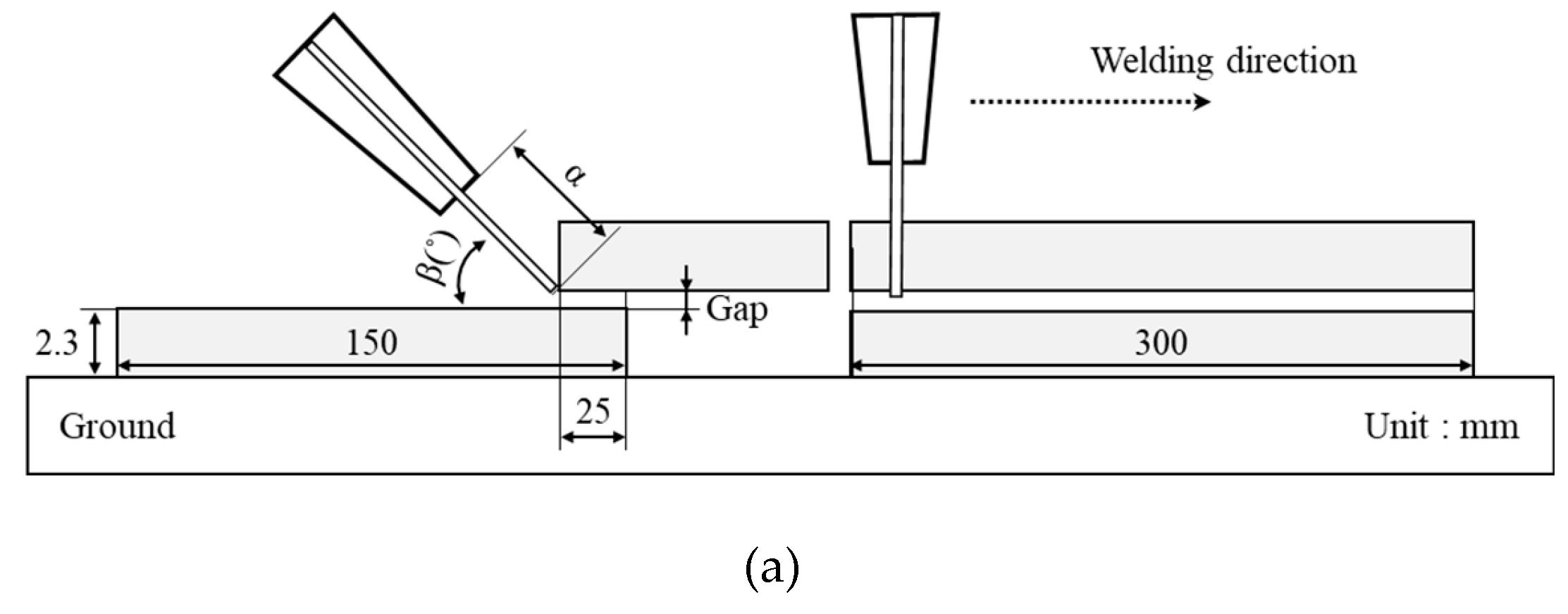
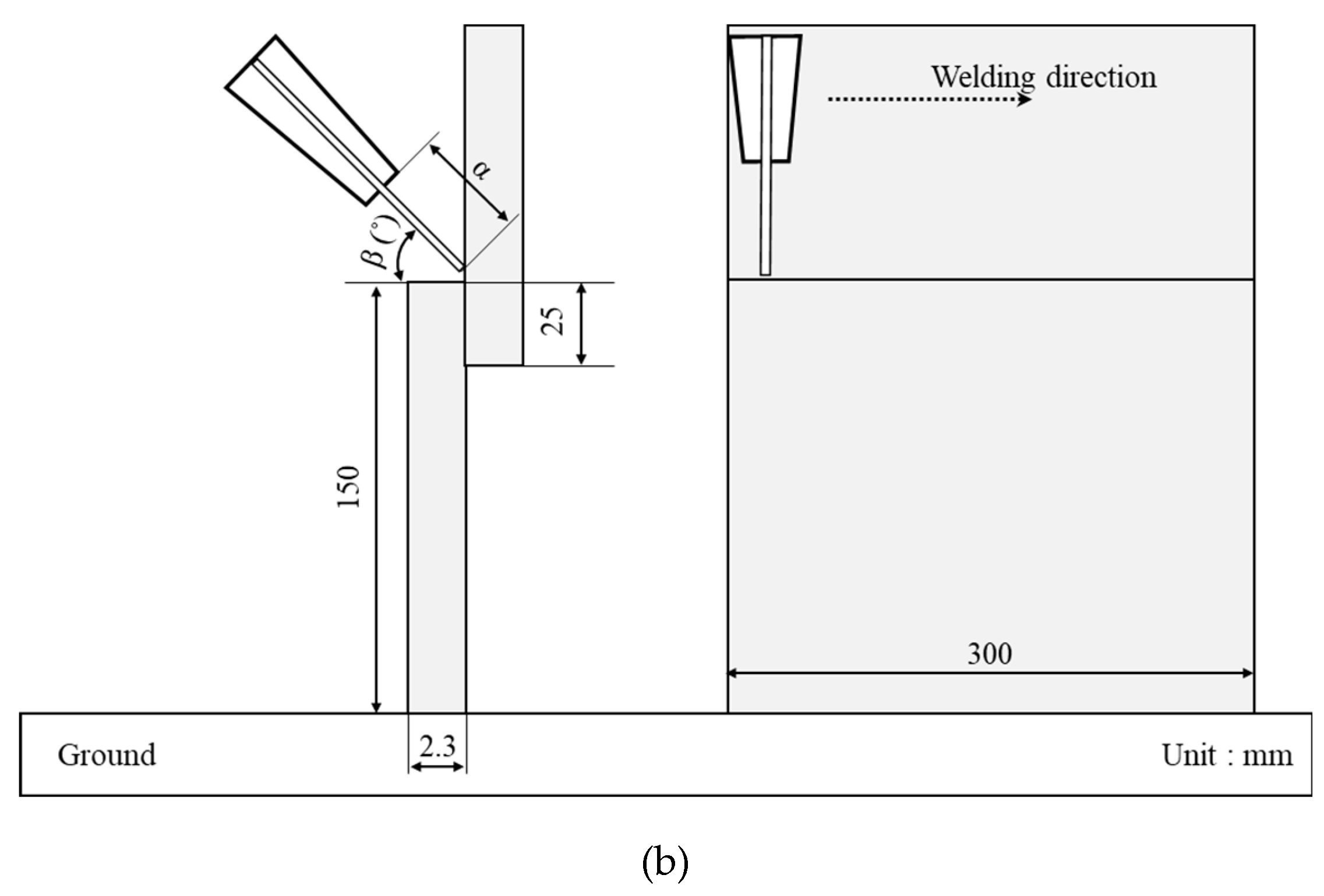
Figure 2.
Configuration of fatigue specimen.

Figure 3.
Amplitude fluctuations of the applied fatigue stress.

Figure 5.
Schematic to the definition of safety fatigue strength

Figure 4.
Schematic of weld joint geometry factors (a) length, (b) angle, (c) area.

Figure 6.
Fatigue behavior of lap joint weld by welding conditions (a) WFR variation (fixed B position, WP: DC, WS: 60 cm/min, gap: 0 mm), (b) WS variation (fixed A position, gap: 0 mm), (c) gap variation (fixed A position, WP: CMT, WFR: 5.0 m/min, WS: 80 cm/min), (d) position variation (fixed WFR: 5.0 m/min, WS: 60 cm/min, gap: 0 mm).
Figure 6.
Fatigue behavior of lap joint weld by welding conditions (a) WFR variation (fixed B position, WP: DC, WS: 60 cm/min, gap: 0 mm), (b) WS variation (fixed A position, gap: 0 mm), (c) gap variation (fixed A position, WP: CMT, WFR: 5.0 m/min, WS: 80 cm/min), (d) position variation (fixed WFR: 5.0 m/min, WS: 60 cm/min, gap: 0 mm).

Figure 7.
The relationship between (a)

Figure 8.
Hardness distribution of the lap weld according to heat input and gap.

Figure 9.
Relationship between measured value and estimated value by regression models (a)

| P-value | Step | |||||||
| #1 | #2 | #3 | #4 | #5 | #6 | #7 | #8 | |
| X1 | 0.62 | 0.61 | 0.60 | 0.24 | 0.10 | 0.07 | 0.07 | - |
| X2 | 0.59 | 0.53 | 0.52 | 0.52 | 0.53 | - | - | - |
| X3 | 0.78 | 0.74 | 0.73 | 0.83 | - | - | - | - |
| X4 | 0.02 | 0.00 | 0.00 | 0.00 | 0.00 | 0.00 | 0.00 | 0.00 |
| X5 | 0.37 | 0.25 | 0.24 | 0.20 | 0.18 | 0.09 | - | - |
| X7 | 0.10 | 0.09 | 0.08 | 0.08 | 0.06 | 0.06 | 0.03 | 0.01 |
| X8 | 0.97 | 0.97 | - | - | - | - | - | - |
| X9 | 0.80 | 0.78 | 0.78 | - | - | - | - | - |
| X10 | 0.01 | 0.00 | 0.01 | 0.00 | 0.00 | 0.00 | 0.00 | 0.00 |
| X13 | 0.98 | - | - | - | - | - | - | - |
| X14 | 0.00 | 0.00 | 0.00 | 0.00 | 0.00 | 0.00 | 0.00 | 0.00 |
| X16 | 0.23 | 0.02 | 0.02 | 0.02 | 0.10 | 0.00 | 0.00 | 0.00 |
| 0.84 | 0.84 | 0.84 | 0.84 | 0.85 | 0.85 | 0.84 | 0.84 | |
| 7.474 | 7.424 | 7.375 | 7.331 | 7.286 | 7.258 | 7.348 | 7.461 | |
| P-value | Step | |||||||
| #1 | #2 | #3 | #4 | #5 | #6 | #7 | #8 | |
| X1 | 0.20 | 0.20 | 0.21 | 0.16 | 0.11 | 0.18 | - | - |
| X2 | 0.73 | 0.74 | 0.83 | - | - | - | - | - |
| X3 | 0.35 | 0.34 | 0.33 | 0.29 | - | - | - | - |
| X4 | 0.07 | 0.06 | 0.01 | 0.00 | 0.00 | 0.00 | 0.00 | 0.00 |
| X5 | 0.24 | 0.24 | 0.19 | 0.11 | 0.10 | 0.09 | 0.14 | - |
| X7 | 0.83 | - | - | - | - | - | - | - |
| X8 | 0.26 | 0.23 | 0.24 | 0.23 | 0.19 | - | - | - |
| X9 | 0.05 | 0.05 | 0.04 | 0.01 | 0.01 | 0.03 | 0.03 | 0.03 |
| X10 | 0.00 | 0.00 | 0.00 | 0.00 | 0.00 | 0.00 | 0.00 | 0.00 |
| X13 | 0.075 | 0.76 | - | - | - | - | - | - |
| X14 | 0.00 | 0.00 | 0.00 | 0.00 | 0.00 | 0.00 | 0.00 | 0.00 |
| X16 | 0.11 | 0.10 | 0.11 | 0.08 | 0.00 | 0.00 | 0.00 | 0.00 |
| 0.86 | 0.86 | 0.86 | 0.86 | 0.86 | 0.86 | 0.86 | 0.86 | |
| 0.170 | 0.169 | 0.168 | 0.167 | 0.167 | 0.167 | 0.169 | 0.170 | |
| X1 | X2 | X3 | X4 | X5 | X6 | X7 | X8 | X9 | X10 | X11 | X12 | X13 | X14 | X15 | X16 | ||
| X1 | 0.76 | ||||||||||||||||
| X2 | 0.51 | 0.63 | |||||||||||||||
| X3 | 0.27 | 0.54 | 0.83 | ||||||||||||||
| X4 | -0.43 | -0.35 | 0.16 | 0.49 | |||||||||||||
| X5 | 0.78 | 0.60 | 0.36 | 0.07 | -0.46 | ||||||||||||
| X6 | 0.07 | 0.26 | 0.84 | 0.89 | 0.61 | -0.13 | |||||||||||
| X7 | 0.37 | 0.50 | 0.74 | 0.68 | 0.24 | 0.22 | 0.66 | ||||||||||
| X8 | 0.21 | 0.06 | 0.25 | 0.05 | 0.04 | 0.19 | 0.16 | 0.29 | |||||||||
| X9 | 0.69 | 0.88 | 0.27 | 0.26 | -0.56 | 0.58 | -0.13 | 0.21 | -0.11 | ||||||||
| X10 | -0.84 | -0.75 | -0.61 | -0.33 | 0.49 | -0.67 | -0.18 | -0.39 | -0.18 | -0.66 | |||||||
| X11 | -0.66 | -0.90 | -0.24 | -0.23 | 0.53 | -0.53 | 0.13 | -0.22 | 0.06 | -0.96 | 0.60 | ||||||
| X12 | 0.59 | 0.85 | 0.21 | 0.19 | -0.46 | 0.45 | -0.12 | 0.22 | -0.01 | 0.86 | -0.51 | -0.97 | |||||
| X13 | -0.67 | -0.55 | -0.07 | 0.31 | 0.92 | -0.74 | 0.47 | 0.04 | -0.09 | -0.68 | 0.66 | 0.63 | -0.55 | ||||
| X14 | 0.83 | 0.74 | 0.43 | 0.09 | -0.72 | 0.77 | -0.08 | 0.22 | 0.15 | 0.73 | -0.82 | -0.69 | 0.61 | -0.86 | |||
| X15 | 0.74 | 0.96 | 0.80 | 0.66 | -0.23 | 0.59 | 0.45 | 0.62 | 0.12 | 0.75 | -0.77 | -0.75 | 0.70 | -0.45 | 0.70 | ||
| X16 | -0.11 | 0.11 | 0.71 | 0.82 | 0.70 | -0.24 | 0.95 | 0.63 | 0.11 | -0.24 | 0.03 | 0.22 | -0.20 | 0.60 | -0.23 | 0.29 | |
| X17 | 0.33 | 0.47 | 0.80 | 0.76 | 0.32 | 0.16 | 0.77 | 0.98 | 0.27 | 0.15 | -0.39 | -0.16 | 0.15 | 0.12 | 0.18 | 0.62 | 0.74 |
| X1 | X2 | X3 | X4 | X5 | X6 | X7 | X8 | X9 | X10 | X11 | X12 | X13 | X14 | X15 | X16 | ||
| X1 | -0.66 | ||||||||||||||||
| X2 | -0.26 | 0.63 | |||||||||||||||
| X3 | -0.02 | 0.54 | 0.83 | ||||||||||||||
| X4 | 0.62 | -0.35 | 0.16 | 0.49 | |||||||||||||
| X5 | -0.77 | 0.60 | 0.36 | 0.07 | -0.46 | ||||||||||||
| X6 | 0.21 | 0.26 | 0.84 | 0.89 | 0.61 | -0.13 | |||||||||||
| X7 | -0.13 | 0.50 | 0.74 | 0.68 | 0.24 | 0.22 | 0.66 | ||||||||||
| X8 | -0.15 | 0.06 | 0.25 | 0.05 | 0.04 | 0.19 | 0.16 | 0.29 | |||||||||
| X9 | -0.73 | 0.88 | 0.27 | 0.26 | -0.56 | 0.58 | -0.13 | 0.21 | -0.11 | ||||||||
| X10 | 0.82 | -0.75 | -0.61 | -0.33 | 0.49 | -0.67 | -0.18 | -0.39 | -0.18 | -0.66 | |||||||
| X11 | 0.68 | -0.90 | -0.24 | -0.23 | 0.53 | -0.53 | 0.13 | -0.22 | 0.06 | -0.96 | 0.60 | ||||||
| X12 | -0.59 | 0.89 | 0.21 | 0.19 | -0.46 | 0.45 | -0.12 | 0.22 | -0.01 | 0.86 | -0.51 | -0.97 | |||||
| X13 | 0.79 | -0.55 | -0.07 | 0.31 | 0.92 | -0.74 | 0.47 | 0.04 | -0.09 | -0.68 | 0.66 | 0.63 | -0.55 | ||||
| X14 | -0.84 | 0.74 | 0.43 | 0.09 | -0.72 | 0.77 | -0.08 | 0.22 | 0.15 | 0.73 | -0.82 | -0.69 | 0.61 | -0.86 | |||
| X15 | -0.58 | 0.96 | 0.80 | 0.66 | -0.23 | 0.59 | 0.45 | 0.62 | 0.12 | 0.75 | -0.77 | -0.75 | 0.70 | -0.45 | 0.71 | ||
| X16 | 0.38 | 0.11 | 0.71 | 0.82 | 0.70 | -0.24 | 0.95 | 0.63 | 0.11 | -0.24 | 0.03 | 0.22 | -0.20 | 0.60 | -0.23 | 0.29 | |
| X17 | -0.07 | 0.47 | 0.80 | 0.76 | 0.31 | 0.16 | 0.77 | 0.98 | 0.27 | 0.15 | -0.39 | -0.16 | 0.15 | 0.12 | 0.18 | 0.62 | 0.74 |
Figure 10.
Stress distribution of lap welds during loading (a) stress distribution field, (b) bending morphology at weld toe and root stress concentration.
Figure 10.
Stress distribution of lap welds during loading (a) stress distribution field, (b) bending morphology at weld toe and root stress concentration.

| P-value | Step | |||||||
| #1 | #2 | #3 | #4 | #5 | #6 | #7 | #8 | |
| X1 | 0.62 | 0.61 | 0.60 | 0.24 | 0.10 | 0.07 | 0.07 | - |
| X2 | 0.59 | 0.53 | 0.52 | 0.52 | 0.53 | - | - | - |
| X3 | 0.78 | 0.74 | 0.73 | 0.83 | - | - | - | - |
| X4 | 0.02 | 0.00 | 0.00 | 0.00 | 0.00 | 0.00 | 0.00 | 0.00 |
| X5 | 0.37 | 0.25 | 0.24 | 0.20 | 0.18 | 0.09 | - | - |
| X7 | 0.10 | 0.09 | 0.08 | 0.08 | 0.06 | 0.06 | 0.03 | 0.01 |
| X8 | 0.97 | 0.97 | - | - | - | - | - | - |
| X9 | 0.80 | 0.78 | 0.78 | - | - | - | - | - |
| X10 | 0.01 | 0.00 | 0.01 | 0.00 | 0.00 | 0.00 | 0.00 | 0.00 |
| X13 | 0.98 | - | - | - | - | - | - | - |
| X14 | 0.00 | 0.00 | 0.00 | 0.00 | 0.00 | 0.00 | 0.00 | 0.00 |
| X16 | 0.23 | 0.02 | 0.02 | 0.02 | 0.10 | 0.00 | 0.00 | 0.00 |
| 0.84 | 0.84 | 0.84 | 0.84 | 0.85 | 0.85 | 0.84 | 0.84 | |
| 7.474 | 7.424 | 7.375 | 7.331 | 7.286 | 7.258 | 7.348 | 7.461 | |
| P-value | Step | |||||||
| #1 | #2 | #3 | #4 | #5 | #6 | #7 | #8 | |
| X1 | 0.20 | 0.20 | 0.21 | 0.16 | 0.11 | 0.18 | - | - |
| X2 | 0.73 | 0.74 | 0.83 | - | - | - | - | - |
| X3 | 0.35 | 0.34 | 0.33 | 0.29 | - | - | - | - |
| X4 | 0.07 | 0.06 | 0.01 | 0.00 | 0.00 | 0.00 | 0.00 | 0.00 |
| X5 | 0.24 | 0.24 | 0.19 | 0.11 | 0.10 | 0.09 | 0.14 | - |
| X7 | 0.83 | - | - | - | - | - | - | - |
| X8 | 0.26 | 0.23 | 0.24 | 0.23 | 0.19 | - | - | - |
| X9 | 0.05 | 0.05 | 0.04 | 0.01 | 0.01 | 0.03 | 0.03 | 0.03 |
| X10 | 0.00 | 0.00 | 0.00 | 0.00 | 0.00 | 0.00 | 0.00 | 0.00 |
| X13 | 0.075 | 0.76 | - | - | - | - | - | - |
| X14 | 0.00 | 0.00 | 0.00 | 0.00 | 0.00 | 0.00 | 0.00 | 0.00 |
| X16 | 0.11 | 0.10 | 0.11 | 0.08 | 0.00 | 0.00 | 0.00 | 0.00 |
| 0.86 | 0.86 | 0.86 | 0.86 | 0.86 | 0.86 | 0.86 | 0.86 | |
| 0.170 | 0.169 | 0.168 | 0.167 | 0.167 | 0.167 | 0.169 | 0.170 | |
| X1 | X2 | X3 | X4 | X5 | X6 | X7 | X8 | X9 | X10 | X11 | X12 | X13 | X14 | X15 | X16 | ||
| X1 | 0.76 | ||||||||||||||||
| X2 | 0.51 | 0.63 | |||||||||||||||
| X3 | 0.27 | 0.54 | 0.83 | ||||||||||||||
| X4 | -0.43 | -0.35 | 0.16 | 0.49 | |||||||||||||
| X5 | 0.78 | 0.60 | 0.36 | 0.07 | -0.46 | ||||||||||||
| X6 | 0.07 | 0.26 | 0.84 | 0.89 | 0.61 | -0.13 | |||||||||||
| X7 | 0.37 | 0.50 | 0.74 | 0.68 | 0.24 | 0.22 | 0.66 | ||||||||||
| X8 | 0.21 | 0.06 | 0.25 | 0.05 | 0.04 | 0.19 | 0.16 | 0.29 | |||||||||
| X9 | 0.69 | 0.88 | 0.27 | 0.26 | -0.56 | 0.58 | -0.13 | 0.21 | -0.11 | ||||||||
| X10 | -0.84 | -0.75 | -0.61 | -0.33 | 0.49 | -0.67 | -0.18 | -0.39 | -0.18 | -0.66 | |||||||
| X11 | -0.66 | -0.90 | -0.24 | -0.23 | 0.53 | -0.53 | 0.13 | -0.22 | 0.06 | -0.96 | 0.60 | ||||||
| X12 | 0.59 | 0.85 | 0.21 | 0.19 | -0.46 | 0.45 | -0.12 | 0.22 | -0.01 | 0.86 | -0.51 | -0.97 | |||||
| X13 | -0.67 | -0.55 | -0.07 | 0.31 | 0.92 | -0.74 | 0.47 | 0.04 | -0.09 | -0.68 | 0.66 | 0.63 | -0.55 | ||||
| X14 | 0.83 | 0.74 | 0.43 | 0.09 | -0.72 | 0.77 | -0.08 | 0.22 | 0.15 | 0.73 | -0.82 | -0.69 | 0.61 | -0.86 | |||
| X15 | 0.74 | 0.96 | 0.80 | 0.66 | -0.23 | 0.59 | 0.45 | 0.62 | 0.12 | 0.75 | -0.77 | -0.75 | 0.70 | -0.45 | 0.70 | ||
| X16 | -0.11 | 0.11 | 0.71 | 0.82 | 0.70 | -0.24 | 0.95 | 0.63 | 0.11 | -0.24 | 0.03 | 0.22 | -0.20 | 0.60 | -0.23 | 0.29 | |
| X17 | 0.33 | 0.47 | 0.80 | 0.76 | 0.32 | 0.16 | 0.77 | 0.98 | 0.27 | 0.15 | -0.39 | -0.16 | 0.15 | 0.12 | 0.18 | 0.62 | 0.74 |
| X1 | X2 | X3 | X4 | X5 | X6 | X7 | X8 | X9 | X10 | X11 | X12 | X13 | X14 | X15 | X16 | ||
| X1 | -0.66 | ||||||||||||||||
| X2 | -0.26 | 0.63 | |||||||||||||||
| X3 | -0.02 | 0.54 | 0.83 | ||||||||||||||
| X4 | 0.62 | -0.35 | 0.16 | 0.49 | |||||||||||||
| X5 | -0.77 | 0.60 | 0.36 | 0.07 | -0.46 | ||||||||||||
| X6 | 0.21 | 0.26 | 0.84 | 0.89 | 0.61 | -0.13 | |||||||||||
| X7 | -0.13 | 0.50 | 0.74 | 0.68 | 0.24 | 0.22 | 0.66 | ||||||||||
| X8 | -0.15 | 0.06 | 0.25 | 0.05 | 0.04 | 0.19 | 0.16 | 0.29 | |||||||||
| X9 | -0.73 | 0.88 | 0.27 | 0.26 | -0.56 | 0.58 | -0.13 | 0.21 | -0.11 | ||||||||
| X10 | 0.82 | -0.75 | -0.61 | -0.33 | 0.49 | -0.67 | -0.18 | -0.39 | -0.18 | -0.66 | |||||||
| X11 | 0.68 | -0.90 | -0.24 | -0.23 | 0.53 | -0.53 | 0.13 | -0.22 | 0.06 | -0.96 | 0.60 | ||||||
| X12 | -0.59 | 0.89 | 0.21 | 0.19 | -0.46 | 0.45 | -0.12 | 0.22 | -0.01 | 0.86 | -0.51 | -0.97 | |||||
| X13 | 0.79 | -0.55 | -0.07 | 0.31 | 0.92 | -0.74 | 0.47 | 0.04 | -0.09 | -0.68 | 0.66 | 0.63 | -0.55 | ||||
| X14 | -0.84 | 0.74 | 0.43 | 0.09 | -0.72 | 0.77 | -0.08 | 0.22 | 0.15 | 0.73 | -0.82 | -0.69 | 0.61 | -0.86 | |||
| X15 | -0.58 | 0.96 | 0.80 | 0.66 | -0.23 | 0.59 | 0.45 | 0.62 | 0.12 | 0.75 | -0.77 | -0.75 | 0.70 | -0.45 | 0.71 | ||
| X16 | 0.38 | 0.11 | 0.71 | 0.82 | 0.70 | -0.24 | 0.95 | 0.63 | 0.11 | -0.24 | 0.03 | 0.22 | -0.20 | 0.60 | -0.23 | 0.29 | |
| X17 | -0.07 | 0.47 | 0.80 | 0.76 | 0.31 | 0.16 | 0.77 | 0.98 | 0.27 | 0.15 | -0.39 | -0.16 | 0.15 | 0.12 | 0.18 | 0.62 | 0.74 |

Table 1.
Welding parameter.
| Chemical composition [wt.%] | Mechanical properties | |||||||
| C | Si | Mn | P | S | TS [MPa]* | YS [MPa]* | EL [%] * | |
| Base material | 0.07 | 0.14 | 1.44 | 0.13 | 0.002 | 610 | 583 | 25 |
| Filler wire | 0.07 | 0.65 | 1.14 | 0.02 | 0.010 | 560 | 440 | 28 |
* Note. TS: Tensile strength, YS: Yield strength, EL: Elongation.
Table 2.
Welding processes and conditions.
| Parameters | Value | |||
| Weld joint | A position | B position | ||
| WP | CMT | DC | CMT | DC |
| WFR (m/min) | 5.0, 7.0, 9.0 | 3.0, 5.0, 7.0 | 5.0, 7.0, 9.0 | 3.0, 5.0, 7.0 |
| WS (cm/min) | 60, 80 | |||
| Gap (mm) | 0, 0.2, 0.5, 1.0 | |||
| CTWD (α, mm) | 15 | |||
| Work angle (β, ˚) | 45 | |||
| Shielding gas | 90 % Ar + 10% CO2 (25 L/min) | |||
Table 3.
Fatigue test conditions.
| Maximum stress() | 366–122 MPa (at intervals of 10 %) |
| 122–62 MPa (at intervals of 5 %) | |
| 62 MPa under (at intervals of 2.5 %) | |
| Stress ratio (R) | 0.1 |
| Frequency | 40 Hz |
| Fatigue limit | 2 × 10⁶ cycles |
Table 5.
Correlation matrix between the independent variables and
| X1 | X2 | X3 | X4 | X5 | X6 | X7 | X8 | X9 | X10 | X11 | X12 | X13 | X14 | X15 | X16 | ||
| X1 | -0.66 | ||||||||||||||||
| X2 | -0.26 | 0.63 | |||||||||||||||
| X3 | -0.02 | 0.54 | 0.83 | ||||||||||||||
| X4 | 0.62 | -0.35 | 0.16 | 0.49 | |||||||||||||
| X5 | -0.77 | 0.60 | 0.36 | 0.07 | -0.46 | ||||||||||||
| X6 | 0.21 | 0.26 | 0.84 | 0.89 | 0.61 | -0.13 | |||||||||||
| X7 | -0.13 | 0.50 | 0.74 | 0.68 | 0.24 | 0.22 | 0.66 | ||||||||||
| X8 | -0.15 | 0.06 | 0.25 | 0.05 | 0.04 | 0.19 | 0.16 | 0.29 | |||||||||
| X9 | -0.73 | 0.88 | 0.27 | 0.26 | -0.56 | 0.58 | -0.13 | 0.21 | -0.11 | ||||||||
| X10 | 0.82 | -0.75 | -0.61 | -0.33 | 0.49 | -0.67 | -0.18 | -0.39 | -0.18 | -0.66 | |||||||
| X11 | 0.68 | -0.90 | -0.24 | -0.23 | 0.53 | -0.53 | 0.13 | -0.22 | 0.06 | -0.96 | 0.60 | ||||||
| X12 | -0.59 | 0.89 | 0.21 | 0.19 | -0.46 | 0.45 | -0.12 | 0.22 | -0.01 | 0.86 | -0.51 | -0.97 | |||||
| X13 | 0.79 | -0.55 | -0.07 | 0.31 | 0.92 | -0.74 | 0.47 | 0.04 | -0.09 | -0.68 | 0.66 | 0.63 | -0.55 | ||||
| X14 | -0.84 | 0.74 | 0.43 | 0.09 | -0.72 | 0.77 | -0.08 | 0.22 | 0.15 | 0.73 | -0.82 | -0.69 | 0.61 | -0.86 | |||
| X15 | -0.58 | 0.96 | 0.80 | 0.66 | -0.23 | 0.59 | 0.45 | 0.62 | 0.12 | 0.75 | -0.77 | -0.75 | 0.70 | -0.45 | 0.71 | ||
| X16 | 0.38 | 0.11 | 0.71 | 0.82 | 0.70 | -0.24 | 0.95 | 0.63 | 0.11 | -0.24 | 0.03 | 0.22 | -0.20 | 0.60 | -0.23 | 0.29 | |
| X17 | -0.07 | 0.47 | 0.80 | 0.76 | 0.31 | 0.16 | 0.77 | 0.98 | 0.27 | 0.15 | -0.39 | -0.16 | 0.15 | 0.12 | 0.18 | 0.62 | 0.74 |
Table 6.
Correlation matrix between the independent variables and
| X1 | X2 | X3 | X4 | X5 | X6 | X7 | X8 | X9 | X10 | X11 | X12 | X13 | X14 | X15 | X16 | ||
| X1 | 0.76 | ||||||||||||||||
| X2 | 0.51 | 0.63 | |||||||||||||||
| X3 | 0.27 | 0.54 | 0.83 | ||||||||||||||
| X4 | -0.43 | -0.35 | 0.16 | 0.49 | |||||||||||||
| X5 | 0.78 | 0.60 | 0.36 | 0.07 | -0.46 | ||||||||||||
| X6 | 0.07 | 0.26 | 0.84 | 0.89 | 0.61 | -0.13 | |||||||||||
| X7 | 0.37 | 0.50 | 0.74 | 0.68 | 0.24 | 0.22 | 0.66 | ||||||||||
| X8 | 0.21 | 0.06 | 0.25 | 0.05 | 0.04 | 0.19 | 0.16 | 0.29 | |||||||||
| X9 | 0.69 | 0.88 | 0.27 | 0.26 | -0.56 | 0.58 | -0.13 | 0.21 | -0.11 | ||||||||
| X10 | -0.84 | -0.75 | -0.61 | -0.33 | 0.49 | -0.67 | -0.18 | -0.39 | -0.18 | -0.66 | |||||||
| X11 | -0.66 | -0.90 | -0.24 | -0.23 | 0.53 | -0.53 | 0.13 | -0.22 | 0.06 | -0.96 | 0.60 | ||||||
| X12 | 0.59 | 0.85 | 0.21 | 0.19 | -0.46 | 0.45 | -0.12 | 0.22 | -0.01 | 0.86 | -0.51 | -0.97 | |||||
| X13 | -0.67 | -0.55 | -0.07 | 0.31 | 0.92 | -0.74 | 0.47 | 0.04 | -0.09 | -0.68 | 0.66 | 0.63 | -0.55 | ||||
| X14 | 0.83 | 0.74 | 0.43 | 0.09 | -0.72 | 0.77 | -0.08 | 0.22 | 0.15 | 0.73 | -0.82 | -0.69 | 0.61 | -0.86 | |||
| X15 | 0.74 | 0.96 | 0.80 | 0.66 | -0.23 | 0.59 | 0.45 | 0.62 | 0.12 | 0.75 | -0.77 | -0.75 | 0.70 | -0.45 | 0.70 | ||
| X16 | -0.11 | 0.11 | 0.71 | 0.82 | 0.70 | -0.24 | 0.95 | 0.63 | 0.11 | -0.24 | 0.03 | 0.22 | -0.20 | 0.60 | -0.23 | 0.29 | |
| X17 | 0.33 | 0.47 | 0.80 | 0.76 | 0.32 | 0.16 | 0.77 | 0.98 | 0.27 | 0.15 | -0.39 | -0.16 | 0.15 | 0.12 | 0.18 | 0.62 | 0.74 |
Table 7.
Significance provability values of regression coefficients for the back elimination method and its result for
Table 7.
Significance provability values of regression coefficients for the back elimination method and its result for
| P-value | Step | |||||||
| #1 | #2 | #3 | #4 | #5 | #6 | #7 | #8 | |
| X1 | 0.20 | 0.20 | 0.21 | 0.16 | 0.11 | 0.18 | - | - |
| X2 | 0.73 | 0.74 | 0.83 | - | - | - | - | - |
| X3 | 0.35 | 0.34 | 0.33 | 0.29 | - | - | - | - |
| X4 | 0.07 | 0.06 | 0.01 | 0.00 | 0.00 | 0.00 | 0.00 | 0.00 |
| X5 | 0.24 | 0.24 | 0.19 | 0.11 | 0.10 | 0.09 | 0.14 | - |
| X7 | 0.83 | - | - | - | - | - | - | - |
| X8 | 0.26 | 0.23 | 0.24 | 0.23 | 0.19 | - | - | - |
| X9 | 0.05 | 0.05 | 0.04 | 0.01 | 0.01 | 0.03 | 0.03 | 0.03 |
| X10 | 0.00 | 0.00 | 0.00 | 0.00 | 0.00 | 0.00 | 0.00 | 0.00 |
| X13 | 0.075 | 0.76 | - | - | - | - | - | - |
| X14 | 0.00 | 0.00 | 0.00 | 0.00 | 0.00 | 0.00 | 0.00 | 0.00 |
| X16 | 0.11 | 0.10 | 0.11 | 0.08 | 0.00 | 0.00 | 0.00 | 0.00 |
| 0.86 | 0.86 | 0.86 | 0.86 | 0.86 | 0.86 | 0.86 | 0.86 | |
| 0.170 | 0.169 | 0.168 | 0.167 | 0.167 | 0.167 | 0.169 | 0.170 | |
Table 8.
Significance provability values of regression coefficients for the back elimination method and its result for
Table 8.
Significance provability values of regression coefficients for the back elimination method and its result for
| P-value | Step | |||||||
| #1 | #2 | #3 | #4 | #5 | #6 | #7 | #8 | |
| X1 | 0.62 | 0.61 | 0.60 | 0.24 | 0.10 | 0.07 | 0.07 | - |
| X2 | 0.59 | 0.53 | 0.52 | 0.52 | 0.53 | - | - | - |
| X3 | 0.78 | 0.74 | 0.73 | 0.83 | - | - | - | - |
| X4 | 0.02 | 0.00 | 0.00 | 0.00 | 0.00 | 0.00 | 0.00 | 0.00 |
| X5 | 0.37 | 0.25 | 0.24 | 0.20 | 0.18 | 0.09 | - | - |
| X7 | 0.10 | 0.09 | 0.08 | 0.08 | 0.06 | 0.06 | 0.03 | 0.01 |
| X8 | 0.97 | 0.97 | - | - | - | - | - | - |
| X9 | 0.80 | 0.78 | 0.78 | - | - | - | - | - |
| X10 | 0.01 | 0.00 | 0.01 | 0.00 | 0.00 | 0.00 | 0.00 | 0.00 |
| X13 | 0.98 | - | - | - | - | - | - | - |
| X14 | 0.00 | 0.00 | 0.00 | 0.00 | 0.00 | 0.00 | 0.00 | 0.00 |
| X16 | 0.23 | 0.02 | 0.02 | 0.02 | 0.10 | 0.00 | 0.00 | 0.00 |
| 0.84 | 0.84 | 0.84 | 0.84 | 0.85 | 0.85 | 0.84 | 0.84 | |
| 7.474 | 7.424 | 7.375 | 7.331 | 7.286 | 7.258 | 7.348 | 7.461 | |
Table 9.
Standardized regression coefficients of the
Table 10.
Standardized regression coefficients of the
Table 11.
Coefficient of determination and standard error of the estimate for the
Table 12.
Coefficient of determination and standard error of the estimate for the
Disclaimer/Publisher’s Note: The statements, opinions and data contained in all publications are solely those of the individual author(s) and contributor(s) and not of MDPI and/or the editor(s). MDPI and/or the editor(s) disclaim responsibility for any injury to people or property resulting from any ideas, methods, instructions or products referred to in the content. |
© 2024 by the authors. Licensee MDPI, Basel, Switzerland. This article is an open access article distributed under the terms and conditions of the Creative Commons Attribution (CC BY) license (http://creativecommons.org/licenses/by/4.0/).
Copyright: This open access article is published under a Creative Commons CC BY 4.0 license, which permit the free download, distribution, and reuse, provided that the author and preprint are cited in any reuse.


