Submitted:
18 August 2024
Posted:
19 August 2024
You are already at the latest version
Abstract
This paper presents a dynamic homotopy technique that can be used to calculate a preliminary result for a power flow problem (PFP). This result can then be used as an initial estimate to efficiently solve the PFP using either the classical Newton-Raphson (NR) method or its fast decoupled version (FDXB) while still maintaining high accuracy. The preliminary stage for the dynamic homotopy problem is formulated and solved by employing integration techniques, where implicit and explicit schemes are studied. The dynamic problem assumes an initial condition that coincides with the initial estimate for a traditional iterative method such as NR. In this sense, the initial guess for the FPF is adequately set as a flat start, which is a starting for the case when this initialization is of difficult assignment for convergence. The static homotopy method requires a complete solution of a PFP per homotopy pathway point, while the dynamic homotopy is based on numerical integration methods. This approach can require only one LU factorization at each point of the pathway. Allocating these points properly helps avoid several PFP resolutions to build the pathway. The hybrid technique was evaluated for large-scale systems with poor conditioning, such as a 109272-bus model and other test systems under stressed conditions. A scheme based on the implicit backward Euler scheme demonstrated the best performance among other numerical solvers studied. It provided reliable partial results for the dynamic homotopy problem, which proved to be suitable for achieving fast and highly accurate solutions using both the NR and FDXB solvers.
Keywords:
Dynamic homotopy
; Newton-Raphson method
; integration method
; backward Euler scheme
; fast decoupled Newton-Raphson
; ill-conditioned system
1. Introduction
The power flow computational tool is necessary to determine the operating point of an electrical grid. This nonlinear problem has been widely studied for a long time. Currently, it can involve large-scale, sometimes poorly conditioned systems, which can constantly change in some form depending on the grid conditions. More recent physical aspects that contribute to this change include the presence of new types of energy sources and the configuration of the grid to meet certain operational states. In this sense, research into robust computational techniques to solve the problem becomes attractive.
The main method for solving the power flow problem (PFP) is the iterative Newton-Raphson (NR) method and its variations, such as decoupled and fast decoupled techniques [1]. However, solving the resulting nonlinear problem can be challenging due to the difficulty in assigning the initial estimate. If the assignment is not properly defined, the problem might experience divergence or yield impractical results. Flat start initial estimation for the profile of electrical networks is a common strategy when precise knowledge of the system’s operating point is difficult to obtain [1]. This is a more realistic situation nowadays due to changes caused by events such as the diversified load profile and the integration of intermittent renewable sources [2,3,4], among other factors [5,6]. In certain cases, particularly in large networks, using flat start PFP initialization may cause the problem to diverge [7]. According to [8], when this numerical detail is identified, it does not necessarily mean that the problem has no solution. i.e., if a solution exists, the problem is considered ill-conditioned, and finding the solution using traditional iterative techniques is challenging.
Investigations on the ill-conditioned topic applied to power system models have long been of interest [9]. However, in recent years numerous studies on the subject have been published [7,8,10,11,12,13,14]. Furthermore, there exist various methodologies proposing a way to solve the nonlinear problem embedded in the PFP.
A dynamic approach from the PFP power balance equations was investigated in [8] after the original problem was converted into a set of Ordinary Differential Equations (ODEs). In a first approach, the dynamic problem was solved using an explicit integration method [8]. Later on, the same problem was readdressed and resolved using an implicit method [7]. In these cases, the classical methods of Euler and Runge-Kutta were explored. Given the simplicity of these numerical integration techniques, other forms were investigated by other researchers [10,15]. The method developed in [10] considered the study of well- and ill-conditioned electrical systems models using a technique denominated Heun-King-Werner (HKW) method. The HKW method presented superior efficiency and convergence performance compared to conventional PFP solution methods. The classical Newton-Raphson method often struggles to converge when dealing with ill-conditioned systems, unless specific parameters and/or initializations are used. This dependency on certain conditions makes the convergence highly insecure for using the Newton-Raphson method or other alternatives.
Methods based on homotopy have also been recently developed, in contrast to the previously mentioned fictitious dynamic techniques [11,13]. The problem involves calculating a PFP solution along a homotopy pathway until its final point using the NR solver. Changes in the homotopy parameter along the pathway result in solving the problem, which finally is concluded when the homotopy parameter reaches a value of one. Hence, the way an algorithm is implemented along the homotopy path differs for each technique. For instance, in [13], the homotopy technique is applied in analogy with components of electric circuits to simulate the nonlinear equations of the power balance equations. The publication exploits a static homotopy approach to calculating the PFP solution along the homotopy pathway. In the study [11], the static homotopy problem for the original PFP power balance equations is solved in a different way. As the homotopy parameter increases, the grid is transformed from a fictitious and decoupled bus power system to the original problem. This later state occurs when the homotopy parameter reaches unity. In [16], the continuation homotopy technique is applied for tracing curves and determining isolated solutions to the PFP. Some publications on homotopy techniques were also applied to the power flow problem in distribution systems [17,18]. Other applications are found to calculate Optimal Power Flow (OPF) [19] and for post-contingency actions as those ones verified in stressed network [20].
In the previous discussion of homotopy techniques, it was mentioned that solving the power balance equations is crucial at each point along the homotopy pathway. This procedure involves iterations at each point, especially when using the NR method. However, it is important to note that each NR iteration requires an LU factorization of the Jacobian matrix, which is computationally costly in PFP. Typically, at least three iterations are needed to achieve acceptable PFP convergence at a specific point along the homotopy pathway. If the partial PFP results along the homotopy path could be relaxed, it would save computational time until reaching the path’s endpoint, which defines the PFP solution. So, the challenge would be to reduce the computational burden associated with this problem or investigate an alternative solution for the PFP in this direction. A trial of reducing the computational burden was proposed in [21] by applying a strategy based on a dynamic homotopy [22] instead of a static one. In the publication [21], an approximation of the PFP solution is generated using a transient-based method. This approximation, combined with the classical NR solver, is employed to obtain a high-accuracy solution of the PFP. However, the technique and results require further in-depth studies.
This paper presents a dynamic homotopy-based approach, together with classical iterative techniques, to compute the solution of the PFP. Based on this technique, in combination with the NR method or still, its simplified version called fast decoupled NR (FDXB), high-accuracy solutions for the PFP are obtained. The dynamic homotopy problem, as formulated in [21] and based on [22], was extended in this paper to investigate in-depth and implement explicit integration techniques, such as forward Euler and second-order Runge-Kutta, and an implicit integration technique based on the backward Euler scheme. The dynamic homotopy structure allows the original PFP to be initialized from a flat starting estimate. The problem formulation describes how a simple homotopy function using a fixed point structure was implemented. This procedure introduces a proportional term, which, as shown in this proposed paper, is associated with a perturbation to remove or improve the numerical conditioning of the Jacobian matrix in the PFP (as suggested in [23]). The simulations show that the implicit method adequately provides an initial estimate for the NR and FDXB solvers. Furthermore, as formulated, it only requires one LU factorization for a dynamic homotopy pathway approximation point and allows for high integration steps. To demonstrate the effectiveness of the results obtained in the investigations, simulations are conducted in poorly conditioned systems and networks under stressful operating conditions. The simulations are performed in large-scale systems, including a grid with more than 109k buses.
Some contributions are identified as follows:
- Presentation of a technique enabling the use of the NR and FDXB solvers, demonstrating their efficiency despite starting from a flat initial guess;
- Demonstration that the dynamic homotopy problem for the PFP can be transformed into a fixed-point function, where the proportional term multiplying this function is associated with the original Jacobian PF;
- Use of the result obtained from the dynamic homotopy directly to execute the native scripts for NR and FDXB in the MATPOWER software [24]; and
- Investigations of explicit and implicit integration techniques to solve the dynamic homotopy problem efficiently.
The paper is structured as follows: Section 2 was dedicated to succinctly presenting the fundamentals required for the basic definitions found in the PFP, including the presentation of some solvers. In Section 3, the homotopy problem is presented and then the dynamic homotopy problem is formulated. In this section, the problem associated with the fixed-point inclusion is described, and also a generic tutorial example is introduced. Tests with several experiments and discussions of results are presented in Section 4. The main conclusions of the paper are described in Section 5.
2. Fundamentals of the Iterative Power flow
A power system is typically described by power balance equations (PBEs), a set of nonlinear equations governing the system. Well-accepted modeling is presented as a set of equations representing the power flow entering (leaving) a bus, using a voltage polar representation. These equations can be generalized for a total of buses by (1) for PQ- and PV-type, and (2) for PV-type, where the load buses and generation buses are named as PQ- and PV-type, respectively.
The variable to be determined is the voltage phasor, at a generic bus k, given by . According to the phasor notation, is the voltage magnitude, while is the phase angle. The power flow is represented by equations requiring the contribution of branches and shunt admittances. These admittances are organized in the form of an admittance matrix, , whose entries are given by . The net specified power injected into the bus k is given by to active power and to reactive power. Both and can assume voltage-dependent expressions [1] that are arranged into an exponential or a polynomial form, being the latter representation well-known as ZIP model. This work uses the representation from the MATPOWER framework, consisting of constant power and constant impedance, as available in the framework’s databank.
In addition to the buses PQ and PV, the system was modeled with only one slack bus. Hence, the total number of buses in the system is given by and the total number of Equations (1)–(2) is given by . Therefore, to solve the problem, it is sufficient to find the roots of the power balance equations. This set of equations can be generically represented by and the solution can be given by where is the network state vector and is a map of the type , defining the mismatches (residues) of the PBEs.
2.1. Traditional numerical solvers
The PBEs can be solved by iterative numerical methods starting from an initial estimate [25]. The iterative methods are characterized by increments and the objective is to find the root of the equation by using an appropriate root-finder. The initial estimate converge along the iteration to the root when , for sufficiently small, a given tolerance. Usually, the number of iterations is limited, and the method is interrupted if a given threshold is exceeded. PBEPower Balance Equation
Different methods proposed in the literature can solve the PBE [25]. Techniques such as Gauss-Seidel (GS) [25], and Newton-Raphson (NR) [1,26] are capable of numerically solving PBEs with different characteristics such as computation burden and number of iterations. The NR method stands out for presenting quadratic convergence when the initial voltage estimate is within the region of attraction. For this reason, it is widely used as a reference for performance analysis of numerical solvers.
2.1.1. Classical Newton-Raphson Method
The Newton-Raphson method is a classical technique used to solve the PBE [26]. It starts by using Taylor’s series expansions to approximate nonlinear functions while avoiding higher-order terms [27]. From the initial estimate , the solution is incremented through the mismatches of the previous iteration to reach a more accurate solution . Knowing that the Jacobian matrix for and is , when it is nonsingular, the iterative solution of the NR scheme can be summarized as
Nonstandard iterative techniques can be found in the literature, for example, those referred to as Newton’s Continuous (NC) type [7,8]. This methodology was inspired by the discrete iterative response in the process resolution carried out for a solution of an Ordinary Differential Equation (ODE) with a continuous parameter t. As a result, the ODE is represented by . Now, it can be solved by a traditional numerical integration method considering a time-step .
Some traditional integration techniques are briefly described in the sequence, considering the embedding of the PFP formulation.
2.1.2. Solution by Using a Standard Integration Method
The well-known numerical integration forward Euler (FE) method was adapted as a tool to solve the PFP in [8]. The static problem was converted to a “dynamic form” assuming a time-step . Note that the traditional NR method is identified if . An iteration scheme of the FE, for a starting-time is given by
In (4), the initial estimate for the static NR is also the initial condition for the ODE.
Since the FE is an explicit integration method, its performance when dealing with ill-conditioned systems in general has an aspect unfavorable. Therefore, an implicit scheme is more adequate. Exploiting this characteristic, a backward Euler (BE) type solver was proposed in [7]. The standard scheme for the BE is
In (5) the upgrade of the state variable, depends on the resolution of a nonlinear equation , where is unknown and is given. When dealing with large-scale problems the resolution of the nonlinear algebraic equation is not straightforward. In [7], it was presented some schemes to obtain a solution of this equation, including simplification aspects.
Techniques considering an aspect of predictor-corrector scheme are also found in the literature. It is important to consider that as the scheme becomes more complex, the computational workload to determine a single discrete value for the ODE can increase. This is due to the fact that each evaluation of the function requires the inversion of a Jacobian matrix.
Numerical schemes based on Runge-Kutta method families were also published in [8]. Similarly to the FE method, the Runge-Kutta formulas are explicit integration methods. However, depending on its adopted order, it will require more evaluations of the function . The solver requires additional computation expressed by constants for the same iterate. The second-order Runge-Kutta (RK2) iterative formula is given by
where the constants are calculated as , and ; is a fictitious time related to the iterations, generally not used explicitly in the formulas.
2.1.3. Runge-Kutta Fourth-Order Method
A classical RK4 is an efficient explicit numerical integration to solve the PBE using the previous state to take the next iteration and get the solution to the problem [8]. The update is composed of previous iteration results ang calculated as
where the constants are calculated as , , , and .
2.2. The Limitation of Traditional Methods
Traditional methods can have difficulty with convergence in practical power systems, especially in large-scale systems. For instance, techniques like Gauss-Seidel (GS), used to initialize the NR solver in some production-grade software, may experience slow convergence or be impractical in complex systems. Additionally, these methods may diverge or fail to find the appropriate solution under high loading levels. The Newton-Raphson (NR) method converges quadratically for initial estimates within the attraction region [26]. This can be crucial in situations where the region is narrow. Ideally, we need a robust method to search for the solution even when starting points are far from the solution.
During a real emergency, the network’s condition can change so much that a traditional estimate-based approach may not be enough to locate the new operating point using a power flow solver. Therefore, it is important to develop solvers for large-scale systems that can work independently of the initial voltage estimate, for example, by starting from a flat voltage start guess.
2.3. The Homotopy Method
Considering a network scenario, previously known initial estimates may not be sufficient for the convergence of a PFP. The homotopy method can build a controlled path towards convergence in this context, working as a tool to solve nonlinear equations and find the roots of [17,28,29]. In the homotopy path, the intermediate results are used as initial estimates for the computation of states in the following points. So, it is possible to build a path coordinated by parameters until the final equilibrium state, characterizing the original problem solution. In fact, through a parameter h, the problem of a “difficult” solution at is modeled for a system of an “easy” solution at . Once the solution is found by numerical resources in the easy solution, the parameter h evolves in the interval , building the homotopy path until solving the difficult problem.
A static homotopy method was developed in [11] where two homotopy parameters were used. The parameter controls the insertion of fictitious elements in the network that cause changes in the main diagonal of the matrix. The process allows for obtaining an easy-to-solve system, which is modified to start with no power flowing between any two buses. The states in this initial point are represented by the flat start voltages given as an estimate of the original PFP. Similarly, a second parameter, , is used to reduce the impedances connecting some buses in the neighborhood of the slack bus. The method proved suitable for large-scale considering well- and ill-conditioned systems.
The purpose of this paper is also in the sense of using a homotopy approach. However, our idea is to modify the conventional homotopy problem using a dynamic technique in which the algebraic equations are converted to ODEs with the homotopy parameter being the independent variable t. Also, the initial condition for the ODEs is precisely the initial estimate used in the traditional PFP.
3. The Dynamical Homotopy Approach
In this section, we derive the dynamical homotopy problem, provide a numerical strategy for solving it numerically, and describe procedures for initializing the problem, considering explicit and implicit integration methods.
Initially, we are interested in solving a problem of this type:
where is embedded from the original PFP power mismatch equation , the homotopy parameter t and an initial equation system that characterize the network for , .
In (8), the solution of the PFP is obtained when . However, starting from , note that for each discrete value , a nonlinear system of the type needs to be solved until . It is expected that the results found for each are the states near the ones of the next point in until the last step . Using the NR method to calculate the next point in the homotopy path, it is reasonable to expect convergence of the classical NR method in this scenario, thus combining a static homotopy and classical methods [30]. In our specific aim, we intend to minimize the necessity of using the NR method or comparable alternatives for this particular circumstance. In this sense, we convert (8) to a set of differential equations in the independent parameter t for using an integration method.
Therefore, the idea is to find the PFP solution by solving an initial value problem (IVP) defined by the ODE
along the homotopy path curve (pathway) , , with an initial condition (IC) given by , where and , and is precisely the initial estimation established for the iterative PFP.
In the same way, the ODE (10) can be solved by traditional numerical integration methods. For this goal, three techniques are investigated, each one having its own particularity: two explicit solvers, the Forward Euler (FE) and the 2nd-order Runge-Kutta (RK2); and the implicit form Backward Euler (BE). To better detail the influence of each method in the solution of the ODE and consequently in the improvement of the convergence solution of , the solvers are presented in the sequel.
The FE method iterate given in (4), and adjusted to the dynamic form (10), is as follows
An implicit form represented by the BE is
while the explicit form defined by RK2 iterate yields
where
3.1. Definition of the Homotopy Problem Easy Solution
The definition of the function is one of the targets in the resolution of the homotopy problem. It will affect the pathway of the solutions to reach the desired result, which is to find the roots of .
In (8), it was defined . The equation represents a simple way of handling the homotopy path from the easy solution to the solution of the original problem at . Note that is the function to establish the easy solution. The fixed point vector homotopy function (FPV) [32] was selected to represent . However, in this paper, it was modified to by introducing a factor K and different from unity. This change will play a key role in addressing ill-conditioned power flow problems, as will be shown later.
Considering the flat voltage start, voltage values for all PQ-bus have magnitude 1 pu; all buses have phase zero; and the voltage magnitudes are kept constant in the controlled voltage buses (PV-type). Therefore, the initial voltage magnitude vector is , assigned only to PQ buses since the voltage magnitude is unknown in this type of bus. As at the beginning of the procedure , the boundary condition for the equation (8) gives , i.e.,
From (15), given that in the result is and , it is easy to verify that there is a trivial solution in for the states and the ODE’s IC coincides with the initial estimate of the PFP. Remark that the factor K is redundant at this IC point in view of the trivial solution. Therefore, we believe that this trivial assumption in other publications, such as in [32], contributed to the assigning of a unitary value to values as well. However, the assumption can be exploited in another way to improve the performance of the dynamic homotopy approach.
Now, differentiating the equation (8) with relation to the state vector , we have . Knowing that is the PFP Jacobian matrix and ,
where is the identity matrix; is a time-step defined for the integration method, and
3.2. Performance of the Solvers in the First Time-step
Assume that the homotopy pathway starts at with the initial state , defined by the ODE’s IC. It then evolves through time instants , spaced by a time-step , where and N is the number of time-steps, until . The procedure allows for variable time steps along the pathway, which can result in reduced accuracy for large time steps. However, at each time step, at least one LU factorization needs to be performed, because it is necessary to perform a computation of the type , which increases the computational cost. Therefore, various aspects need to be analyzed in order to determine an appropriate method for computing the solution of the nonlinear equation systems at the end of the homotopy pathway.
Given a time-step , the homotopy pathway can diverge from the exact path point for the first time-step, at , depending on the choice of the and . The analysis below concerns the choice based on the fixed point function, FPV, as defined previously, i.e., . The first point, , on the pathway will be calculated to demonstrate that even though is very small, using an explicit integration solver at this time may not be appropriate, especially for ill-conditioned systems.
Let the FE solver be used to compute the states in the step . Then, for and , and . It implies from (11) that the increment . i.e., the deviation is proportional to the mismatch . However, in the case of ill-conditioned systems, and the ratio needs to be set in a very small value. On the other hand, this strategy leads to small deviations , causing slow convergence, with stagnation or leading to early divergence of the homotopy problem. The error increases when using an explicit integration method that requires the calculation of intermediary points, such as RK2. This is because computations involving the mismatch are involved even more. Additionally, the error increases because it depends on partial results of the type , as in the case of RK2. Therefore, it is necessary to establish a proper method to calculate with a very small time-step.
Now, let the BE scheme be used to compute the states in the instant . From (12), the increment is and the unknown is , which arises in the two side of the equation. Considering the time-step , the fixed-point iteration technique is applied to the expression to obtain . Assume that, in its i-th iterate, the unknown is the variable . In this paper, to minimize computations involving the inverse of , we suggest calculating just one iteration i and assigning to compute , the final result of interest, for a simplified result. Then, the updated result yields
where .
Interesting to note that in (18), the original PFP ill-conditioned Jacobian of the initial iteration was modified by the introduction of the small-perturbation factor for this step . According to [23], the small perturbation factor allows an adequate conditioning procedure to solve the original ill-posed problem. Also, in the function of the assignment of and , the factor K is determined as . Therefore, not necessarily equal to unity.
Another form to achieve a good result when the step size is very small, given , is by solving (8) for a specific . In this scenario, only the states are considered as variables. Then, an approximation for the states at can be obtained by solving the algebraic equation , assuming a linear approximation for . According to [22], a linear approximation of around gives
Considering that for computing (19), then , , and . Then, the linear approximation in (19) gives the deviation
Note that, after some algebraic handling, the result in (20) is identical to that in (18), and the result obtained by the linear approximation and through the BE solver agrees. Hence, using these two forms for approximating the states at the time step provides results close to the homotopy pathway. These approximations are suitable to be used as initial conditions at for numerical integration methods for the homotopy pathway. Particularly, explicit techniques are unable to yield satisfactory results without this initialization.
The remaining points, for , should preferably be calculated with integration steps much larger than the initial one . This requisite is reinforced by the need to minimize the amount of computations of at each step . However, explicit methods may be more sensitive to the high integration step. On the other hand, an implicit method requires iterations to obtain the result in the integration step itself and admits a large time-step. In one way or another, the goal is to minimize performing LU factorizations until the final result at is reached, as these factorizations require the highest computational costs. In explicit methods of the FE and RK2 types, at least 1 LU factorization is performed to obtain the result in one step. In the implicit BE method, only 1 LU iteration is proposed to be used in this work to obtain the result. However, this approach yields an approximate result for the step due to the need for more iterations to achieve high precision. It is suggested that the results of the homotopy problem at step in this work may be inaccurate with respect to the error requirements needed for the PFP, based on the characteristics of the methods. The result obtained from the integration process is only considered to be a rough estimate of the exact solution to the load flow problem. Hence, a conventional method such as NR or its fast decoupled form, FDXB (see [1,24] for details of the decoupled method), is a good approach to improve the solution obtained from dynamic homotopy.
Therefore, a compromise must be sought between the expected result at the end of the dynamic homotopy simulation horizon and the expected accuracy of the PFP solution. Considering that it is not reasonable to use an exaggerated number of time-steps in the simulation because the dynamic homotopy process would be very computationally expensive, an alternative would provide an approximation of the result in time . However, at this point, an approximate solution for the states may be unaccepted and would need to be refined. In simpler terms, in this scenario, the homotopy method changes the initial estimate to a new state . The transformed state is expected to be within an attraction region and should give a good starting point for convergence, even for a numerical method like the classical NR and FDXB methods.
The idea is to use the dynamic homotopy method to determine an approximate solution for the PFP, starting from a flat start estimate, equivalent to an improvement in the region of attraction in the original problem. From this result, the PFP solution can be calculated with high precision. Furthermore, this new starting point, , can be used by other iterative techniques different from the traditional NR.
3.3. A Generic Tutorial Example
To better understand the application of the concepts, we first examine a tutorial example from [23] before applying the details to large-scale ill-conditioned power system models. The problem consists of finding the roots of the nonlinear equation generic system represented by , , , and .
In order to iteratively solve the system, an initial estimate is assigned. Note that at this point, the Jacobian matrix is singular. However, in the neighborhood of , the singularity disappears for other points. Then, to eliminate the singularity at , it was proposed in [23] to replace one of the variable values with the same value incremented by a small value , for example, . The Newton-Raphson solver has been found to not converge without the added perturbation. Additionally, achieving convergence may be difficult depending on the specific value of . However, the dynamic homotopy-based technique addresses this issue by incorporating the explicit and implicit integration methods we have previously discussed, along with any necessary adjustments.
Two different approaches were used for simulations: one using only the classical Newton-Raphson (NR) scheme, starting from ; and the another using a combination of the dynamic homotopy-based method and the NR solver. By this latter, the NR solver uses as the initial guess, which was obtained previously by a dynamic homotopy numerical scheme.
When the NR is used starting directly from , it was investigated with different values of to modify only the entry .
In the hybrid approach, an integration method is initially used to calculate a partial result at , generating . This partial result is used as a guess for the classical NR solver to compute the high-accuracy solution .
The integration methods FE, BE, and RK2, were used as proposed previously. In all dynamic homotopy simulations, the initial time step produces the first step . The subsequent steps were determined by a constant time step, denoted as . Two different types of simulations were run with constant values for : 0.5 and 0.125. In addition, the value of K was varied, with the following values: 0.005, 0.01, and 0.05. For all simulations using dynamic homotopy, the results were initially computed at time using only the BE solver, or equivalently, by using the linear approximation for the static homotopy equation. Then, the states obtained at time were used as the starting point for the FE, BE, and RK2 numerical integration solvers for with a given . The Figure 1 illustrates the mismatch plots for the simulations. In Figure 1(a), the plots for results were obtained using only the NR solver, while the other subfigures exhibit the plot visualizations for the hybrid approach, considering constant step-time . Convergence was achieved for all simulations and, after using the NR solver, reached the refined values and with a tolerance for the mismatch of .
The analysis of the results shows that when the NR solver departs directly from the original estimate with , the mismatches initially experience a sudden increase for any perturbation value , and then gradually decrease with each iteration. A minimum of 9 to 11 iterations were necessary to achieve a tolerance of in these experiments. In the hybrid approach (refer to Figure 1(b–d)), the NR solver utilizes the result obtained for the point when . The discrete intermediate points in the plots for the range 0 to 1 refer to results obtained from the dynamic homotopy solvers. With the enhancements introduced by the homotopy solvers, the Newton-Raphson solver exhibits improved convergence behavior, consistently achieving convergence within a maximum of 8 iterations across a range of values for the parameter K. This enhanced performance is observed when the NR solver is utilized in conjunction with the Forward Euler (FE), Backward Euler (BE), and RK2 solvers. In all cases, the best performance was observed with the BE (implicit form) solver, which required no more than 3 iterations to reach a solution. The explicit forms (FE and RK2) also achieved the solution with fewer iterations than the NR solver properly when starting directly from .
Another set of experiments was accomplished to verify the influence of the step-length , keeping the same step initial, , and using . For this case, a constant value was set. The Figure 2 depicts plots for the hybrid approach involving the experiments.
From Figure 2, we can confirm that the behavior observed in the results shown in Figure 1 was maintained. However, the explicit solvers now require fewer iterations to achieve a highly accurate solution using the Newton-Raphson method. The backward Euler solver did not show a significant improvement compared to its performance with a high time-step size, but it still outperformed the other dynamic homotopy solvers.
The upcoming section discusses experiments and results on various poorly conditioned large-scale power system models. The goal is to show how effective the proposed method is in accurately finding the solution of the PFP by utilizing the desired performance of the dynamic homotopy-based technique.
4. Tests and Results
This section describes experiments and results associated to the technique investigated in this work. The simulations were performed by using a modified version of MATPOWER v6.0 to incorporate the proposed methodology. A tolerance of pu for power mismatch was established for checking PFP convergence accuracy. All initial PFP estimations are of the flat start type, except for one from the MATPOWER databank used as a reference for validating the results.
In the experiments, all simulations had two parts. First, the PFP solution was determined using the dynamic homotopy method to find a preliminary solution . The states obtained in this preliminary solution were calculated using FE, BE, and RK2 solvers. In the final part, the preliminary solution was refined employing the classical NR and FDXB - fast-decoupled power flow (XB version, according to [24]) algorithms.
For reference, all simulations were performed on a personal computer with Intel(R) Core(TM) i7-8565U 8th Gen, 256 GB SSD CPU, 1.80 GHz, 8 GB RAM, 64-bit OS. The MATLAB version was R2018a with MATPOWER 6.0 available at [33].
4.1. Test Systems
The methods resulted in the following tests FPV-BE(NR) and FPV-RK2(NR); FPV-BE(FDXB) and FPV-RK2(FDXB); and FPV-BE(RK4) and FPV-RK2(RK4).
Experiments were performed to validate the proposed method in systems with two different characteristics: one with an ill-conditioned profile and another under stressed conditions. The models were obtained from [34]. They were built using a combination of existing cases from MATPOWER’s databank [24]. They are derived from the files case9241pegase.m and case13659pegase.m. The Table 1 shows the list of the ill-conditioned cases used from [34], whose further details can also be found in [35].
The cases involving scenarios where a load limit is identified (stressed conditions) are labeled as case69limit.mat, case141limit.mat, case_ACTIVSg500limit.mat and case_ACTIVSg2000limit.mat. They were obtained from [36]. In that work, they were constructed by modifying existing cases from the original loading scenarios in the MATPOWER database. The changes were performed in the active and reactive power injected into each load bus up to the standard NR convergence limit, always starting from a flat voltage start.
4.2. Simulations to Assess the Performance of the Integration Solvers
In this subsection, several experiments are assessed to demonstrate the performance of the dynamic homotopy solver’s contributions to improving the convergence of the classical NR solver. The studies initially prioritized the characteristics of integration methods, focusing on the influence of the time-step size.
All simulations involving the integration methods require a small time-step to compute the initial step in . This dependence can be physically explained by the smallest "time constant" associated with the system’s dynamics under study. Therefore, for the simulations in this work, the initial time-step, , was assigned always in 0.005. Therefore, the discrete points in the path curve, , , are computed as , , and . The initial point at is the IC with states , which also coincides with the starting point for the PFP. N represents the number of points and should be restricted to prevent situations where . Therefore, if necessary, the final point must be set in the unitary value and the time-step properly reduced. For instance, in the extreme case where was specified, the time instants (or steps) would be as follows: , , with points. However, , and the point needs to be readjusted to give . In this case, the time-step must be reduced to instead of .
4.2.1. Experiments for the First Time-step
In the context of the dynamic homotopy scheme, it is important to determine the states for the initial step when . This evaluation impacts the setting of the factor K in the definition of the “easy” function and, consequently, the conditioning of the state derivative matrix, .
Assume that the PFP is of the type ill-conditioned. At the beginning of the homotopy pathway, the starting point is initially known due to IC and given by , . Then, the states in the point defined by can be calculated in the sequence. However, based on the approximated states calculated at , divergence along the pathway may already be verified. Following this strategy, the states were calculated for a small , with . To demonstrate the inefficacy of explicit integration methods in this situation, we applied the FE and BE solvers to compute the states at . The value was adopted. Initially, considering the FE solver, the deviation concerning the initial states, , is . This result demonstrates that the numerical pattern of contributes to amplifying and propagating the characteristics of the ill-conditioning of the original PFP. This is because, for ill-conditioned systems, is generally large. Then, it is unacceptable to compute the state for the step as , as it will cause a numerical explosion of the norm . On the other hand, incrementing K, for example, setting it into a unitary value, results in small increments . For this procedure, the result achieves a very reduced variation proportional to mismatches without significantly changing the states in . The result is worse when treated by the RK2 scheme because it also uses a direct evaluation of the states at , as FE, and another intermediate one, which depends on this result at . Therefore, in this case, the error would be greatly amplified, and the solution would also be ineffective.
In contrast, when considering the BE solver (or even a linear approximation of the homotopy function) at , the deviation is calculated using (18). After this, a small scaling factor increment is calculated and provides a “perturbation term” to be added to the diagonal of the PFP Jacobian matrix. The adjustment is expected to effectively mitigate the ill-conditioning of the Jacobian matrix during the dynamic simulation at time . This should result in a successful resolution of the dynamic homotopy problem for time instants , even when is substantial. Ultimately, this will establish a robust starting point for the NR solver and other iterative schemes.
4.3. Time-step Change Study
Based on the previous findings and descriptions, experiments were carried out using the FE, RK2, and BE solvers, starting from the point . It was assumed that the simulations must start from the point whose states were calculated at time , by using either the BE solver or a linear approximation of the homotopy problem. Then, the adopted initial conditions (ICs) for FE, RK2, and BE solvers assume the results calculated in the approximated pathway point .
The numerical integration solvers will calculate points with . Using a large time-step only works for the implicit method BE for these points. For example, . Departing from , this approach generates an acceptable starting point for refining the result using the NR solver, as will be illustrated later in simulations. However, in this subsection, it was standardized to initialize all solvers from the point defined by to evaluate how the methods behave for the same time steps. To evaluate the performance of the three solvers, was assumed. Experience has shown that setting in large time steps, unless using the implicit method, results in premature convergence failures of the explicit methods.
To compare the performance of the implicit method (backward Euler) with the explicit methods (FE and RK2), we carried out simulations using two different types of time steps for . In the first set of experiments, we used an elevated constant time step. In the second set, we modified it to be a variable time step that increases over time.
The Table 2, Table 3, and Table 4 exhibit simulation results, respectively, for the solvers FE, RK2, and BE, when (used for determining and ) is adopted; and (large time-step), used for . The second row in the tables indicates either the discrete-time for the dynamic homotopy calculations (2nd to 6th columns) or the iterations for the NR solver (columns 7th to 9th), which uses the result in of the dynamic homotopy problem, i.e., , as an initial estimate. Depending on the solver used, the results of the infinite-norm of the PFP mismatches, , are shown in 2nd to 9th columns, based on the case defined in the 1st column.
Table 2 refers to a significant time-step immediately following the instant . From the computed norms, it is verified that the FE solver is unable to furnish an adequate estimate for the NR solver in , when employed to solve the dynamic homotopy problem for the large-scale ill-conditioned base cases. However, when applied to small systems, even considering the loading in the limit (69-, 141-, and 500-bus cases), it provided an appropriate starting, which converged with no more than three additional iterations. However, a failure of convergence occurred for the 2000-bus system. This is the largest model among those with studied stressed conditions.
The explicit technique implemented for the RK2 solver performs similarly to the FE solver. However, in some cases (see Table 3), the performance is even worse, as there was no convergence for smaller systems. This behavior is because RK2 requires an intermediate LU factorization to reach the instant of interest, according to the defined time-step . Since the method reaches large errors in , these errors propagate and lead to erroneous results in the following steps. From Table 2 and Table 3, in , results with a norm of at least are observed. Although the FE solver also shows erratic computation, the norms are smaller than the RK2 solver (for reference, see the 5th column in both tables). However, neither FE nor RK2 performed satisfactorily and gave adequate starting for the NR solver.
The results shown in Table 4 indicate that the BE method successfully converged for all test cases. This demonstrates that the single implicit method is suitable for solving the dynamic homotopy problem, even when using elevated time steps. When initiated with the results obtained by the dynamic homotopy, the NR solver required at most three iterations for convergence, regardless of the system studied.
In the upcoming experiments, the methods were assessed, increasing time steps for . The specific time points , , , , and were established. It should be noted that the time step is considered large. Again, the infinite norms of the mismatches were observed for the dynamic homotopy and NR solvers. Considering the similar profiles verified for the mismatch norms of case109272, case54636, and case27318 and based on the findings in Table 2, Table 3 and Table 4, only the results for the largest system is shown for these specific experiments, i.e., the case109272. Similarly, the same remark is made for the experiments involving the case36964 and case18482, being considered only the former. Just the largest system was considered concerning the limit loading cases. Given the explanations regarding the selected systems, the new simulation results are presented in Table 5.
In Table 5, the mismatch norm was computed for each point defined by a specific time instant , according to the employed solver. Also, only the result for three iterations of the NR solver for refining the result is exhibited in the table (see 10th to 12th columns).
The results from Table 5 show that all solvers now exhibit favorable convergence performance, except for the explicit FE solver in the case36964 and case2000limit. In fact, they achieved convergence after two and one more additional iteration, respectively. The BE solver once again performed well in obtaining an initial result for the NR solver at . The RK2 solver also performed well, almost as well as BE, but with slightly lower performance in the system with high loading.
One drawback of the experiments highlighted in Table 5 is that additional computations were required because two more time points were necessary compared to the first part of the experiments shown in Table 2 through Table 4. Despite this, no significant improvement was observed in reducing the number of iterations in the refinement process using the NR solver. It is important to note that a new LU factorization of the Jacobian matrix is required at each time point added, increasing the computational cost of the process.
4.4. Simulations for a High Time-step Dynamic Homotopy
Simulations were performed for all ill-conditioned test systems to check the condition of a high time-step. The BE solver was utilized as the integration method, given the previous findings. In the experiments, we employed both a small time-step and a very larger one to determine the two points ( and ) of the homotopy path curve , , with . The initial condition for the dynamic homotopy problem is given as , where is considered as the flat start type for the PFP. The states obtained at time were used as an initial estimate for the NR solver to compute a high-precision solution for the PFP. To illustrate the evolution of specific states, the results were combined and presented in plots, as shown in Figure 3. Power mismatches during the convergence process were also included in the same space of graphics.
In the plots depicting the evolution of states, both the contribution of the dynamic homotopy and the NR refining actuation are distinguished by using a combination of dotted lines and solid lines. The dotted lines represent the dynamic homotopy, while the solid lines represent the NR solver contribution. Since it is a hybrid visualization process, including time instants and iterations on the same axis, it was agreed to display only the designation “iterations” on the abscissa axis. When using the dynamic homotopy process, the index represented by k as an iteration on the mentioned axis should be understood as the corresponding results for the time . The ordinate axis on the left-hand side of the graph shows information about a specific state, while the mismatch norm is identified on the right-hand side, this latter in logarithmic scale.
Figure 3 exhibits the plots of five states and the power mismatches along with the iterations for the 109,272-bus system. The Figure 3(a) is the voltage magnitude, and Figure 3(b) is the phase angle for the buses 2 to 6 (all of type PQ). The flat start nature of the original PFP guess is characterized by observing the voltage magnitudes starting at 1.0 pu at with a phase angle of zero.
It is possible to observe the evolution of the mismatch as the states start from the initial flat voltage estimate and, at each iteration, converge to the solution of the problem. The dotted-line in the plot indicates the results for two time instants obtained by the BE solver. At time , corresponding to the second ’iteration’ (index 2) in the abscissa axis, we calculate voltage magnitudes with low accuracy. This leads to a power mismatch of about 1.0 (as shown by the red curve). The results are used as the initial estimate for the NR solver (solid lines), which only requires four iterations to reach convergence. The power mismatches decrease from 1.0 to less than the tolerance of pu. Note that with relation to the voltage magnitude states, the dynamic homotopy process provides good accuracy for the NR solver obtaining convergent states (see solid lines in Figure 3(a)). However, it also successfully guides the phase angle states to convergent solutions despite large excursion on the variables at the point ( see Figure 3(b)).
It has been confirmed that partial results are generated by calculating only two points while processing the dynamic homotopy. These results are sufficient to ensure that the Newton-Raphson solver converges quickly and effectively, demonstrating the effectiveness of the initial estimation for the NR solver.
Therefore, we can conclude that the dynamic homotopy process contributed to the successful convergence of the NR solver. Without this initialization, starting directly with a flat guess causes the NR solver to fail to converge for the 109272-bus system.
4.5. Impact of Different Time Steps on the Improvement of Convergence
This subsection investigates the sensitivity of the time step with different sizes in the dynamic homotopy process. Experiments are carried out to show the BE solver’s performance on the states and the NR solver’s contribution in the final computations.
As before, the dynamic homotopy steps were used to find a good estimate for starting the NR solver. To do this, we performed experiments where the main time-step for was changed. For these experiments, was kept constant for five different simulations, with time steps of 0.1, 0.125, 0.25, 0.5, and 0.995, assuming an initial time-step of . All the simulations were done with .
To follow the profile of a state along the pathway (instant of times) and the iterations of the NR solver, the evolution of a given state was monitored. The voltage magnitude and phase angle at the bus #6 of the 109272-bus model were selected.
Figure 4 shows the plots for the chosen states and assigned . As in Figure 3, in the figure’s graph, the label “Iterations” on the abscissa axis refers to either an index k, representing results for a time instant of the dynamic homotopy solver (shown with dotted lines), or to an iteration when the NR solver is invoked (shown with solid lines).
Analyzing the plots of Figure 4, clearly all the curves converge for the same values for the states, about 1.005 pu for Figure 4(a) and approximately 20 degrees for Figure 4(b). The critical condition can be attributed when (black line), which provides to the NR method an initial estimate close to 1,04 pu and 60 degrees. Despite this, the NR solver confirms the final convergence close to 1,005 pu and 20 degrees. However, when increasing the number of homotopy steps, for example, using (pink line), the BE method gets an initial estimate close to 1,005 pu and 28 degrees. Hence, near to the objective solution. On the other hand, more points in the homotopy path are necessary. Even so, despite the diversified values for the , the low-precision results provided by the dynamic homotopy approach were sufficient for the successful convergence of the NR solver.
Then, as the step size is reduced, the number of iterations in the dynamic homotopy process increases. In this case, the NR stage tends to begin its iterative process with a refined initial estimate, closer to the solution. However, as demonstrated, such a strategy does not bring any computational benefit since it demands more LU factorizations without altering the final results.
Therefore, there is evidence that the NR solver successfully utilizes the low-accuracy results of the BE solver to reach converged states. This is achieved by adjusting the time step, either making it large or small.
4.6. Experiments with Other Numerical Methods
To show how effective the partial result obtained by the dynamic homotopy method is for starting another iterative method, in this subsection, simulations with the classical NR method and its faster-decoupled version (FDXB, used in MATPOWER [24]) are assessed. Furthermore, other methods for comparison purposes were used.
The dynamic homotopy solver experiments yielded results that enable us to initialize other methods and achieve precise solutions that the classical NR method cannot attain alone. Simulations using BE and RK2 are performed. Due to the numerical limitations observed for the RK2 solver in the experiments, the BE and RK2 schemes were utilized with different time steps. Partial results, , were then obtained using these techniques to initialize the NR and FDXB solvers.
Other experiments include simulations with the power flow that were executed by using directly the native initial estimate provided by the MATPOWER (NR-MAT), and used in this paper as a reference framework; simulations with the NR starting directly from a flat start estimation (NR-flat); and a homotopy-based version called Guided Solution Homotopy by using NR (GSH-NR) [11] which employs a root-finder for computing the precise roots of the homotopy pathway. Note that the dynamic homotopy solvers calculate approximations of the pathway roots since the computations process is carried out by numerical integration methods without the exigence of high accuracy in the results. Therefore, taking advantage of a simpler approach than the root-finder used in an NR-based solver properly, as GSH-NR. GSH-NRGuided Solution Homotopy by using NR
Table 6 shows the results in terms of iterations for both convergent cases and those ones with fails. The 2nd column in the table indicates the number of iterations required for the NR solver (NR-MAT) to reach the convergence, assuming initial conditions as assigned in MATPOWER’s databank. In the 3rd column is presented the result for the classical NR solver when a flat start (NR-flat) is assumed. From the 4th to 6th columns, the results are presented for the GSH-NR solver. In 4th column, the step for a homotopy pathway is given. The 5th column shows the parameter used in [11] to reduce impact of impedance connecting buses in the neighborhood of the slack bus. The 6th column exhibits the global number of iterations for the NR solver calculate all homotopy path points for the problem, which at the end produces the solution of the PFP. From 7th to 10th, the number of iterations necessary to refine the partial solutions found by BE and RK2 techniques (iterref) are shown, when NR or FDXB is used. All simulations were carried out just with . In investigating the dynamic homotopy solvers, simulations were conducted at time steps of 0.005 and 1.0 for the BE solver (only two points in the homotopy pathway). The RK2 solver necessitates more time-steps since it requires small time steps at the initial transient phase. Consequently, time steps of 0.005, 0.01, 0.02, 0.12, 0.42, 0.72, and 1.0 (seven points in the homotopy pathway) were considered for the RK2 solver. Simulations using FE were not presented due to their results being almost similar to those of RK2, albeit with reduced performance.
Based on Table 6, we can see that convergence fails only in the simulations using the NR-flat solver, which comprises the cases with the NR solver starting directly from a flat estimation. Convergence also fails for the cases associated with the largest models when using the GSH-NR solver. Despite trying different parameters such as and , convergence was unsuccessful in this latter situation. On the other hand, all other simulations using the NR-MAT, and the dynamic homotopy NR (or FDXB)-based solver, achieved successful convergence.
The information in Table 6 demonstrates that using the partial results of the dynamic homotopy BE solver, the NR solver required only four iterations (see 7th column) to refine the low-accuracy solution. It is emphasized that BE was implemented with only two points ( and ) in the homotopy pathway to calculate the partial solution. Furthermore, when we analyze the performance of the FDXB solver using the same BE, the high number of iterations found (see 9th column) apparently conveys the notion that the method has poor performance. On the other hand, as it will be observed ahead of the measurement of the CPU time required for the calculations in the upcoming experiments, the method demonstrates exceptional performance. It achieves the same expected result for the PFP with the same precision as the classical NR solver and offers a simplified scheme, leading to reduced computational costs. It’s important to note that the combined solver BE(NR) starts from a flat estimation. Despite this, it still requires the same number of iterations (4 iterations for refinement plus 2 evaluations of BE) as the NR-MAT, even though the NR-MAT starts with an estimate close to the solution.
When analyzing the RK2 solver’s capability to generate good partial results for initializing either NR or FDXB, the iterations in the 8th and 10th columns of Table 6 are observed. It is worth noting that the RK2 alternative also requires a similar number of iterations as BE. Precisely, when using the NR solver option, only 3 iterations are needed for RK2, while 4 iterations are required for the BE option. However, the dynamic homotopy solver requires 7 points for RK2, while only 2 for BE. Additionally, RK2 needs more calculations to obtain the result at a given pathway point than BE. When dealing with FDXB, the number of iterations is quite similar when starting with BE. Then, considering the computational load related to the dynamic homotopy, the BE(FDXB) option is more advantageous than RK2(FDXB).
4.7. Computational Burden Analysis
This subsection focuses on experiments dedicated to measuring CPU time. The main purpose is to analyze the performance of the combined methods for computing a high-precision PFP solution. The solvers used in the calculations are the same as those used to generate the results in Table 6. However, the ongoing simulations were evaluated under different conditions to measure the CPU time because the measurements were obtained considering the mean of a hundred repetitions of the same simulation.
The original PFP MATPOWER calculation starts with an initial estimate assigned in the neighborhood of the solution using the NR-MAT solver. Then, it was used as a reference result for CPU time measurements. In contrast, the other results were obtained from a flat start estimate, which does not allow for convergence for the NR method without the transient-based approximated states for the five test systems and, finally, the GSH-NR scheme.
The average CPU time is displayed in Table 7. Each pair of columns in the table, starting from the second one, shows the CPU time in seconds and the corresponding percentage, relative to the load of the NR-MAT (the reference CPU time solver).
With initialization given in MATPOWER (NR-MAT), the NR solver demands 3.89 s (100%) to calculate the PFP solution for the 109272-bus system (see (3rd line). The GSH-NR fails for this resolution. However, the composed NR solver using the dynamic homotopy solution with BE plus the NR solver (see 5th line) has a computational cost of 110%, almost similar to the reference solver. When the homotopy-based solver is changed to RK2, the computational increases to 164%, demonstrating the better performance of the BE in relation to RK2. This fact is justified because the former demands less LU factorization per calculated point. In this work, only one LU factorization is employed, despite the BE solver being an implicit method. However, the surprising result is attributed to the solver that uses the FDXB method with the dynamic homotopy technique as the starting point. In combination with the BE solver, the BE(FDXB) takes only 69% of the reference. The RK2(FDXB) solver is not as effective because it requires more computations in the dynamic homotopy process, using more steps than the BE solver.
In all cases, a better computational performance than the reference method is achieved by the BE(FDXB) scheme, requiring the lowest cost for case36964, 59%; and the highest cost for case27318, 85%. For the convergent cases, the computational burden for computing the PFP solution was the highest when using the GSH-NR solver in the investigated cases.
In the cases studied evaluating the combination of the number of iterations plus the dynamic homotopy activity, the RK2 always performed worse than BE. This was also confirmed when the comparison was the CPU time. However, combined with FDXB, note that a better performance than the reference solver was achieved for case36964, with 84%; and case54636, with 98%.
Based on the evaluations, using dynamic homotopy in the initialization process for the NR and FDXB methods has proven highly effective. Furthermore, the approach allows a simplified method like FDXB to achieve convergence with the same precision as NR while demanding less computational effort than NR-MAT.
5. Conclusions
This paper presented a dynamic homotopy-based technique to improve the convergence for the classical Newton-Raphson solver. The improvement obtained is also adequate, even for simplified methods derived from the full NR scheme as the FDXB solver. The scheme differs from the usual homotopy problem, where an algebraic equation is solved to compute the pathway points precisely. In the dynamic homotopy, the points are approximations, and at the end of the path, the states are used as initial estimates for the NR or FDXB.
Explicit and implicit integration methods were investigated to solve the dynamic homotopy problem. This problem is formulated with the ODE IC coinciding with the traditional PFP initial estimate. The studies assumed this estimate to be a flat start, which can be considered a hard situation compared with the starting conditions used originally in MATPOWER’s databank or the original cases presented in this paper. The explicit integration methods used were the forward Euler (FE), the second-order Runge-Kutta (RK2), and the implicit backward Euler (BE). Considering simulations for ill-conditioned and large-scale systems, besides systems for stressed scenarios, the BE solver was the scheme that demonstrated the best performance for the test systems. Initializing the full NR and the simplified FDXB solvers proved effective. Besides presenting excellent qualities of convergence, this latter performed better than the former when the mean CPU time was measured.
In future works, the authors plan to investigate other types of functions for implementing the dynamic homotopy-based problem and other integration methods to solve the dynamic homotopy scheme.
Author Contributions
A.L.S. – Conceptualization, methodology, software, validation, formal analysis, investigation, data curation, editing; F.D.F. – Conceptualization, methodology, software, validation, formal analysis, investigation, writing—review, visualization, supervision. All authors have read and agreed to the published version of the manuscript.
Funding
This research received no external funding.
Data Availability Statement
No additional data is used in this article.
Acknowledgments
The authors are grateful for the financial support provided by CAPES (Coordination for the Improvement of Higher Education Personnel)âFinancing Code 001 and University of Brasilia.
Conflicts of Interest
The authors declare no conflict of interest.
References
- Kundur, P. Power System Stability and Control; McGraw-hill: New York, 1994. [Google Scholar]
- Khan, M.O.; Jamali, S.Z.; Noh, C.H.; Gwon, G.H.; Kim, C.H. A load flow analysis for AC/DC hybrid distribution network incorporated with distributed energy resources for different grid scenarios. Energies 2018, 11, 1–15. [Google Scholar] [CrossRef]
- Gianto, R.; Purwoharjono; Imansyah, F.; Kurnianto, R.; Danial. Steady-State Load Flow Model of DFIG Wind Turbine Based on Generator Power Loss Calculation. Energies 2023, 16, 3640. [Google Scholar] [CrossRef]
- Sahri, Y.; Belkhier, Y.; Tamalouzt, S.; Ullah, N.; Shaw, R.N.; Chowdhury, M.S.; Techato, K. Energy management system for hybrid PV/wind/battery/fuel cell in microgrid-based hydrogen and economical hybrid battery/super capacitor energy storage. Energies 2021, 14. [Google Scholar] [CrossRef]
- Yip, J.; Nguyen, Q.; Santoso, S. Analysis of Effects of Distribution System Resources on Transmission System Voltages using Joint Transmission and Distribution Power Flow. 2020 IEEE Power & Energy Society General Meeting (PESGM). IEEE, 2020, pp. 1–5. [CrossRef]
- Phan-Tan, C.T.; Hill, M. Efficient Unbalanced Three-Phase Network Modelling for Optimal PV Inverter Control. Energies 2020, 13, 3011. [Google Scholar] [CrossRef]
- Milano, F. Implicit Continuous Newton Method for Power Flow Analysis. IEEE Transactions on Power Systems 2019, 34, 3309–3311. [Google Scholar] [CrossRef]
- Milano, F. Continuous Newton’s Method for Power Flow Analysis. IEEE Transactions on Power Systems 2009, 24, 50–57. [Google Scholar] [CrossRef]
- Iwamoto, S.; Tamura, Y. A Load Flow Calculation Method for Ill-Conditioned Power Systems. IEEE Transactions on Power Apparatus and Systems 1981, PAS-100, 1736–1743. [Google Scholar] [CrossRef]
- Tostado-Véliz, M.; Kamel, S.; Jurado, F. An efficient power-flow approach based on Heun and King-Werner’s methods for solving both well and ill-conditioned cases. International Journal of Electrical Power & Energy Systems 2020, 119, 105869. [Google Scholar] [CrossRef]
- Freitas, F.D.; Silva, A.L. Flat start guess homotopy-based power flow method guided by fictitious network compensation control. International Journal of Electrical Power & Energy Systems 2022, 142, 108311. [Google Scholar] [CrossRef]
- Freitas, F.D.; de Oliveira, L.N. Two-step hybrid-based technique for solving ill-conditioned power flow problems. Electric Power Systems Research 2023, 218, 109178. [Google Scholar] [CrossRef]
- Jereminov, M.; Bromberg, D.M.; Pandey, A.; Wagner, M.R.; Pileggi, L. Evaluating Feasibility Within Power Flow. IEEE Transactions on Smart Grid 2020, 11, 3522–3534. [Google Scholar] [CrossRef]
- Jiang, T.; Hou, H.; Feng, Z.; Chen, C. A two-part alternating iteration power flow method based on dynamic equivalent admittance. International Journal of Electrical Power and Energy Systems 2024, 159. [Google Scholar] [CrossRef]
- Tostado, M.; Kamel, S.; Jurado, F. Several robust and efficient load flow techniques based on combined approach for ill-conditioned power systems. International Journal of Electrical Power & Energy Systems 2019, 110, 349–356. [Google Scholar] [CrossRef]
- Ali, M.; Ali, M.H.; Gryazina, E.; Terzija, V. Calculating multiple loadability points in the power flow solution space. International Journal of Electrical Power & Energy Systems 2023, 148, 108915. [Google Scholar] [CrossRef]
- Chiang, H.D.; Wang, T. Novel Homotopy Theory for Nonlinear Networks and Systems and Its Applications to Electrical Grids. IEEE Transactions on Control of Network Systems 2018, 5, 1051–1060. [Google Scholar] [CrossRef]
- Agarwal, A.; Pandey, A.; Bandele, N.T.; Pileggi, L. Generalized Smooth Functions for Modeling Steady-State Response of Controls in Transmission and Distribution. Electric Power Systems Research 2022, 213, 108657. [Google Scholar] [CrossRef]
- Agarwal, A.; Pileggi, L. Large Scale Multi-Period Optimal Power Flow With Energy Storage Systems Using Differential Dynamic Programming. IEEE Transactions on Power Systems 2022, 37, 1750–1759. [Google Scholar] [CrossRef]
- Park, S.; Glista, E.; Lavaei, J.; Sojoudi, S. An Efficient Homotopy Method for Solving the Post-Contingency Optimal Power Flow to Global Optimality. IEEE Access 2022, 10, 124960–124978. [Google Scholar] [CrossRef]
- Lima-Silva, A.; Freitas, F.D. Dynamical homotopy transient-based technique to improve the convergence of ill-posed power flow problem. International Journal of Electrical Power & Energy Systems 2024, 155, 109436. [Google Scholar] [CrossRef]
- Garcia, C.B.; Zhangwil, W.I. Pathways to Solution, Fixed Points, and Equilibria; Prentice-Hall: New Jersey, 1981. [Google Scholar]
- Freitas, F.D.; de Oliveira, L.N. Conditioning step on the initial estimate when solving ill-conditioned power flow problems. International Journal of Electrical Power & Energy Systems 2023, 146, 108772. [Google Scholar] [CrossRef]
- Zimmerman, R.D.; Murillo-Sanchez, C.E.; Thomas, R.J. MATPOWER: Steady-State Operations, Planning, and Analysis Tools for Power Systems Research and Education. IEEE Transactions on Power Systems 2011, 26, 12–19. [Google Scholar] [CrossRef]
- Glover, J.D.; Sarma, M.S.; Overbye, T.J. Power System Analysis and Design, 5th ed.; Global Engineering, 2012.
- Tinney, W.; Hart, C. Power Flow Solution by Newton’s Method. IEEE Transactions on Power Apparatus and Systems 1967, PAS-86, 1449–1460. [Google Scholar] [CrossRef]
- Blenk, T.; Weindl, C. Fundamentals of State-Space Based Load Flow Calculation of Modern Energy Systems. Energies 2023, 16, 4872. [Google Scholar] [CrossRef]
- Watson, L.T. Globally convergent homotopy methods: A tutorial. Applied Mathematics and Computation 1989, 31, 369–396. [Google Scholar] [CrossRef]
- Lima-Silva, A.; Freitas, F.D.; de Jesus Fernandes, L.F. A Homotopy-Based Approach to Solve the Power Flow Problem in Islanded Microgrid with Droop-Controlled Distributed Generation Units. Energies 2023, 16, 5323. [Google Scholar] [CrossRef]
- Shi, J.; Wang, L.; Wang, Y.; Zhang, J. Generalized Energy Flow Analysis Considering Electricity Gas and Heat Subsystems in Local-Area Energy Systems Integration. Energies 2017, 10, 514. [Google Scholar] [CrossRef]
- Milano, F. Power System Modelling and Scripting; Power Systems; Springer Science & Business Media: Berlin, Heidelberg, 2010; p. 556. [Google Scholar]
- Liu, C.S.; Kuo, C.L. A dynamical tikhonov regularization method for solving nonlinear ill-posed problems. CMES - Computer Modeling in Engineering and Sciences 2011, 76, 109–132. [Google Scholar]
- Zimmerman, R.D.; Murillo-Sanchez, C.E. Matpower (Version 6.0) [Software], 2016. [CrossRef]
- Tostado-Véliz, M.; Kamel, S.; Jurado, F.; Ruiz-Rodriguez, F.J. On the Applicability of Two Families of Cubic Techniques for Power Flow Analysis. Energies 2021, 14, 4108. [Google Scholar] [CrossRef]
- Véliz, M.T.; Kamel, S.; Jurado, F. Matpower Ill-conditioned systems v1 2019. [CrossRef]
- Véliz, M.T.; Kamel, S.; Jurado, F. Matpower Limit cases v1 2019. [CrossRef]
Figure 1.
Results determined by using only NR and a combination of dynamic homotopy, with , and the NR solver.
Figure 1.
Results determined by using only NR and a combination of dynamic homotopy, with , and the NR solver.
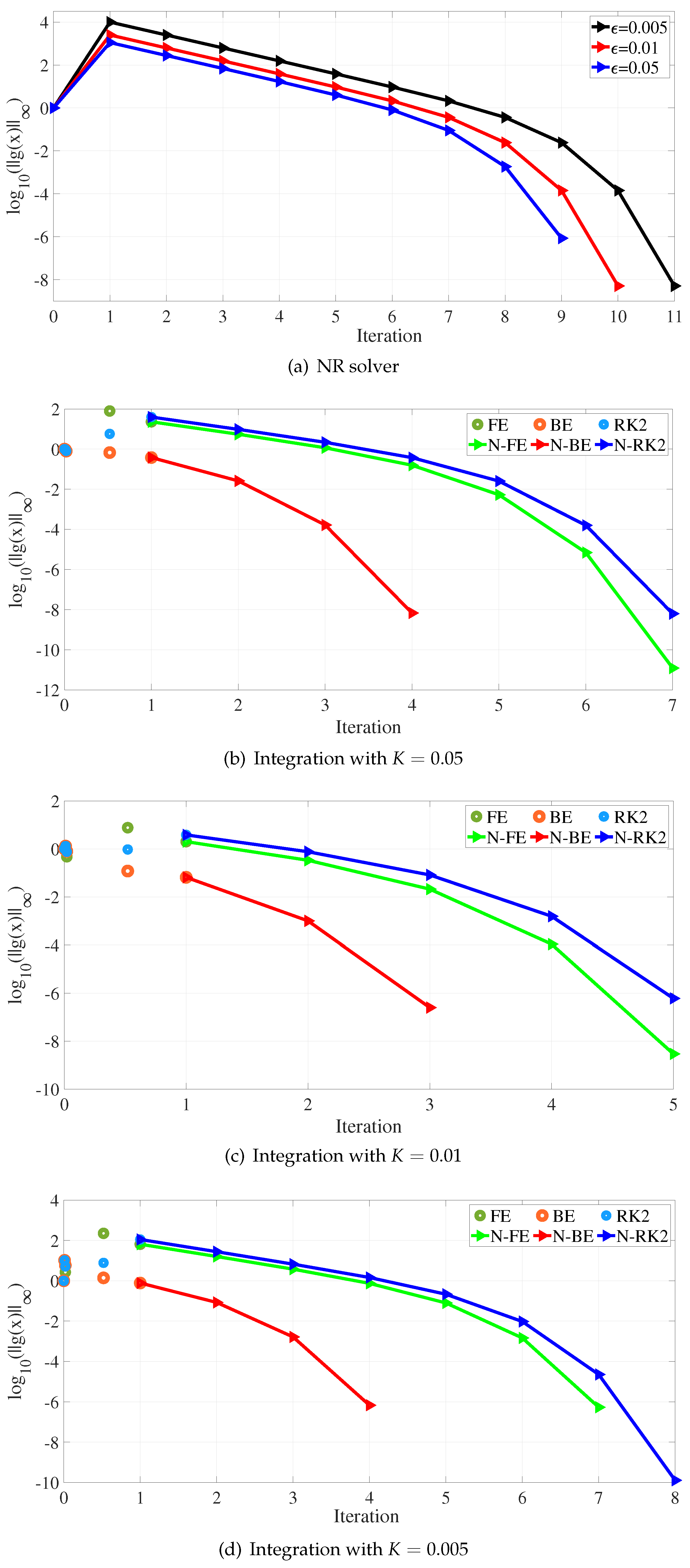
Figure 2.
Integration solver performance when a smaller step-length was adopted after the step .
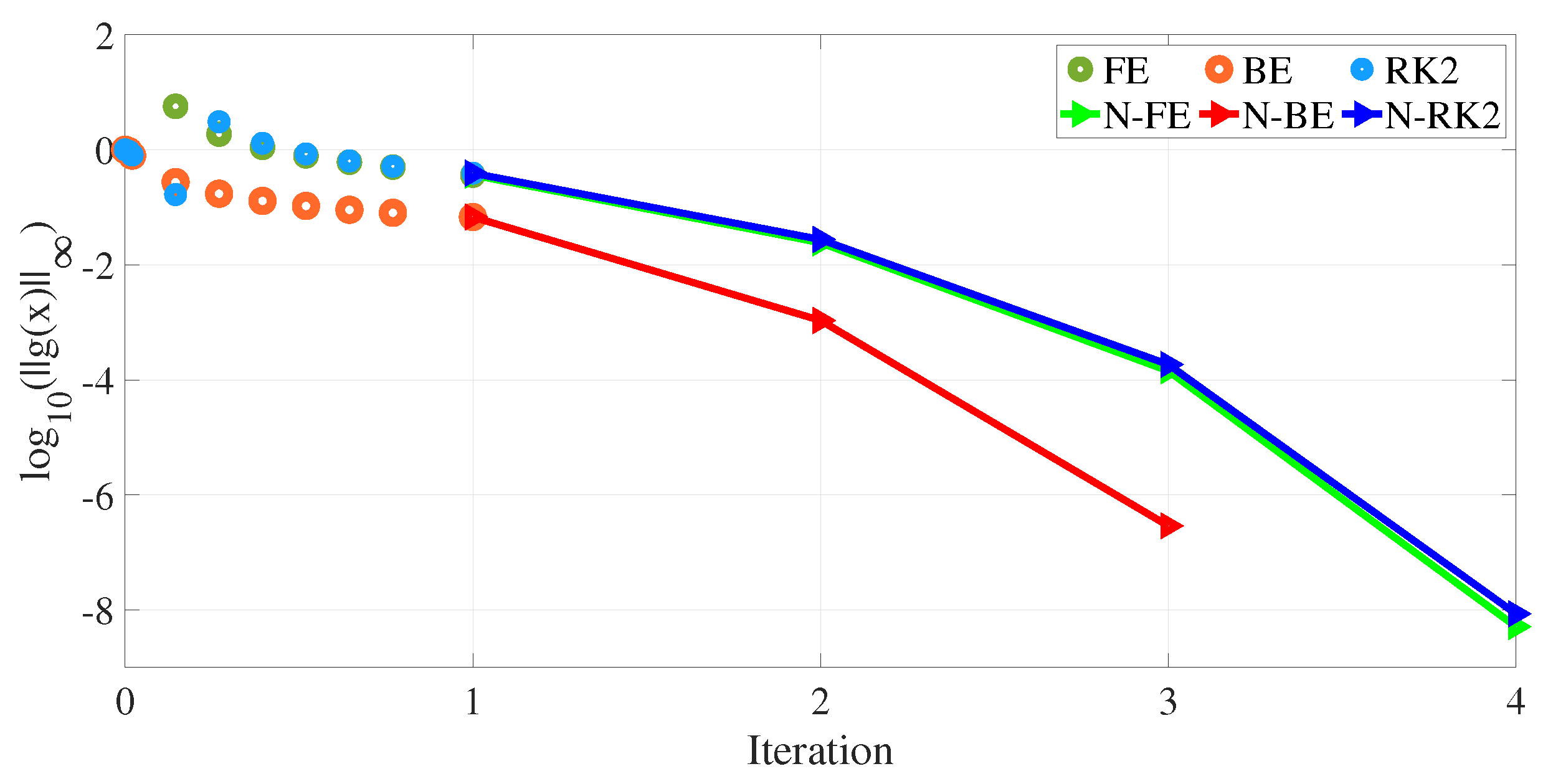
Figure 3.
Results for the evolution of states and decaying power mismatches for the case109272, when the BE solver is used for the dynamic homotopy process and the results are refined by the NR solver.
Figure 3.
Results for the evolution of states and decaying power mismatches for the case109272, when the BE solver is used for the dynamic homotopy process and the results are refined by the NR solver.
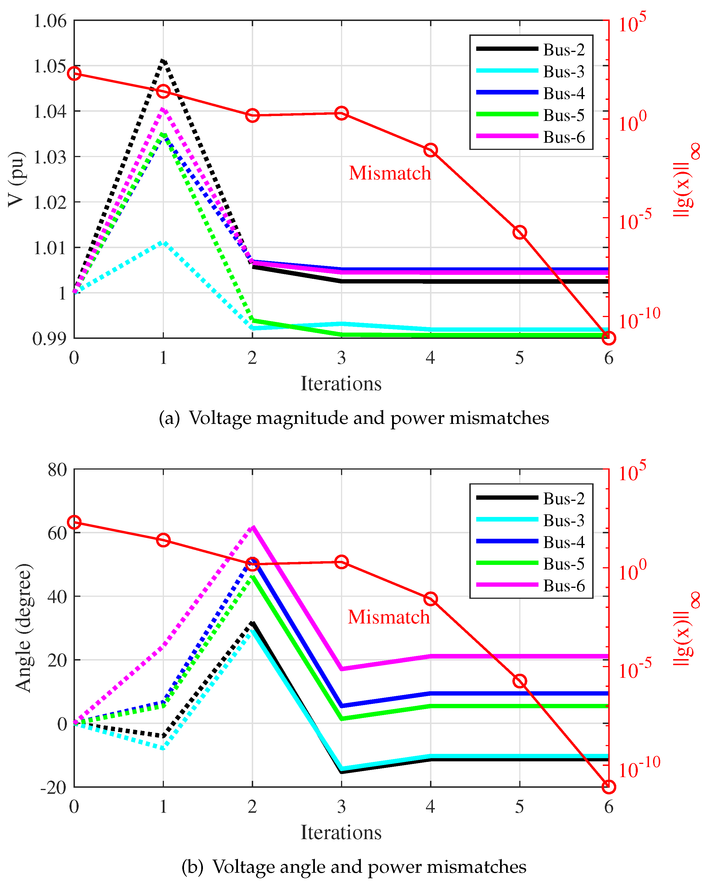
Figure 4.
Evolution of the voltage magnitude and phase angle with the index k of a time instant of the dynamic homotopy solver BE (dotted lines) or iterations for the NR solver (solid lines). Results are for the bus #6 of case109272, with different .
Figure 4.
Evolution of the voltage magnitude and phase angle with the index k of a time instant of the dynamic homotopy solver BE (dotted lines) or iterations for the NR solver (solid lines). Results are for the bus #6 of case109272, with different .
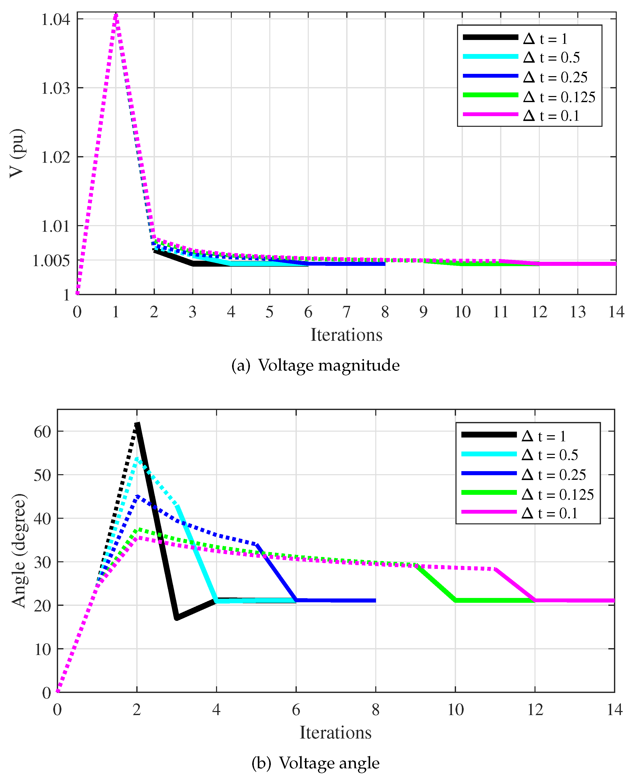

Table 1.
Ill-conditioned test systems according to new scenarios and originals [35].
Table 1.
Ill-conditioned test systems according to new scenarios and originals [35].
| Ill-conditioned case | Modified case | Number of buses |
|---|---|---|
| case18482.mat | case9241pegase× 2 | 18,482 |
| case27318.mat | case13659pegase× 2 | 27,318 |
| case36964.mat | case9241pegase× 4 | 36,964 |
| case54636.mat | case13659pegase× 4 | 54,636 |
| case109272.mat | case13659pegase× 8 | 109,272 |
Table 2.
Norm evolution for the FE solver combined with the NR solver for an initial time-step and large time-step for .
Table 2.
Norm evolution for the FE solver combined with the NR solver for an initial time-step and large time-step for .
| CASE/time | of the solver | NR | ||||||
|---|---|---|---|---|---|---|---|---|
| t or | 0.0 | 0.005 | 0.01 | 0.51 | 1.0 | 1 | 2 | 3 |
| case18482 | 532 | 65 | 9.7 | - | - | - | ||
| case27318 | 200 | 25 | 1.2 | 27 | - | - | - | |
| case36964 | 532 | 65 | 3.5 | - | - | - | ||
| case54636 | 200 | 25 | 1.2 | 27 | - | - | - | |
| case109272 | 200 | 25 | 1.2 | 27 | - | - | - | |
| case69limit | 0.012 | - | ||||||
| case141limit | 0.006 | - | ||||||
| case500limit | 13 | 1.2 | 0.02 | 0.9 | 1.0 | |||
| case2000limit | 54 | 3.9 | 0.8 | 210 | - | - | - | |
Table 3.
Norm evolution for the RK2 solver combined with the NR solver for an initial time-step and large time-step for .
Table 3.
Norm evolution for the RK2 solver combined with the NR solver for an initial time-step and large time-step for .
| CASE/time | of the solver | NR | ||||||
|---|---|---|---|---|---|---|---|---|
| t or | 0.0 | 0.005 | 0.01 | 0.51 | 1.0 | 1 | 2 | 3 |
| case18482 | 532 | 65 | 33 | - | - | - | ||
| case27318 | 200 | 25 | 13 | - | - | - | ||
| case36964 | 532 | 65 | 33 | - | - | - | ||
| case54636 | 200 | 25 | 13 | - | - | - | ||
| case109272 | 200 | 25 | 13 | - | - | - | ||
| case69limit | 0.012 | - | - | |||||
| case141limit | 0.006 | - | - | |||||
| case500limit | 13 | 1.2 | 0.6 | - | - | - | ||
| case2000limit | 54 | 3.9 | 1.9 | - | - | - | ||
Table 4.
Norm evolution for the BE solver combined with the NR solver for an initial time-step and large time-step for .
Table 4.
Norm evolution for the BE solver combined with the NR solver for an initial time-step and large time-step for .
| CASE/time | of the solver | NR | ||||||
|---|---|---|---|---|---|---|---|---|
| t or | 0.0 | 0.005 | 0.01 | 0.51 | 1.0 | 1 | 2 | 3 |
| case18482 | 532 | 65 | 33 | 7.2 | 3.7 | 0.04 | ||
| case27318 | 200 | 25 | 13 | 0.5 | 0.25 | 0.1 | ||
| case36964 | 532 | 65 | 33 | 6.9 | 3.6 | 0.27 | ||
| case54636 | 200 | 25 | 13 | 0.5 | 0.25 | 0.1 | ||
| case109272 | 200 | 25 | 13 | 0.5 | 0.25 | 0.1 | ||
| case69limit | 0.012 | - | - | |||||
| case141limit | 0.006 | - | - | |||||
| case500limit | 13 | 1.2 | 0.6 | 0.02 | - | |||
| case2000limit | 54 | 3.9 | 2 | 2.8 | 1.5 | 0.01 | ||
Table 5.
Evolution of norms with reduced initial time steps and progressive increments in computing the dynamic homotopy results, followed by three iterations of the NR solver.
Table 5.
Evolution of norms with reduced initial time steps and progressive increments in computing the dynamic homotopy results, followed by three iterations of the NR solver.
| CASE | solver/time | of the solver | for NR | ||||||||
|---|---|---|---|---|---|---|---|---|---|---|---|
| t or | 0.0 | 0.005 | 0.01 | 0.02 | 0.12 | 0.62 | 1.0 | 1 | 2 | 3 | |
| FE | 532 | 65 | 3.5 | 0.7 | 5.7 | 57 | 114 | 28 | 5 | 0.2 | |
| case36964 | RK2 | 532 | 65 | 33 | 16 | 9.6 | 4.2 | 2.6 | 0.2 | ||
| BE | 532 | 65 | 33 | 16 | 4.0 | 1.4 | 0.9 | 0.09 | |||
| FE | 200 | 25 | 1.2 | 0.02 | 0.07 | 0.3 | 0.17 | 0.03 | |||
| case109272 | RK2 | 200 | 25 | 13 | 6.3 | 1.2 | 0.5 | 0.3 | 0.19 | ||
| BE | 200 | 25 | 13 | 6.3 | 1.1 | 0.2 | 0.1 | 0.02 | |||
| FE | 55 | 3.9 | 0.8 | 0.7 | 3.6 | 58 | 91 | 16 | 1.0 | ||
| case2000limit | RK2 | 55 | 3.9 | 1.9 | 1.0 | 5.0 | 5.5 | 3.4 | 0.2 | ||
| BE | 55 | 3.9 | 1.9 | 1.0 | 1.0 | 0.3 | 0.2 | - | |||
Table 6.
Number of iterations (iterref) for the refining solvers (NR or FDXB) starting from partial results obtained by a dynamic homotopy solver for the experiments involving ill-conditioned and overloaded systems. Additionally, the iterations resulting from convergent actions of NR-MAT, NR-flat, and GSH-NR are shown.
| CASE | NR-MAT | NR-flat | GSH-NR | BE(NR) | RK2(NR) | BE(FDXB) | RK2(FDXB) | ||
|---|---|---|---|---|---|---|---|---|---|
| iter(NR) | iter(NR) | iter(NR) | iterref | iterref | iterref | iterref | |||
| case18482 | 6 | fail | 0.5 | 1 | 10 | 4 | 3 | 33 | 29 |
| case27318 | 5 | fail | 0.25 | 0.125 | 25 | 4 | 3 | 29 | 25 |
| case36964 | 6 | fail | 0.25 | 1 | 27 | 4 | 3 | 33 | 29 |
| case54636 | 5 | fail | 0.01 | 0.01 | fail | 4 | 3 | 29 | 25 |
| case109272 | 5 | fail | 0.01 | 0.01 | fail | 4 | 3 | 19 | 25 |
| case69limit | 4 | 4 | 1 | 1 | 4 | 1 | 1 | 8 | 8 |
| case141limit | 3 | 3 | 1 | 1 | 3 | 1 | 1 | 8 | 6 |
| ACTIVSg500limit | 3 | 4 | 1 | 1 | 4 | 2 | 2 | 13 | 11 |
| ACTIVSg2000limit | 3 | 5 | 1 | 1 | 5 | 3 | 3 | 22 | 20 |
Table 7.
Mean CPU Time in seconds for running experiments considering ill-conditioned test systems and solvers
Table 7.
Mean CPU Time in seconds for running experiments considering ill-conditioned test systems and solvers
| CASES | ||||||||||
|---|---|---|---|---|---|---|---|---|---|---|
| METHOD | case109272 | case54636 | case36964 | case27318 | case18482 | |||||
| NR-MAT | 3.8889 | (100%) | 2.1236 | (100%) | 1.8862 | (100%) | 0.8912 | (100%) | 0.8241 | (100%) |
| GSH-NR | fail | (-) | fail | (-) | 40.6900 | (2157%) | 21.5540 | (2418%) | 9.4790 | (1150%) |
| BE(NR) | 4.2730 | (110%) | 2.1840 | (103%) | 1.7260 | (92%) | 1.1430 | (128%) | 0.9040 | (110%) |
| RK2(NR) | 6.3920 | (164%) | 3.1070 | (146%) | 4.1100 | (218%) | 1.6240 | (182%) | 1.1630 | (141%) |
| BE(FDXB) | 2.6890 | (69%) | 1.4070 | (66%) | 1.0840 | (57%) | 0.7560 | (85%) | 0.6250 | (76%) |
| RK2(FDXB) | 4.1690 | (107%) | 2.0840 | (98%) | 1.5890 | (84%) | 1.0600 | (119%) | 0.9160 | (111%) |
Disclaimer/Publisher’s Note: The statements, opinions and data contained in all publications are solely those of the individual author(s) and contributor(s) and not of MDPI and/or the editor(s). MDPI and/or the editor(s) disclaim responsibility for any injury to people or property resulting from any ideas, methods, instructions or products referred to in the content. |
© 2024 by the authors. Licensee MDPI, Basel, Switzerland. This article is an open access article distributed under the terms and conditions of the Creative Commons Attribution (CC BY) license (http://creativecommons.org/licenses/by/4.0/).
Copyright: This open access article is published under a Creative Commons CC BY 4.0 license, which permit the free download, distribution, and reuse, provided that the author and preprint are cited in any reuse.


