Submitted:
02 January 2025
Posted:
06 January 2025
You are already at the latest version
Abstract
We define the function $Col: \mathbb{N} \to \mathbb{N}$ as the Collatz function, given by $3n + 1$ if $n$ is odd and $\displaystyle\frac{n}{2}$ if $n$ is even. The conjecture postulates that for any positive integer, at some point, its iteration will reach 1, or equivalently, every orbit will fall into the periodic cycle $\{4, 2, 1\}$. Two conditions would invalidate the conjecture: The existence of a divergent orbit or the presence of another cycle. We can study the dynamics of the orbits through the density of even terms in their orbit. If all points' accumulation density exceeds the value of $\displaystyle\frac{\ln(3)}{\ln(2)}$ then the orbit is bounded. The main result of this work is to show that there are no natural numbers such that the accumulation points of the pair density are less than $\displaystyle\frac{\ln(3)}{\ln(2)}$. In other words, there are no divergent orbits.
Keywords:
Collatz Conjecture
; Dynamical System
 |
 |
1. Background
A metric space is a set X equipped with a function , called a metric, that satisfies the following properties for all :
- Non-negativity: , and if and only if .
- Symmetry: .
- Triangle inequality: .
The function measures the “distance” between any two points x and y in the set X. The pair is called a metric space.
Examples of Metrics:
-
Euclidean Metric (on ):This metric defines the usual distance between two points and in Euclidean space .
-
Discrete Metric:In this metric, the distance between two distinct points is always 1, and the distance from any point to itself is 0.
-
Taxicab Metric (or Manhattan Metric, on ):This metric measures the distance between two points x and y as the sum of the absolute differences of their coordinates. It corresponds to the distance a taxi would drive on a grid of city streets.
-
p-adic Metric (on ):Here, p is a fixed prime number, and denotes the p-adic valuation of , whichThis metric measures the distance between two rational numbers based on their divisibility by p. The p-adic metric induces a non-Archimedean topology, meaning that the “triangle inequality” is strengthened to .
A complete metric space is a metric space in which every Cauchy sequence converges to a point within the space. Formally, a metric space is called complete if, for every sequence that is Cauchy (i.e., for any , there exists such that for all , ), there exists a point such that:
In other words, all Cauchy sequences in X must have a limit in X.
Examples:
- The Real Numbers with the Euclidean Metric: The set of real numbers with the usual Euclidean metric is a complete metric space. This is because every Cauchy sequence of real numbers converges to a real number.
- The Rational Numbers with the Euclidean Metric: The set of rational numbers with the Euclidean metric is not complete. For example, the sequence defined by and that approximate is Cauchy in but does not converge to a rational number (since ).
- The p-adic Numbers : The set of p-adic numbers , equipped with the p-adic metric , is a complete metric space. Every Cauchy sequence in converges to a p-adic number within .
Limit Superior (lim sup) and Limit Inferior (lim inf) of a Sequence:
Given a sequence of real numbers and . Let us consider the following subsequences of given by
we have that the sequence is monotonically increasing and is monotonically decreasing, that is:
Therefore there are limits
We will write and and we will call Limit Inferior and Limit Superior respectively.
Limit Superior (lim sup) and Limit Inferior (lim inf) of a Sequence of Sets: Let be a sequence of sets in a space X. The limit superior and limit inferior of the sequence of sets are defined as follows:
- Set Sequence limit superior ():
- Set Sequence limit inferior ():
-
Limit of a Sequence of Sets If , then the sequence converges, and its limit is denoted as:Particular Case: Monotone Sequences of Sets Non-Decreasing Sequence (): If is a non-decreasing sequence (i.e., for all n), then:In this case, the limit of the sequence is simply the union of all the sets in the sequence. Non-Increasing Sequence (): If is a non-increasing sequence (i.e., for all n), then:In this case, the limit of the sequence is simply the intersection of all the sets in the sequence.
A discrete dynamical system is a model of the evolution of a state over discrete time steps. Formally, it consists of a set X (called the state space) and a function that describes how the state evolves from one time step to the next. The system is described by the equation:
where represents the state of the system at the n-th time step. The evolution of the system is typically studied by iterating the function, f starting from an initial state . The sequence , where , is called the orbit or trajectory of the initial state .
Topologically Conjugate Dynamical Systems: Two discrete dynamical systems and are said to be topologically conjugate if there exists a homeomorphism such that the following diagram commutes:
In other words, the systems and are topologically conjugate if there is a bijective function such that:
 |
- h is a homeomorphism, meaning h is continuous, bijective, and its inverse is also continuous.
- The following relation holds:
This means that the dynamics of f on X and g on Y are the same up to a change of coordinates given by h. The systems and have the same qualitative behavior, such as the structure of orbits and periodic points, despite potentially differing in their specific representations.
Properties of Topological Conjugation with Respect to Orbits and Periodic Points:
- Preservation of Orbits: If and are two topologically conjugate dynamical systems, with a homeomorphism such that , then h preserves the orbits of points. Specifically, for any point , the orbit of x under f is mapped to the orbit of under g by h. Mathematically, this means:
-
Preservation of Periodic Points: If is a periodic point of f with period p, then is a periodic point of g with the same period p. Specifically, if , then:Conversely, if is a periodic point of g with period p, then is a periodic point of f with the same period p.
2. Collatz’s Conjecture
The Collatz conjecture, also known as the conjecture, is an unsolved problem in number theory proposed by the German mathematician Lothar Collatz in 1937. Despite its seemingly simple formulation, it has challenged mathematicians for decades due to the difficulty of proving its validity or finding a counterexample. The formal formulation of Collatz’s Conjecture is as follows:
Let , defined by:
then, for all exist such that:
An equivalent formulation of the conjecture argues that starting from any positive integer, one will eventually reach cycles . Two cases that could invalidate the Conjecture are that there is a cycle different from or that there is some divergent orbit. To date no evidence has been found for any of these options, however no demonstration has been presented that completely rules out these cases. In 2019 Terense Tao [15] presented a demonstration that almost every orbit falls in the cycle .
 |
Example 1.
Example 2.
2.1. Main Idea of This Work
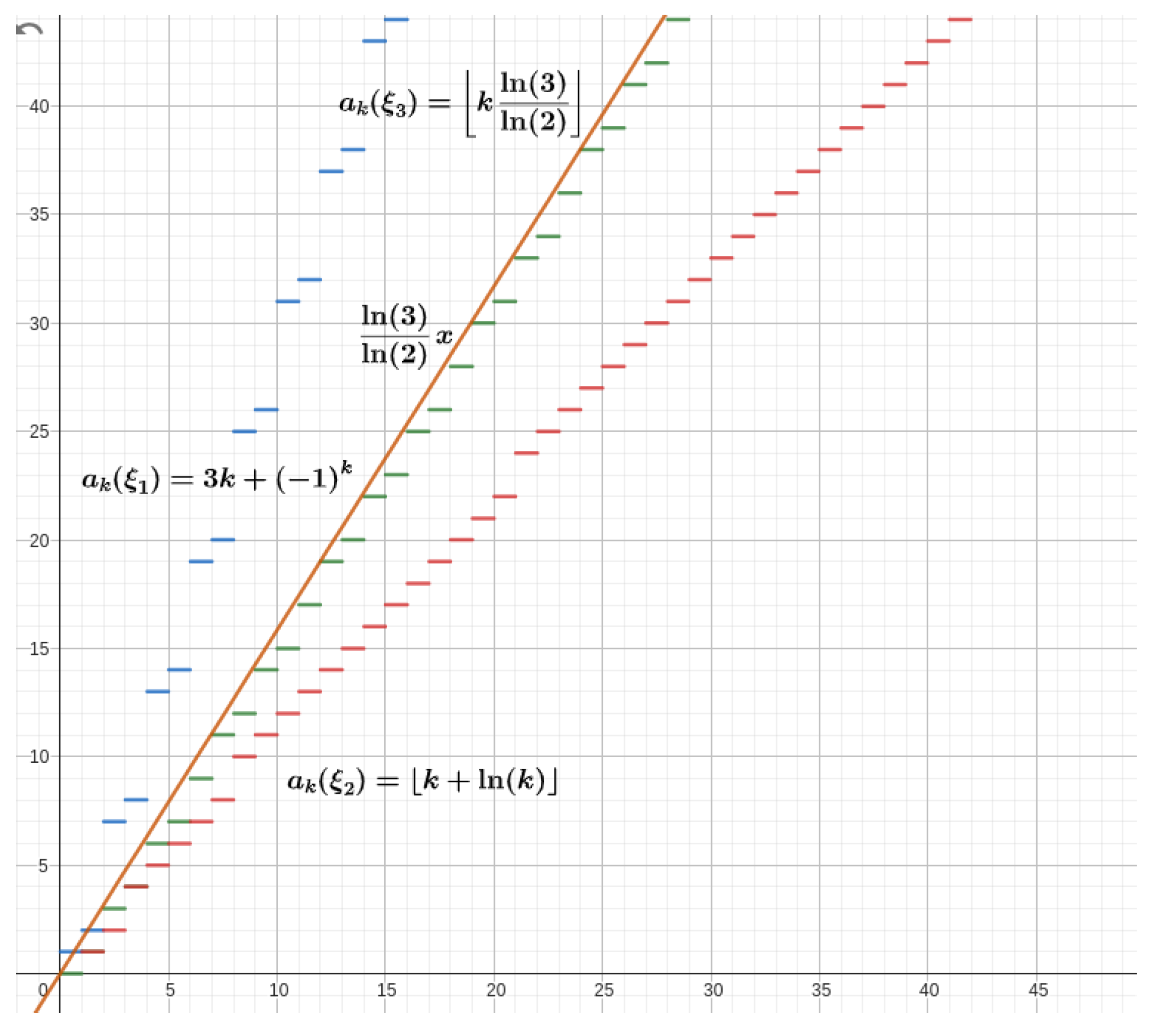
To each natural number, we can associate a unique binary sequence that represents the parity of iterations through the Collatz function. The sequence is defined as 0 if the number is even and 10 if the number is odd. We define the density function , where is the number of 0’s up to the k-th 1. These sequences can be classified into various sets depending on the behavior of the density function. However, we focus on three particular sets:
- : the set of sequences such that ,
- : the set of sequences such that ,
- : the set of sequences such that .
We have the following results on these sets
- (1)
- There is no such that its encoding belongs to .
- (2)
- If the coding of belongs to , then its orbit is bounded.
- (3)
- If is a periodic point, then its coding belongs to .
We will use these results to demonstrate the main result of this work Divergent Orbits Theorem:
Theorem 10:There are no divergent orbits for the Collatz function on natural numbers.
The idea of the proof is as follows: Suppose there exists an n whose orbit is divergent. Then necessarily, its encoding cannot belong to . This means there must exist a subsequence of the density function such that its limit is less than . Moreover, the density function of cannot have accumulation points greater than , because otherwise, there would exist a sub-orbit of n that is bounded. This is a consequence of the Corollary 7 where we obtain an upper bound for the sub-orbit of n. Since the set of possible values of the subsequence is finite, the subsequence must be periodic, causing the entire sequence to collapse into a periodic orbit. This would imply that the encoding belongs to , which would mean the orbit is bounded a contradiction. Thus, all accumulation points of the density function must be less than . In other words, . Hence, the encoding of n belongs to .
We now provide a brief demonstration of points 1, 2, and 3.
We use the following symbology to refer to an arbitrary composition of functions:
Let be real functions defined by
Define the set as:
We call k the length of S. This composition is unique for each element in (Proposition 3). Let we define the integer set of S as
This set is monotonically decreasing with respect to the composition of functions (Proposition 1). Let then
For any defines the minimum positive integer value of S
Let be a sequence of functions given by . Since the entire set is a mononally decreasing set with respect to the composition of functions in . We have that the minimum positive integer value is a monotonically increasing function, so
We will say that the sequence is positively stable if . Let with length k. We define the following application defined by
with
Theorem 8:Let with such that , then is positively unstable.
Now there is a relationship between the stability of the sequence and the existence of numbers with a given coding
Proposition 11:Let and of length k, then
Then suppose that there exists a natural number n whose coding is in and let be such that , then by Proposition 11 we have for all , exist such that for all , then is positively stable, which contradicts the Theorem 8. Therefore not exist such that . When we extend the Collatz function on rational numbers Definition 7 we have to given an coding , if there exists a rational whose coding is , then it is unique. On the other hand, by the Theorem 7, we have that if this rational exists, it must be negative. Therefore cannot exist such that its coding is in
Now we are going to show that there is no such that its coding is in . To prove this we are going to extend the Collatz function on the dyadic integers , initiated by Lagarias [9] (1985), defines (Definition 19) the following extension of the Collatz function on : Let be given by
It has been shown (see Mathews and Watts [10](1984) and Müller [11] (1991)) that the extended is surjective, not injective, infinitely many times differentiable, not analytic, measure-preserving with respect to the Haar measure, and strongly mixing. Similar results concerning iterates of may be found in Lagarias [9](1985), Müller [11] (1991), [12] (1994) and Terras [14] (1976). Defining the shift map as
Lagarias [9](1985) proved that is conjugate to via the parity vector map defined by
that is, . Bernstein [3](1994) gives an explicit formula for the inverse conjugacy , namely
See [6] page 57. In the notations that we will use in this work, we will denote the Bernstein function by and its inverse by . We will use instead of as the domain of the Bernstein function. As a consequence, we have that the periodic points of the Collatz function form a dense set. In particular, the periodic points of and are dense and admit rational representation Proposition 34. We will use these results to show that, in fact, the elements of are positive and negative unstable (Theorem 6). Then we have that there is no natural number whose encodings are in .
The second point we have:
Theorem 9:Let such that then the orbit of n is bounded.
In the Definition 20 the functions and defined on are introduced. Let be such that if the coding is in , then its orbit can be approximated through the function for relatively large values. In the Proposition 35, we have that when the coding is in then the function is upper bounded, then so is the orbit of n.
Finally in point 3, suppose that is a periodic point, then its coding is a periodic sequence in and by Proposition 11, we have that the sequence of functions on must be of the form for some , that is, n corresponds to the fixed point of . The fixed points are of the form , where this expression we obtain that the fixed point is positive in and negative in
2.2. Notations and Conventions
In this work, we are going to denote the set of positive integers as , the set of non-negative integers as and the greatest common divisor of a and b as and the least common multiple of a and b as .
We use the following symbology to refer to an arbitrary composition of functions:
3. Set Generate by and
In this section, we delve into functions generated by the composition of two real linear functions, and , focusing on their properties over integers. We define the set , representing compositions of these functions, and examine their orbits and associated sets of integers. Before delving into their properties, we introduce the crucial concept of the integer set of a function. Denoted as , this set represents the integers generated by the orbit of the function S. We emphasize the one-to-one correspondence between functions of the same length and the partition of integers into sets based on this length. These results provide a solid foundation for a detailed understanding of the properties of these functions and their application in the study of iterative functions over rational numbers.
3.1. Summary of Propositions in the Section
- Definition 1: Introduces the set , generated by two real linear functions and .
- Definition 2: Defines the integer set of a function as , where are functions in the composition of S.
- Definition 3: Defines the entire set of a function.
- Lemma 1 Monotony of Integer Set Lemma.
- Proposition 1: Establishes a relation of monotony in the entire sets concerning the composition of functions.
- Lemma 2 Establishes a characterization of the integer sets.
- Proposition 2: Establishes a one-to-one correspondence between functions of the same length and integer sets of the same length, and Affirms that the integer sets of functions of the same length are disjoint.
- Theorem 1: Ensures that the integer sets are the disjoint union of the integer sets of functions in with the same length.
- Proposition 3: Guarantees the existence of a unique sequence of elements for a function .
3.2. Set Generate by and
The Generated Spaces, denoted as . These spaces arise from the iterative composition of functions, where the individual contributions of and combine to form an enriched dynamic structure.
Definition 1
(Set Generated by and ). Let and defined by and , then we define the set as:
We will call the number n length of S.
Now let’s define the S-Orbits. These orbits are ordered sequences that reveal how each element evolves under the iterative action of the functions and .
Definition 2
(S-Orbit and Integer S-Orbit). Let and . We define the S-orbit of as the set:
Let . We will say that an S-orbit of p is integer when
Now let’s define The integer sets of a function, denoted by , represent the integer values that a specific function takes on its domain. Examining allows for the identification of patterns and regularities in the interaction of the function with integers, which is essential for understanding the structure of spaces generated by such functions.
Definition 3
(Integer Set of a Function). Let a function, we called integer set of f or the integers of f the set:
In the following Proposition we are going to see that integer sets have a monotonic behavior concerning the composition of linear functions, this property will be fundamental to studying integer S-orbits.
Lemma 1
(Monotony of Integer Set Lemma). Let such that and . Let and , then .
Proof.
In fact, we have Since there are solutions.
Let then by definition , then we have
as then we have
□
Proposition 1
(Monotony of Integer Set). Let with and . Then if we have:
Proof.
As the functions generated by are linear of the form with . The result follows inductively from Lemma 1. □
Example 3.
Let . We will calculate the integer set of
we have that and are solutions of the Diophantine Equation, then the integer set is:
Let then
indeed
The following lemma states that an orbit is integer if and only if its last value is an integer.
Lemma 2
(Containment in Integer Sets). Let , then if and only if with .
Proof.
Let then by proposition 1 we have with , then . On the other hand, we have then .
If with then so
then . □
In the following proposition, We will demonstrate that the integer sets associated with functions of the same length are disjoint. That is, if two integer sets share at least one element, then the functions must be the same.
Proposition 2
(One-to-One Correspondence and Disjointedness). Let of length k, if if and only if .
Proof.
Let and with and let be the largest index such that for all
If This means that they have different first terms. Then and or, and in either case we have .
Suppose that exist by proposition 1 we have
Taken
and by lemma 2
which is a contradiction, On the other hand if then otherwise we would have
however, neither set can be empty □
As a consequence of the above proposition we have
Theorem 1
(Partition of Integers). Let with length k, then
i.e., the sets of integers are equal to the disjoint union of the integer sets of functions S of length k
Proof.
it is evident that
To prove the other contention we consider the Collatz function defined by given by
let’s take an integer u and calculate its k-th orbit, this orbit can be written as compositions of functions in , let’s call the resulting function S since all the values of the orbit are integers, we have by the lemma 2 we can conclude that u is in the entire set of the function S.
□
So far we know that if two functions have the same length, then their integer sets are disjoint, this means that if we take elements of each integer set, the S-orbits of these integers are disjoint sets. Now, if we remove the condition that the lengths are the same, could it be that there is some number such that, given two different functions without being a part of another, it generates the same S-orbit? The answer is in the following proposition.
Proposition 3
(Uniqueness of Basis Representation). Let . Then there exists a unique sequence of k elements with such that
Proof.
Since , then there exists a sequence of elements with such that . Suppose for absurdity, that there is another sequence but of elements such that . Let , we have the following cases
-
If . We haveby Proposition 1 we have , since and then . Since and are invertible functions, we haveFollowing the same idea up to , we haveThe latter is impossible since the slope of the resulting line is of the form with . The case is completely analogous, therefore the case where and are different is not possible.
-
If . Since the sequences are different, there must exist some such thatthen by Proposition 2 we haveHowever, this is a contradiction to the Proposition 1, because for all . Then both sequences must be identical.
□
4. Stability and Instability of Integer Set
In this section, we delve into the stability and instability of sequences associated with integer sets. We begin by defining functions and that map real functions to integers. We introduce the concepts of positive and negative stability for sequences . The monotony of and is established through Proposition 1, demonstrating the non-decreasing of and the non-increasing of for a given sequence . Further, the Proposition formally defines positive and negative stability, incorporating limits and intersections of sets. The ensuing Stability Limit Theorem (2) establishes the asymptotic behavior of the integer set of an iterative sequence.
4.1. Summary of Propositions in the Section
- Definition 4: Definition of functions and .
- Proposition 4: monotony of the functions and .
- Definition 5: Definition of positively (negatively) stable (unstable) sequences.
- Theorem 2: Establishes the asymptotic behavior of the integer set when we have a positively (negatively) stable (unstable) sequence.
4.2. Stability and Instability of Integer Set
We initiate this section by introducing functions that associate each integer set with its minimum positive integer value and maximum negative integer value. These values are determined by the solutions closest to zero for the variable x in the Diophantine equation . This equation is representative of the Diophantine equation linked to an element within the space generated by and .
Definition 4
( and functions.). Define the function by
and
As a consequence of the Proposition 1. We have that the functions and are monotone.
Proposition 4
(monotony of and ). Let then is a non-decreasing function, and it is a non-increasing function.
Proof.
By the proposition 1 we have that
then and . □
From the result of the proposition above, we are going to make a classification of the sequences according to the behavior of the functions and .
Definition 5
(Stability of Sequences). Let sequence on given by . We will say that is positively stable if otherwise we will say that it is positively unstable. On the other hand, we will say that is negatively stable if , otherwise, we will say that it is negatively unstable.
Now we will give the central theorem of this section, which establishes the asymptotic behavior of the integer sets of from the stability or stability of this.
Theorem 2
(Stability Limit Theorem). Let and
and
We have:
- if is positively stable then
- if is positively unstable, then
analogously
- if is negatively stable then
- if is positively unstable, then
Proof.
: Let and with numbers from to and numbers from to . We have
supposed that is stable, we will first prove that is non-empty. By Proposition 1 the sequence of sets is a decreasing sequence of sets i.e. that the next set is a subset of the previous one, then the limit set corresponds to the intersection of all the sets of the sequence.
Now since is a function of the natural ones in the natural ones and is convergent, it implies that this function reaches its limit in a finite amount of steps
this implies
then the limit set is non-empty.
Now we will prove the limit set contains a single element. Suppose there exists another element that is contained in all positive integer sets, then there exists a non-negative integer t such that
without loss of generality, we can assume that is constant. Solving the equation in terms of t, we have
This solution is a fraction less than 1 for k large enough., which contradicts the fact that t is an integer.
Now let us take the unstable case. Suppose there exists an element in the limiting set i.e. an element that is contained in all non-negative integer sets, then there exists t a non-negative integer such that
as diverges and constant, then there exists a K such that is greater than , then cannot belong to any integer set with , which is a contradiction. Analogously for the other case. □
Example 4.
is positively and negatively unstable. Indeed, by example 3, we have where as then . On the other hand .
Example 5.
is positively unstable and negatively stable. Let’s calculate the integer set , let’s observe that
Then then we have and as
5. Coding of the Orbits
In this section, we will delve into the study of the coding of the orbits of the Collatz function. The main results of this section are the invariance of the coding between and on the fractions with denominator q and the one-to-one identification of each element of with its coding.
5.1. Summary of Propositions in the Section
- Definition 6: Coding maps and the space of sequences 0 and 10.
- Proposition 5: General form of the elements generated by and .
- Proposition 6: Fist Cod invariance: .
- Definition 9: Definition of .
- Definition 7: Extension of Collatz function on .
- Proposition 7: Extension of Collatz function on is well-defined.
- Proposition 8: .
- Definition 8: Extension of the Collatz function on .
- Proposition 9: equivalence: if then .
- Proposition 10: Second Cod invariance: .
- Proposition 11: if and only if
- Proposition 12 if and only if
- Proposition 13: .
- Definition 10: The Coding set .
- Proposition 14: Monotony of the Coding set .
- Proposition 15: Generating property: if then .
- Theorem 3: Uniqueness of the full coding .
5.2. Coding of the Orbits
It is a common practice in dynamical systems to encode orbits based on specific criteria. In our case, we will encode the orbits of the Collatz function according to the parity of its elements, assigning the value 1 when they are odd and 0 when they are even. Since our primary focus is on the Collatz function over , we will modify the initial coding by assigning 10 when it is odd, as opposed to just 1. We will denote the space where these codings reside as since it is a subset of the sequence space consisting of 0s and 1s, denoted in dynamics as . Formally, we express this as
Definition 6
(Coding of the Orbits). Let with length k. We define the following application defined by
with
To rigorously examine the properties of the coding, it is essential to establish a precise form for the elements generated by and .
Proposition 5
(General form of S). Let and Let and and let and defined as
then
Proof.
We will prove by induction on k. For we have
- , then, and then .
- , then, and then .
Suppose the statement is true up to k, let of length with H of length .
Claim 1: . We have:
- and for .
On the other hand, we have:
where we observe that the values coincide with those calculated.
Claim 2: . We have
- .
- .
On the other hand, we have
where we observe that the values coincide with those calculated, then the statement is true. □
Now we will see the first property of the coding
Proposition 6
(First Cod invariance). Let given by , we defined given by . Then .
Proof.
Let . To prove that they have the same coding, we have to prove that they have the same decomposition in principle, except that where there is we have a . let us observe that q has commutative properties with and .
- .
As then there exists such that
For convenience we will denote . Then we have
We have that if is then is still and if is then corresponds to . By Proposition 3 we have that the coding of has to be the same as that of S. □
Let us contemplate a generalization of the Collatz function applied to integers. In this variant, rather than adding 1, the function adds , where q is an odd integer. Subsequently, we will establish the compatibility of this generalization with the extension of the Collatz function to .
5.3. Extension of the Collatz Function on
As the concept of parity is a concept defined for integers, the Collatz function can be naturally extended to the set of integers. This concept is not trivially extended to the set of rational numbers, as there is no unique representation, We are going to consider a modification of extension on the rationals proposed by Lagaria in [9], Lagaria defined the Collatz function for fractions such that . We will distinguish two subsets of . The set of rationals with odd denominators, denoted by , and the set of rationals with even denominators such that the numerator and denominator are co-prime, denoted by . We will say that a rational number in is odd if the numerator is odd, and it is even if its numerator is even. In the case of , since the denominator is already even and due to coprimality, all elements are odd. We are going to consider the following extension of the Collatz function.
Definition 7
(Extension of the Collatz function). Let’s consider the following sets
and
We defined the Collatz’s function by by
We are going to show that the extension of the Collatz function that we defined is well-defined on
Proposition 7
(Well-Defined). The Collatz’s function on is well-defined.
Proof.
We are going to show that is well-defined over . Let with and . Let an odd number, then
□
Let’s observe that when we apply the Collatz function to with odd number, we always obtain a fraction with an even numerator, and when applied to , we always obtain an odd number. This will be very important since in Section 5, we are going to define how to coding the orbits, assigning 1 if it is odd and 0 if it is even, in the case of , we will have that all its elements have the same encoding which is unlike , where the codings will be generated by 10 and 0. For this reason we are going to work mainly on , let’s simplify the Collatz function a bit, as given by
Proposition 8
(Invariance of ). The Collatz function defined above satisfies that
Proof.
We will show that does not change the parity of the numerator.
-
if p is odd, we have with , thenSince q is odd, we have independent of the simplification .
-
if with , we haveSince q is odd, we have independent of the simplification, we have .
□
Considering the proposition above, we are going to define the Collatz function on as
Definition 8
(Extension of the Collatz function on ). We define the Collatz Function on by
Example 6.
Let and we have:
and
We can observe that the extension of the conjecture on the set of rationals is false, since we have found a fraction with a divergent otbit, The first objective of the work is to show that there are no divergent orbits in ..
We define the following generalization of the Collatz function.
Definition 9
(The map). Let , we define the Collatz function defined by given by
Now, we will demonstrate the compatibility of this generalization
Proposition 9
( equivalence). Let . Then for all integer numbers we have
Proof.
We let’s observe that
Suppose first that . This fraction is irreducible. Indeed, we have that . Then the parity of the fraction depends only on the numerator since there is no possibility of simplification that changes the parity of the numerator, and we can continue with the iteration for all k since the irreducibility of the iterations only depends on the initial fraction is irreducible. Then we have
Now to suppose that , for this case, the resulting fraction is not irreducible. However, as we are going to prove below, this does not change the parity of the orbits, so the formula would continue to be valid for this case. Suppose that, with and let . We will divide this proof into two parts.
Case one : We are going to prove the statement by induction. To
Now suppose that the statement is true for k, observe before continuing that the expressions and have the same parity. Indeed,
if the expression on the left-hand side is even, if and only if it is even. On the other hand, if the left side is odd, must be odd and if is odd, since the product of odd is odd, the left side is odd, so the expressions have the same parity.
-
if it is odd. Expanding the left-hand side of the proposition,developing the right-hand side of the proposition,We conclude in this case that both parts are equal
-
if it is even. Expanding the left-hand side of the proposition,developing the right-hand side of the proposition,We conclude in this case that both parts are equal. Since in both cases it gave equality, we conclude that the proposition is true.
Case two : We are going to prove the statement by induction. To
Now suppose that the statement is true for k, observe before continuing that the expressions and have the same parity. Indeed,
if the expression on the left-hand side is even, if and only if it is even. On the other hand, if the left side is odd, must be odd and if is odd since the product of odd is odd, the left side is odd, so the expressions have the same parity.
-
if it is odd. Expanding the left-hand side of the proposition,developing the right-hand side of the proposition,We conclude in this case that both parts are equal.
-
if it is even. Expanding the left-hand side of the proposition,developing the right-hand side of the proposition,We conclude in this case that both parts are equal. Since in both cases it gave equality, we conclude that the proposition is true.
□
We will define a coding function for the Collatz q-functions and demonstrate that they produce the same coding as the fractions with denominator q.
We are going to consider the set of sequences 0 and 10 that we will denote by and we formally define it as
this set can be seen as a subset of the set of sequences 0 and 1 where after the entry 1 enters 0. Let’s consider the following application: defined by
with
and
Proposition 10
(Second Cod invariance). Let an irreducible fraction with and defined by
with
then we have
Proof.
By proposition 9 we have
Since q it is odd, then, we have coding of and must be the same. □
We will now establish the initial connection between sets of integers and coding. Specifically, we will demonstrate that all elements within the integer set S share the same coding.
Proposition 11
(First characterization of ). Let and of length k with , then
Proof.
Let and then by definition by Proposition 1 we have with , then .
Suppose that then , then . □
We show below the second connection between the integer sets and the encoding. Specifically, we demonstrate that all values p within the integer set indeed have the same coding as the corresponding fraction .
Proposition 12
(second characterization of ). Let and of length k with , then we have: if and only if
Proof.
Let of length k such that , for the proposition 9, we have
then finally by the proposition 11, we have if and only if . □
The following proposition demonstrates that for a given rational number, we can generate a family of rationals that share the same encoding. This suggests that there exist many rationals with the same k-th encoding
Example 7.
Let’s consider the coding , we want to find rational numbers such that , we have that the function with coding ξ is
- , we have to calculate some solution of the entire set of . We have , then then .
- , we have to calculate some solution of the entire set of . We have , then then .
- , we have to calculate some solution of the entire set of . We have that , then then we have that .
Proposition 13
(Invariance property of Coding of rational). Let an irreducible fraction with , numbers from 0 to and then
.
Proof.
Let such that then this implies
then
□
As we have seen so far, we can characterize the entire set S from its encoding. Exploiting this property, we generalize the entire set S to encompass all fractions sharing the same encoding. We will call the Coding set.
Definition 10
(The Coding set). Let , we define the k-th coding set of
The encoding set also exhibits the property of monotony, similar to the integer set of S.
Proposition 14
(Monotony of the Coding set). Let then
Proof.
Let by definition then trivially we have , then . □
Definition 11
(The Coding set). Let , we define the k-th coding set of the coding set of
Similarly, the behavior of the solutions of Diophantine equations, in which knowing a particular solution allows us to determine other solutions, is reflected in the coding set. This connection is illustrated in the following proposition.
Proposition 15
(Generating property). Let , numbers from 0 to and then exist such that
Proof.
Let and such that , now consider and such that by proposition 12 we have the latter is equivalent
We are going to prove that and are elements of with . Indeed,
and
then
□
Now, we will present the main theorem of this section, establishing that the encoding of a rational number is unique.
Theorem 3
(Uniqueness of the full coding on ). Let . If it exists such that then it is unique.
Proof.
Let numbers from 0 to . Suppose there is another element, such than by proposition 15 exist such that
Since then for all . So
which is a contradiction. □
6. The Sigma Function
In this section, we immerse ourselves in the study of Diophantine equations of the form , where are integers. Solving these equations in the domain of integers x and y is a problem in number theory. Usually, these types of Diophantine equations are solved using Euclid’s algorithm or some similar technique, even by trial and error. However, these techniques begin to have a high degree of complexity for very large values. This mainly complicates when we want to study the behavior of the minimum positive values since in this case, we are interested in asymptotic solutions. We introduce the sigma function, symbolized as to address this challenge. This function, whose detailed analysis will constitute the core of our research, plays a fundamental role in the quest for specific solutions to the aforementioned Diophantine equations. Particularly noteworthy is the sigma function’s remarkable property of delivering solutions that are closest to zero in the context of these equations.
6.1. Summary of Propositions in the Section
- Definition 12: Definition of the sigma function.
- Theorem 4: Establish that and are solutions of the Diophantine equation . Additionally, is the minimum non-negative integer value.
- Corollary 1: Establishes that the minimum value grows based on the number of times the sigma function takes odd values.
- Corollary 2:
- Proposition 16: Establishes inequalities that estimate the values of the sigma function
- Proposition 17: It establishes the periods for the periodic points.
- Proposition 18: Establish algebraic properties of additivity, dependent on the parity of the addends
- Corollary 3 Establish algebraic properties’ linearity modulo
- Proposition 19 Establish that the sigma function is homogeneous modulo
- Definition 13: Extension of the sigma function on
- Definition 14: Characteristic Function
- Lemma 3: Establishes an invariance in the coding of the orbits of the sigma function.
- Proposition 21: Establishes homogeneity properties of the extension of the sigma function.
- Proposition 22 Algebraic properties of the Extension of the Sigma function.
- Definition 15: Definition of dyadic numbers.
- Proposition 23: Characterization of the dyadic representation of rational numbers.
- Definition 16: Definition of Cod-Sigma function.
- Lemma 4: Invariant coding lemma for Cod-Sigma function.
- Proposition 24: Change of basis of the Cod-Sigma function.
- Proposition 25: Let and and let such that and such that then
- Corollary 5: Let . Then .
- Proposition 26 is linear.
- Lemma 5: Rational equivalence of the Cod-Sigma function.
- Definition 17: we will say that has a null tail of index J if the smallest index such that we have .
- Proposition 27: and
- Lemma 6: .
- Proposition 28 .
6.2. The Sigma Function
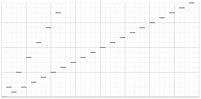
We are going to define the sigma function. This function is very similar to the Collatz function except that in this function, we do not multiply by 3.
Definition 12
(The Sigma function). Let such that . We define the sigma function
Figure 1.
Orbits of for .
In the following theorem, we explore solutions to the Diophantine equation , where a, k, and n are integers. This equation arises frequently in number theory, particularly in the study of Diophantine equations. We’ll demonstrate that the sigma function provides particular solutions for y, shedding light on the behavior of solutions in both positive and negative domains. Additionally, we’ll establish formulas for the smallest non-negative solution and the largest non-positive solution for the variable x, offering valuable insights into the structure of solutions to this equation.
Theorem 4
(Theorem on Diophantine Solutions). Let with and . Consider the Diophantine Equation . Then a particular solution for y is given by
where and . Furthermore. Let be the smallest non-negative solution for x, then
let be the largest non-positive solution for x if then
Proof.
We can write the sigma function as
Since the sigma function is defined on the set of integers in the integers, we have that its k-th composition is also an integer value: Let then
and Let then
replacing the k-th iteration sigma function in the equation and solving for , we have
and replacing the k-th iteration sigma function in the equation and solving for , we have
For the positive case, we have that , then due to the uniqueness of solutions in , L corresponds to the non-negative minimum value and for the negative case we have , again due to uniqueness of solutions in , we have that is the maximum non-positive solution. □
Example 8.
Let us consider the following Diophantine equation then
are solutions of the equation.
We will demonstrate that this minimum value increases every time is an odd number. This result is crucial for understanding how the parity of the sigma function influences the structure of non-negative solutions of the associated Diophantine equation.
Corollary 1
(Monotony relation). Let such that and and the minimum non-negative value of . Then increases every time is an odd number. In particular with if is even and if is odd.
Proof.
Let and then by Theorem 4 we have
then . So, we have that every time , the minimum positive integer value increases, and this only happens when is odd.
□
In the following corollary, we explore the relationship between the sigma functions and in the context of the Diophantine equation .
Corollary 2
(Relation between and ). Let and . Consider the Diophantine Equation, , then
Proof.
By definition, we have that is the nearest non-negative solution to 0, and is the nearest non-positive solution to 0, which means that and are consecutive solutions. Therefore, . then we have
Therefore □
In the following proposition, we examine the inequalities and estimations for the sigma function and , where n is an integer. We show that the sigma function lies in the interval for , and in the interval for . These inequalities are fundamental to understand the range of values the sigma function can take in the context of the considered Diophantine equations.
Proposition 16
(Inequality and estimation of the sigma function). Let and . Then,
Proof.
For we have two possible extreme paths, either we always get even or we always get odd, for the first case we would always have division by 2
for the second we would have
For , regardless of the cases, we always get a less stringent value to the initial value. If it is always even, we will have that it is always divided by 2, now in the case that it is always odd we have
and clearly, we have
□
6.3. Periodicity of the Sigma Function
Proposition 17
(Periodicity of periodic orbits). Let The sigma function has the following properties,
- The only fixed points are a and 0.
-
If, then, its orbit by is periodic with period given bywhere φ is the Euler’s totient function.In particular, if and then the periodic is . Let then
In particular, all points terminate in some periodic orbit (including periodic points) between 0 and a.
Proof.
we have
- Let , if u is odd, then which implies . If u is even, we have, which implies .
-
Let such that and , soThensuppose that , this implies that u is an invertible then, the equation is equivalentThe minimum value of k is given by the Carmichael function given byLet , thenas then , which is the necessary and sufficient condition for to admit decomposition in base 2 up to the power which implies that there exist such that .Now suppose that , then we divide by, dthen the development is completely analogous to the first case.In particular, when and u are co-prime with 3, then the period of the orbit of u corresponds to the Euler’s totient function, which in this case is .
□
Let us observe that for the equation to have a solution it is necessary and sufficient that since the function is monotonically decreasing for .
Example 9.
For, we have and .For we have , , and
6.4. Linearity of the Sigma Function Modulo A
In this section, we address the linearity of the sigma function modulo a. Proposition 18 establishes the addition rules for the sigma function under different parity conditions of the involved numbers. We will see in the corollary 3 that the function sigma modulo a is an automorphism of Furthermore, Proposition 19 establishing a relationship between and .
Proposition 18
(Algebraic properties of the Sigma function). Let and , then we have
- if are even numbers, then .
- if n is an even number and m is an odd number, then .
- if are odd numbers, then .
Proof.
Let , then we have
- If are even, we have
- If m is even and n is odd, we have
- If are odd, we have
□
This corollary states that the sigma function, seen as a function on the set and taking values in , acts as a group additive automorphism. In other words, it preserves the group structure under modular addition in
Corollary 3
(Linearity modulo a). We consider the function sigma as a function of in , then it is a group additive automorphism. i.e.
Proof.
From the previous proposition we have that the sigma function is linearly distributed except for a term that appears when both addends are odd, this term is congruent to □
This proposition establishes the concept of homogeneity modulo a for the sigma function. It relates the value of to under modular arithmetic. This relationship highlights a consistent behavior of the sigma function concerning scaling by m, providing valuable insights into its algebraic properties.
Proposition 19
(Homogeneity mod a). Let such that , then we have
Proof.
Let such that and consider the following Diophantine Equation . Since we have that, this equation is equivalent to . The Theorem 4 we have a particular solution of Y, then is a solution for y of , then
□
Proposition 20
(Fundamental equation). Let such that and , then
Proof.
Let n co-prime and less than . Let’s consider the following equation:
Let , then
Now we will prove that , we have
on the other hand
Let given we have
- and ,
- and if . That is to say that the function from this point on is monotonically increasing, therefore, from 2 we have that the function is always greater than 1.
then
Then we have for all n co-prime and less than , in particular we take
□
Corollary 4.
Let such that and , then
Proof.
By Proposition 17 and 20
□
6.5. Extension on the of the Sigma Function
We can extend the domain of the sigma function to the set of rationals, in the following way,
Definition 13
(-extension of the sigma function). Let . We define the sigma function
We are going to provide a numerical interpretation of the extension of the sigma function. Thus far, we understand that the sigma function provides us with the non-negative solution to the Diophantine equation through the equation . We can utilize the latter equation to extend the sigma function to the set of fractions with odd denominators, employing the following equation on :
or equivalently
That is to say, the extension of the sigma function gives the fraction that solves the equation
6.6. Properties of the Extension of the Sigma Function
The introduction of the sigma function extended to odd rationals is crucial for understanding its behavior in a broader domain. This extension, defined on the set , allows us to explore the algebraic and arithmetic properties of the sigma function in a more general context. In this section, we delve into this extension and explore its implications, focusing on how the sigma function modifies its behavior when applied to fractions with odd denominators. Additionally, we present an important lemma that establishes an invariant relationship between the characteristic function and the sigma function, providing a deeper understanding of how the sigma function preserves certain properties under different transformations.
Definition 14
(Characteristic Function). We define the characteristic function given by
The Invariant Coding Lemma, stated in Lemma 3, establishes a fundamental relationship between the characteristic function and the sigma function under certain conditions. Specifically, it asserts that for co-prime integers u and v, with u being odd, the characteristic function remains invariant under iterations of the sigma function. This means that the parity of the output of is the same as the parity of for all non-negative integers j. Furthermore, if v is odd, the lemma demonstrates that the parity of is identical to the parity of for all non-negative integers j.
Lemma 3
(Invariant Characteristic Function Lemma). Let with u not null, such that and then
- if v is odd then
Proof.
We have
-
Let where and where . We will prove by induction thatFor , Since if v is odd (or even) then is odd (or even) thenSuppose for , then , then we haveSince u is odd, we have that and have the same parity, then
-
Let where and where . We will prove by induction thatFor , Since v is oddSuppose for , then , then we haveSince v is odd, we have that and have the same parity, then
□
In the following proposition, we demonstrate homogeneity properties that leave the coding of the orbits of the sigma function invariant.
Proposition 21
(homogeneity). Let with u not null, such that and then we have
Proof.
We have
- Let where and where . Then we have
- Let where and where . Then we have
□
Proposition 22
( Algebraic properties of the Extension of the Sigma function ). Let with odd numerator and , satisfies the following identities
- (1)
- if are even fractions, then .
- (2)
- if is an even fraction and is an odd fraction, then .
- (3)
- if are odd fractions, then .
Proof.
Let’s proved first for . Let and let given by if n or m is even fraction and if n and m are odd fraction.
Dividing everything by , we have
Now let a an odd fraction with odd numerator, then we have is odd fraction, then multiplying by does not change the parity of or . Then we have
□
6.7. Coding of Sigma Function
6.7.1. The Adic Numbers
Kurt Hensel, a German mathematician from the late 1800s, is credited with creating the p-adic numbers. Their creation was in response to the requirement to expand the rational numbers in order to address algebraic and number theory issues that are difficult to resolve with just real numbers.
The notion of the p-adic valuation gives rise to the introduction of p-adic numbers, which offer an alternative to the standard metric based on absolute difference for measuring the “size” or “distance” between numbers. The largest power of p that divides n for a prime number p is the p-adic valuation of an integer n, represented by . The following formula extends this valuation to rational numbers:
where is a fraction of integers a and b, with . The associated p-adic metric is defined for any pair of rational numbers x and y as:
With regard to this metric, this metric offers a way to finish the set of rational numbers and produce the p-adic field . Every Cauchy sequence in can have a limit within thanks to the completion of with regard to the p-adic metric, completing the space and permitting a more flexible algebraic representation.
Every number can be uniquely described in terms of an infinite series consisting of positive powers of p and a finite number of negative powers in the p-adic field . In addition to generalizing the rational numbers, this algebraic structure offers strong tools for solving issues in number theory, algebra, and other mathematical fields.
Definition 15.
Let be any prime number. Define a norm on as follows
where
Let the completion of through the norm .
We have the following properties
- if then if and only if .
- Let then this is uniquely represented by convergent series ( with norm ) as
-
The adic expansion allows us to perform arithmetical operations in in way very similar to that in . Moreover, we will see that the operations in are, in fact, easier to perform than .Let and.
-
A adic number is said to be a adic integer if its canonical expansion contains only non-negative power of p. The set of adic integers is denoted by , soThis set has the property of being a complete metric subspace (Proposition 2.10 page 59 of [7]).
One of the main characteristics of adics numbers is
Proposition 23.
The canonical adic expansion represents a rational number if and only if is eventually periodic to the left.
6.7.2. Coding of Sigma Function
Now we are going to define the coding of the sigma function for .
Definition 16.
Let and odd number. We define the Coding of by σ as given by
and the finite coding as
The following lemma is a reformulation of lemma 3 for .
Lemma 4
(Invariant coding lemma). Let with u not null, such that and then
- if v is odd then
Proof.
Reformulation of the Lemma 3 □
Proposition 24
(Change of basis of the Cod-Sigma function). Let and with , and such that . Let given by . Then if and is an odd number we have
or if is an odd number we have
Additionally. if are odd numbers we have
Proof.
Let’s prove by induction that if is odd, then
Completing with if necessary, we have , then
Since we trivially have that and by hypothesis we have that , by the Lemma 1 we have
In particular, for , we have and is odd, we have then .
For , we have , then , then . Suppose this continues until for i.e.
We have that then by definitions and by inductive hypothesis then . Therefore, . Then we have to
Similarly, Completing with if necessary we have. Let , then
Now. If are odd numbers, we have
In particular, we have
then we have that the coding of is and of the is □
Example 10.
Let , we have , then
- , then . Then we have taking the coding coefficients, to base 2 we have
- , then . Then we have taking the coding coefficients, to base 2 we have
We observe that the obits are equal from the third iteration, which corresponds to the maximum power of two, where all subsequent coefficients are null. We can also observe that from the third term, the values that appear in the orbits are even, they, unfortunately, cannot continue forever, since as we have seen, the orbit of the sigma functions falls into a periodic orbit with the same number of even and odd numbers, so at some point this orbit must fall into an odd one, which means all the initial values must change.
Proposition 25.
Let and and let such that and such that then
Proof.
Let given by , then we want to find the minimum positive value of , then solving the following equation.
By Proposition 17 we have , then
Let such that . By Proposition 24 we have
□
Corollary 5.
Let . Then
Proof.
Let , and given by by Proposition 18 we have
Then
Let such that and and let such that
by Proposition 25 we have
Then we have
Then we have , therefore
□
Proposition 26.
Let . Then is linear:
Proof.
By Corollary 5 we have for all , this is equivalent to
Therefore
□
Example 11.
- 1.
-
Let , we have
- (a)
- then .
- (b)
- then .
then , Then we have - 2.
-
Let with even. We haveThen
- (a)
- then .
- (b)
- then.
Then we haveThen we have . - 3.
-
LetOn the other hand
- (a)
- then .
- (b)
- then .
Then we haveThenThat is, has a constant coding equal to 1. This is natural, since is stable.
Lemma 5
(Rational equivalence of the Cod-Sigma function.). Let , then we have
Furthermore. Let , then
Proof.
Let with . Let then multiplying by we have and subtracting, we have
On the other hand we have that , then
Other way for proof it, is
Now let’s demonstrate the second part. Let
On the other hand
Therefore □
Definition 17
(Null Tail). we will say that has a null tail of index J if the smallest index such that we have .
Proposition 27.
Let with and for and . We define . Let with null tail of index K given by with , for and for . We define if and if . We define the function given by and definite by if ξ is not null tail and if ξ has a null tail of index K Then we have and
Proof.
Without losing generality, let’s assume that does not have a null tail.
Claim 1: Let and , the we have .
Indeed. Let and . By Lemma 4, Proposition 26 and Lemma 5, we have
Since then .
Claim 2: .
Indeed. We have the following equivalence on (Proposition 3.3 page 76 of [7])
On the other hand
Therefore . On the other hand, we have that is a Cauchy sequence on . Indeed
and by Proposition 2.10 page 59 of [7], we also have that is a complete metric space, then . □
We will now show a connection between the minimum positive integer value and the encoding of the sigma function.
Lemma 6.
Let with . Then
Proof.
Let . Then
□
As a consequence of the next proposition, we have that if is a negative or non-integer number, the minimum value diverges, since we have that the dyadic representation of these numbers always has an infinite amount of numbers.
Proposition 28.
Let and . Then , where is the quantity of 0 of
Proof.
Let us assume without loss of generality that is not null tail.Let . So
Then □
7. The , and sets
Let . Let the quantity of 1 of . Define the function . This function corresponds to the slope of the function such that . Let us consider three subsets that will be relevant to study the non-existence of divergent orbits. and which correspond to the subset of the sequences such that converges to 0, ∞ and some real respectively.
7.1. Summary of Propositions in the Section
- Definition 18: Sets , and .
- Lemma 7: Characterization of and through accumulation points of .
- Proposition 29: Let then exists such that .
- Lemma 8: Let , then satisfies the following inequalities and if .
- Proposition 30: Let , then is not convergent.
7.2. The , and sets
We can consider the following set of :
Definition 18
(The , and sets). Let with and for or with , for and for . Let . We will consider the following subsets of
and
Example 12.
- Let such that , then .
- such that , then
- Let such that , then
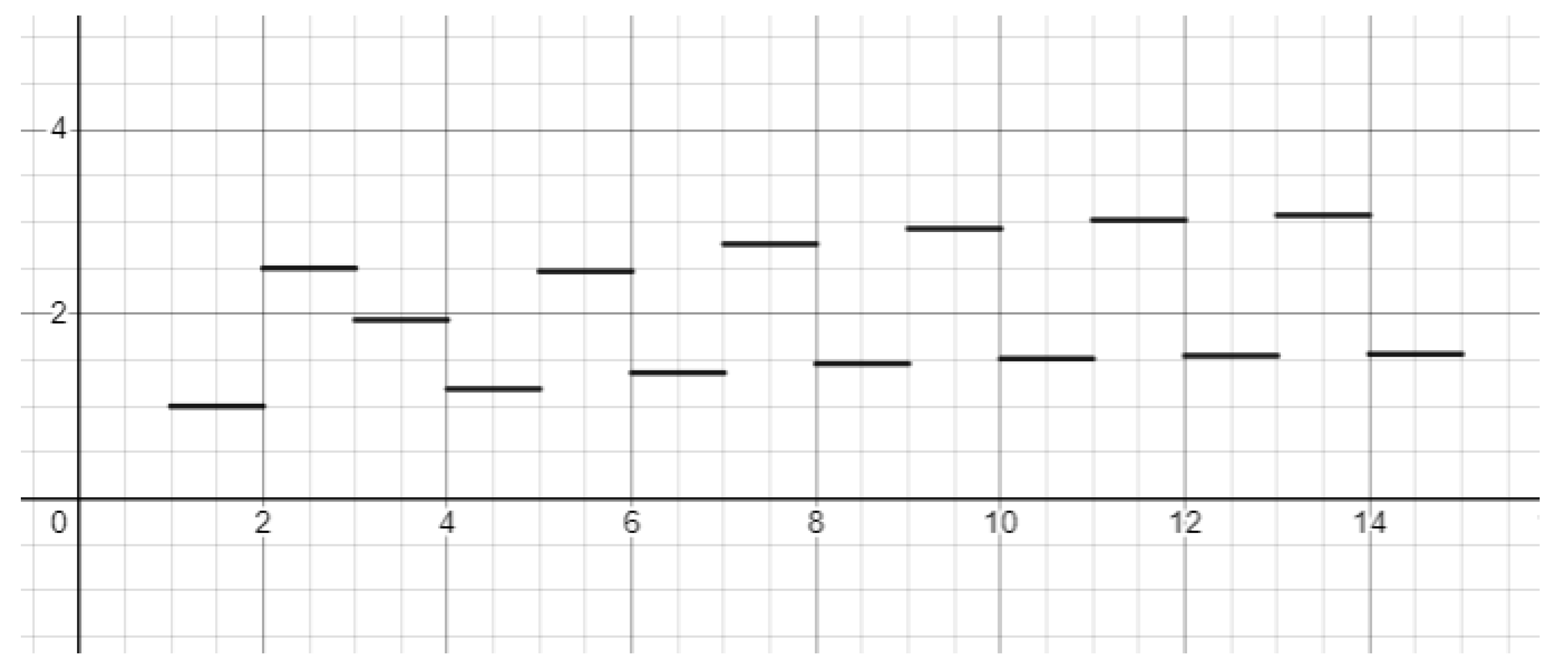
Figure 2.
The sequences in have their counting function 0 above the graph of the function , the sequences in have their counting function 0 below the graph of and the sequences in have their counting function 0 tending to the graph of the function .
Figure 2.
The sequences in have their counting function 0 above the graph of the function , the sequences in have their counting function 0 below the graph of and the sequences in have their counting function 0 tending to the graph of the function .
The following result establishes a characterization of the elements of and . We begin by providing a technical definition that we will use for the subsequent results.
Lemma 7.
Let such that ξ is not null tail, then
- if and only if as .
- if and only if as .
Proof.
-
Let’s suppose that as and suppose that . Then let , then exist such that for , then we have,which is a contradiction.Now, let then . Then exist such that for all . Then
-
Let’s suppose that as and . Let , then exist such that for , then we have,which is a contradiction.Now, Let then , Then exist such that for all . Then
□
Now we will show what happens when .
Proposition 29.
Let then exists such that on .
Proof.
Let , then . Let’s prove that exists such that . If there exists a subsequence such that as then which contradicts the fact that . On the other hand if there exists a subsequence such that as then which contradicts the fact that , then exists such that . □
Lemma 8.
Let , then ε satisfies the following inequalities and if .
Proof.
Let us verify that satisfying satisfies both inequalities.
- For the first inequality: , expanding and simplifying, we have Since is less than , this inequality is satisfied.
-
For the second inequality: First we will prove the following inequalityfor , indeedthis inequality is also satisfied.Now thenSince is less than and .
□
Proposition 30.
Let , then is not convergent on .
Proof.
Suppose that and exist such that . Let then exist such that . On the other hand we have , so
By Lemma 8 we have
- if , then . Therefore
- if . then . Therefore
Therefore is not convergent. □
8. The Extension of Collatz Function on
In this section we will study the extension of the Collatz function on proposed by Lagaria in [9], and in an analogous way we will define the dyadic integer sets and the encoding set. We will prove that given an coding there exists a unique dyadic integer with this coding. We will show that this extension is topologically conjugate to the shift function in and we will use this result to prove that codings in are unstable.
8.1. Summary of Propositions in the Section
- Lemma 9: Equivalence of the parity of fractions and their dyadic representation.
- Definition 19: Extension of the Collatz function on the set of dyadic numbers and the definitions of dyadic integer set and coding set.
- Proposition 31: Characterization of the dyadic integer set.
- Proposition 32: Establishes that the Coding set and the Dyadic Integer Set are the same.
- Proposition 33: It establishes that given a coding there is a unique dyadic number with said coding.
- Theorem 5: The Collatz function on the set of dyadic numbers is topologically conjugate to the Shift function.
- Corollary 6: The periodic points of the Collatz function in are dense in .
- Proposition 34: The periodic sequences of correspond to positive periodic points of the Collatz functions and the periodic sequences of correspond to negative periodic points of the Collatz functions.
8.2. Extension of the Collatz Function on
Now we are going to extend the Collatz function to the set of . In order for the extension to be compatible with the results obtained in the previous sections, we will first show that the parity of the elements of is preserved in .
Lemma 9.
Let the dyadic representation of , then p is even if and only if and p is odd if and only if .
Proof.
Let p a even number, so we have
Let p a odd number, so we have
□
Now let us consider the following extension of the Collatz function on .
Definition 19.
Let given by
with if and if . Let then we defined the Coding set of ξ
Let , we define the dyadic integer set of S as
Next we will show the version in to the results seen in previous Sections. The following Proposition characterizes the set of dyadic integers of analogously to the entire set.
Proposition 31.
Let and such that . Let , then .
Proof.
Let then we have . Indeed. Let and such that , then
so
Now . Let , so , so
Therefore, we have
□
The following proposition states that the entire dyadic set is equal to the coding set of .
Proposition 32.
Let and such that . Then
Proof.
Let , so by definition we have . We can rewrite as for any and . We Claim that . Indeed
We have that the parity on the right side only depends on , then the latter must have the same coding as by Proposition 11 we have . So , so .
Let and let , then . On the other hand, since trivially has a representation as a natural number, we have that it is also a natural number, so by Proposition 11 we have that . By hypothesis we have that , then exist such that , applying times with , we have
Since is always even for all , we have that the parity of each iteration only depends on , then . □
In theorem 3 we saw that given if there exists a rational whose encoding is exactly , then it is the only rational solution. However we could not guarantee the existence of such a number. The following Proposition guarantees us that there exists a solution in the set of dyadic numbers.
Proposition 33.
Let , then exist an unique such that
Proof.
Let by Lemma 27 we have . Now we are going to prove that:
Claim for all . Indeed, let such that then , we have for all , Then
By Proposition 32 we have for all . Since , we have
Suppose there exists another dyadic integer such that it is also in , then
Therefore . □
The existence of solutions to the equation in the dyadic numbers does not guarantee the existence of rational solutions. This will depend primarily on whether the dyadic solution can be represented as a rational number or, more generally, as a real number. Based on the nature of this solution, we can determine whether or not a rational solution exists.
8.3. Topological Conjugation
The Shift function on is defined as the mapping that deletes the first term of the sequence. The following theorem states that the Collatz function on is dynamically equivalent to the Shift function on and that the function is a homeomorphism between these two spaces. A similar result can be found in [9] where the Shift function is defined on instead of .
Theorem 5
and is a homemorphism.
( is topologically conjugate to ). Let given by
is topologically conjugate to ω i.e the following diagram is commutative
 |
Proof.
Let’s first prove that the diagram is commutative.
Let with . Writing this way, we get an explicit form for the function . If we have
and
where both parts are equal. On the other hand. suppose that with and . We have
and
where again both parts are equal. Then we conclude that the diagram is commutative.
Now we are going to prove that is a bijection.
Let given by if and if . Let’s prove that and
- : By Corollary 33 we have .
- : Let and such that , so for all . On the other hand we have for all . Let the number of 0 of Exists for all such that so then as Thus .
Let us show that the applications and are uniformly continuous. Let the symbolic metric of two symbols given by
and
The space is a complete metric space with the property that if two sequences are arbitrarily close if and only if their first terms are equal.
is uniformly continuous: Let and such that and . So let
Let the number from 1 to the -th term of , then for ,
so , then in particular
so
is uniformly continuous: Let and such that and such that then , so , so .
Therefore is a homemorphism and is topologically conjugate to . □
8.4. Periodic Point
As a first consequence of topological conjugation, we have that the set of periodic points of the Collatz function is dense in .
Corollary 6.
Let the set of periodic point of ω, then we have
Proof.
consequence of the continuity of the function and the fact that the periodic sequences of the Shift function are dense in . □
As a consequence of the topological conjugation we have that is a periodic point if is periodic, we are going to show that the periodic points in are positive and the periodic points in are negative.
Proposition 34.
Let periodic and , then we have:
- If so has positive rational representation.
- If so has negative rational representation.
Proof.
Let with . Considering that so we have , Let us first show that with for all :
We are going to show that is rational
which corresponds to a rational number. For the case with , we take , we have that even is of period, then
then
where its sign depends on the denominator , if are in if and only if as if and only if so the denominator is negative, so is positive, analogously when is in if and only if as if and only if so the denominator is positive, so is negative. □
9. Real Function and Function
Let’s define a new function defined on given by , unlike case does not have a null tail and when it has a null tail with index J. It is not always convergent. Does this mean that when it is divergent, then there is no solution to the encoding problem? The answer is no, for example if we take the encoding which corresponds to the encoding of 1, however the function is divergent. As we will show in the next section, when it is convergent, it is in fact the only solution to the encoding problem. In addition to the real function , we will define the function which unlike which is a series, this is a function on the natural numbers to the rational numbers. We will show that the function is convergent if and only if and that the function is bounded if and only if .
9.1. Summary of Propositions in the Section
- Definition 20: We will give the definition of the functions and .
-
Proposition 35 Characterization of and through functions and .
- (a)
- if and only if .
- (b)
- if and only if is bounded.
- Lemma 10: Let . Then exist such that if we have
- Lemma 11: Let , if then, we have .
- Corollary 7: Let . If exist a sub-sequence such that . Then exist such that .
- Definition 21: Definition fix function.
-
Proposition 36: Let and and . Then we have:
- (a)
- if then exist and .
- (b)
- if then is bounded and if is a subsequence convergent then .
- (c)
- if then
- Theorem 6: Let , then not exist such that . In particular is positive and negative unstable.
9.2. The and Functions
We will give the definition of the functions .
Definition 20
(The and functions). Let without null tail given by with and for . Let . Define the function given by
and defined by
and defined the function as
and by
Let with null tail and index given by with and for . Define
and by
Example 13.
We will give some examples of the functions and :
- 1.
-
Let
- (a)
- .
- (b)
- for and
- 2.
-
Let then we have
- (a)
- (b)
- 3.
-
Let then we have
- (a)
- .
- (b)
- 4.
-
Let
- (a)
- . Since, .
- (b)
- 5.
-
Let then we have
- (a)
- .
- (b)
-
,,and
Figure 3.
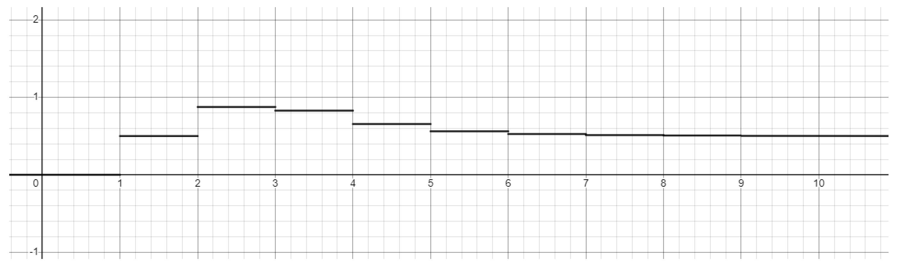
Figure 4.
The following result establishes a characterization of the elements of and for the behaviour of the functions .
Proposition 35
(Characterization of the and sets). Let and . Then
- if and only if .
- if and only if is bounded.
Proof.
Proof of the first statement. Is obvious for the case of null tails with index J, since we have it is automatically finite, and as we see in the examples would be of the form when which implies that is finite.
So we are going to assume that has no tail null.
Suppose that , then by Lemma 7 we have , so, there exists such that for all we have that
Let’s suppose , then
so then
□ of the first statement.
Proof of the second statement
. Suppose is bounded, we will prove that converges to 0. Suppose for for any . Then we have
We have that the sum on the right is divergent.
which generates a contradiction to the fact that is bounded.
To demonstrate the other implication, let us consider the following lemmas:
Lemma 10.
Let . Then exist such that if we have
Proof. Let and , then we have
On the other hand, by definition of lower limit, we have
Then exist such that if we have
□
Lemma 11.Let , if then, we have .
Proof. Let writing explicitly, we have with and for , then we can write:
Suppose . Since the minimum value that can take is 1, we have
□
By Claim 3 and 4 we have, exist such that if we have
Then by claim 5, Let so
Let . Then we have . Then we conclude that is bounded.
□ of the second statement.
The following result is the version of the previous theorem for sub-sequence.
Corollary 7.
Let . If exist a sub-sequence such that . Then exist such that .
Proof.
Let then
then exist such that if we have
Using the lemma 11 we have
Therefore □
9.3. The Set Is Unstable
Definition 21.
Let without null tail, define the fix function as given by
This functions associates to each sequence the fixed point associated with the function such that . Next we will see the behavior of the function when is in and .
Proposition 36.
Let and and . Then we have:
- if then exist and .
- if then is bounded and if is a subsequence convergent then .
- if then there exists a positive monotonic and divergent sequence such that
Proof.
Let , then:
- If and let by Proposition we havethen
-
If then . On the other hand, we have the following.Then if is a convergent subsequence, then . Now we will demonstrate that is bounded. Let such that then
-
If , then exist such thatSuppose that exist a sequence such that as , this is equivalent to as soThis contradicts Proposition 29 where it states that there exist such that for all .Therefore, we haveLet us denote by , as , then we have that is monotonically increasing, on the other hand as , then by Proposition 35 we have that as
□
Theorem 6.
Let , then not exist such that . In particular ξ is positive and negative unstable.
Proof.
Let , for simplicity we will assume that . Let’s assume that it is stable, that is, it exists such that and let then we have
Let be a periodic sequence of period such that the first terms of coincide with the first terms of . For example:
Due to periodicity, we have . By Proposition 34 we admit a rational representation
By the continuity of the function we have that as on . On the other hand. By Proposition 36 we have
where is a monotonic and divergent sequence real. This means that the sequence is unbounded in . Due to the uniqueness of the limit we have to , this is a contradiction to assumption that is stable, we have that is unstable. □
10. The Coding of
Now we are going to prove that there is a complete metric on . We will use this result to prove that if then and in the case that , then there is no rational r such that . We also show that the parity of the Collatz function on depends solely on the first term. Building upon this insight, we extend the Collatz function to and conclude the section by showing that the Collatz function is topologically conjugate to the Shift function in . We will use this result to establish that the set of periodic orbits is dense.
10.1. Summary of Propositions in the Section
-
Lemma 12: Established that when the functionthen and share at least the first terms.
- Proposition 37: Establishes that is a complete metric space.
- Corollary 8: Established that the coding set is an open set.
- Theorem 7: Established that the full coding set is a singleton set or an empty set depending on whether is rational or not.
- Proposition 38: is continuous.
- Corollaty 9: The is a continuous function with the usual metric of
- Proposition 39: It establishes that the parity of depends only on the first term of the series.
- Definition 22: Defines an extension of the Collatz function on all .
- Proposition 40: The Collatz functions are continuous.
- Proposition 41: The Collatz function on is topological conjugacy to Shift map on
- Corollary 10: It is stable that the periodic points of the Collatz function in are dense.
10.2. as Complete Metric Space
To ensure the coherent definition of a metric in , we need to “complete” the missing terms of the series to enable the calculation of the difference for all , irrespective of whether or has a null tail. To accomplish this, we define that when the sequence of 1s in ends, the function will take on the value . Hence, we have from the index of . Let with null tail with index J. We will write a short description.
In the following lemma, we are going to introduce a new function, which, as we will see later, corresponds to a metric in the space . Additionally, we will present another result that we will examine more closely in this section and essentially indicates to us that, since the parity of depends only on the first term, we can interpret this in the following way: If two sequences are arbitrarily close, then they share the first terms of their encoding. This is of great importance for understanding the behavior of the orbits of the Collatz function, since, if we consider the Euclidean metric in or that of the absolute value, we observe the phenomenon that even though two numbers are arbitrarily close, their dynamics are completely different. One may converge to a cycle in a few iterations, while the other may take a very long time.
Lemma 12
(Convergence and Coincidence Lemma). Let , then
- is well defined.
- . In addition, we have to for all .
Proof.
Let , then we have
Claim Let, then . If , then . Suppose that then
□ of the Claim.
Now we prove that it is well-defined, by Claim we have:
as and converge to 0, then for exist such that if we have
Then for we also have
Then we have that also converges to 0. Then by Proposition 35 we have . To prove the statement, we will consider whether the sequences and in have a null tail or not.
Let us first assume that the sequence does not have a null tail, then if we have
All terms less than r must be null. Suppose there exists some non-zero term between 1 and , then we have that
which is absurd. Then we have that . Which implies that
Now we will prove that the sequences coincide up to r.
writing this way, we have to
then
which means that and share the first blocks Now suppose that has a null tail of index and has no tail null. Then we have
if then we have the previous case, then . Now if we have
The latter makes sense if also has a null tail of index , then
In particular . Finally, suppose that and have a null tail of index and respectively, without loss of generality we can assume that . Then
- If then all terms with an index less than r are null and in particular we have for . and as we already saw in the proofs above, this implies that for all .
- If . Then we have that therefore . particular we have for .
□
Now we are going to show that the function we defined above is a complete metric on
Proposition 37
(Metric space complete). Let given by
Then is a metric space complete.
Proof.
Let’s prove that d is a metric through the axioms of metric:
-
if and only if for all : Trivially we have that if , thenLet such thatby lemma 12 we haveIn particular, for we have .
- for all :then
- for all,then
then is a metric space. Now we are going to prove that it is a complete metric space. Let be a Cauchy sequence on then for any exist such that
Let such that by lemma 12 we have
On the other hand let the symbolic metric of two symbols given by
with
The space is a complete metric space with the property that if two sequences are arbitrarily close if and only if their first terms are equal.
then given a Cauchy sequence in by the observation above we obtain a Cauchy sequence in and the latter being complete there is a such that
We will now prove that is in and that the sequence converges to .
-
Let’s prove that is complete. Let a Cauchy sequence on and let . Let’s show that . Let , then by definition we have exist such that for all , so we have and have the first R terms equal, Suppose has no null tail, then thenIf has a null tail, then by definition it is in .
-
Let’s prove that is complete. Let a Cauchy sequence in . Let , then exist N such thatby Lemma 12 we have for all . In other words we have that is a Cauchy sequence in . As we proved in point 1, we have that is a complete metric subspace of , so exist such that . Let us now demonstrate thatTherefore it is a complete space.
then we can conclude that the metric space is complete. □
With this metric, we have that the coding sets are open sets.
Corollary 8
( is an open set). Let and . Then is an open set on
Proof.
Let and such that . Let us consider v in such that , by definition, exist such that and . By Lemma 12 have for , then we have that . Therefore, then i.e. the ball of radius and center u is a subset of , therefore is an open set. □
Proposition 38.
is continuous.
Proof.
Let and a sequence on such that , so for all , then we have
Therefore as , that is to say that es □
Corollary 9.
The is a continuous function with the usual metric of
Proof.Let a sequence on such that . By continuity of we have
□
10.3. Characterization of the Full Coding Sets Through the Function
Theorem 7
(Asymptotic Solutions Theorem). Let , then if it is rational, then the only rational that satisfies , in particular . If it is irrational, then there is no rational such that .
Proof.
Let , We have by definition that . First, we will prove that this limit also makes sense in . We have:
Claim 1: as .
Indeed, we have
By Proposition 35, we have as , then as □
We will now prove, using the completeness of , that :
Claim 2: .
We can be rewritten,
let’s prove that is a Cauchy sequence in . Let and with , then
Since we have by Proposition 35 is convergent, then as . Therefore, exists such that we have . Then the sequence is Cauchy and since is a complete metric space, we have that .
□ of the Claim.
Claim 3: Let , then .
Indeed, let such that by Proposition 12 we have
In other hand, we have
then , by Proposition 6 we have . Therefore .
□ of the Claim.
Claim 4: for all .
Let , we have by Claim 1, exist such that if so , By Lemma 12 we have to share the first L terms of the coding. On the other hand, by Claim 3, we have that and since we have , due to the monotony of , we have . Therefore .
□ of the Claim.
Claim 5: .
Since for all , we have to
□ of the Claim.
Claim 6: .
We first show that . Let’s assume that converges to a fraction with an even denominator; then its coding is . However, is not an element of , which leads to a contradiction with claim 4. Then we have and, by Theorem 3, we have .
□ of the Claim.
For the next part of the proposition, we will leverage the results presented in Section 6. In this section, we introduce the Sigma function along with its main properties and applications in solving linear Diophantine equations. It serves as an alternative to classical methods for solving this type of equation.
Claim 7: If it is irrational, then there is no rational then there is no rational such that .
We will prove that there is no rational solution, By the theorem 2 we have that if there is another rational solution it must be a minimum positive integer value or a maximum negative integer value for such that for unique q not null, by proposition 5 we have
by Propositions 4 and 21 the minimum positive integer value is
and the maximum negative integer value is
when
On the other hand, by Proposition 28 we have that the coding of the corresponds to the dyadic expansion of . Since is irrational, then the dyadic expansion of will never have a tail of 0 or 1 for all , so has an infinite number of non-zero digits for all . In particular we have to . Now for , we have
for this sum to be finite it is necessary exist such that are all 1 for , however as is irrational for all , then there are infinitely many terms of that are null, then this sum is divergent.
Then if is irrational then there is no rational such that .
□ of the Claim.
Example 14.
- Let , then (see Example 13). Therefore .
- Let , thenTherefore
10.4. Extension of the Collatz Function on
Proposition 39
(Parity Preservation Proposition). Let such that , then
or equivalent if then
Proof.
Let’s prove that the parity of only depends on the first term
Claim: The series cannot converge to a fraction with an even denominator.
Let us assume by contradiction that have with . Let such that . Let given by so and since are in , this generates a contradiction to the Theorem 7. □
Let with . We have:
if then is odd, since q is odd. Then is odd, and if then is even. Then is even. In the case that we have that or equivalent for all , so , then .
From the result above, we can extend the Collatz function over the entire set , thus obtaining a way of defining Collatz for the cases where the function is irrational.
Definition 22
(Extension Collatz functions on ). We defined by
or equivalent if then
The extension of the Collatz function on - is continuous.
Proposition 40
(Collatz function is continuous). is continuous.
Proof.
Let us consider the metric induced in by , that is, on , we will use the same notation for both metrics.
Let and sequence of such that . Let such that and .
Since then at least the first term must coincide.
Suppose that, then
Suppose now that
Therefore is continuous. □
Now we will prove that the extension of the function Collatz on is topologically conjugate to the shift function in .
10.5. Topological Conjugation
In a dynamic system, there is a well-studied dynamics in the space of sequences of two symbols, known as the Shift map. This map acts on the sequences by eliminating the first term. It is known that with the metric D, this map is continuous, and its periodic orbits form a dense set. In the following proposition, we will show that the extension of the Collatz function on is, in fact, topologically conjugate to the dynamics of the Shift map.
Proposition 41.
Let us consider the following function given by,
Then and ω are Topologically Conjugacy.
Proof.
We are going to prove that this diagram is commutative
and that is a homeomorphism.
Claim 1: The diagram is commutative. Suppose that with . Writing this way, we get an explicit form for the function . If we have
and
where both parts are equal. On the other hand. suppose that with and . We have
and
where again both parts are equal. Then we conclude that the diagram is commutative.
Claim 2: with It is a bijective function. Let let’s prove that and .
- 1.
-
: Let with . Since the parity of depends only on the first term, if starts with 0 then , then is even then the first term of its coding is 0, and if starts with 1 then then is odd then the first term of coding is 10. By applying the Collatz function we obtain the same result as applying a translation of the terms of . Indeed
- (a)
-
if.
- (b)
- if
Then applying the function . Then we can repeat the same procedure and we recover . Therefore - 2.
- : Let and such that . On the other hand we have and then , applying on both sides we have .
□ of the Claim.
Claim 3: is continuous. Consequence of the Proposition 38.
□ of the Claim.
Claim 4: is continuous. Let and let . Take such that . then by Lemma 12 we have
□ of the Claim.
Therefore, is a homeomorphism and therefore a topological conjugation. □
10.6. Periodic Point
Corollary 10
(The Periodic orbit of Collatz function). The set of periodic orbits of Collatz function is dense in
Proof.
Direct consequence of the proposition 41 □
Corollary 11.
Let . Suppose that admits real representation and let us denote the representation by Γ. Then
Proof.
Consequence of uniqueness, since is the only solution in whose coding is and we know that is the only dyadic solution whose coding is . □
11. The Problem of Divergence
In this section, we address the fundamental aspects of divergence of the Collatz function. The primary focus is on the behavior of sequences and orbits, especially those with divergent slopes and their stability properties. The main results are summarized in the following key theorems:
- Theorem 8: This theorem states that all sequences with a divergent slope are positively unstable, defining the sufficient condition under which a sequence becomes unstable.
- Theorem 9: This theorem shows that all orbits with codings in are bounded.
- Theorem 10: This theorem concludes that all natural numbers have bounded orbits, implying the non-existence of divergent orbits for natural numbers.
First, we examine the conditions under which the slope of a function diverges, leading to instability. Next, we explore the boundedness of orbits coded within and , providing proofs and corollaries to support these findings. Finally, we demonstrate the non-existence of divergent orbits for natural numbers.
11.1. Summary of Propositions in the Section
- Theorem 8: It is stated that all sequences with a divergent slope are positively unstable.
- Theorem 9: It is stated that all orbits with codings in are bounded.
- Corollary 7: If exist a sub-sequence such that . Then exist such that .
- Theorem 10: There are no divergent orbits for the Collatz function on natural numbers.
- Lemma 13: Let then . In particular, if there is such that then and if for all , then .
- Theorem 11: Consider the extension of Collatz’s function on , then all orbit fall into some cycle.
11.2. The Problem of Divergence
The following theorem shows that if the slope of the function diverges, then so does the minimum value, this is because the only value that satisfies the encoding of is negative.
Theorem 8
(Positively unstable Theorem). Let such that , then is positively unstable for all .
Proof.
Let . Since then by Proposition 35, 33 and 28 and Theorem 7. We have is the only value whose coding is . On the other hand, regardless of rationality, this number is always negative. Therefore, the minimum value must necessarily be divergent. □
We are going to show a series of results referring to the bounds of the orbits of numbers whose coding is in and .
Theorem 9
(Bounded Orbit Theorem). Let such that then the orbit of n is bounded for all odd.
Proof.
Let on such that . Without loss of generality we can assume that n is positive, because in the case that n is negative we have that
then eventually its orbit will fall into a non-negative number.
If the coding of has a null tail, the result is trivial. Suppose has no null tail, then:
Since we have by Proposition 35 we have that is bounded and let such that for all . On the other hand, since we have is bounded and let such that for all , then
Therefore . □
Monks and Yazinski [13] also extend the results of Eliahou [5] (1993) and Lagarias [9] (1985) concerning the density of “odd” points in an orbit. Let denote the number of ones in the first n digits of . If eventually enters an n-periodic orbit, then
where are the least and greatest cyclic elements in the eventual cycle. If diverges, then
We will now show the main theorem of this work, where we finally show the non-existence of divergent orbits for every positive integer. We will show that the necessary and sufficient condition for an orbit to be divergent is
which implies that the only solution if it exists must be
Theorem 10
(Divergent Orbits Theorem). There are no divergent orbits for the Collatz function on natural numbers.
Proof.
Let such that as and such that . We are going to prove that the necessary and sufficient condition for an orbit to be divergent is that the coding does not have a null tail and as .
If has a null tail, it means that from a certain iteration, the orbit of n must always be even, which implies that this orbit must be decreasing. This contradicts the fact that we have assumed that .
Now without loss of generality, we can assume that does not have a null tail
If , then by Proposition 35, we have that . Thus, we have that is the only real number that satisfies the coding, and since , which contradicts the hypothesis that is positively stable, since as .
If , by Proposition 35 we have that then . Let’s show now in fact . Suppose that exist such that with , so using the estimated bound in the demonstration of the Lemma 7, we have
Since as . So then we have
Since for all , then exist such that . So we have that the orbit of n must fall into a cycle, which implies that which implies that is bounded, which contradicts the hypothesis that . Therefore . This is equivalent to .
On the other hand if by Theorem 6 we have which contradicts the hypothesis that is positively stable, so
Since the Theorem 9 above, to have divergent it is necessary that , by Theorem 8 we have is positively unstable, by Theorem, 2 we have . Therefore, cannot exist such that its orbit is divergent. □
Next we will present a more general result. Indeed, all rational ones have orbits that fall into some cycle.
Lemma 13.
Let then . In particular, if there is such that then and if for all , then .
Proof.
Let with . If then we can repeat the same argument from the proof of the Theorem 10 to show that . Now if . Suppose that . Additionally, let us assume that the orbit of p is always negative, since if there exists such that , then for all and we can repeat the argument of the Theorem 10 again using . Then assuming that the orbit of p is always negative we have
so
Since is monotonous, then and by Proposition 35 we have that □
Theorem 11.
Consider the extension of Collatz’s function on , then all orbit fall into some cycle.
Proof.
By Lemma 13 we only have to analyse the cases where the coding is in or in . Let with . Suppose that and that does not have a null tail, otherwise its orbit falls at point 0, then . On the other hand, since exist such that . Exist such that for all . so
Let , so for all By Proposition 9 we have
Since the orbits of are always negative, we have to . Since the sub-orbit of p is bounded, and is defined on the integers, we have to necessarily have the orbit fall into some cycle.
Now suppose that , then by Theorem 9 we have the orbit is bounded, Without loss of generality we can assume that its orbit is positive, so its orbit must necessarily fall in some cycle. □
References
- Andrei, S., Kudlek, M., Niculescu, R. S. (2000). Some results on the Collatz problem. Acta Informatica, 31(2), 145–160.
- Applegate, D., Lagarias, J. (1995). Density bounds for the 3x+1 problem. I. Tree-search method. Mathematics of Computation, 64, 411–426.
- Bernstein, D. (1994). A non-iterative 2-adic statement of the 3N+1 conjecture. Proceedings of the American Mathematical Society, 121(1), 405–408.
- Bernstein, D., Lagarias, J. (1996). The 3x+1 conjugacy map. Canadian Journal of Mathematics, 48(5), 1154–1169.
- Eliahou, S. (1993). The 3x+1 problem: New lower bounds on nontrivial cycle lengths. Discrete Mathematics, 118, 45–56.
- Jeffrey, C. L. (2011). The ultimate challenge: The 3x+1 problem. American Mathematical Society.
- Katok, S. (2007). p-adic analysis compared with real. American Mathematical Society.
- Lagarias, J. (1985). The 3x+1 problem and its generalizations. American Mathematical Monthly, 92, 1–23.
- Lagarias, J. (1990). The set of rational cycles for the 3x+1 problem. Acta Arithmetica, 56, 33–53.
- Matthews, K., Watts, A. M. (1984). A generalization of Hasse’s generalization of the Syracuse algorithm. Acta Arithmetica, 43(2), 167–175.
- Müller, H. (1991). Das 3n+1-Problem. Mitteilungen der Mathematischen Gesellschaft in Hamburg, 11, 231–251.
- Müller, H. (1994). Über eine Klasse 2-adischer Funktionen im Zusammenhang mit dem 3x+1-Problem. Abhandlungen aus dem Mathematischen Seminar der Universität Hamburg, 64, 293–302.
- Monks, K., Monks, K. G., Monks, K. M., Monks, M. (2013). Strongly sufficient sets and the distribution of arithmetic sequences in the 3x+1 graph. Discrete Mathematics, 313(4), 468–489.
- Terras, R. (1976). A stopping time problem on the positive integers. Acta Arithmetica, 30, 241–252.
- Tao, T. (2022). Almost all orbits of the Collatz map attain almost bounded values. Forum of Mathematics, Pi, 10. Cambridge University Press.
Disclaimer/Publisher’s Note: The statements, opinions and data contained in all publications are solely those of the individual author(s) and contributor(s) and not of MDPI and/or the editor(s). MDPI and/or the editor(s) disclaim responsibility for any injury to people or property resulting from any ideas, methods, instructions or products referred to in the content. |
© 2025 by the author. Licensee MDPI, Basel, Switzerland. This article is an open access article distributed under the terms and conditions of the Creative Commons Attribution (CC BY) license (https://creativecommons.org/licenses/by/4.0/).
Copyright: This open access article is published under a Creative Commons CC BY 4.0 license, which permit the free download, distribution, and reuse, provided that the author and preprint are cited in any reuse.


