
Submitted:
12 August 2024
Posted:
13 August 2024
You are already at the latest version
Abstract
Spatial auto-regressive (SAR) models are widely used in geosciences for spatial analyses; their main feature is the presence of weight (W) matrices, which define the neighboring relationships between the spatial units. The statistical properties of parameter and forecast estimates strongly depend on the structure of such matrices. The least squares (LS) method is the most flexible and can estimate systems of large dimensions; however, it is not consistent in the presence of multilateral (sparse) matrices. Instead, the unilateral specification of SAR models provides triangular weight matrices which allow good statistical properties to LS and enable the implementation of sequential prediction functions. In this paper we show the better performance in out-of-sample forecasting of unilateral SAR and LS with respect to multilateral and maximum likelihood (ML) methods. This conclusion is supported by extensive numerical simulations and applications to real geological data, both on regular lattice and irregular polygonal form.
Keywords:
Contiguity matrices
; Consistent estimation
; Spatial autoregression
; Spatial data
; Spatial forecasting.
1. Introduction
Spatial data are nowaday present in many social and natural phenomena. They are mainly available in two formats: on regular lattices (as digital images and remotely-sensed data), and irregular polygons and sparse points (as in zonings and geological surveys). These data are representable on maps by geographic information systems (GIS), and statical models may be developed for practical purposes; such as filtering, prediction and decision. In digital images the main goals are denoising and sharpening (e.g. Grillenzoni, 2008) to support image segmentation and classification; in polygonal data the aims are structural analyzes, evaluation and out-of-sample prediction (see Barbiero and Grillenzoni, 2022).
One of the main features of spatial data is the auto-correlation (ACR), which arises from the interaction between the spatial units (pixels in images, and centroids in polygons). The general rule is that the minor is the distance of units, the greater is the size of ACR. This dependence must be properly represented in spatial regression models in order to satisfy the basic assumption of independent residuals. This, in turn, is necessary for having unbiased and efficient estimates of the parameters and their standard errors; that is, for performing statistical inference and prediction. It is also possible to show that correlating two independent, but strongly auto-correlated series, then spurious dependence between them may be found (Granger, 2012); this effect also occurs in spatial data.
On the other hand, ACR is useful for forecasting the character under study in areas where it is not measured, especially when exogenous covariates are not available. It follows that representing the ACR in spatial systems is one of the major concerns of regression modelling. As in time series analysis, it may be accomplished by introducing into the equations suitable lagged terms; i.e. the value of the dependent variable in nearby units. This leads to the spatial auto-regressive (SAR) models, which resemble the AR schemes of time series and dynamical systems. However, while in the time there is only a single direction (from past to present), in the plane there are almost infinite directions.
The specification of the models is twofold: unilateral or multilateral, depending on whether the linkage between the nearby units reflects or not a causal ordering. As an example, in lattice data one has the triangular and rook schemes in Figure 1a,b; in the first, the dynamic is unidirectional since starting from the upper-left corner it follows the sequence of writing a text (see Tjøstheim, 1983). Instead, in Figure 1b the dynamic is multi-directional as each cell involves parts of the text that are not yet written (Bustos et al., 2009). Figure 1c,b show the analogous situations in polygonal data, where the position of each unit is defined by its center (geometric or institutional). In Figure 1d the link is multi-directional with four nearest neighbors (NN), whereas in Figure 1c it is in the north direction only.
The statistical consequences of the two specifications for SAR models are important. Multidirection linkages violate the condition of independence between regressors and residuals, therefore make least squares (LS) estimates biased and inconsistent. To solve this problem, many alternative estimators have been proposed, such as maximum likelihood (ML, Anselin, 2003; LeSage and Pace, 2009), generalized method of moment (GM, Kelejian and Prucha, 1999), two-stage least squares (Lee, 2003) and recently indirect inference (Bao et al., 2020). These methods use iterative algorithms of optimization, which may not converge, and matrices of spatial contiguity which are hindered by the system/sample dimension. However, Lee (2002) showed that under suitable conditions of contiguity, the ordinary LS estimator is consistent even for multilateral models.
In this paper we focus on unilateral SAR for both lattice and polygonal data and we show their ability to preserve the optimal properties of LS estimates even with respect to the efficient ML and GM methods. This feature is important because the LS method is linear and can manage dataset of large dimensions, as it may avoid the direct use of contiguity matrices (i.e. the square arrays that connect all spatial units). Further, unilateral models applied to the data sorted in the same spatial direction as the models, have a recursive structure which enable effective forecasting functions. This feature confirms the close connection between parametric identifiability and model predictability.
Spatial prediction of missing data (inside the perimeter of the observed area) has been treated by LeSage and Pace (2004, 2008), Kelejian and Prucha (2007) and Goulard et al. (2017) for multilateral models, and Moijri et al. (2021) in the lattice case. They show that the naive predictor based on the reduced form of SAR models must be corrected with the best linear unbiased predictor (BLUP) of classical statistics. However, the recursive forecasts of unilateral models do not need the BLUP correction and outperform the others. We show evidence of these results with Monte Carlo experiments on synthetic data and out-of-sample forecasting on real data of geosciences, such as digital elevation models (e.g. USGS, 2017) and spatial diffusion of water isotopes (e.g. Moreiras Reynaga et al., 2021).
The paper is organized as follows: Section 2 deals with lattice models, it reviews the conditions of identification and consistency and evaluates their forecasts on random surfaces and digital images; Section 3 deals with SAR models for polygonal and sparse point data, it compares the forecasts of unilateral and multilateral models with various algorithms; two Appendices provide computational details.
2. Regular Lattice Data
Regular lattice data are mostly present in remote sensing and digital images. These data are in the form of rectangular arrays of the type , with , the indexes of position, which may be transformed into latitude and longitude. The values are usually autocorrelated (e.g. clustered) and one of the main goals is to filter the array with its own values, to obtain interpolates and forecasts: . To accomplish this task, as in time series analysis (Fingleton, 2009), the SAR modeling puts each cell in relation to the contiguous ones, such as , where are spatial lags, p is the order of dependence and is an unpredictable sequence.
In time series the unidirectional (past-present) ordering of data is also called causal and allows to define the causality between stochastic processes (e.g. Herrera et al., 2012). In lattice data, the causal ordering can be established by following the lexicographic way of reading/writing a text; i.e. processing the cells of starting from the upper-left corner. Unilateral dynamics which satisfy this feature are the row-wise, the half-plane and the one-quadrant (or triangular) with in Fig. 1a (see Tjøstheim, 1983, Bustos et al., 2009). Although causality is naturally related to the dynamic of events and aspects of human learning, digital filters of denosing and sharpening may follow non-causal models, such as the rook scheme in Fig. 1b (e.g. Grillenzoni, 2008). However, the unidirectional approach remains the favorite solution as allows properties of sequentiality and prediction to the models.
Under linear and unilateral constraints, the triangular SAR(p) model becomes
with independent normal (IN) residuals. In statistics, the model (1) is usually estimated with the maximum likelihood (ML); this requires the vectorization of the data matrix , of length and the inversion of auto-covariance matrices of size , see Basu and Reinsel (1993, Sect. 4) and Awang and Shitan (2006). This solution is statistically efficient but computationally expensive and can be implemented only for moderate dimensions of the lattice field.
Instead, the LS method can be applied even for large values of ; rewriting the model (1) in regression form as
the LS estimator becomes
At computational level, the double summation in Eq. (2) can be implemeted in recursive form as follows
with N=. Unlike the ML approach, this algorithm only involves the inversion of the matrix of size (–1), for any values of . As regards the statistical properties, the LS estimator (2) is unbiased and consistent under the assumption of unilateral dynamic of the model (1) because E.
SAR(1). As an example, let p=1, then the model (1) is . Applying the formula of Basu and Reinsel (1993, p.634) to the lagged term , one obtains the moving average (MA) representation
from which E=0. Similarly, in Eq. (2b) it follows that E=, because all entries of do not depend on , and the LS estimator (2a) is unbiased. This result does not apply to multilateral SAR models, because the decomposition (3) would involve ; for the rook-type scheme in Fig. 1b the ML estimator is necessary. Finally, as in time series, the consistency of LS does not need the stability of the model (1); rather, it improves with signal-to-noise ratio (e.g. Bhattacharyya et al., 1997).
SAR(p,q,r). Empirical models often have a subset structure, i.e. have missing lagged regressors or they aggregate under a common parameter. The proper definition of such models is SAR(), where p=maximum lag of regressors, q=number of spatial units and r=number of parameters. Two parsimonious models that will be extensively applied in the paper are the triangular SAR(1,3,1) and the rook SAR(1,4,1) with drift , defined as
see Fig. 1a,b. These models can also be written as , where is an average of lagged local terms.
The models (4) are first-order both in the spatial lag and the number of coefficients; their condition of stability is given by , as a Corollary of the Proposition 1 of Basu and Reinsel (1993). The rook model (4b) has a multilateral structure, with problems of LS estimation and forecasting; however, it may represent circular dynamics and is a natural competitor of the triangular (4a). This admits an MA representation similar to Eq. (3) with weights
see Bustos et al. (2009). If , it follows that E; the definition of the border values is crucial in simulating the rook model, as it involves missing values. For this reason, we assume the general starting condition which is the simplest out-of-sample forecast.
2.1. The Vector Form
Previous representations are termed raster in GIS softwares; when the lattice dimension is moderate (e.g. ), it may be useful to pass at the vector form. Basu and Reinsel (1993), Awang and Shitan (2006) and Mojiri et al. (2021) consider complex forms of vectorization for ML estimation. We follow the spatial econometric approach which vectorizes the data-matrix by columns and build the contiguity matrix of all cells, see LeSage and Pace (2009). Thus let the data vector; the first-order vector model with drift is
where is a unit vector of length N and is an contiguity matrix. Its structure depends on the spatial dynamics and the marginal values: the models (4a,b) have matrices with sub-diagonals <1 and sparse 1 on the main diagonal, in correspondence of the border values . For n=4, m=7 one has the arrays in Figure 2 (see Appendix A); the distinctive feature of the unilateral model (4a) is that is lower triangular.
The arrays in Figure 2 are obtained by solving the static system , where m determines the number of blocks of size , with matrices at the corners (see Appendix A). However, when is inserted in the dynamic model (5), its diagonal elements =1 must be replaced by 0, obtaining . Each sub-diagonal corresponds to a specific regressor of models (4); thus, the array in Fig. 2a can be decomposed as , providing a SAR(3) model. The data-generation of proceeds by rows, starting from an initial , as
where is the l-th row of . Unilateral processes are insensitive to , since triangular fills recursively; instead, the model (4b), having the forward terms , needs a non-null initial vector, e.g. .
Using matrix algebra, one may obtain the reduced (MA) form of the system (5)
this provides an automatic way to generate SAR data, independent of . Differences with the AR method (6) arise from the choice of the border values and the contiguity matrices; however, in models with triangular and diag()=0 the algorithms (6) and (7) are equivalent. In this case, the impulse-response matrix is always invertible and triangular, and leads to the MA decomposition
which converges when . The expression of the constant term follows from the row-normalization, where and also . Further, each element of becomes a linear combination of , and in unidirectional models, they are function of one-quadrant errors only, providing the MA decomposition
where the weights are complex functions of .
Finally, the representation (5) enables to define the LS estimator of parameters of the models (4) using the entire sample as
this improves the estimator (2) based on observations. The matrix is the dispersion and if is triangular, as in Fig. 2a, then LS (9) is consistent; its analysis will be developed in Sect. 3.
Spatial Forecasting. Prediction is one of the central goals of SAR modeling; typical examples are restoring parts of remote sensing data which are hidden by clouds or extrapolating the image out of its perimeter. However, existing literature on lattice data has mostly concerned with in-sample filtering and interpolation, focusing on techniques of image sharpening (Grillenzoni, 2008), robust denosing (Bustos et al., 2009) and trend estimation (Mojiri et al., 2021), also in conjunction with non-parametric smoothing.
This section aims to forecast data segments which are external of the estimation perimeter ; e.g. on the right hand side as or, in vector form on units placed beyond N. By, defining the prediction indexes, the forecast function depends on the SAR representation used, see Kelejian and Prucha (2007). Here, we have the lattice form (4), the vector AR (6) and the reduced MA (7); for the triangular model (4a), the 3 predictors are
where is the -th row of the augmented matrix and the vector in (10b) is updated with the forecasts. The predictor (10c) is nearly automatic, but in absence of exogenous variables provides constant forecasts; on the other hand, the functions (10a,b) need border values to start. These can be set as for all k, and may be improved by r-iterating the forecasts with the nearby values as , etc.. This approach can be extensively applied to the rook model (4b), to provide initial values also of its forward elements .
The variance of predictors is useful for building confidence intervals of the forecasts (10) and testing hypotheses; as in time series models, the process variance represent an upper bound. Applying the formula of Mojiri et al. (2018, p.187) to the triangular model (4a), one obtains
where are autocorrelation coefficients. The last formula is the variance of an AR(1) process; hence, for the model (4a), the approximate variance of the predictor (10a) may be . A more general result can be obtained for the representations (5) and (10c), namely
whose diagonal elements increase with the index l.
2.2. Simulations and Applications
We develop simulation experiments to test the performance of LS (9) and ML (19) estimators (which are based on the same matrices ), applied to unilateral and multilateral SAR models. We consider the models (4a,b) with parameters , and border values , i.e. etc.. Owing to the forward terms , the generation of the rook process (4b) is not fully possible with the AR Equation (6) and needs the MA reduced form (7), with the matrix in Fig. 2b, without the diagonal entries. Instead, for the unilateral model (4a), the generating methods (6) and (7) are equivalent.
200 replications on a lattice (N=1024 cells) are generated with Normal disturbances and . Performance statistics are the relative bias , the relative root mean squared errors (the square root of MSE()/) and the p-values of the Jarque and Bera (1987) Normality test. Since the relative statistics of do not depend on the parameter size, the overall performance of LS and ML methods can be compared by summing the index values.
The results are displayed in Table 1 and Figure 3; the main findings are as follows: LS (9) is uniformly better than ML (19) when the matrix is triangular. Its efficiency improves as , as a consequence of the super-consistency property of LS estimates in AR models (e.g. Grillenzoni, 2004). Its performance slightly worsens when using LS (2), due to the smaller sample size, which excludes border values. The performance of LS estimates in multilateral SAR models is biased for , but still benefits of the super-consistency. It is interesting to note that, unlike time series, the Normal distribution of LS estimates of the AR parameter holds even in the presence of the unit-root (see Figure 3b).
As regard the ML method (19), we use the implementation of LeSage and Pace (2009), which is computationally demanding and time consuming. However, it significantly improves the estimates of multilateral models, providing good levels of unbiasedness and efficiency when . On the other hand, it requires conditions of stationarity and its performance in triangular models is negative, meaning that ML is mainly designed for sparse weight matrices. We will resume this topic in Sect. 3 for non-lattice data; as a conclusion, we can state that LS is suitable for unilateral models, whereas ML must be used in multilateral SAR.
We also carry out two empirical applications to test the performance of various SAR models in out-of-sample forecasting of spatial data. In comparing predictions, one cannot proceed by simulations as in the experiments of Tab. 1, because simulated data depend on the ground models, which will influence the final results. Hence, we fit SAR models to data generated from external sources.
Random Surface. The first application considers rough random surfaces (Sheffield, 2022); these techniques are used in physics to study electromagnetic, fluid and plasma phenomena (see Sjodin, 2017), and are applied in engineering (e.g. 3D printers). We follow an approach based on trigonometric series, where a matrix of random numbers is convolved with a Gaussian filter to achieve spatial autocorrelation. Thus, let the fast Fourier transform (FFT) of the bivariate random sequence on a regular lattice be
where ı is the imaginary unit. Let an exponential ACR function with ; then the model surface generator becomes
where is the real part, is the inverse FFT and is a white noise.
Despite the randomness of , the rough surface in Eq. (11) is still smooth, hence we add an external noise to increase its realism; the resulting series resemble real terrain models of geostatistics (see Figs. 4a,b). In the experiment we set n=m=32 (which yields N=1024), independent Gaussian with =1, =0.067, and =1, =2.5 provide mild spatial ACR. The goal is to forecast the last K=7 columns (about 22%) of the surface with the algorithms (10). Table 2 reports the in-sample parameter estimates (with LS and ML methods) of the models (4a,b) and the mean absolute percentage forecast errors statistics
A triangular SAR(1,3,3) model (with 3 distinct AR parameters) is also fitted to the data, but it does not improve the forecasts of the constrained (4a). The rook (4b) performs poorly with the (biased) LS estimates, whereas it significantly improves with the ML ones; anyway, the path of the predicted surface in Figure 4d remains disappointing. The performance of the vector predictor (10b) is similar to that of the lattice method (10a) and is reported in Appendix B, together with that of the function (10c).
Remote Sensing. The second application regards a real case study; we consider high-resolution elevation data obtained with aerial laser scanners. The sample array comes from USGS (2017) and has 340×455 pixels (see Fig. 5); this would yield a vector SAR model with 154,700 rows. Further, the image extrapolation may require the inclusion of spatial trend components (e.g. Grillenzoni, 2004), such as bivariate polynomials of degree . Given the implied computational issues, we only perform analysis with the lattice implementation (2); in the case of a triangular model with quadratic trend, the forecasting function becomes
with , which can be sequentially managed by cells. The AR part of the rook model involves forward values in the lower-right side; these may be provided by the polynomial itself: .
In the application to the USGS image, we left the right portion of 55 columns (about 12 % of the array) as out-of-sample data to forecast. LS estimates of the parameters are reported in Table 3 and graphical results are displayed in Figure 5. Despite the better in-sample fitting (with =0.98), the rook model has a disappointing forecasting performance both in terms of MAPE statistic and visual appearance (Figure 5b). The reason is partly due to the (biased) estimates of its parameters, with ; however, adjusting their values reduces the MAPE statistics but do not change the (uniform) path of the predicted surface.
In real life applications, where small and inner portions of images must be restored, the spatial polynomials may be fitted locally (around missing pixels) or may be replaced by nonparametric smoothers. In any event, the role of the AR components remains fundamental, as the coefficient is the most significant in both models of Table , with statistic .
3. Point and Polygonal Data
When the data are irregularly distributed in space (either as point processes or polygonal areas), notations and representations have to change. The spatial process is now defined as ; where the index s also applies to the planar coordinates (latitude and longitude) of the polygon centers (geometric or political), see Figure 1c,d. These variables are irregularly distributed in the plane but have a fixed (non-stochastic) nature; moreover, they may influence the level of the process , according to spatial trends. Thus, the SAR(1) model becomes
where refers to the unit which is closest to the s-th term, and the vector of regressors may include exogenous covariates.
Unlike the previous section, the adjacency matrix has an irregular structure, which depends on the rule of contiguity. The most common rule is to put each observation in relation to its nearest neighbor (NN) term , according to the Euclidean distance: . Furthermore, under the unilateral constraint, the north-west (NW) direction may be followed as in the lattice case. However, polygonal data have not a lexicographic order; hence, the unilateral constraint may simply be defined along the north direction. In this setting, the observations are ordered according to the shortest distance from the northern border, i.e. according to the inverse of the latitude . Such ordering may be denoted by or simply , and each equation of the model (13a) can be written in sequential form, as a time series model
where is the north NN of . The property E as in time series is the basis for unbiased LS estimation and forecasting. However, it does not hold in the simple NN linkage, even when data are ordered along the latitude.
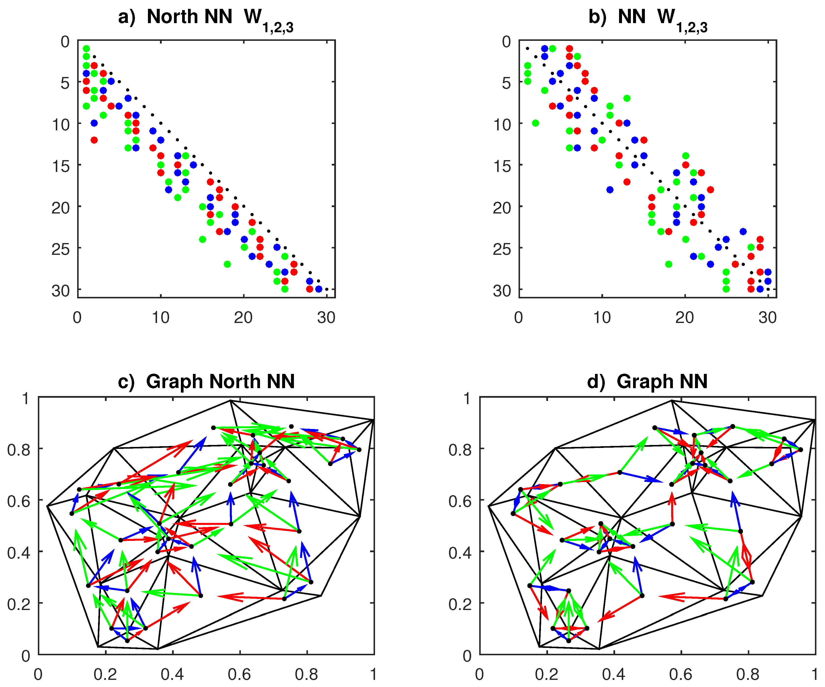
As an illustration of NN matrices, we simulate N=30 random points with and consider q=3 contiguous terms, see Figure f6. Under the north ordering of data, the entries of matrices are concentrated around the null main diagonal diag()=, and with the unilateral constraint the array is lower triangular. In order to obtain non-sparse matrices, LeSage and Pace (2004) ordered data according to the sum , but just used the simple NN rule. The matrices in Figure f6 yield SAR(3) models, but if they are combined as they provide constrained SAR(3,1). The analogous of the lattice model (4a) then becomes
The econometric literature often discusses models with autocorrelated errors, such as , e.g. Kelejian and Prucha (2007). Apart from estimation difficulties, it should be noted that they are encompassed by unconstrained SAR(2); indeed, the combined system involves just 2 spatial lags. In place of , it is better to insert into the model (13b) a lagged term on the exogenous part , that corresponds to in the model with errors. This is the Durbin model (LeSage and Pace, 2009), which is useful when are autocorrelated, i.e. have a non-random pattern.
When the matrix is lower triangular, the transfer function is always nonsingular and its inverse admits a convergent power expansion
This expression shows that the process , in the location s-th, depends on the values of the inputs and shocks in the north locations (), and with weights which decline with the distance. To appreciate this diffusion effect, note that when is strictly lower triangular, then also is lower triangular but with nonzero entries shifted away from the main diagonal. Hence, reflects the second-order contiguity (the neighbors of the neighbors), and so forth for the null matrix. The same feature, however, does not hold in non-triangular matrices, such as those based on the simple NN.
Figure 6.
Contiguity matrices and planar graphs of N=30 random centroids on the unit square [0,1]. Panels: (a,c) North nearest neighbors (NN); (b,d) Multidirection NN. Matrices: first NN (blue); second NN (red); third NN (green).
Figure 6.
Contiguity matrices and planar graphs of N=30 random centroids on the unit square [0,1]. Panels: (a,c) North nearest neighbors (NN); (b,d) Multidirection NN. Matrices: first NN (blue); second NN (red); third NN (green).
The unilateral model (14) corresponds to a time-series AR with unequally spaced observations. This feature is more clear in the presence of multiple lagged terms ; the suitable treatment is to weight the observations by the inverse Euclidean distance . The analog of the constrained model (15), with north NN linkage and with row normalization, is then given by
this also admits a vector representation as (13b) with triangular matrix , having q decreasing coefficients per row.
Alternatively, since the inverse distances decay too fast, one can use the exponential weights , with 01. In vector form, one has to define the diagonal matrices where contain the k-th north NN distances of the centroids. These arrays must be multiplied by the k-lag contiguity matrices , then summed as and finally normalized by rows. The resulting model is nonlinear in the parameters and requires iterative algorithms; however, the value of may be selected a-priori in the range [.9, 1), then the estimators compute the suitable value of .
3.1. Estimation Methods
Writing the models (14)-(16) in vector form, as , with and , where is the average of q-north NN terms, then the LS estimator of the parameters is given by
its unbiasedness follows from E by the sequential structure of the models, in particular E in the unilateral model.
To see what happens in detail, consider the LS estimator in matrix form
with regressors , the crucial term is . From Eq. (13c)
this term vanishes only if the trace (tr) of is 0, because
Now, in general holds if is strictly lower triangular, because is itself triangular with null diagonal.
As regards the convergence of LS estimator, multiplying Eq. (17) by , under regularity conditions (stability and existence of second-order moments) one has that , the covariance matrix of . Whereas
which is 0 if is triangular. Finally, under regularity conditions ( positive definite, and stationary) one has
where the convergence is in distribution (D), see Yao and Brockwell (2006).
For multilateral SAR models ( non-triangular), the LS is generally biased and inconsistent, and alternative estimators must be sought. The ML method may be suitable if the sample size N is moderate and the observations have Gaussian distribution. This estimator maximizes the log-likelihood function
which requires , i.e. the stability condition (LeSage and Pace, 2009, p.63). This requirement is not necessary in the LS method; moreover, numerical issues may arise in the optimization of Eq. (19), when computing , with the eigenvalues of . This techniques cannot be applied to triangular matrices, because =0 for all i.
Another method which is suitable for parameter estimates in multilateral is that of generalized moments (GM, Kelejian and Prucha, 1999); it arises by applying the instrumental variables (IV) method to the LS estimator (17). The first step is the definition of valid IVs: on the basis of the predictor decomposition , they may be given by . This provides the projection matrix and the regressors , which lead to the IV estimator . This solution is also of GM-type, as minimizes the functional , with the empirical moments and . In the following, we check the effectiveness of ML and GM estimators with simulation experiments.
3.2. Forecasting Functions
In forecasting, we have L out-of-sample units with value , whose coordinates and regressors are known for all . Their locations may be inside or outside the observed region; in both cases they are placed at the end of the data matrix . If the data are ordered in a certain direction (e.g. north-south with ), and all L units are outside the observed region, and in the same direction, then the weight matrix is nearly block-diagonal: , where is overlapped to for the contiguity of L units with the in-sample ones. In the other cases, it has a more complex structure, with triangular sub-matrices under the unilateral constraint
In any case, the estimation of parameters is performed with in-sample data and the matrix ; the other blocks will be used in forecasting.
The forecasting function of depends on the SAR representation used for ; Kelejian and Prucha (2007) also considered models with autocorrelated errors . In the reduced (MA) form (13c), the in-sample (fitted values) and out-of-sample forecasts are jointly computed as
where the contiguity matrix may have q-entries per row (the spatial lags) and may use non-uniform (IDW) weights. The matrix solution (20) is nearly automatic, but in absence of exogenous variables it provides constant forecasts.
The second predictor comes from the structural (AR) representation (13b); it is not automatic and must be managed sequentially by rows as Eq. (13a)
where are the l-th rows of the matrices . Note that for non-triangular , Eq. (21) involves missing values in the running vector . If these values are provided by Eq. (20), then the vector of observations and forecasts at l-th step becomes and, at the end , it will only contain the improved forecasts (21).
LeSage and Pace (2004) and Goulard et al. (2017) also discussed solutions based on the best linear unbiased predictor (BLUP) of Goldberger. This approach arises from the conditional mean and variance of Gaussian random vectors:
where is a subvector the predictor in Eq. (20) and come from the partition of the joint covariance matrix of , given by
The solution (22)-(23) requires a double matrix inversion: first and next ; in the presence of large N, this may introduce approximation errors. To reduce numerical instability, one may partition the simpler array and exploit the algebric relationship (see LeSage and Pace, 2008). The latter involves a single matrix inversion , of a submatrix of lower size . Finally, the conditional variance of the BLUP estimator may provide the dispersion of the forecasts (22)
this matrix requires the estimation of the variance , which can be carried out with the in-sample residuals of Eqs. (20).
As a final remark, notice that all formulae displayed until now can be extended to unconstrained SAR(q) models, by replacing the IR matrix with one of order q-th. For the predictors (20),(21) this yields the following dispersion
where the k-th lag contiguity matrices have size .
3.3. Simulations and Applications
To compare the various estimators, we perform simulation experiments of SAR models (13)-(16) on a random grid of N=150 points, unformly distributed in the unit square: , as in Figure f6c. We generate realizations of the process with independent inputs Uniform and Normal; parameters ; contiguity matrices with q=1,3 lags, with north NN and simple NN links. Subsequently, M=500 replications are fitted with LS, ML, GM estimators and relative biases, relative RMSE and p-values of Normality test were computed for the coefficents and then averaged. Note that relativization (e.g. bias) allows to sum the individual statistics so as to directly compare the various methods.
The results are reported in Table Section 2.2, where "variable grid" means that at each replication the centroids change and "variable weights" indicates that IDW are used in the matrices . The Durbin model includes a lagged term on the exogenous part, as , with coefficients . The software used for ML and GM estimatess is the Matlab package of LeSage and Pace (2009); it fits the Durbin model only with the ML method. Main conclusions from Table Section 2.2 are that ML and GM methods do not improve the LS estimates in the case of unidirectional (triangular) matrices. However, they significantly outperform LS in the multidirectional (e.g. simple NN) case; in particular, the ML method is the best. However, these results are not homogeneous as regards unbiasedness and efficiency of estimates, where the GM estimator may locally have smaller bias.
Forecasting. Unlike estimation, prediction evaluation of SAR methods cannot be based on pre-specified models and contiguity matrices, but it must refer to data generated from autonomous sources. As in the lattice case, we considered the random surfaces (11), sampled at random points , with ; however, the results are too favourable to unilateral SAR models. We then turn to the real USGS (2007) data in Figure 4, with n=340, m=455; we sample N=150 cells and withhold for forecasting L=30 outside, see Figure 7a. The fitted model is SAR (15) with q=3 and , and forecast functions (20)-(22); the unilateral model is estimated with LS and the multilateral one with ML.
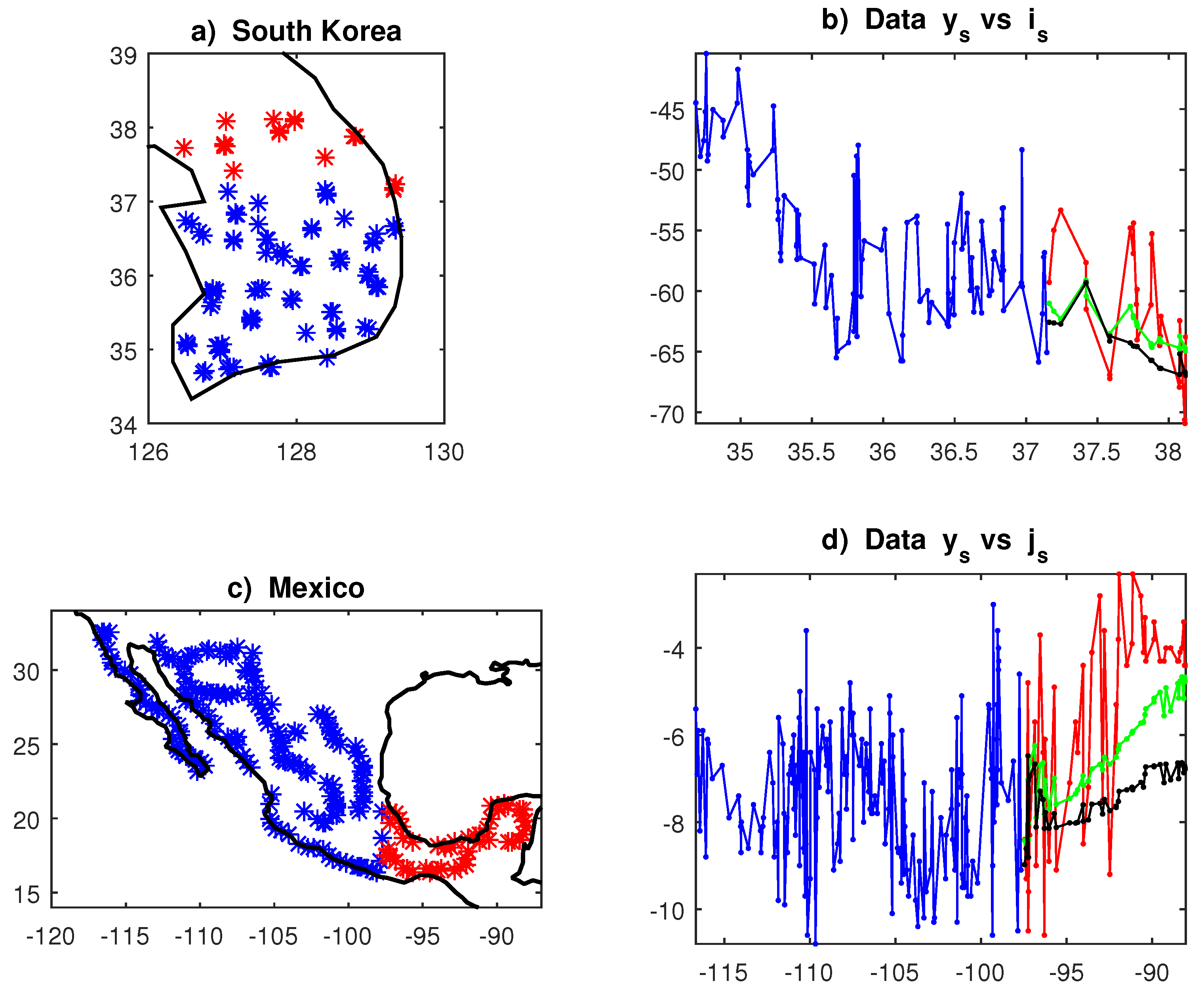
As a final application, we consider original point data concerning the measurement of stable isotopes of oxygen (O) and hydrogen (H) in the ground water. Mapping isoscapes is useful for physical monitoring of the hydrological cycle and for archeological and forensic investigations, regarding the path of people movement. We consider the datasets of Gautam et al. (2020), recorded in South-Korea in 2010, with N=130; and Moreiras Reynaga et al. (2021), recorded in Mexico in 2007, with N=234. We estimate SAR model (15) with q=3 for and = latitude, longitude, to forecast about 20% of observations; the results are in Tab. 6 and Fig. 8. They confirm the better performance of unilateral SAR models with the AR algorithm (21), especially when the data have significant autocorrelation (i.e. large ) and marked spatial trends (significant ). The reduction of MAPE staristics in Tab. 6 ranges from -18% in Korea to -38% in Mexico.

Table 6.
Parameter estimates (and T-statistics) and MAPE forecast statistics of the SAR model (15) with q=3 applied to the water isotope data of South Korea H (first block) and Mexico O (second block).
Table 6.
Parameter estimates (and T-statistics) and MAPE forecast statistics of the SAR model (15) with q=3 applied to the water isotope data of South Korea H (first block) and Mexico O (second block).
| Model | Method | ||||||||
|---|---|---|---|---|---|---|---|---|---|
| Unilateral | LS (17) | 123.7 | 0.337 | -0.557 | -2.51 | 4.28 | 0.069 | 0.065 | 0.065 |
| T-stat., | " | (1.70) | (4.72) | (-1.04) | (-3.37) | 0.478 | . | . | . |
| Multilat. | ML (19) | 97.9 | 0.622 | -0.376 | -1.98 | 3.53 | 0.080 | 0.079 | 0.079 |
| T-stat., | " | (1.69) | (9.46) | (-0.86) | (-3.41) | 0.645 | . | . | . |
| Unilateral | LS (17) | 4.30 | 0.636 | 0.089 | 0.093 | 1.28 | 0.377 | 0.369 | 0.370 |
| T-stat., | " | (1.69) | (8.17) | (3.19) | (2.72) | 0.336 | . | . | . |
| Multilat. | ML (19) | -0.85 | 0.479 | 0.053 | 0.101 | 1.26 | 0.600 | 0.597 | 0.588 |
| T-stat., | " | (-0.36) | (7.41) | (1.88) | (2.89) | 0.351 | . | . | . |
Figure 8.
Water isotopes data and SAR forecasts (22): Red=out-of-sample data, Green= forecasts with triangular; Black=forecasts with multilateral. Panels: a) South-Korea sample locations; b) Latitudinal view of Hydrogen isotope; c) Mexico sample locations; d) Longitudinal view of Oxigen isotope.
Figure 8.
Water isotopes data and SAR forecasts (22): Red=out-of-sample data, Green= forecasts with triangular; Black=forecasts with multilateral. Panels: a) South-Korea sample locations; b) Latitudinal view of Hydrogen isotope; c) Mexico sample locations; d) Longitudinal view of Oxigen isotope.
4. Conclusions
In this paper we have compared unilateral and multilateral SAR models in forecasting spatial data of both lattice and polygonal type. SAR systems are natural extensions of classical autoregressions, their difference is in the treatment of the spatial dependence: while unilateral models choose a single direction in space, as in time series, multilateral models consider multiple directions. These approaches lead to different contiguity matrices: triangular and sparse, usually computed with the nearest-neighbor approach. While triangular SAR models can be consistently estimated with least squares, multilateral SAR require maximum likelihood or method of moments; in the latter cases, numerical complexity increase with the dimension of the contiguity matrices. Instead, LS is not sensitive to the size of the lattice or the number of spatial units involved and can manage even large scale systems, see Eqs. (9) and (17). Simulation experiments on small-medium scale systems have shown that ML and GM are suitable for multilateral models, but LS is preferable for the unilateral ones, especially in presence of unstable systems ().
As in time series, unilateral models with data ordered in a certain direction, yield recursive (sequential) calculations, which allow simple and unconditional forecasting functions. Instead, multilateral models involve forward values which may be pre-estimated only with the reduced form (20). In the applications we have seen that out-of-sample forecasting of multilateral models benefits from the BLUP improvement (22), but the performance of the unilateral models with (21) remains better, see Tabs. 5 and 6. As regards the practical usage of SAR point forecasts, we mention the possibility to use them as alternatives to non-parametric smoothers, such as Kriging and Kernels, which are particularly sensitive to the border effects. Further, in order to overcome the limits of unidirectionality, one can estimate unilateral models in various directions (e.g. NS, SN, WE, EW), and then combine their forecasts. This solution is suitable for points inside the perimeter of the investigated area, but it can also be applied to external points by using diagonal paths (e.g. NE).
These are open topics for further research; other important areas of application of triangular contiguity matrices are to space-time (ST) data; in particular, to STAR and dynamic panel-data models (see Grillenzoni, 2004 and Copiello and Grillenzoni, 2021). In the latter reference it is shown how the unidirectional specification improves the performance even of robust (M-type) estimators, designed for data with outliers. Finally, the unilateral specification is also suitable for testing the Granger causality between spatial processes (e.g. Herrera et al., 2012) because it is related to diffusion effects which follow specific directions in the space.
Appendix A. Contiguity Matrices of SAR Lattice Models
We shows the derivation of the vector representation of a SAR model for lattice data, where p=spatial lag, q=number of units and r=number of parameters. Consider the array in Fig. A1 of size n=4, m=5, and a deterministic triangular scheme SAR(1,3,1): . Let be the column vectorization of length N=20; then, subject to fixed border conditions (first row and column), the vector representation becomes , where is the contiguity matrix in Fig. A1. In general, has m square blocks of size n on the main diagonal and blocks on the lower sub-diagonal, with central rows with q non-zero elements.
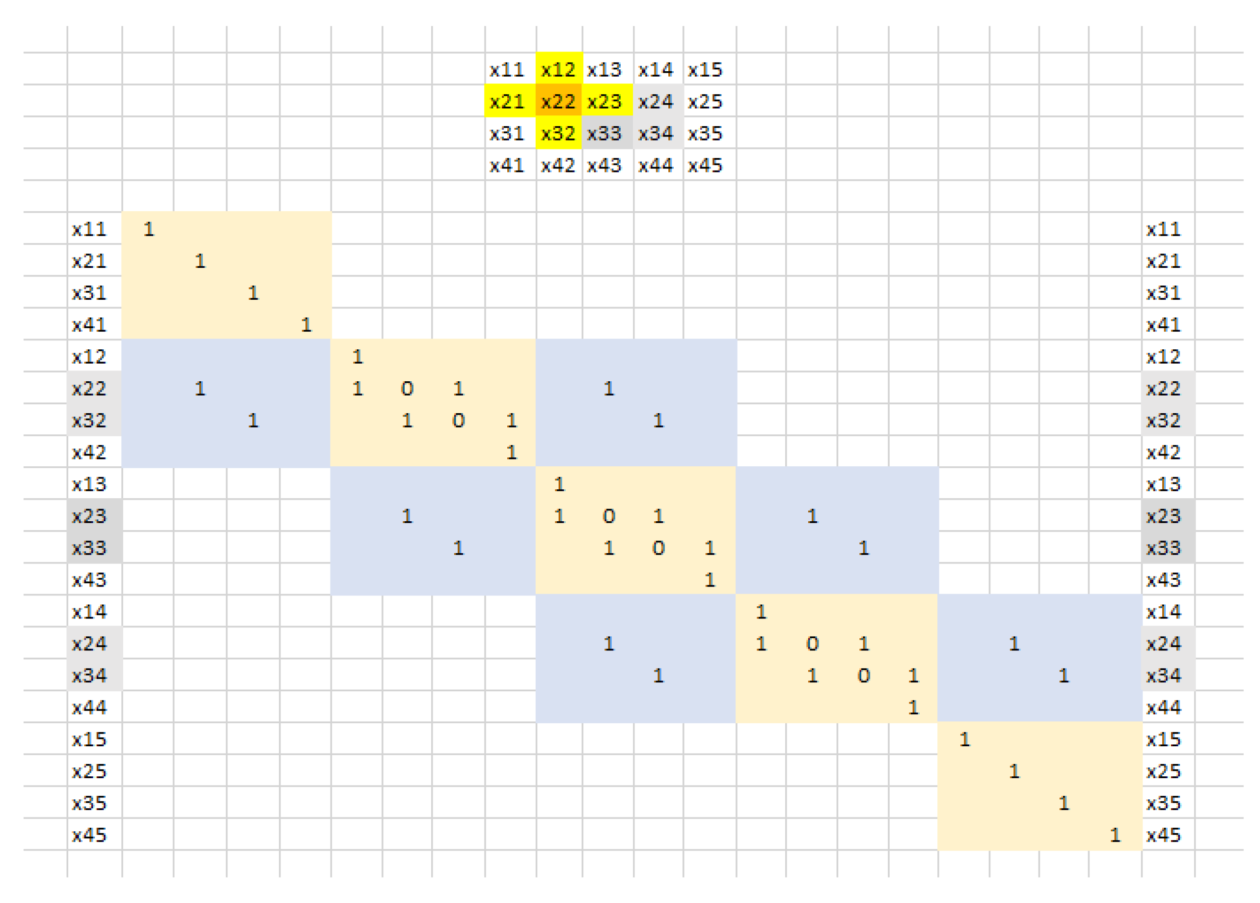
As regards the corresponding SAR(1,3,1) process , with border conditions =0, i.e. , its vector representation becomes , where the matrix is obtained by equating to zero all diagonal entries of in Figure A1. If r=q, the matrix is decomposed into r triangular matrices which provide . Analogously, Figure A2 shows the contiguity matrix for a rook model SAR(1,4,1); the corresponding is obtained by equating to zero all the diagonal entries.
Figure A1.
Vector representation of a triangular scheme on a lattice of size 4×5, with fixed border conditions.
Figure A1.
Vector representation of a triangular scheme on a lattice of size 4×5, with fixed border conditions.
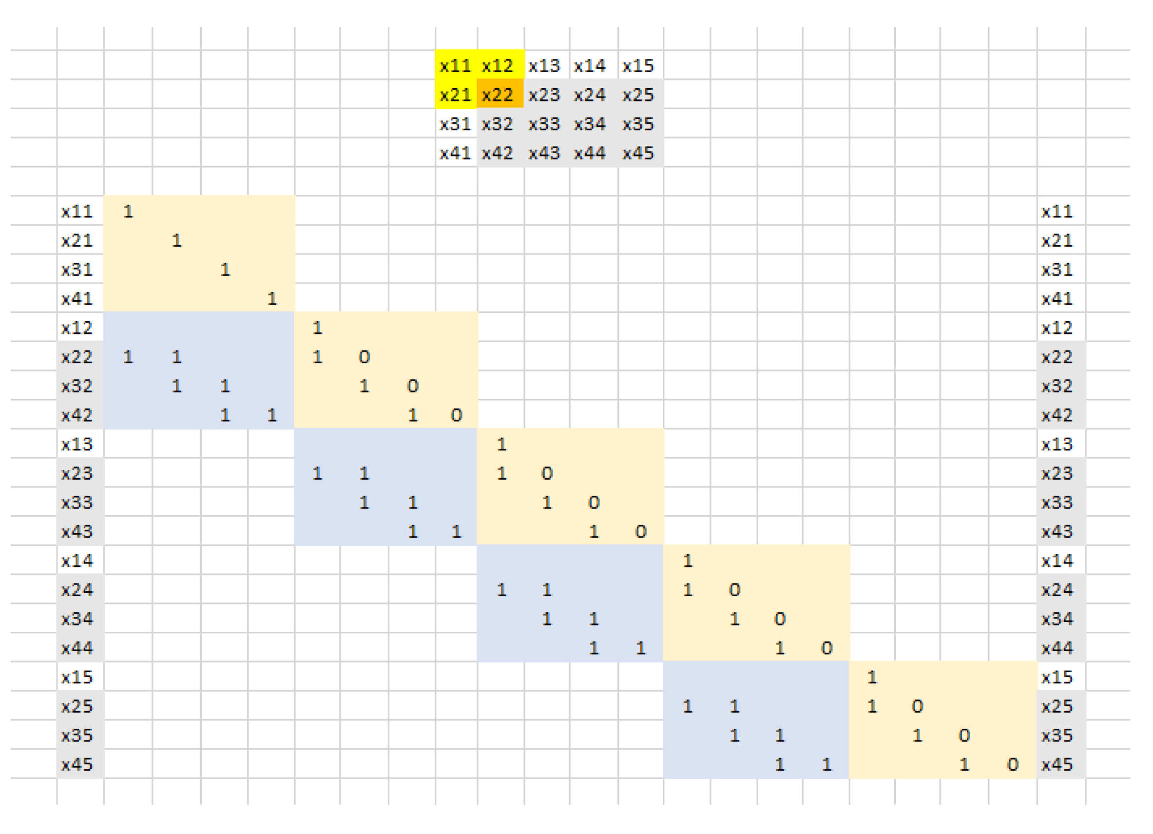
Figure A2.
Vector representation of a rook model on a lattice of size 4×5, with fixed border conditions.
Figure A2.
Vector representation of a rook model on a lattice of size 4×5, with fixed border conditions.
Appendix B. More Results on Surface Forecasting
We provide additional results of the experiment of Figure 4 and Table 2, which deals with forecasting a rough random surface (11) with models (4a,b). Figure A3 shows the forecasts of the vector algorithms (10b,c); as one can see, the results of the AR method (10b) are similar to those of the lattice function (10a), in Figure 4c,d. Instead, the forecasts of the reduced (MA) form (10c) are nearly constants in both models, due to the absence of exogenous variables, see Figure A3c,d.
Figure A3.
Forecasts of the surface in Figure 4b provided by the models (4a,b) and the predictors (10b,c).
Figure A3.
Forecasts of the surface in Figure 4b provided by the models (4a,b) and the predictors (10b,c).
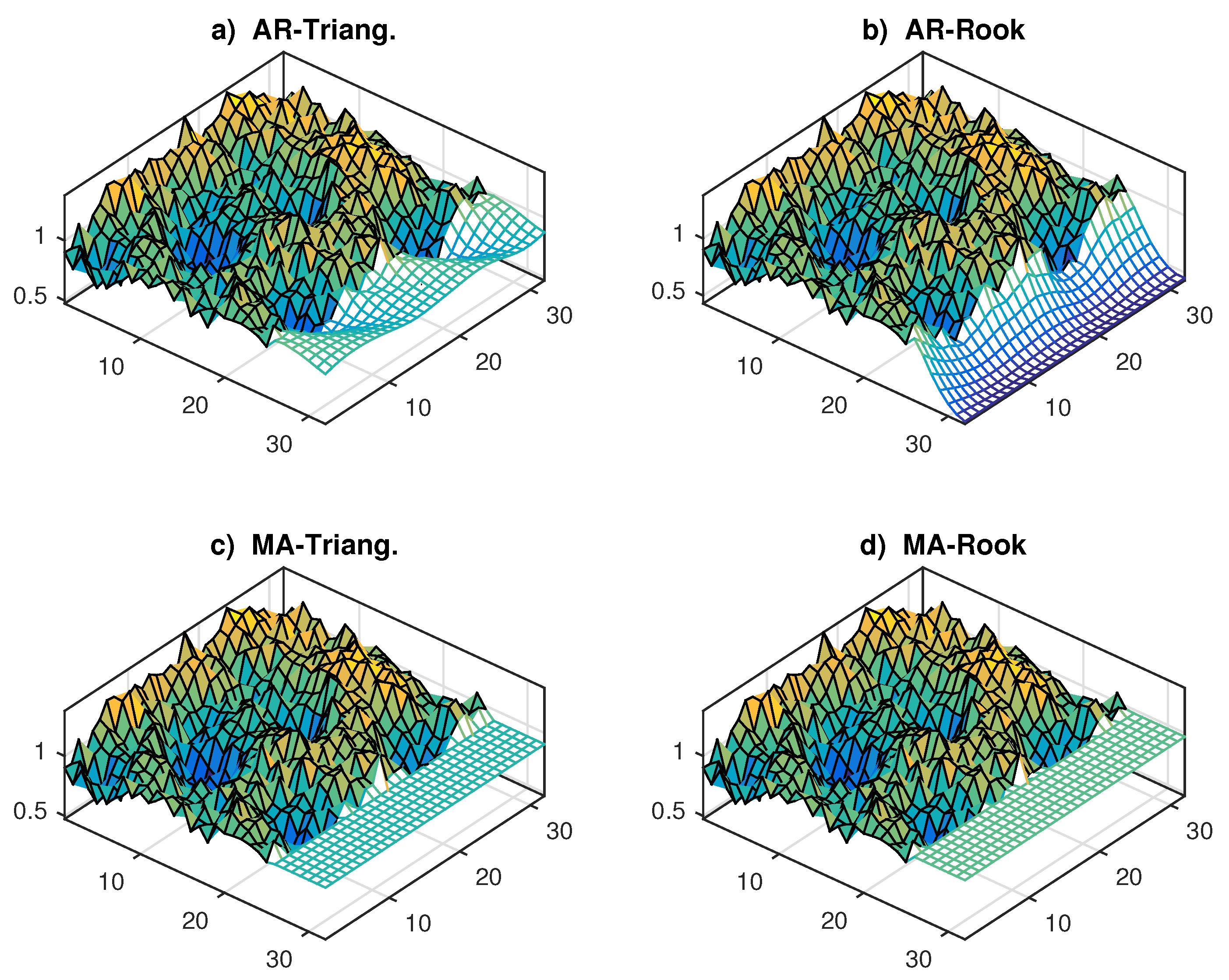
Table A1 provides the average values, over 10 replications of the surface (11), of the parameter estimates of the models (4a,b) and of their MAPE statistics. The results agree with those of Table 2, which regard a single replication; in particular, the forecasts of the triangular model (in lattice and vector form) are better than those of the rook scheme. The ML estimates are necessary for the multilateral model, but the unilateral one may also rely on the fast LS. In summary, the best methods, also from the graphical viewpoint, are unilateral models with the AR predictors.
Table A1.
Average values, over 10 replications of the surface (11), of parameter estimates (and T-statistics) and forecast statistics of the models (4a,b) with predictors (10a-c).
Table A1.
Average values, over 10 replications of the surface (11), of parameter estimates (and T-statistics) and forecast statistics of the models (4a,b) with predictors (10a-c).
| Model | Method | MAPE | |||
|---|---|---|---|---|---|
| Triang. (10a) | LS (2) | 0.118 (4.87) | 0.879 (37.0) | 0.641 | 0.116 |
| Rook (10a) | ML (19) | 0.231 (17.3) | 0.766 (58.2) | 0.738 | 0.183 |
| AR-Triang. (10b) | LS (9) | 0.107 (4.78) | 0.891 (40.6) | 0.668 | 0.117 |
| AR-Rook (10b) | ML (19) | " | " | " | 0.217 |
| MA-Triang. (10c) | LS (9) | " | " | " | 0.231 |
| MA-Rook (10c) | ML (19) | " | " | " | 0.584 |
References
- Anselin, L. Spatial Econometrics. In A Companionto Theoretical Econometrics; Baltagi, B.H.; Ed.; Blackwell Publishing, Oxford, 2003; pp. 310-330.
- Awang, N.; Shitan, M. Estimatingtheparametersofthesecondorderspatialunilateral autoregressivemodel. International Journal of Statistical Sciences 2006, 5, 37–58. [Google Scholar]
- Bao, Y.; Liu, X.; Yang, L. Indirectinferenceestimationforspatialautoregressions. Econometrics 2020, 8, 34. [Google Scholar] [CrossRef]
- Barbiero, T.; Grillenzoni, C. Planninganovelregionalmethanenetwork: Demandforecasting and economicevaluation. Energy Conversion and Management: X 2022, 16, 100294. [Google Scholar] [CrossRef]
- Basu, S.; Reinsel, G.C. Propertiesofthespatialnilateralfirst-orderARMAmodel. Advances in Applied Probability 1993, 25, 631–648. [Google Scholar] [CrossRef]
- Bhattacharyya, B.B.; Richardson, G.D.; Franklin, L.A. Asymptoticinferencefornearunitroots in spatialautoregression. Annals of Statistics 1997, 28, 173–179. [Google Scholar]
- Bustos, O.; Ojeda, S.; Vallejos, R. SpatialARMAmodelsanditsapplicationstoimagefiltering. Brazilian Jour.of Probab. Stat. 2009, 23, 141–165. [Google Scholar]
- Copiello, S.; Grillenzoni, C. Robustspacetimemodelingofsolarphotovoltaicdeployment. Energy Reports 2021, 7, 657–676. [Google Scholar] [CrossRef]
- Fingleton, B. Spatial Autoregression. Geograph. Anal. 2009, 41, 385–391. [Google Scholar] [CrossRef]
- Gautam, M.K.; Song, B.-Y.; Shin, W.-J.; Bong, Y.-S.; Lee, K.-S. DatasetsforspatialvariationofO and HisotopesinwatersandhairacrossSouthKorea. Data inBrief 2020, 30, 105666. [Google Scholar]
- Goulard, M.; Laurent, T.; Thomas-Agnan, C. Aboutpredictionsinspatialautoregressivemodels: optimal and almostoptimalstrategies. Spatial Economic Analysis 2017, 12, 304–325. [Google Scholar] [CrossRef]
- Granger, C.W.J. Usefulconclusionsfromsurprisingresults. J. Econom. 2012, 169, 142–146. [Google Scholar] [CrossRef]
- Grillenzoni, C. Adaptivespatio-temporalmodelsforsatelliteecologicaldata. Jour. of Agric. Biol. &Environ.Statistics 2004, 9, 158–180. [Google Scholar]
- Grillenzoni, C. Statisticsforimagesharpening. Statistica Neerlandica 2008, 62, 173–192. [Google Scholar] [CrossRef]
- Herrera, M.; Ruiz, M.; Mur, J. Someexamplesoftheuseofanewtestforspatialcausality. Estadística Espa ˜nola 2012, 54, 53–70. [Google Scholar]
- Jarque, C.M.; Bera, A.K. Atestfornormalityofobservationsandregressionresiduals. International Statistical Review 1987, 55, 163–172. [Google Scholar] [CrossRef]
- Kelejian, H.H.; Prucha, I.R. Ageneralizedmomentsestimatorfortheautoregressiveparameter in aspatialmodel. Internat. Econom.Rev. 1999, 40, 509–533. [Google Scholar] [CrossRef]
- Kelejian, H.H.; PruchaI, R. Therelativeefficienciesofvariouspredictorsinspatialeconometric models containingspatiallags Regional ScienceandUrbanEconomics 2007, 37, 363-374.
- Lee, L.F. Consistencyandefficiencyofleastsquaresestimationformixedregressive,spatial autoregressivemodels. Econometric Theory 2002, 18, 252–277. [Google Scholar] [CrossRef]
- Lee, L.F. Bestspatialtwo-stageleastsquaresestimatorsforaspatialautoregressivemodel with autoregressivedisturbances. Econometric Reviews 2003, 22, 307–335. [Google Scholar] [CrossRef]
- LeSage, J.P.; Pace, R.K. Modelsforspatiallydependentmissingdata. Journal of Real Estate Finance and Economics 2004, 29, 233–254. [Google Scholar] [CrossRef]
- LeSage, J.P.; Pace, R.K. (2008). Spatialeconometricmodels,prediction.In Shekhar, S.; Xiong, H.(eds), Encyclopedia of Geographical Information Science, 1095-1100. Springer:NewYork.
- LeSage, J.P.; Pace, R.K. IntroductiontoSpatialEconometrics. CRCPress,Taylor&Francis Group. 2009.
- Mojiri, A.; Waghei, Y.; Nili-Sani, H.R.; MohtashamiBorzadaran, H.R. Thestationaryregions for theparameterspaceofunilateralsecond-orderspatialARmodel. Random Operatorsand Stochastic Equations 2018, 26, 185–191. [Google Scholar] [CrossRef]
- Mojiri, A.; Waghei, Y.; Nili-Sani, H.R.; Mohtashami Borzadaran, H.R. Non-stationaryspatial autoregressivemodelingforthepredictionoflatticedata. Communications inStatistics-Simulation and Computation 2021, 100, 1–13. [Google Scholar]
- MoreirasReynaga, D.K.; Millaire, J.-F.; ChávezBalderas, X.; RománBerrelleza, J.A.; LópezLuján, L.; Longstaffe, F.J. BuildingMexicanisoscapes:Oxygenandhydrogenisotopedataof meteoric watersampledacrossMexico. Data inBrief 2021, 36, 107084. [Google Scholar]
- Sheffield, S. Whatisarandomsurface?Proc.Int.Cong.Math.2022,InternationalMathemati-cal Union, EMSPress. 2022.
- Sjodin, B. (2017), GenerateRandomSurfacesinCOMSOLMultiphysics(R). Avalibaleat:https://www.comsol.
- Tjøstheim, D. StatisticalSpatialSeriesModellingII:SomefurtherResultsinUnilateral Processes. Advances in Applied Probability 1983, 15, 562–684. [Google Scholar] [CrossRef]
- USGS. U.S. Geological Survey, Digital Elevation Models (DEMs). 2017. Avalilableat: https://www.sciencebase.
- Yao, Q.; Brockwell, P.J. Gaussian Maximum Likelihood Estimation for ARMAModels II: Spatial Processes. Bernoulli 2006, 13, 403–429. [Google Scholar]
Figure 1.
Examples of lattice (a,b) and polygonal (c,d) data, with unilateral (a,c) and multilateral (b,d) spatial dependence schemes, with respect to their nearest neighbors.
Figure 1.
Examples of lattice (a,b) and polygonal (c,d) data, with unilateral (a,c) and multilateral (b,d) spatial dependence schemes, with respect to their nearest neighbors.
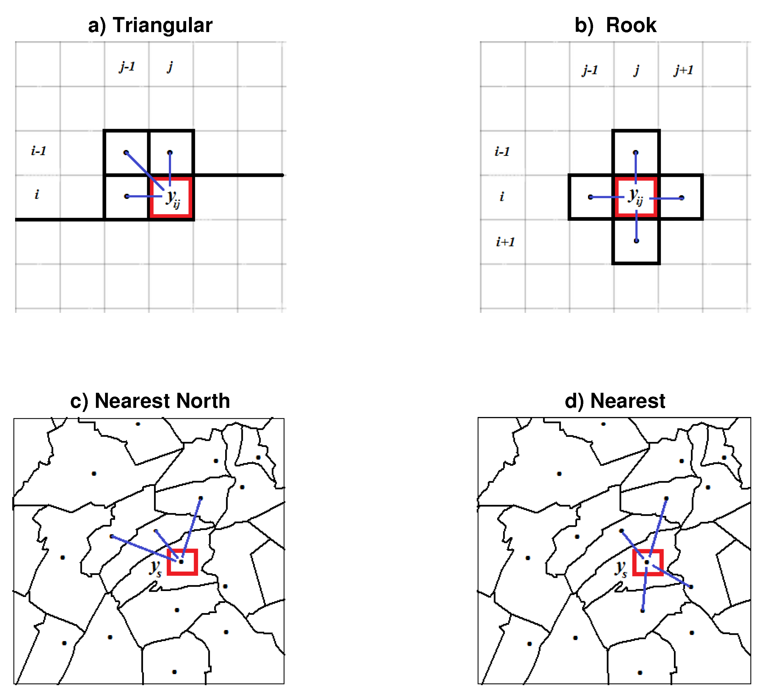
Figure 2.
Contiguity matrices of the models (4a,b) on a lattice of size n=4, m=7. Red dots have value 1 and correspond to border values; while the blue are 1/3 in Panel (a) and 1/4 in Panel (b); see Appendix A.
Figure 2.
Contiguity matrices of the models (4a,b) on a lattice of size n=4, m=7. Red dots have value 1 and correspond to border values; while the blue are 1/3 in Panel (a) and 1/4 in Panel (b); see Appendix A.
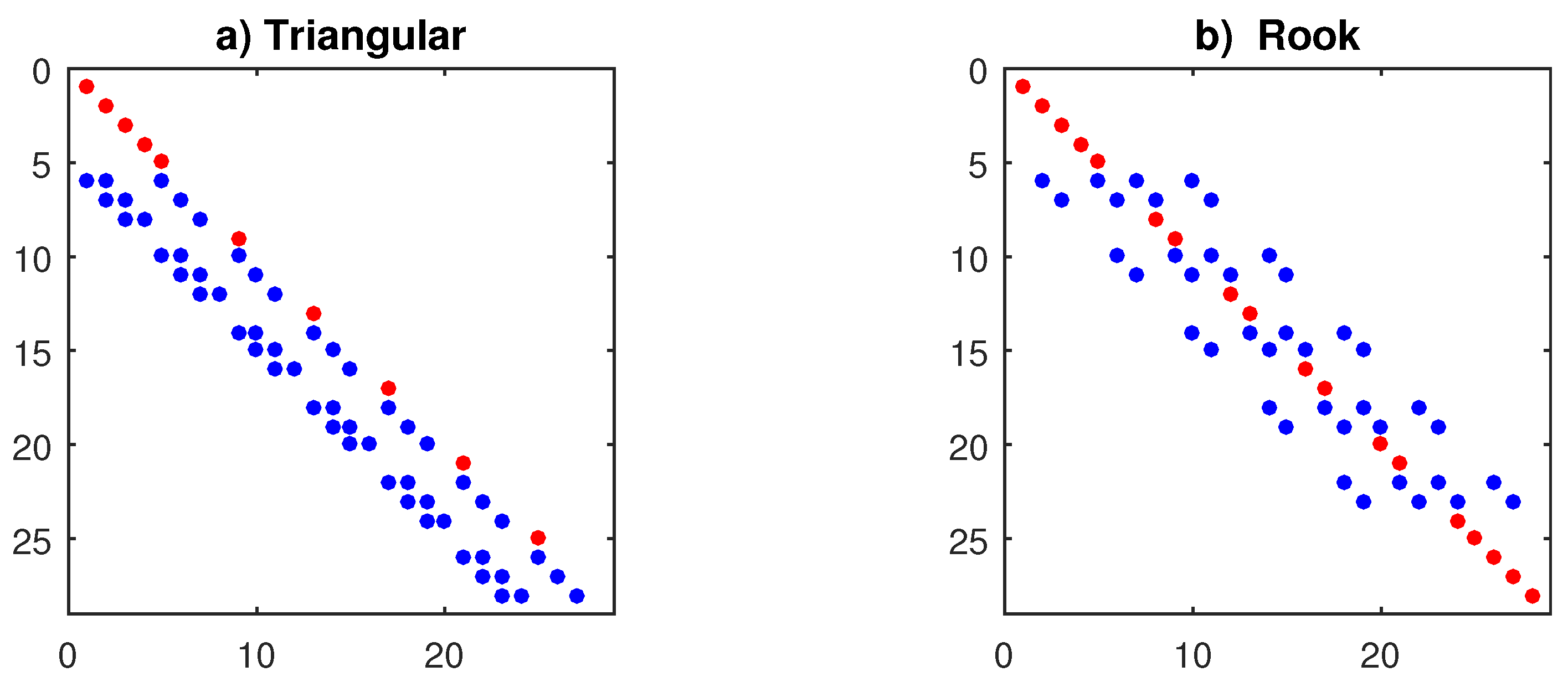
Figure 3.
Distribution of LS and ML estimates in 200 replications of the SAR models (4a,b) with =1, =1 (green), and mean values of (red): Panels (a,b) LS (9) of model (4a); Panels (c,d) ML (19) of model (4b).
Figure 3.
Distribution of LS and ML estimates in 200 replications of the SAR models (4a,b) with =1, =1 (green), and mean values of (red): Panels (a,b) LS (9) of model (4a); Panels (c,d) ML (19) of model (4b).
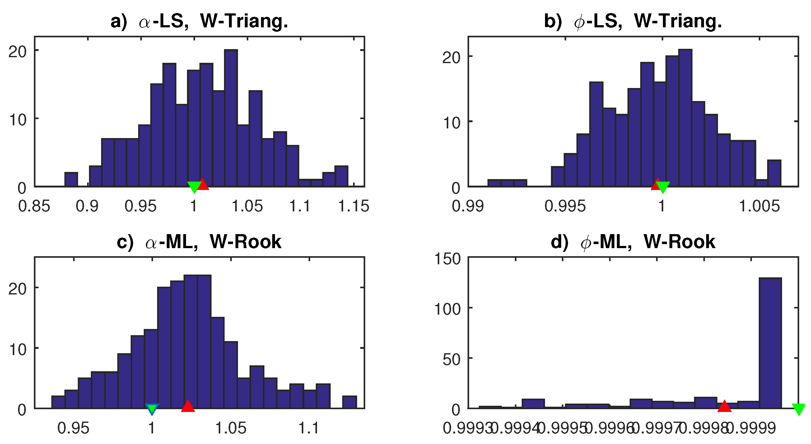
Figure 4.
Panels (a,b): Simulation of the random surface (11) of size n=m=32. Panels (c,d): Out-of-sample forecasts of (:,26:32) with models (4a,b) and predictor (10a).
Figure 4.
Panels (a,b): Simulation of the random surface (11) of size n=m=32. Panels (c,d): Out-of-sample forecasts of (:,26:32) with models (4a,b) and predictor (10a).
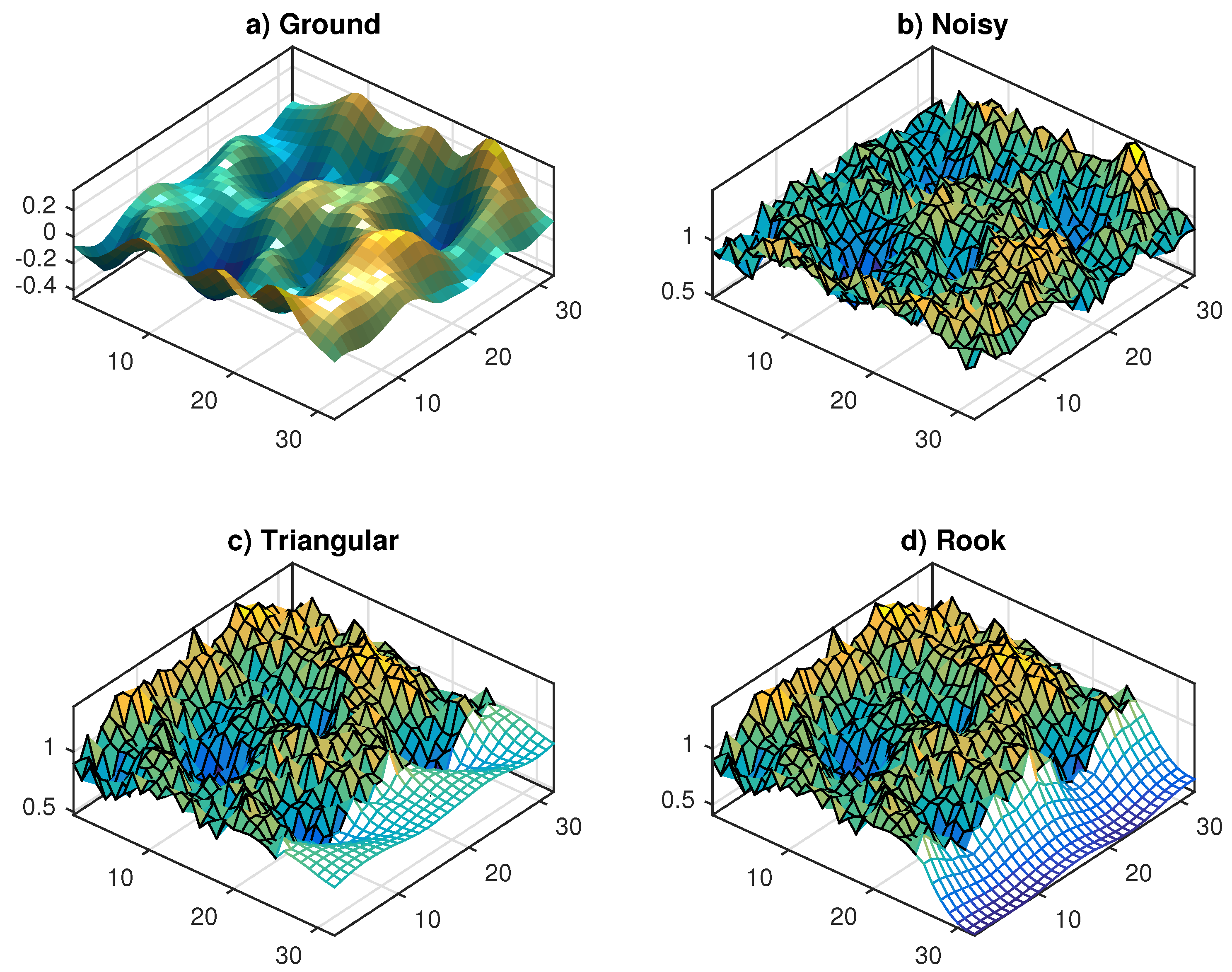
Figure 5.
Application of SAR models (4a,b) with quadratic trend to USGS (2027) data: out-of-sample forecasts of the image portion (:,401:455).
Figure 5.
Application of SAR models (4a,b) with quadratic trend to USGS (2027) data: out-of-sample forecasts of the image portion (:,401:455).
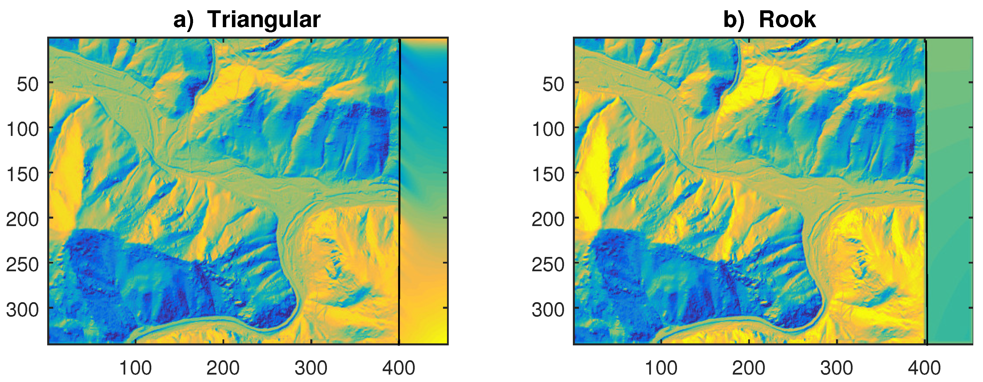
Figure 7.
Graphical results of a single replication of the estimates in Table 5: a) Random sampling of USGS surface (points to forecast are in red); b) Longitudinal display of data and forecasts (21) (unilateral=green, multilateral=black); c) Contiguity matrix of the unilateral model with q=3; d) Contiguity matrix of the multilateral model.
Figure 7.
Graphical results of a single replication of the estimates in Table 5: a) Random sampling of USGS surface (points to forecast are in red); b) Longitudinal display of data and forecasts (21) (unilateral=green, multilateral=black); c) Contiguity matrix of the unilateral model with q=3; d) Contiguity matrix of the multilateral model.
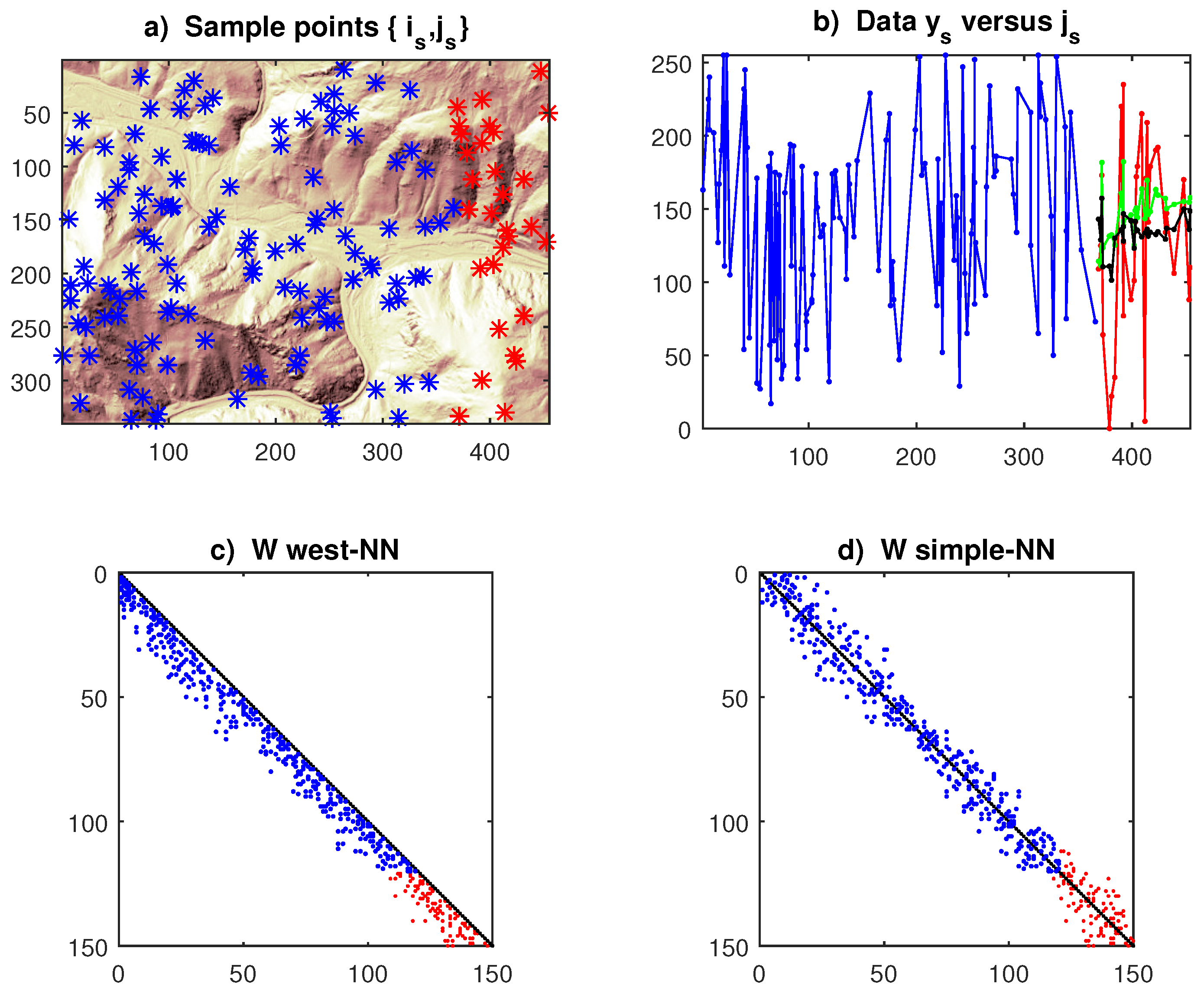
Table 1.
Performance of LS (9) and ML (19) estimators applied to triangular and rook SAR models (4a,b) with n=m=32: R-bias=relative bias, R-RMSE=relative root mean squared error, N-test=p-values of the normality test. The bold character enhances the best methods (LS or ML) over model classes (Triang. and Rook).
Table 1.
Performance of LS (9) and ML (19) estimators applied to triangular and rook SAR models (4a,b) with n=m=32: R-bias=relative bias, R-RMSE=relative root mean squared error, N-test=p-values of the normality test. The bold character enhances the best methods (LS or ML) over model classes (Triang. and Rook).
| Method | LS | Triang. | LS | Rook | ML | Triang. | ML | Rook | |
|---|---|---|---|---|---|---|---|---|---|
| Stat. | |||||||||
| R-bias | 0.015 | 0.013 | 0.279 | 0.325 | 0.295 | 0.324 | 0.014 | 0.014 | |
| R-RMSE | 0.078 | 0.078 | 0.289 | 0.334 | 0.302 | 0.329 | 0.062 | 0.066 | 0.5 |
| N-test | >0.5 | 0.415 | 0.456 | 0.267 | 0.319 | 0.065 | 0.221 | 0.138 | |
| R-bias | 0.021 | 0.007 | 0.330 | 0.134 | 0.372 | 0.148 | 0.023 | 0.008 | |
| R-RMSE | 0.088 | 0.032 | 0.339 | 0.136 | 0.384 | 0.153 | 0.074 | 0.028 | 0.75 |
| N-test | >0.5 | >0.5 | 0.413 | 0.135 | >0.5 | >0.5 | 0.192 | 0.052 | |
| R-bias | 0.007 | 0.0003 | 0.004 | 0.0001 | 0.049 | 0.003 | 0.023 | 0.0002 | |
| R-RMSE | 0.053 | 0.003 | 0.054 | 0.0004 | 0.067 | 0.004 | 0.043 | 0.0002 | 1 |
| N-test | >0.5 | >0.5 | 0.412 | 0.119 | 0.126 | 0.001 | 0.092 | 0.001 | |
| R-bias | 0.0057 | 0.0001 | 0.003 | 0.0000 | 0.510 | 0.024 | 2.270 | 0.023 | |
| R-RMSE | 0.047 | 0.002 | 0.035 | 0.0001 | 0.512 | 0.024 | 2.286 | 0.024 | 1.025 |
| N-test | >0.5 | >0.5 | >0.5 | 0.001 | >0.5 | 0.001 | 0.450 | 0.001 |
Table 2.
Parameter estimates (with T-statistics in parentheses) of SAR models (4a,b) on the surface (:,1:25) in Figure 4b, and forecast statistics on the data (:,26:32).
Table 2.
Parameter estimates (with T-statistics in parentheses) of SAR models (4a,b) on the surface (:,1:25) in Figure 4b, and forecast statistics on the data (:,26:32).
| Model | MAPE | ||||||
|---|---|---|---|---|---|---|---|
| Triang. (4a) | LS | 0.096 (4.45) | 0.893 (40.3) | . | . | 0.686 | 0.143 |
| Triang. (4a) | ML | 0.247 (15.2) | 0.739 (45.1) | . | . | 0.665 | 0.125 |
| SAR(1,3,3) | LS | 0.094 (4.42) | 0.448 (13.3) | 0.097 (2.69) | 0.352 (10.1) | 0.701 | 0.140 |
| Rook (4b) | LS | –0.008 (-0.39) | 1.008 (50.6) | . | . | 0.788 | 0.864 |
| Rook (4b) | ML | 0.198 (16.3) | 0.795 (64.9) | . | . | 0.753 | 0.224 |
Table 3.
Estimates of SAR models with bivariate polynomials applied to the USGS (2017) image: (:,1:400) in-sample data, (:,401:455) out-of-sample.
Table 3.
Estimates of SAR models with bivariate polynomials applied to the USGS (2017) image: (:,1:400) in-sample data, (:,401:455) out-of-sample.
| Model | MAPE | ||||||||
|---|---|---|---|---|---|---|---|---|---|
| Triang. (4a) | 8.50 | 0.961 | –0.024 | –0.011 | 11e-5 | 43e-7 | –88e-7 | 338.4 | 0.848 |
| T-stat., | 25.56 | 104.9 | –10.58 | –5.47 | 22.55 | 0.735 | –2.07 | 0.913 | . |
| Rook (4b) | –6.12 | 1.026 | 0.007 | 0.016 | –58e-6 | 17e-6 | –17e-6 | 88.15 | 1.362 |
| T-stat., | –35.82 | 214.0 | 6.29 | 15.87 | –22.80 | 5.50 | –7.82 | 0.977 | . |
Table 4.
Results of the simulation experiments on the SAR systems (13)-(15) with spatial lags q=1-3 and single . The statistics are average values (over ) of relative biases, relative RMSE and p-value of N-test. Bold characters indicate the best results.
Table 4.
Results of the simulation experiments on the SAR systems (13)-(15) with spatial lags q=1-3 and single . The statistics are average values (over ) of relative biases, relative RMSE and p-value of N-test. Bold characters indicate the best results.
| W | North NN | Simple NN | ||||||
|---|---|---|---|---|---|---|---|---|
| Estimator | LS | ML | GM | LS | ML | GM | lags | |
| Ave. Rbias | 0.0205 | 0.1338 | 0.0235 | 0.1363 | 0.0287 | 0.0216 | 0.65 | 1 |
| Ave. RRMSE | 0.1336 | 0.2402 | 0.1831 | 0.1887 | 0.1343 | 0.1581 | ||
| Ave. Ntest | 0.3218 | 0.2983 | 0.1675 | 0.1561 | 0.3401 | 0.3337 | ||
| Ave. Rbias | 0.0077 | 0.1208 | 0.0098 | 0.1232 | 0.0400 | 0.0075 | 0.65 | 1 |
| Ave. RRMSE | 0.1396 | 0.2445 | 0.1924 | 0.1873 | 0.1430 | 0.1609 | (Variable | |
| Ave. Ntest | 0.3274 | 0.3554 | 0.2291 | 0.1637 | 0.2499 | 0.1626 | grid) | |
| Ave. Rbias | 0.0340 | 0.1330 | 0.0217 | 0.1324 | 0.0259 | 0.0376 | 0.65 | 3 |
| Ave. RRMSE | 0.1586 | 0.2416 | 0.2365 | 0.1998 | 0.1390 | 0.2035 | ||
| Ave. Ntest | 0.2442 | 0.2612 | 0.0936 | 0.1811 | 0.2559 | 0.0960 | ||
| Ave. Rbias | 0.0298 | 0.1289 | 0.0228 | 0.1487 | 0.0208 | 0.0343 | 0.65 | 3 |
| Ave. RRMSE | 0.1518 | 0.2360 | 0.2228 | 0.2088 | 0.1326 | 0.1963 | (IDW | |
| Ave. Ntest | 0.2530 | 0.2561 | 0.1673 | 0.1805 | 0.2900 | 0.1736 | weights) | |
| Ave. Rbias | 0.0312 | 0.0980 | 0.0248 | 0.0581 | 0.0109 | 0.0164 | 0.95 | 3 |
| Ave. RRMSE | 0.1475 | 0.2514 | 0.3190 | 0.1208 | 0.1086 | 0.1648 | ||
| Ave. Ntest | 0.1516 | 0.1678 | 0.0010 | 0.2611 | 0.3033 | 0.1601 | ||
| Ave. Rbias | 0.0663 | 0.3405 | . | 0.3333 | 0.0704 | . | 0.65 | 3 |
| Ave. RRMSE | 0.2849 | 0.4659 | . | 0.4141 | 0.2764 | . | (Durbin | |
| Ave. Ntest | 0.2584 | 0.3891 | . | 0.1286 | 0.1313 | . | model) |
Table 5.
Average Values, over 100 Replications, of Parameter Estimates (and T-statistics) and MAPE Forecast Statistics of SAR Model (15) on Random Samples of USGS (2007) Data.
Table 5.
Average Values, over 100 Replications, of Parameter Estimates (and T-statistics) and MAPE Forecast Statistics of SAR Model (15) on Random Samples of USGS (2007) Data.
| Model | Method | ||||||||
|---|---|---|---|---|---|---|---|---|---|
| Unilateral | LS (17) | 68.4 | 0.543 | 0.012 | -0.018 | 54.3 | 0.948 | 0.815 | 0.830 |
| -stat., | " | (3.0) | (5.1) | (0.21) | (-0.31) | 0.213 | . | . | . |
| Multilat. | ML (19) | 76.5 | 0.492 | 0.005 | -0.009 | 50.2 | 0.996 | 0.951 | 0.899 |
| -stat., | " | (4.2) | (6.3) | (0.06) | (-0.19) | 0.328 | . | . | . |
Disclaimer/Publisher’s Note: The statements, opinions and data contained in all publications are solely those of the individual author(s) and contributor(s) and not of MDPI and/or the editor(s). MDPI and/or the editor(s) disclaim responsibility for any injury to people or property resulting from any ideas, methods, instructions or products referred to in the content. |
© 2024 by the authors. Licensee MDPI, Basel, Switzerland. This article is an open access article distributed under the terms and conditions of the Creative Commons Attribution (CC BY) license (http://creativecommons.org/licenses/by/4.0/).
Copyright: This open access article is published under a Creative Commons CC BY 4.0 license, which permit the free download, distribution, and reuse, provided that the author and preprint are cited in any reuse.


