Submitted:
11 August 2024
Posted:
13 August 2024
You are already at the latest version
Abstract
BACKGROUND: Scoliosis is a widespread musculoskeletal disorder of bending and twisting of spine. In this medical ailment, spine curves to the side and even in severe cases it can twist and can take several bends. For the diagnosis and treatment of scoliotic patients, the Cobb’s angle is a critical marker of the body’s curvature. OBJECTIVE: There are many researches that have been conducted to automate the manual measurement of the angle and every investigation has their own limita- tions. METHODS: This paper presents a method for precisely measuring the Cobb’s an- gle using deep learning based techniques. Mainly it comprises of feature enhance- ment of augmented dataset, a bespoke code for landmark estimation on the spine, segmentation model based on the U-Net architecture and a custom code for Cobb’s angle measurement. These measured angles are then compared to the given angles for the segmentation on biomedical (X-ray) images. RESULTS: The findings demonstrate that the proposed technique offers an auto- mated and impartial way for precisely measuring this angle with an overall accu- racy of 97% and Root Mean Square Error (RMSE) of 4.99, which can lower the variability, facilitate early detection, accurate diagnosis, and monitoring of scolio- sis progression. Additionally, it aids in the treatment planning and evaluating treat- ment outcomes. CONTRIBUTION: By leveraging the applications of Cobb’s angle measurement, healthcare professionals can enhance the quality of care and can improve long-term outcomes for individuals with scoliosis.
Keywords:
Scoliosis
; Cobb’s Angle
; Land-marking
; Segmentation
; X-rays
; Deep Learning
; Contrast Adaptive Histogram Equalization (CLAHE)
; Serialization
; Deserialization
Introduction
The spinal abnormality known as scoliosis, affects the spine’s curvature, causing improper rotation and lateral deformation [1]. Scoliosis can affect people of all ages, genders, and ethnicities. Its prevalence rates vary based on different factors, such as geographic location, race, and age [2,3]. There are different types of scoliosis, including idiopathic, congenital, neuromuscular, and degenerative scoliosis based on the the root cause and vertebrae involved [4]. The majority of the cases of scoliosis, or of occurrences, are idiopathic, and they often manifest during adolescence. The precise root cause of idiopathic scoliosis is unknown, although environmental and genetic variables such as hormone imbalances, neuromuscular abnormalities, and development disruptions are considered to play a vital role [1].
The frequency of scoliosis in the general population is between and while it can occur at any age, it is most frequently detected in adolescence [2,5,6,7,8,9]. It can cause various physical, functional, and psychological impairments, ranging from mild to severe, depending on the severity of the curvature and the affected regions of the spine. Common symptoms of scoliosis include back pain, spinal stiffness, muscle imbalances, respiratory and cardiovascular dysfunction, reduced mobility, and poor posture [10,11].
In severe cases of scoliosis, significant cosmetic deformity is observed by affecting the quality of life of patients. Moreover, the afterwards treatment of scoliosis is quite expensive including diagnostic tests, therapeutics, surgeries, and ongoing monitoring [12,13]. Figure 1 gives the scoliotic view of a normal spine.
Assessing the severity and progression of scoliosis is critical for guiding treatment decisions and predicting outcomes. Its early detection allows for treatment to begin before the curve in the spine becomes severe. Literature [2,14] has shown that early detection and treatment of scoliosis can lead to better outcomes and reduce the need for surgery. Another reason why scoliosis detection is crucial is that untreated scoliosis can lead to complications such as chronic pain, difficulty in breathing, and even heart problems. Studies have shown that scoliosis can negatively affect a person’s quality of life, if left untreated [4,15,16].
By detecting scoliosis early and treating it appropriately, individuals can maintain a better quality of life and continue to participate in their normal activities. Conservative treatment approaches such as bracing have been shown to be effective in preventing progression of scoliosis [1,17,18]. Finally, scoliosis detection can increase awareness about the condition and encourage more people to seek treatment, if necessary. Health organizations such as the National Institute of Arthritis and Musculoskeletal and Skin Diseases provide information and resources to help people understand scoliosis and its treatment [1,19].
The gold standard for scoliosis evaluation is the Cobb’s angle, which gauges the degree of spine curvature [20]. The angle between the upper end-plate of the most severely twisted vertebra above the curve’s apex and the lower end-plate of that vertebra below the apex is known as the Cobb’s angle [12,18]. Figure 2 shows the measurement of Cobb’s angle. However, accurate and reliable estimation of the Cobb’s angle can be challenging, as it requires the identification of specific vertebral landmarks by human experts [12,21], which can be subjected to inter-observer variability and measurement errors. Moreover, traditional methods of Cobb’s angle measurement may not be sensitive enough to detect subtle changes in spinal curvature, particularly in patients with early onset scoliosis [22].
Given the difficulties in measuring Cobb’s angles manually, interest in creating automated and objective evaluation techniques is rising. Recent advances in deep learning methods have shown significant results in automating the process of Cobb’s angle measurement, potentially improving its accuracy and efficiency [24]. By training deep learning algorithms on large datasets, researchers can develop automated methods that recognize and localize vertebral landmarks automatically, enabling rapid and accurate evaluation of the Cobb’s angle [25].
The potential of deep learning in improving the accuracy and efficiency of Cobb’s angle measurement has important implications for the diagnosis and management of scoliosis, as it can help identify patients who are at risk of curve progression and require close monitoring or intervention. Additionally, automated measurement methods can reduce measurement errors and inter-observer variability. However, the accuracy and reliability of automated methods pose challenges due to noisy dataset, computational complexity, and the need for enhanced algorithms. The major contributions of this research include:
- Accurate Cobb’s Angle Measurement: By leveraging advanced mathematical techniques and innovative algorithms, this proposed technique surpasses existing methods in terms of precision and reliability, offering clinicians a more robust and trustworthy measurement tool.
- Noise-Resistant Dataset Analysis: Dealing with noisy dataset is a ubiquitous challenge in scoliosis assessment. To overcome this hurdle, we have meticulously designed algorithm that is trained in the context to obtain generalization and perform on noisy dataset, leading to more accurate and consistent Cobb’s angle measurements on real world dataset.
- Reduced Computational Complexity:By employing streamlined and innovative computational techniques, we have significantly reduced the computational complexity associated with accurate angle determination, thereby enhancing efficiency and practicality in clinical practice.
- Enhanced Algorithm Design: Research contributions extend beyond accuracy and efficiency. We have also focused on improving the overall design of the algorithm to accommodate diverse scoliosis cases without compromising on performance.
Specifically, a deep learning algorithm is trained on a large dataset of X-ray images of scoliotic spines and evaluated its performance in measuring the Cobb’s angle, comparing it to measurements made by human experts. The results demonstrate the potential of deep learning in improving the accuracy and efficiency of this angle measurement, and the implications of the findings are also discussed for diagnosing and treating scoliosis.
The structure of this paper is as follows: First, the significant previous work is discussed in Section 1. Than proposed technique is explained in Section 2 with the implementation details in Section 3. While implementation and results are covered in Section 4 with a discussion on them. Section 5 concludes the work and possible future directions.
1. Literature Review
Spine provides structural support to body and safeguards the spinal cord. Its malformation such as curvature is scoliosis. Image analysis techniques [27] and mechanical approaches used for its detection and evaluation are time consuming and more prone to errors. Manual measurement of angle performed by experts face multiple challenges like patient posture during the process, tissue contrast in scans etc. Such challenges make it more difficult to correctly identify the extent of curvature. In this section, a general overview of prevalent researches in the area is covered. Specifically, we will discuss the significant work done using four categories of dataset i.e.,
- X-ray images
- CT-scans
- Ultrasonographs
- Radiographs
Experiments performed for manual measurements [27] shows an error rate of to degree variation. As far as supervised methods are concerned, these are also not very much effective in medical fields because they have poor accuracy due to information loss during process [28]. As a whole, studies show that these techniques still needs improvements to get better results and deep learning based methods perform much better.
In [29], Cobbâs angle was measured by using Convolutional Neural Networks (CNNs) based framework. Experimentation was performed on 210-grey scaled X-ray images having and 10 training, testing and validation sets, respectively. In the detailed structure of technique, Region of Interests (ROI) found for noise reduction using Aggregated Channel Feature (ACF), directly extracts the features from image pixels and their intensity values. From this intensity based ROI, spine area was identified as it has higher intensity and its edges were determined. After defining the spine edges, vertebral detection was most crucial stage which further lead to vertebral segmentation section. For segmentation, U-net based structure was modified. At the encoder side, convolution with filter of Rectified Linear Unit (ReLU) normalization and down-sampling was done for feature extraction to build feature map and then later on in the decoder section up-sampling and concatenation was performed. The measurement coefficients used were Dice Similarity Coefficient and Jaccard Similarity Index. To calculate the Cobbâs angle of the segmented vertebrae images, maximum bounding box method was used. This proposed framework was based on residual network and compared to Dense U-Net and Standard U-Net based architecture. From all of them, Residual based architecture surpasses others showing mean segmentation accuracy. A T-Test was also performed for framework and for the comparison of manually measured results. However, this research did not use any image reconstruction and enhancement technique to eliminate the noise which affected the accuracy.
CNNs was also used as to segment the center line of spinal column on MICCAI dataset [30]. Then to calculate the angle, derivatives were taken. Mean Absolute Error (MAE) of angle were observed to degree with a limitations of technique like cropping the image close to spine which lead to a major issue for automated assessment with a larger running time.
These time taking measurements urged to develop some automated techniques, which is done with the help of U-Net segmentation [31]. The dataset included CT-Scans and 609 anterior posterior X-rays with a metadata of annotations. In this development, mainly spine was pinpointed using single shot detector. However, this structure of technique could detect angles less than 10 and accuracy was observed to .
On the above mentioned 609 anterior posterior dataset, in [32] vertebrae were marked using bounding box FAST-RCNN object detector. However, this approach could not exactly found the relation of landmark position of one vertebra with other. Use of any learning algorithm can smooth the flow [33]. In [33], Landmark and Cobb’s angle Estimation Network (LCE-Net) developed segmentation with the combination of landmark information. It was composed on two sections. One is Landmark Estimation Network (LEN) which estimate 68 landmarks of 17 vertebrae with the help of segmentation and other is Cobbâs angle Estimation Network (CEN) which estimated the angle with the help of landmarks obtained in first section network (LEN). For experimentation, 1200 X-ray images were obtained from a local hospital. For performance metric, Landmark Mean Absolute Error (LMAE) was used. Results showed that for landmark estimation, segmentation gave more information and made the method robust with the increased computation cost.
CNNs-based architecture [34] has also been used to locate the spine’s vertebrae and to estimate the Cobbâs angle. The proposed network used 152-Layered ResNet as a backbone to determine the 68 landmarks. The obtained feature pattern was classed as a fully linked layer with sigmoid function. The network used Adam optimizer and then calculated the gradient accuracy of . However, the network could only detect major spine curves not minor curves.However, sas the network grows more in depth, performance can become saturated.
CNNs with ReLU was also used in an automated method [27] and then compared to manual measurement results. The X-ray dataset used 145 images for training purpose. To measure the performance on this dataset, Intra-Class Correlation Coefficient (ICC) was used. The proposed technique was quite reliable even in case of angle approaching to 90 degrees, not greater than this. The approach was also capable of detecting several curves in a single spinal picture. However, the model exhibited zero intra-rate variability.
In [31], authors presented Btrfly-Net and U-Net model for end to end segmentation. The Cobb’s angle was identified using custom code, and the curvature was estimated using a regression model. No doubt, the performance of model was up to the mark and could even detect that the patient is suffering from scoliosis or not means Angle . The next step was to use the progression of angle over time.
Variant of U-Net and CNNs was used in [35] to serve the purpose which used the Center of Lamina (COL) technique for angle measurement. To reduce the complexity of algorithm one stage of pooling and up sampling was removed and paddings were added. Mean Square Error (MSE) loss function was used as performance measure. However, the model could not detect angles greater than 45.
In [38], Smith et al. investigated the use of random forest regression for predicting spinal curve progression in Adolscent Idiopathic Scoliosis (AIS). By employing a random forest regression model, they aimed to develop a reliable prediction model to assist clinicians in determining the likelihood of curve progression. Their results demonstrated the potential of random forest regression in accurately predicting spinal curve progression with the estimated difference of , and degrees from real structure.
As the end goal here is to find the Cobb’s angle, and in this process segmentation is one of the most important part. In X-ray images, it is difficult because of the problems like blurred corners and hitting target areas. To cater this problem, a convex hull algorithm based on U-Net [36] was proposed for masking and corner detection of spine vertebrae. On 17 vertebrae, 68 corners were detected. And then these binary masked images were used to calculate the angle. Experiments were performed on MICCAI dataset consisting of 609 X-ray images. Masking process of dataset took 30 minutes on these images and model had high actual time performance. The utilization of the shrink approach resulted in a range of image pixels, spanning from 1000 to 224 pixels, which consequently made angle calculation highly sensitive.
In [39], authors present ensemble of U-Nets based architecture. This research was implemented on CT-scan dataset and patientsâ results were compared to manual measurement. Modelâs performance can be observed from a result that 9 out of 10 patients were graded correctly. However, the model incurred greater computational expenses. One image analysis could take up to minutes.
Another U-Net based framework Adam optimizer with Tverskey Loss Function [40] has been experimented on 600AP X-ray images and validation accuracy obtained was . However, the research did not include an assessment of the significance/importance of the Cobb’s angle measurement stage, which is a crucial step.
With the specificity of angle measurement in AIS, [41] served the same purpose. Total of 500 X-rays were taken. From which 200 were manually labeled for training and the other were taken for testing validated by MAE and Pearson Correlation Coefficients (PCC). Model used CNNs for automation of Cobb’s angle measurement and performed very well. Computation cost was 300 milliseconds for one image. However, this research is limited to AIS scoliosis only and not for moderate bends and lateral views.
This research can alternatively be seen as a multi-output regression issue [37]. For this, a group of researchers used support vector regression as it can tackle the circuitous relationship of input and output and participate in the process of supervised kernel learning. Minimum average RMSE was obtained and correlation coefficient was observed.
While in the context of multi-input adaptive neural network to detect cervical vertebral landmarks on X-rays [42], an efficient and accurate method is developed to assist in diagnosing and monitoring spinal conditions. They trained the neural network using a dataset of cervical spine X-rays with annotated landmarks and achieved high detection accuracy. The results indicate the potential of deep learning methods in improving the accuracy and efficiency of landmark detection on cervical X-rays with the minimum symmetric mean absolute percentage of , thus facilitating diagnosis and treatment planning for spinal conditions.
Analysis was also done on radiographs by using U-net as a segmentation strategy and custom algorithm was designed for the calculation of angle [8]. This type of method can support to seniors or doctors during manual measurement.
Additionally, [43] focused on the automatic grading of bone maturity from radiographs in AIS. Using deep learning techniques, they developed an automated approach to assess bone maturity, a critical factor in evaluating skeletal age and growth potential in AIS patients. The proposed method showed promise in automatically grading bone maturity from radiographs.
Besides calculation of angle, finding the progression of angle in a patient with time is also very critical. Their solution can help doctors to decide the more suitable approach as a treatment. In [38], AIS patient modes were captured and then compared with Independent Component Analysis (ICA) generated from stack de-noising auto encoder. How these variation modes are linked with progression is still unknown.
All the mentioned approaches were carried out to develop a strong end-to-end pipeline based on machine learning and deep learning to estimate the extent of scoliosis severity by providing assistance in medical domain. Every research has their own constraints. For example, few of them are unable to find the angle greater than 40 which is a critical case of scoliosis, other has accuracy problems and few of them are not using noisy datasets which can be problematic according to real world prospective. A detailed comparison of approaches is shown in Table 1.
The automated methods needs to improve in terms of reliability. They should accurately measure Cobb’s angle, correctly identify the range of Cobb’s angle, and explain the severity of different types of scoliosis. This requires high accuracy, less computation, and a better algorithm design to handle noisy dataset.
The exploration of this paper sets it apart from other studies. It utilizes a custom code for landmark estimation, leading to accurate evaluation of the angle range from X-rays in a shorter time. Additionally, this method can handle real-world dataset, even when it is noisy, and requires image enhancement, as the details are discussed in next section.
2. Methodology
The proposed technique follows a structured approach for X-ray image analysis, incorporating several key steps. Figure 3 presents the overall structure of the technique which further involves many sub processes that are described in the next sections.
The process begins with the dataset acquisition, which consists of X-ray images. These images undergo pre-processing to improve their quality and prepare them for subsequent analysis. Subsequently, data augmentation is employed to extend the training dataset with the primary objective of improving the model’s ability to generalize.
Next, masking techniques are employed to identify spine portion in the X-ray image. These landmarks serve as reference points for subsequent analysis. Later on, segmentation is performed to partition the X-ray images into meaningful regions or objects of interest e.g. anatomical structures or abnormalities.
Finally, angle measurement is carried out to quantify the angles of interest within the segmented regions. This step provides valuable insights and measurements for result analysis or diagnosis. By employing this comprehensive high-level architecture, the proposed technique aims to extract relevant information from X-ray images and enable accurate analysis for medical applications.
Details of each step is discussed next, while Figure 4 depicts the detailed architecture.
2.1. Pre-Processing
Possible presence of low contrast in X-ray images can impact the diagnosis and analysis. Thus, to improve the visibility of anatomical structures and abnormalities, contrast enhancement is performed. Effective image visualization with improved contrast assists radiologists in identifying subtle differences that may not be otherwise noticeable. Thus, positively influencing the model’s evaluation by providing clearer and more distinct images for the model to learn from.
There are several ways to increase the contrast. In this proposed technique, pre-processing is done using Contrast Limited Adaptive Histogram Equalization (CLAHE) [44], which is a variant of Adaptive Histogram Equalization (AHE) with the property of limited contrast amplification to reduce the over boosting of noise. It serves the purpose by clipping the histogram to a defined value before Cumulative Distribution Function (CDF) calculation. That particular defined value is called Clipping Limit and the parameter can be adjusted through code and common occurring value is between . The portion of the histogram that is above the clip limit will not be discarded. In spite of that it is equally distributed among other histogram bins and this process is continued till the excess part is negligible. It operates on small regions known as the TileGridSize of an image and every region undergoes the same process and then recombined to make the larger one. Hence the overall contrast of an image is enhanced.
Figure 5 shows the original picture in which small details are unclear due to the low value of contrast.
Let I be the input image shown above and denote the pixel at row i and column j. The process of CLAHE application involves the following steps [44,45]:
- Divide the image into small tiles of size .
- Calculate the histogram of each tile , where k is the index of the tile.
- Normalize the histogram of each tile to obtain the Probability Mass Function (PMF) defined as:
- Calculate the CDF of the PMF for each tile.
- Map the pixel intensities of each tile to new values using the transformation function:
where is the transformed pixel intensity, is the Contrast Limit, is the contrast-limited histogram value for intensity value n.
- Clip the transformed pixel intensities to the range .
- Stitch the equalized tiles back together to obtain the final enhanced image.
2.2. Data Augmentation
Data augmentation is a critical step in training deep learning models on images dataset for the purpose of generalization. By generating synthetic training examples from existing dataset, it is possible to significantly increase the size of the training set, reduce over-fitting, and improve the accuracy and generalization of the model [46]. It can help enhance the performance and results of deep learning models by adding new and diverse instances to training dataset. A deep learning algorithm works better and more precisely if the dataset is rich in amount and is adequate.
For this purpose, three different techniques are used.
- Noise Addition
- Intelligent Cropping
- Image Rotation and Flipping
Adding noise to a dataset helps model to become robust to variations [47]. For example, if a model is trained on images with a certain levels of noise, it may be more effective at recognizing objects in images with similar levels of noise. Adding noise can also serve as a form of regularization, which helps prevent overfitting. By adding random noise to the input dataset, a model may learn generalized features that are less dependent on specific input patterns, leading to better performance. Since the benchmark dataset often lacks abnormalities, custom noise addition in some portion of dataset helps the model to train and ultimately perform well on the noisy dataset as well.
In general, X-ray images contains Salt-and-Pepper and Gaussian noise due to various reasons like poor tissue contrast, patient posture, unexpected movement, sensor limitations and machine tolerance [48]. In this work, a selected ratio of these noises are added to the pre-processed dataset.
In gaussian noise, noise values are uniformly distributed with the Probability Density Function (PDF) mentioned below.
where is the mean (or average) of the distribution and is the standard deviation (or spread) of the distribution. The standard deviation is a measure of how much the values in the distribution vary from the mean.
Here the noise values are random variables that are drawn from this distribution. The mean value of the noise is typically zero, which means that the noise has a uniform spread of positive and negative values.
Figure 6 shows the grainy and speckled effect of Gaussian noise to the sample image.
Whereas, salt-and-pepper noise is the type of noise that mostly occur in the digital images. It causes some pixels to appear black, taking the maximum value (255), and white, showing minimum values (0) resulting in the black and white effect on image [49].
Mathematically, impulse noise can be modeled as a PDF that assigns a probability to the minimum pixel value and a probability to the maximum pixel value, where is the noise density and p is the probability that a pixel is corrupted by the noise.
This PDF can be expressed as:
Where x represents the pixel value.
To add impulse noise to an image, we can use the following procedure [49]:
- Generate a random number r between 0 and 1 for each pixel in the image.
- If , set the pixel value to 0 (black).
- If , set the pixel value to 255 (white). Otherwise, leave the pixel value unchanged.
This process introduces random variations to the pixel values, creating the characteristic salt-and-pepper noise pattern in the image as shown in Figure 7.
After adding noise to a chunk of dataset, Intelligent cropping is done to the next slab. Intelligent cropping means smartly determining the focal point of picture and keeping it in focus while the image is being cropped. To find the focus point, personalized code is written which crops the image from the upper portion and lower portion by keeping the spine in center. Figure 8 shows a sample of intelligent cropping by eliminating some upper and lower portion from image and making the center in focus.
The first two data augmentation techniques does not increase the sample size in real terms because both type of noise i.e: gaussian and impluse noise, is added to some existing portion of dataset and replaced with the original one. To increase the instances, images are rotated and flipped. Every image in the dataset is given a reversed and rotated rendition, n degree clockwise revolution is carried out for the image, and the same procedure is used for their relevant masks.
Figure 9 shows the original, flipped and rotated versions of image.
As a result of process, there are a total of 1443 instances generated by using 481 input images.
For each image instance, a corresponding mask will be generated using the landmarks provided in the CSV format of dataset. To understand how the landmarks, adjust to align with the spine portion of the image, a visualization is performed and this resulting visualization of the landmarks helps to create the mask.
2.3. Landmarks Visualization
This visualization is only done to help the viewer better see and comprehend the spine part of the X-ray picture. Figure 10 gives the visualization of landmarks. Landmark values of a picture correspond to the location of pixel in a particular image for which it is obtained. In the dataset, each picture in the landmarks file has CSV values that correspond to the pixel position in the specific image for which they were obtained. As a part of the representation process, these landmark values are transformed into arrays, which are then reshaped into two columns for a single picture as x and y coordinates, and finally mapped to pixel values.
2.4. Masking
Masking involves the same process of landmarks coordinates conversion to pixel values as described in the above section with the difference that on these pixel values that are mapped onto the image, contouring is done. Contouring creates the edges around the spine making the whole part of spine appear to white and the surrounding part to black. For every image its mask is created.
Figure 11 represents the original image in comparison to its mask.
All the generated masks and their original images are then serialized to minimize the space they take as a memory stream.
2.5. Object Serialization
Serializing an entity involves turning its state into a stream of bytes. This code stream can also be kept in any entity that resembles a file, such as a file on the hard drive or memory stream. Deserialization is the act of building a data structure or object from a sequence of bytes. Pickling and Unpickling are words used in python to describe encoding and deserialization, respectively. The python standard library includes the pickle module, which specifies methods for serialization and deserialization.
The segmentation model then receives these pickles, which were independently produced for the pictures and their masks.
2.6. Segmentation
Training images and their generated masks are then fed to U-Net Model, best suited for biomedical image segmentation due to its design, number of parameters, skip connections and performance on various task. This model is composed of a contracting way and an expansion track. The contracting path is CNNs with repeated convolutions followed by ReLU with maximum pool. During this track, spatial information is decreased while feature information is enhanced. The expansive pathway combines the feature and spatial data via a series of up-convolutions and concatenations with a bit of raised features from the contraction gateway. The up-sampling component’s huge number of feature channels enables the network to transmit relevant data to higher resolution layers. As the expanding route and the contracting component are almost similar, the result is a U-shaped pattern [50]. In order to predict the pixel values that will arrive in the picture’s boundary region, the missing information is inferred by reflecting the input image.
Figure 12.
U-Net Architecture [51].
Figure 12.
U-Net Architecture [51].
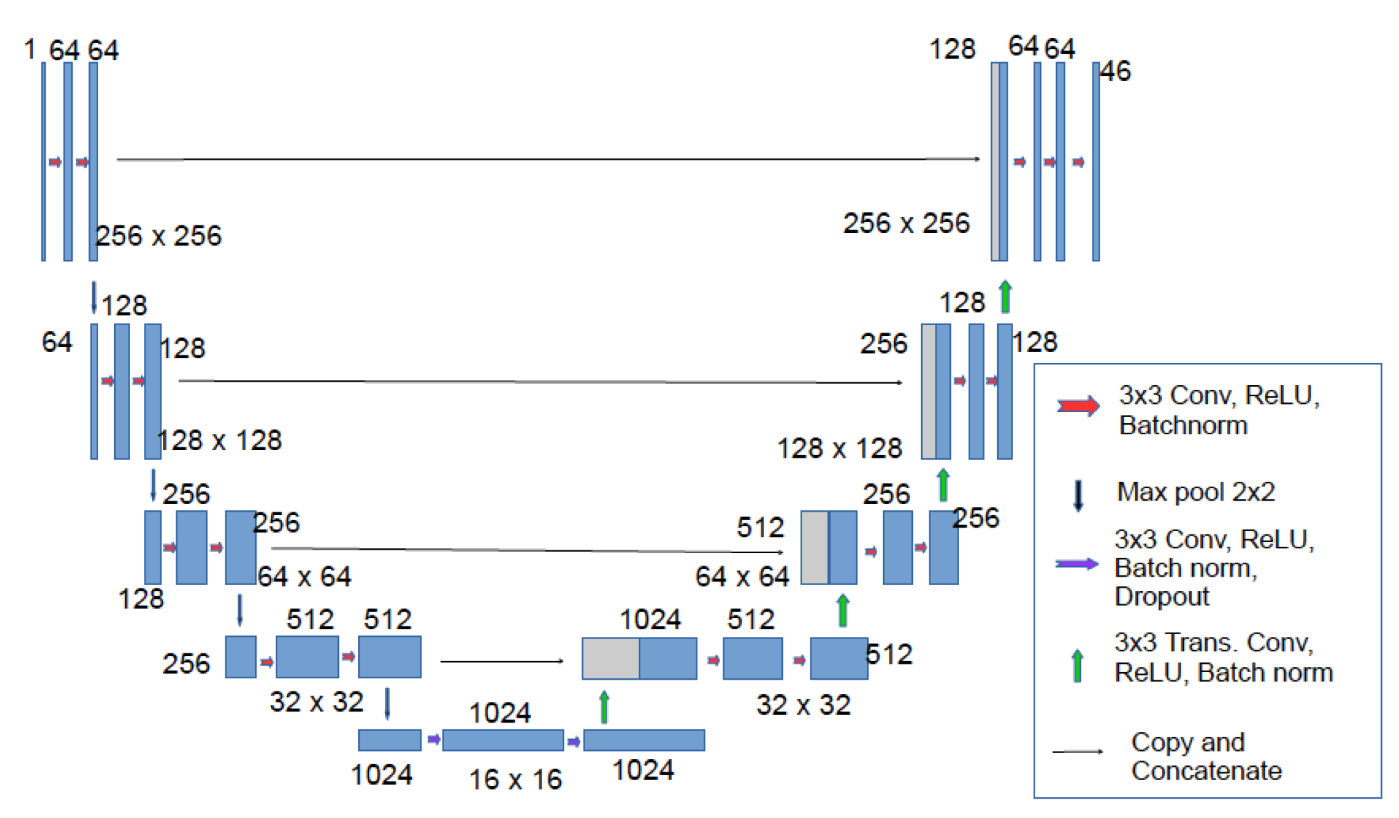
The contraction part is made up of a number of contraction pieces. Each block must take a single input, apply two convolution layers and then pool to an amount of maximum. The number of kernels or feature mappings is doubled after each block to allow a design to learn the complex pattern in its entirety. The lower layer is a bridge between the contraction and extension layers. After two CNN layers, a up convolution layer is used.
When processing dataset, the up-sampling layer is added after each block’s two CNN layers. In addition, the number of mapping elements used in a convolution layer shall be reduced by half following each block to ensure balance. The input is also supplemented with feature maps derived from a corresponding contraction layer every time. As there are same number of blocks for contraction and expansion, which ensure that the qualities that a picture gains as it gets smaller are also used to reconstruct it in its ultimate form. After that, output mapping is handled by applying a second CNN layer with the same number of feature maps.
U-Net uses a distinct way of weighting the losses for each pixel, assigning more weight to the edges of divided objects. Using this loss weighting method, the U-Net model was able to segment cells on biomedical images in a continuous manner, which allowed for easy identification of individual cells within binary segmentation maps. Initially, the final image undergoes a softmax transformation on a per-pixel basis, and then a loss function that measures the difference between predicted and actual values is applied. This allows us to classify each image into a specific category. It is necessary for each pixel to be assigned to a particular group, even during segmentation, which can be accomplished by ensuring that they do. As a result, a segmentation issue is changed into a multiclass classification problem.
In the proposed technique, this model is used with the bit of change in parameters like Exponential Linear Unit (ELU) as activation function in input layers etc., which is also very similar to ReLU, except for negative inputs [52]. This function is basically designed to address the vanishing gradient problem that can occur during training with the ReLU function. When the ReLU function is used, the output of the function is 0 for negative inputs, which can cause the gradient of the function to be 0 as well. This can result in slower training and a higher risk of the network getting stuck in a local minimum. The ELU allows negative inputs to have a non-zero output. This helps to prevent the gradient from becoming 0 and ensures that the network can continue to learn from negative inputs. As opposed to ReLU, which smooths abruptly, ELU smooths down gradually until its output equals.
The mathematical formula for the ELU is:
Where x is the input to the activation function, and is a hyper-parameter that determines the value of the function for negative inputs and it is typically set to a small positive value such as . This ensures that the function is close to 0 for negative inputs, not exactly 0, so the gradient is non-zero.
When using ELU in a U-Net architecture, it can help improve the model’s performance by addressing the vanishing gradient problem, which can occur during training. Vanishing gradient is situation when gradient becomes very small as they propagate backward through a deep neural network, making it difficult to update the weights. By using ELU, this situation can be mitigated to some extent and the model can produce more accurate segmentation while also reducing the training time and improving the convergence rate.
During training to evaluate the performance of U-Net between the predicted segmentation mask and the ground truth mask, Dice Similarity Coefficient [53] is used. Dice Similarity is sensitive to small variations in the segmentation masks, which is important in critical applications like medical imaging. Dice coefficient is usually computed for each class separately and then averaged over all classes to obtain a final score. A dice coefficient value of 1 indicates perfect overlap between the predicted and ground truth masks, while a value of 0 indicates no overlap. It is defined as the ratio of the intersection of the two masks to the total number of pixels in the two masks, specifically:
Where A and B are the two binary masks.
After training model on the images and their masks, it predicts mask for the test dataset. These predicted masks will then be used for angle calculation.
2.7. Angle Calculation
To calculate the angle on the predicted masks, custom code is written which operates in the manner of finding the slope from the masked spine and calculating the degree of angles for every bend of each image. In total, three angles (for each bend) are being calculated for each image. These predicted angles are then compared with the given angles for result analysis.
2.8. Result Analysis
RMSE is used as a basic measure to analyze the results. RMSE is a commonly used metric for evaluating the accuracy of a prediction or model. It represents the square root of the average squared difference between the actual and predicted values. The lower the RMSE, the better the accuracy of the prediction or model.
The formula for RMSE can be expressed as:
Where is the actual value of the data point, is the predicted value of the data point, and n is the total number of data points.
For visualization of results, ground truths and prediction were plotted using the simple plots, scatter plots and Q-Q plots. In a scatter plot, each point on the plot represents a pair of values, one from each dataset and can be represented as .
Where and are the values from the two datasets. The scatter plot shows the distribution of these points on a two-dimensional coordinate system, with the x-axis representing one dataset and the y-axis representing the other.
In a scatter plot, the distribution of points can reveal important information about the relationship between the two datasets. For example, if the points are tightly clustered around a line, this suggests a strong linear relationship between the two datasets. If the points are scattered randomly, this suggests no significant relationship between the two datasets.
The Quantile-Quantile (Q-Q) plot is a graphical tool for comparing the distribution of a sample of dataset to a theoretical distribution, such as the normal distribution. The mathematics behind the Q-Q plot involves plotting the quantiles of the sample dataset against the quantiles of the theoretical distribution. It can be understood as: .
Where are the ordered values of the sample data, and are the corresponding quantiles of the theoretical distribution.
The Q-Q plot shows how well the sample data fits the theoretical distribution. If the sample data is normally distributed, the points on the Q-Q plot will approximately fall on a straight line. If the sample data is not normally distributed, the points on the Q-Q plot will deviate from a straight line.
To construct a Q-Q plot, the sample data is first sorted in ascending order. The corresponding quantiles of the theoretical distribution are then calculated using a formula or a lookup table. The ordered values of the sample data are plotted on the x-axis, and the corresponding quantiles of the theoretical distribution are plotted on the y-axis. The resulting plot shows the relationship between the sample data and the theoretical distribution. A sample of Q-Q plot is shown in Figure 13.
3. Experimental Setup
The dataset used for implementation is acquired from MICCAI Challenge Board, 609 spinal anterior-posterior X-ray images. It consists of 481 training images and 128 testing images. Input images vary in size from to . For every training and testing image labels and angles are provided in CSV format. Label of a particular image contain the landmarks of vertebrates present in that image. Angles contain the Cobbâs angles of every imageâs scoliotic spine.
For an image, three angles are given in respect to right, left and right bend which are interpreted as ground truth in development. The angles are calculated in the same manner while making prediction.
Taking the bench mark dataset into consideration, first of all it is gone through the process of contrast improvement (pre-processing) with the parameter values as clip limit of and tile grid size of 8. After that final pre-processed image is obtained. An instance of pre-processed image is shown in Figure 14.
After contrast improvement, Gaussian noise is added in of total dataset (481 samples), and in the next 10 percent, Salt-and-Pepper noise is added. Gaussian and Impulse noise additive image in comparison to the pre-processed image can be seen in Figure 15.
For the next slab of 10 percent, intelligent cropping is performed which set the upper crop limit to ratio and the lower limit to of the original image’s height and width, making the spine portion in center, presented in Figure 16.
To identify the spine portion, the land marking is performed by reading the image into arrays and converting theses array into two columns of x and y coordinates leading to the transformation into pixel values. Plot of these pixel values highlight the spine area. The red highlighted dash lines around the spine in Figure 17 refers to the landmarks of the spine.
On these pixel values, continuous boundary is drawn and contouring is done using python libraries which in result gives the binary mask of image. Figure 18 reveals the mask of the left side place image on the right side.
These generated masks and their input images are then flipped and rotated to 10 degrees with respect to center to increase the sample size from 481 to 1433 instances. In Figure 19, flipped and 10-degree rotated version of image is displayed.
All the instances of images and masks are then serialized to pickles which is then fed to U-Net architecture for segmentation. The model is trained using the cross-entropy loss function, which is commonly used for image segmentation tasks. ELU and sigmoid is used as activation functions in input and output layers respectively, which has been shown to be effective in deep learning models by addressing the vanishing gradient problem.
During training, we used the dice coefficient as performance metric to evaluate the accuracy of the segmentation. The dice coefficient measures the overlap between the predicted segmentation mask and the ground truth mask, with a value of 1 indicating a perfect match. Table 2 summarizes the hyper-parameters used in U-Net model.
As the Adam optimizer is used, so by default the learning rate of is chosen. The batch size of 64 was selected to ensure efficient memory usage and faster convergence during training. The increasing number of filters are used in encoder pathway to capture more complex features () while decreasing the number of filters in decoder pathway to prevent over-fitting (). A range dropout rate is applied to prevent over-fitting. Finally, a 3 x 3 kernel size was used to capture local features and ensure that the model can capture fine details in the images and the model is trained for 50 epochs over the training dataset which was randomly split into training and validation sets, with 15% of the dataset reserved for validation. Training accuracy of model is observed to % and validation accuracy to %.
The weights of the model are saved using the checker point as the training time is way longer. So the model’s current state is being snapped.
By loading the trained model, predictions are made on the testing dataset which gives masks for 128 testing samples. On these predicted masks, angle is calculated by finding the maximum and minimum slope found using the landmarks. First angle is calculated as a difference of maximum and minimum slope and converting it to degrees. The second and third angle is estimated with the difference of maximum and minimum in the upper portion of maximum slope found on the first level and in lower portion respectively. In result, three angles are measured for one sample.
4. Results & Discussion
The performance of the proposed technique is evaluated on MICCAI dataset of 609 spinal anterior-posterior 1433 X-ray images, with a validation split of . The RMSE and MAE is used as the evaluation metric to measure the accuracy of the model. The U-Net model achieved an RMSE of , indicating that the average difference between predicted and ground truth values is relatively low. While the MAE approached to . For all the first angles of both the ground truth and prediction are plotted in Figure 20, which clearly shows that there are no discrepancies and predicted values closely matches with the ground truth values.
Similarly, Figure 21 and Figure 22 shows the plots drawn for angle 2 and 3 respectively, which depicts that presented legends of both the predicted and ground truth are closely coupled.
These results were obtained till 50 epochs. Performance plot in Figure 23 provides valuable insights into the accuracy progression of the U-Net model over a specified number of epochs. In this proposed technique, U-Net model is trained for 20 epochs, resulting in a final accuracy of starting from an initial accuracy of . To explore the potential for further improvements, we extended the training to 50 epochs, where we achieved an accuracy of range .
While the accuracy improvement within the initial 20 epochs is commendable, it is essential to consider potential challenges associated with a limited number of epochs when training complex models such as U-Net. One problem that arises is the insufficient time for the model to fully converge and capture intricate patterns in the dataset. This limitation may lead to sub-optimal accuracy levels or accuracy plateaus before reaching the model’s maximum potential. Extending it to 50, allowed the U-Net model to further refine its representations, optimize its parameters, and improve its accuracy. The observed accuracy of within the 50 epochs demonstrates the model’s ability to learn complex image segmentation tasks effectively. By providing more time for the model to explore the dataset and refine its predictions, we enable it to capture finer details and enhance its segmentation performance.
To further analyze the performance of the model, scatter plots were used to visualize the predicted segmentation masks against the ground truth masks. Figure 24 shows the scatter plot between the predicted and ground truth segmentation masks. The plot indicates that the predicted masks closely follow the ground truth masks, with only a few outliers.
In addition, a Q-Q plot is created to visually assess the similarity between the distribution of the ground truth values and the distribution of the predicted values. The points on the Q-Q plot fell along a straight line, suggesting that the predicted values were similar to the ground truth values in Figure 25. These results indicate that the U-Net model performed well on the dataset and was able to accurately capture the underlying patterns in the dataset.
Overall, the results demonstrate that the use of deep learning model, such as the U-Net in addition to some techniques like the use of custom code, noise addition etc. has shown promise for accurately measuring the Cobb’s angle in scoliosis patients. By using deep learning techniques, the proposed technique provides an automated and objective approach to measuring the Cobbâs angle, which can reduce the variability and subjectivity associated with manual measurements. One significant advantage of the proposed technique is the elimination of the manual cropping step which is very crucial for [30] model performance. The achieved MAE of indicates a high level of accuracy in estimating the Cobb’s angle, demonstrating the efficiency of the proposed technique building upon in comparison to the foundation laid by a technique based on cascaded neural networks [30]. Comprehensively, the proposed technique provides an accurate and efficient approach to measuring the Cobb’s angle of scoliosis, which could have important clinical implications for the diagnosis and treatment of scoliosis patients over other approaches and comparison with some of the researches can be seen in Table 3.
While this proposed technique explains the potential of deep learning models for accurately measuring the Cobb’s angle of scoliosis, there is still room for improvement. Firstly, there is a lack of ground truth masks for the testing dataset, which hinders the ability to validate the correctness of the results accurately. Ground truth masks provide precise annotations of scoliosis regions, allowing for reliable comparisons with predicted outcomes. Efforts should be made to acquire or create ground truth masks to enhance the evaluation process. Additionally, the evaluation dataset used in this proposed technique have limitations, including a small sample size, limited diversity in terms of age or severity of scoliosis, and inadequate representation of different curve types. These limitations impact the generalizability and robustness of the proposed technique. Further validation and clinical trials are necessary to ensure the effectiveness of the proposed technique across diverse dataset and real-world scenarios. Collaborations with healthcare professionals and integration of additional clinical dataset can provide valuable insights for refining and fine-tuning of the proposed technique.
5. Conclusions & Future Work
This research builds upon the existing work by incorporating image enhancement, deep learning techniques and a customized algorithm for landmark estimation, segmentation and angle measurement, resulting in notable improvements in scoliosis evaluation. The accuracy rate signifies a strong correlation between the automated measurement of proposed technique and manual assessments performed by experts, indicating the reliability and precision of this method.
Through the optimization of the process and elimination of manual intervention, a dual benefit of reducing human errors while also improving the efficiency and scalability of the proposed technique is achieved. This automation can potentially expedite the diagnosis and treatment of scoliosis, allowing healthcare professionals to allocate their time and resources more effectively.
The combination of deep learning techniques, accurate landmark estimation, and segmentation has enabled us to develop an automated system that can consistently and objectively measure the Cobb’s angle with high accuracy. This advancement has the potential to improve the quality of scoliosis diagnosis, optimize treatment planning, and enhance patient outcomes.
Future work could also explore ways to further improve the performance of the proposed technique, such as using larger datasets, incorporating additional features or modalities, or exploring alternative deep learning architectures. The clinical implications of using the proposed technique for diagnosis of scoliosis and it’s treatment can also be investigated.
Conflicts of Interest
There is no conflict of interest between the authors.
Availability of Data
The datasets used in this research are bench mark datasets, available publicly.
Code Availability
Code can be provided on request.
Author Contributions
All authors worked equally.
References
- Negrini, S.; Donzelli, S.; Aulisa, A.G.; Czaprowski, D.; Schreiber, S.; de Mauroy, J.C.; Diers, H.; Grivas, T.B.; Knott, P.; Kotwicki, T.; others. 2016 SOSORT guidelines: orthopaedic and rehabilitation treatment of idiopathic scoliosis during growth. Scoliosis and spinal disorders 2018, 13, 1–48. [Google Scholar]
- Asher, M.A.; Burton, D.C. Adolescent idiopathic scoliosis: natural history and long term treatment effects. Scoliosis 2006, 1, 1–10. [Google Scholar] [CrossRef]
- Khan, M.; Naseer, A.; Wali, A.; Tamoor, M. A Roman Urdu Corpus for sentiment analysis. The Computer Journal, 2024; bxae052. [Google Scholar]
- Gorman, K.F.; Julien, C.; Moreau, A. The genetic epidemiology of idiopathic scoliosis. European Spine Journal 2012, 21, 1905–1919. [Google Scholar] [CrossRef] [PubMed]
- Tamoor, M.; Osama, S.; Younas, I.; Asif, S. Comparison of different multi objective evolutionary algorithms for bug localization. International Conference on Advances on Applied Cognitive ComputingâACC, 2018.
- Tamoor, M.; Gul, H.; Qaiser, H.; Ali, A. An optimal formulation of feature weight allocation for CBR using machine learning techniques. 2015 SAI Intelligent Systems Conference (IntelliSys). IEEE, 2015, pp. 61–67.
- Tamoor, M.; Naseer, A.; Khan, A.; Zafar, K. Skin lesion segmentation using an ensemble of different image processing methods. Diagnostics 2023, 13, 2684. [Google Scholar] [CrossRef] [PubMed]
- Tan, Z.; Yang, K.; Sun, Y.; Wu, B.; Tao, H.; Hu, Y.; Zhang, J. An automatic scoliosis diagnosis and measurement system based on deep learning. 2018 IEEE International Conference on Robotics and Biomimetics (ROBIO). IEEE, 2018, pp. 439–443.
- Nawaz, M.; Adnan, A.; Tariq, U.; Salman, F.; Asjad, R.; Tamoor, M. Automated career counseling system for students using cbr and j48. Journal of Applied Environmental and Biological Sciences 2015, 4, 113–120. [Google Scholar]
- Reamy, B.V.; Slakey, J.B. Adolescent idiopathic scoliosis: review and current concepts. American family physician 2001, 64, 111–117. [Google Scholar] [PubMed]
- Wali, A.; Ahmad, M.; Naseer, A.; Tamoor, M.; Gilani, S. Stynmedgan: medical images augmentation using a new GAN model for improved diagnosis of diseases. Journal of Intelligent & Fuzzy Systems 2023, 44, 10027–10044. [Google Scholar]
- Lonstein, J.E.; Carlson, J. The prediction of curve progression in untreated idiopathic scoliosis during growth. JBJS 1984, 66, 1061–1071. [Google Scholar] [CrossRef]
- Saleem, M.A.; Tamoor, M.; Asif, S. An efficient method for gender classification using hybrid CBR. 2016 Future Technologies Conference (FTC). IEEE, 2016, pp. 116–120.
- Malik, Y.S.; Tamoor, M.; Naseer, A.; Wali, A.; Khan, A. Applying an adaptive Otsu-based initialization algorithm to optimize active contour models for skin lesion segmentation. Journal of X-Ray Science and Technology 2022, 30, 1169–1184. [Google Scholar] [CrossRef]
- Naseer, A.; Tamoor, M.; Khan, A.; Akram, D.; Javaid, Z. Occupancy detection via thermal sensors for energy consumption reduction. Multimedia Tools and Applications 2024, 83, 4915–4928. [Google Scholar] [CrossRef]
- Tamoor, M.; Younas, I. Automatic segmentation of medical images using a novel Harris Hawk optimization method and an active contour model. Journal of X-ray Science and Technology 2021, 29, 721–739. [Google Scholar] [CrossRef]
- Chughtai, I.T.; Naseer, A.; Tamoor, M.; Asif, S.; Jabbar, M.; Shahid, R. Content-based image retrieval via transfer learning. Journal of Intelligent & Fuzzy Systems 2023, 44, 8193–8218. [Google Scholar]
- Raza, N.; Naseer, A.; Tamoor, M.; Zafar, K. Alzheimer disease classification through transfer learning approach. Diagnostics 2023, 13, 801. [Google Scholar] [CrossRef]
- Naseer, A.; Tamoor, M.; Azhar, A. Computer-aided COVID-19 diagnosis and a comparison of deep learners using augmented CXRs. Journal of X-ray Science and Technology 2022, 30, 89–109. [Google Scholar] [CrossRef] [PubMed]
- Kuklo, T.R.; Potter, B.K.; Polly Jr, D.W.; OâBrien, M.F.; Schroeder, T.M.; Lenke, L.G. Reliability analysis for manual adolescent idiopathic scoliosis measurements. Spine 2005, 30, 444–454. [Google Scholar] [CrossRef] [PubMed]
- Negrini, S.; Minozzi, S.; Bettany-Saltikov, J.; Chockalingam, N.; Grivas, T.B.; Kotwicki, T.; Maruyama, T.; Romano, M.; Zaina, F. Braces for idiopathic scoliosis in adolescents. Cochrane Database of Systematic Reviews 2015. [Google Scholar] [CrossRef]
- Nault, M.L.; Mac-Thiong, J.M.; Roy-Beaudry, M.; Turgeon, I.; Deguise, J.; Labelle, H.; Parent, S. Three-dimensional spinal morphology can differentiate between progressive and nonprogressive patients with adolescent idiopathic scoliosis at the initial presentation: a prospective study. Spine 2014, 39, E601. [Google Scholar] [CrossRef]
- M. Clinic. Scoliosis. [Online]. Available: https://www.mayoclinic.org/diseases-conditions/scoliosis/symptoms-causes/syc-20350716.
- Davids, J.R.; Chamberlin, E.; Blackhurst, D.W. Indications for magnetic resonance imaging in presumed adolescent idiopathic scoliosis. JBJS 2004, 86, 2187–2195. [Google Scholar] [CrossRef]
- Larson, A.N.; Fletcher, N.D.; Daniel, C.; Richards, B.S. Lumbar curve is stable after selective thoracic fusion for adolescent idiopathic scoliosis: a 20-year follow-up. Spine 2012, 37, 833–839. [Google Scholar] [CrossRef] [PubMed]
- Physiopedia. Cobbâs angle. [Online]. Available: https://www.physio-pedia.com/CobbAngle.
- Sun, Y.; Xing, Y.; Zhao, Z.; Meng, X.; Xu, G.; Hai, Y. Comparison of manual versus automated measurement of Cobb angle in idiopathic scoliosis based on a deep learning keypoint detection technology. European Spine Journal 2022, 31, 1969–1978. [Google Scholar] [CrossRef]
- Jin, C.; Wang, S.; Yang, G.; Li, E.; Liang, Z. A Review of the Methods on Cobb Angle Measurements for Spinal Curvature. Sensors 2022, 22, 3258. [Google Scholar] [CrossRef] [PubMed]
- Maaliw, R.R.; Susa, J.A.B.; Alon, A.S.; Lagman, A.C.; Ambat, S.C.; Garcia, M.B.; Piad, K.C.; Fernando Raguro, M.C. A Deep Learning Approach for Automatic Scoliosis Cobb Angle Identification. 2022 IEEE World AI IoT Congress (AIIoT), 2022, pp. 111–117. [CrossRef]
- Dubost, F.; Collery, B.; Renaudier, A.; Roc, A.; Posocco, N.; Niessen, W.; de Bruijne, M. Automated estimation of the spinal curvature via spine centerline extraction with ensembles of cascaded neural networks. International Workshop and Challenge on Computational Methods and Clinical Applications for Spine Imaging. Springer, 2020, pp. 88–94.
- Vyas, D.; Ganesan, A.; Meel, P. Computation and Prediction Of Cobb’s Angle Using Machine Learning Models. 2022 2nd International Conference on Intelligent Technologies (CONIT). IEEE, 2022, pp. 1–6.
- Khanal, B.; Dahal, L.; Adhikari, P.; Khanal, B. Automatic cobb angle detection using vertebra detector and vertebra corners regression. International Workshop and Challenge on Computational Methods and Clinical Applications for Spine Imaging. Springer, 2020, pp. 81–87.
- Fu, X.; Yang, G.; Zhang, K.; Xu, N.; Wu, J. An automated estimator for Cobb angle measurement using multi-task networks. Neural Computing and Applications 2021, 33, 4755–4761. [Google Scholar] [CrossRef]
- Caesarendra, W.; Rahmaniar, W.; Mathew, J.; Thien, A. Automated Cobb Angle Measurement for Adolescent Idiopathic Scoliosis Using Convolutional Neural Network. Diagnostics 2022, 12, 396. [Google Scholar] [CrossRef]
- Wong, J.; Reformat, M.; Parent, E.; Lou, E. Convolutional neural network to segment laminae on 3D ultrasound spinal images to assist cobb angle measurement. Annals of Biomedical Engineering 2022, 50, 401–412. [Google Scholar] [CrossRef] [PubMed]
- Cui, J.L.; Gao, D.D.; Shen, S.J.; Wang, L.Z.; Zhao, Y. Cobb Angle Measurement Method of Scoliosis Based on U-net Network. Research Square 2021. [Google Scholar]
- Sun, H.; Zhen, X.; Bailey, C.; Rasoulinejad, P.; Yin, Y.; Li, S. Direct estimation of spinal cobb angles by structured multi-output regression. International conference on information processing in medical imaging. Springer, 2017, pp. 529–540.
- Garcia-Cano, E.; Cosío, F.A.; Duong, L.; Bellefleur, C.; Roy-Beaudry, M.; Joncas, J.; Parent, S.; Labelle, H. Prediction of spinal curve progression in adolescent idiopathic scoliosis using random forest regression. Computers in biology and medicine 2018, 103, 34–43. [Google Scholar] [CrossRef]
- Alukaev, D.; Kiselev, S.; Mustafaev, T.; Ainur, A.; Ibragimov, B.; Vrtovec, T. A deep learning framework for vertebral morphometry and Cobb angle measurement with external validation. European Spine Journal, 2022; 1–10. [Google Scholar]
- Makhdoomi, N.A.; Gunawan, T.S.; Idris, N.H.; Khalifa, O.O.; Karupiah, R.K.; Bramantoro, A.; Rahman, F.D.A.; Zakaria, Z. Development of Scoliotic Spine Severity Detection using Deep Learning Algorithms. 2022 IEEE 12th Annual Computing and Communication Workshop and Conference (CCWC). IEEE, 2022, pp. 0574–0579.
- Huang, X.; Luo, M.; Liu, L.; Wu, D.; You, X.; Deng, Z.; Xiu, P.; Yang, X.; Zhou, C.; Feng, G. ; others. The Comparison of Convolutional Neural Networks and the Manual Measurement of Cobb Angle in Adolescent Idiopathic Scoliosis. Global Spine Journal, 2022; 21925682221098672. [Google Scholar]
- Wang, Y.; Huang, L.; Wu, M.; Liu, S.; Jiao, J.; Bai, T. Multi-input adaptive neural network for automatic detection of cervical vertebral landmarks on X-rays. Computers in biology and medicine 2022, 146, 105576. [Google Scholar] [CrossRef] [PubMed]
- Magnide, E.; Tchaha, G.W.; Joncas, J.; Bellefleur, C.; Barchi, S.; Roy-Beaudry, M.; Parent, S.; Grimard, G.; Labelle, H.; Duong, L. Automatic bone maturity grading from EOS radiographs in Adolescent Idiopathic Scoliosis. Computers in Biology and Medicine 2021, 136, 104681. [Google Scholar] [CrossRef]
- Zuiderveld, K. Contrast limited adaptive histogram equalization. Graphics gems, 1994; 474–485. [Google Scholar]
- Pizer, S.M.; Amburn, E.P.; Austin, J.D.; Cromartie, R.; Geselowitz, A.; Greer, T.; ter Haar Romeny, B.; Zimmerman, J.B.; Zuiderveld, K. Adaptive histogram equalization and its variations. Computer vision, graphics, and image processing 1987, 39, 355–368. [Google Scholar] [CrossRef]
- Shorten, C.; Khoshgoftaar, T.M. A survey on image data augmentation for deep learning. Journal of big data 2019, 6, 1–48. [Google Scholar] [CrossRef]
- Cheng, X.; Hao, Y.; Xu, J.; Xu, B. LISNN: Improving spiking neural networks with lateral interactions for robust object recognition. IJCAI. Yokohama, 2020, pp. 1519–1525.
- Goyal, B.; Agrawal, S.; Sohi, B. Noise issues prevailing in various types of medical images. Biomedical & Pharmacology Journal 2018, 11, 1227. [Google Scholar]
- Jiang, Y.; Wang, H.; Cai, Y.; Fu, B. Salt and Pepper Noise Removal Method Based on the Edge-adaptive Total Variation Model. Frontiers in Applied Mathematics and Statistics 2022, 8. [Google Scholar] [CrossRef]
- Ronneberger, O.; Fischer, P.; Brox, T. U-net: Convolutional networks for biomedical image segmentation. Medical Image Computing and Computer-Assisted Intervention–MICCAI 2015: 18th International Conference, Munich, Germany, October 5-9, 2015, Proceedings, Part III 18. Springer, 2015, pp. 234–241.
- C. V. Hegde. Brain segmentation using deep learning poster. [Online]. Available: https://cds.nyu.edu/brainsegmentation-poster/.
- Clevert, D.A.; Unterthiner, T.; Hochreiter, S. Fast and accurate deep network learning by exponential linear units (elus). arXiv preprint, 2015; arXiv:1511.07289 2015. [Google Scholar]
- Milletari, F.; Navab, N.; Ahmadi, S.A. V-net: Fully convolutional neural networks for volumetric medical image segmentation. 2016 fourth international conference on 3D vision (3DV). IEEE, 2016, pp. 565–571.
Figure 1.
Scoliotic View of a Normal Spine [23].
Figure 1.
Scoliotic View of a Normal Spine [23].
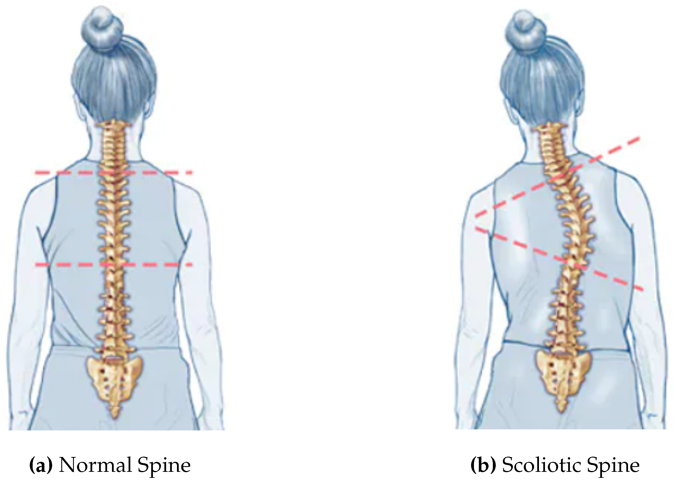
Figure 2.
Measurement of Cobb’s angle [26].
Figure 2.
Measurement of Cobb’s angle [26].
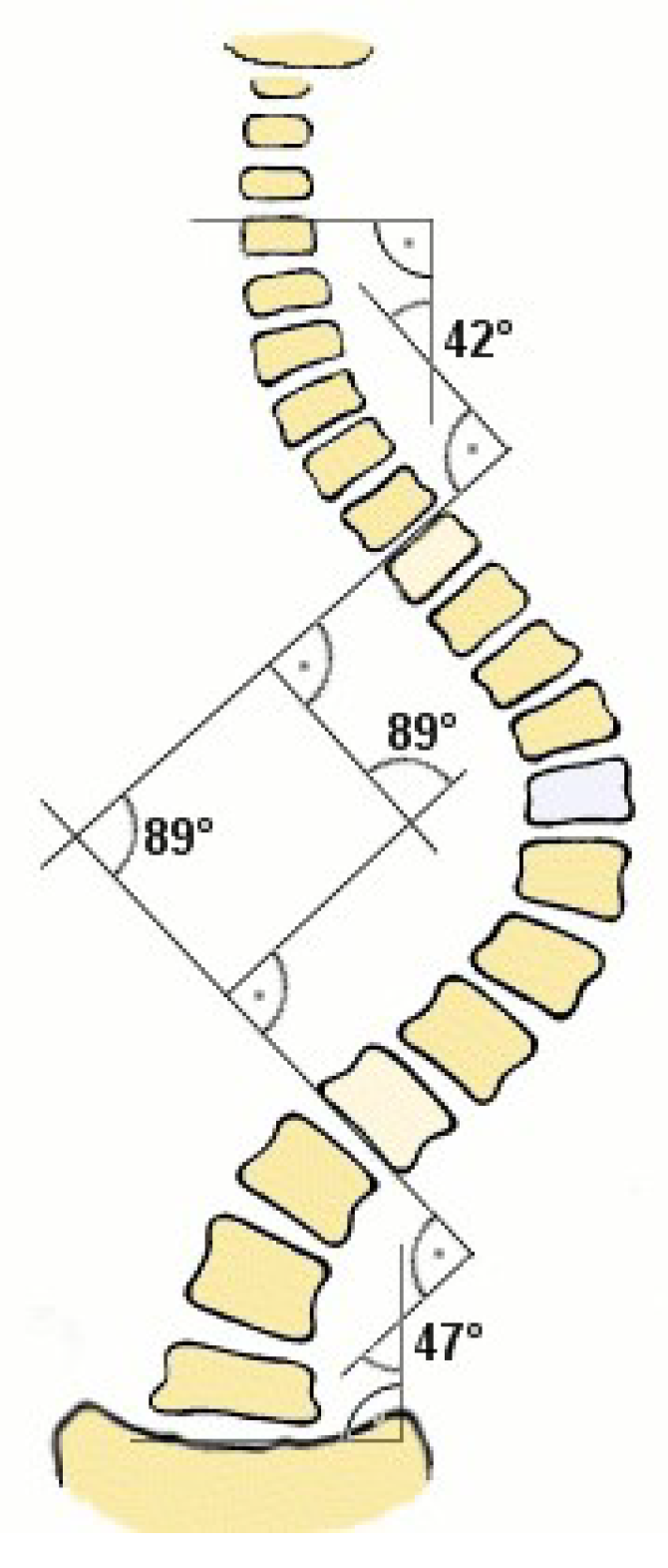
Figure 3.
High Level Architecture.
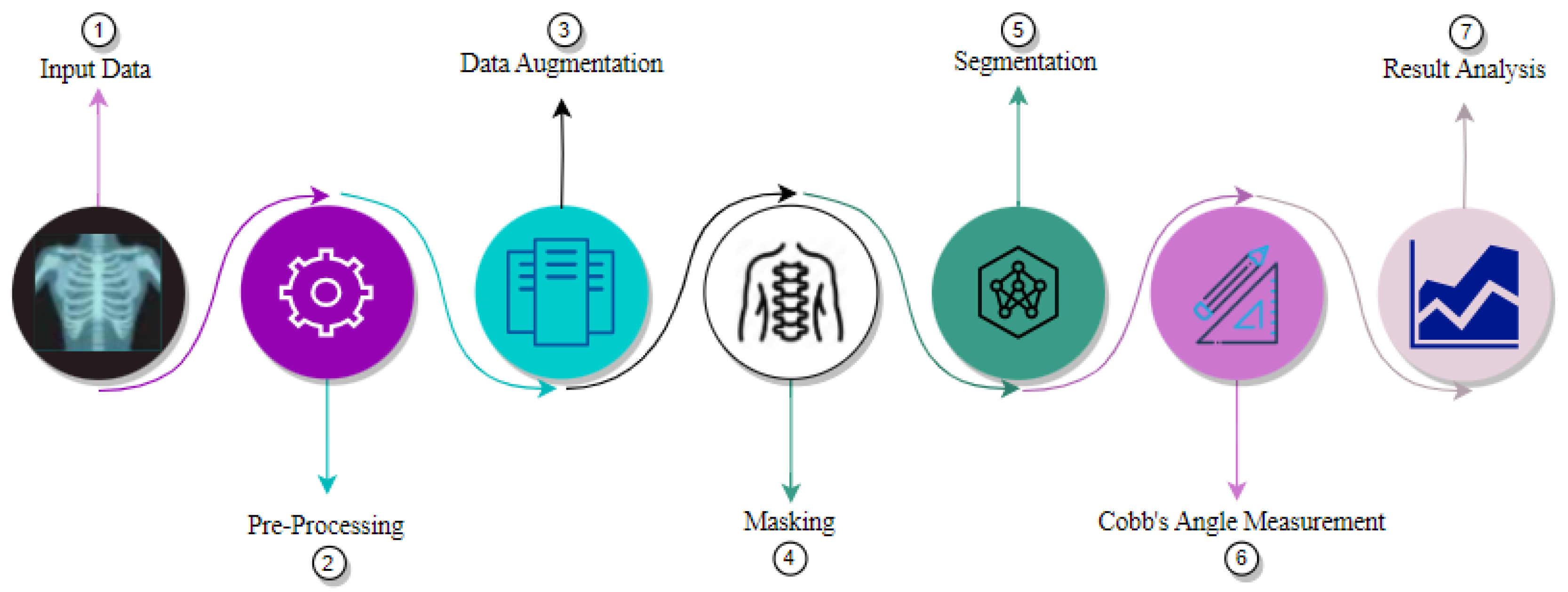
Figure 4.
In-depth Architecture.

Figure 5.
Original vs Pre-processed Image.
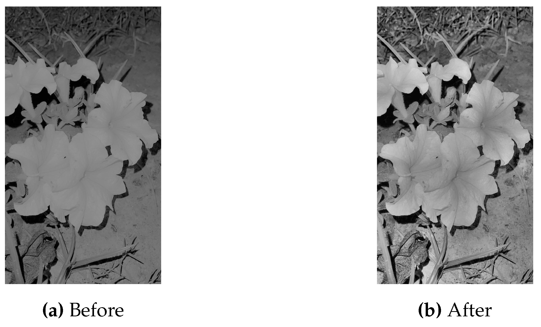
Figure 6.
Image with Gaussian Noise.
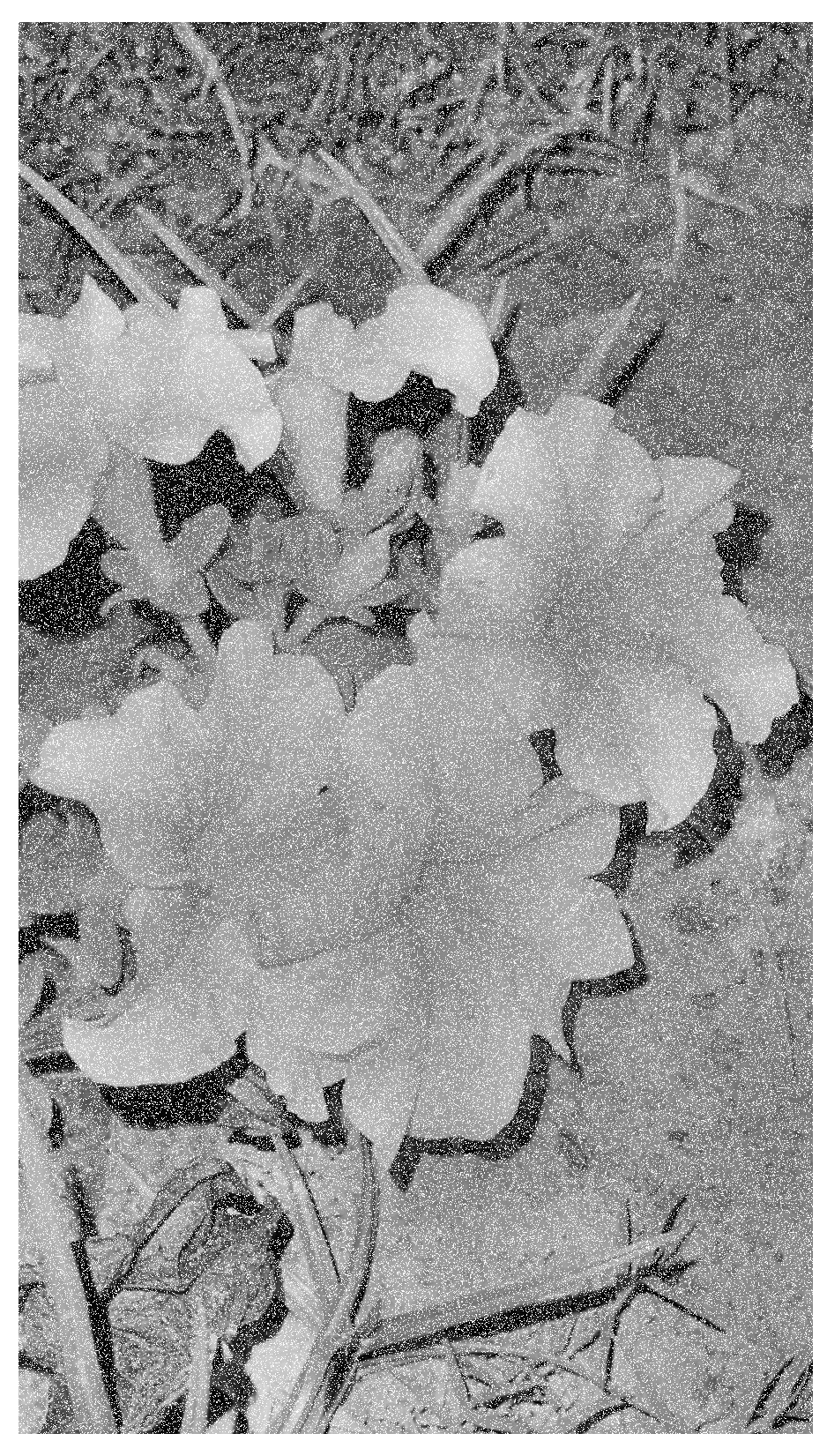
Figure 7.
Image with Salt-and-Pepper Noise.
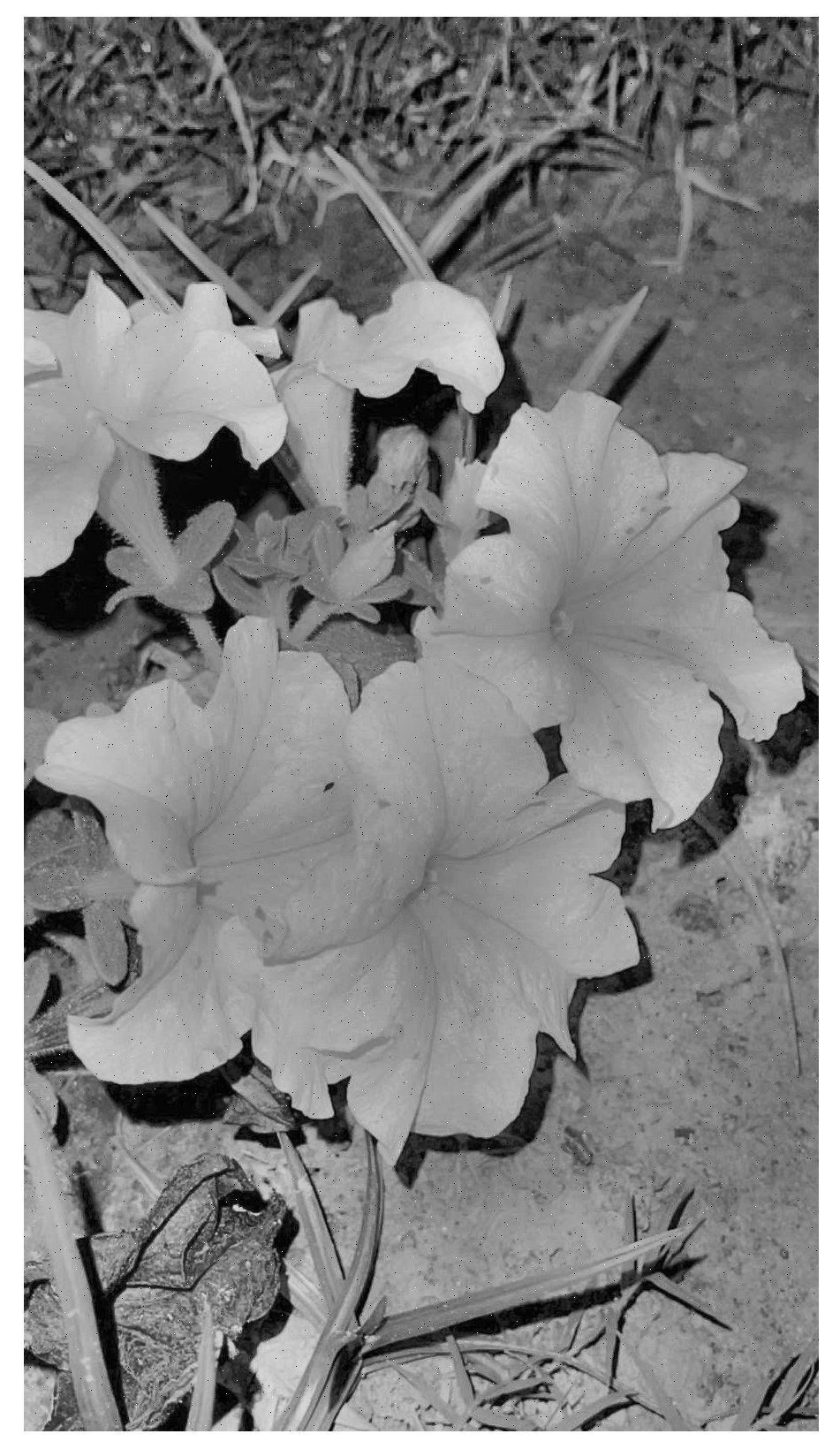
Figure 8.
Intelligently Cropped Image.
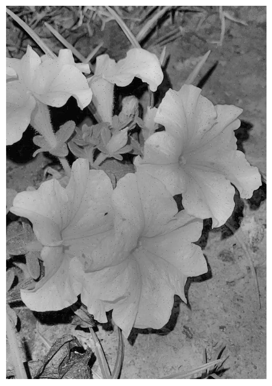
Figure 9.
Flipped vs Rotated versions of the Original Image.
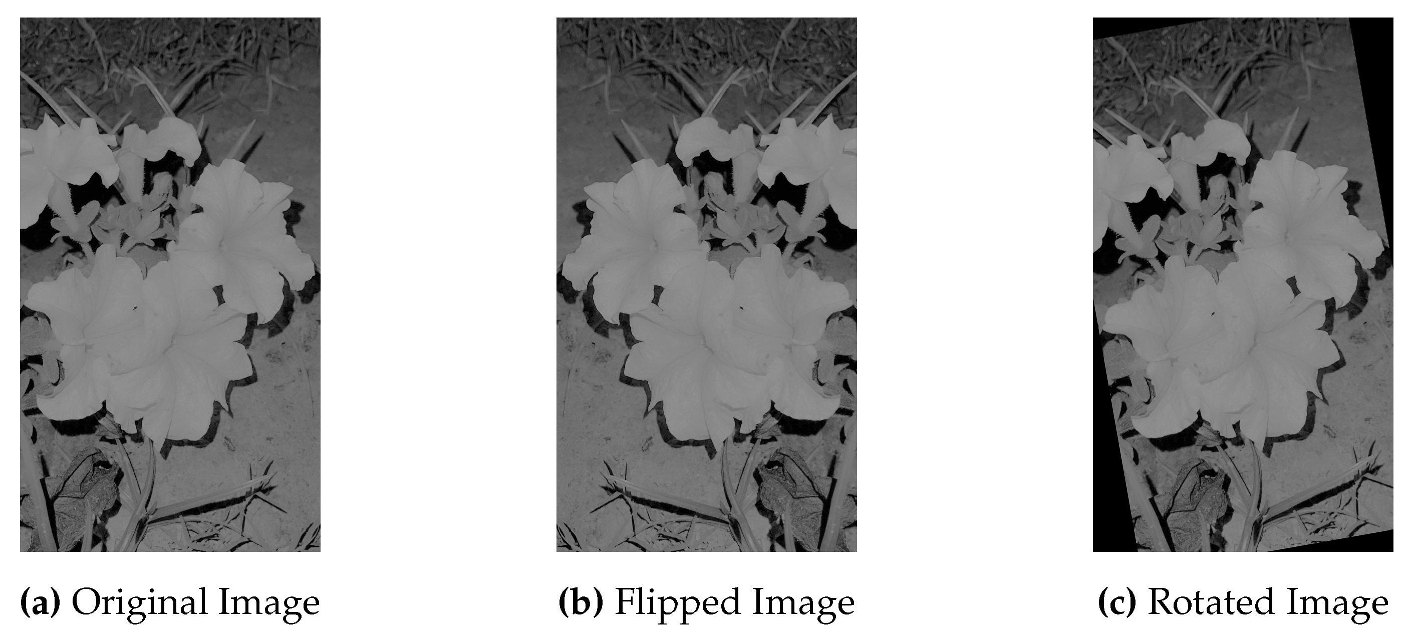
Figure 10.
Visualization of Landmarks on Original Images.
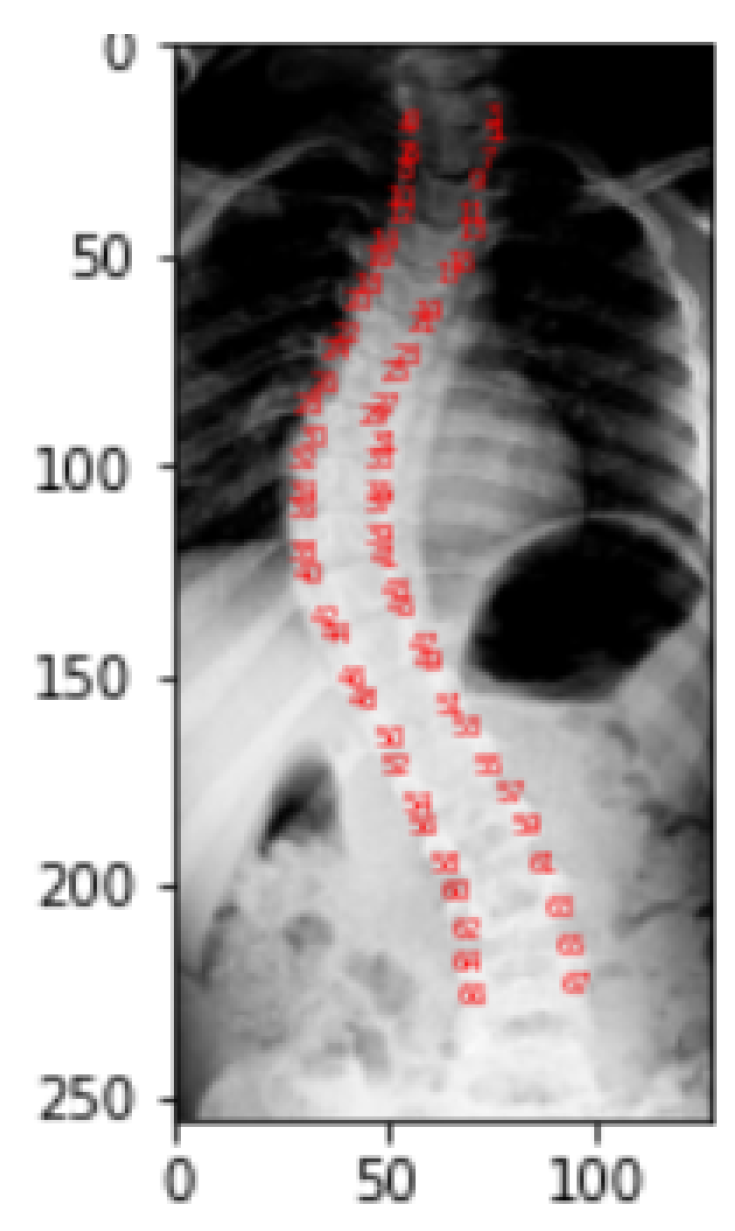
Figure 11.
Mask of the Original Image.
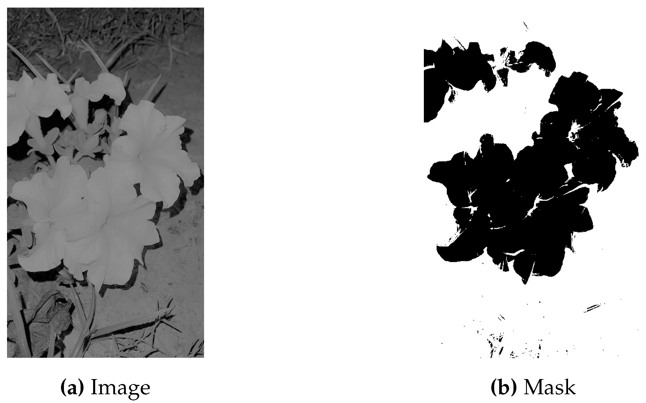
Figure 13.
Q-Q Plot.
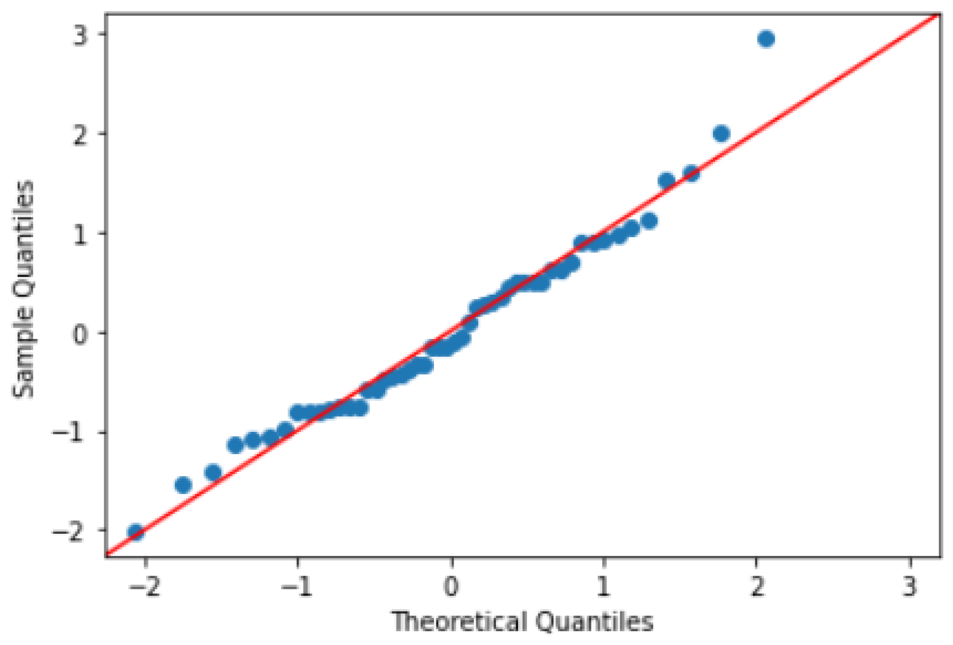
Figure 14.
Before and After Pre-processing.
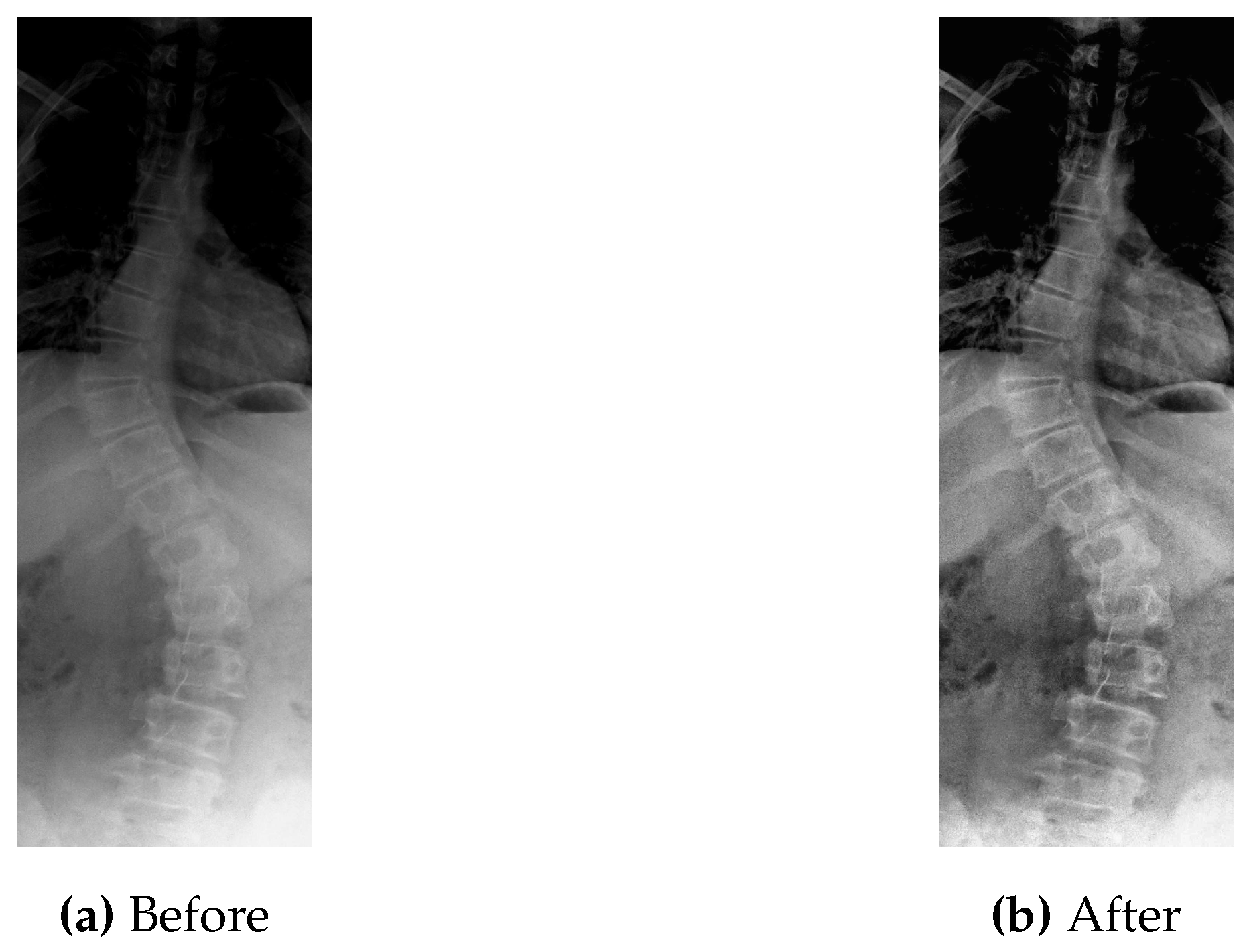
Figure 15.
Pre-processed Image with Gaussian and Impulse Noise.
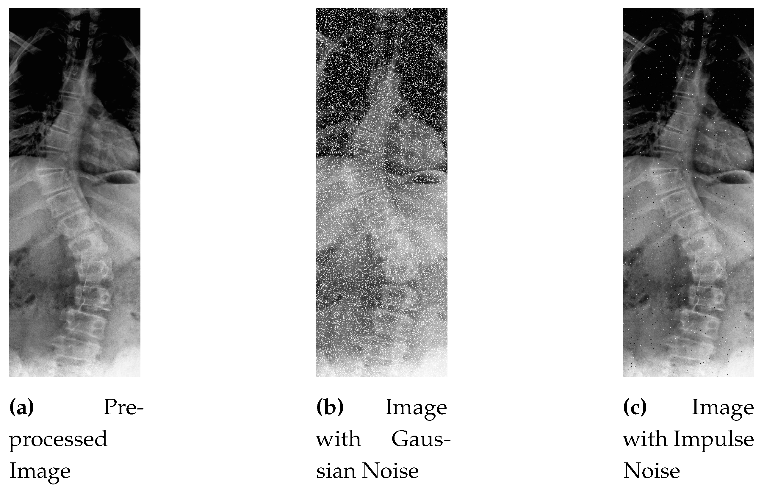
Figure 16.
Intelligently Cropped Image.
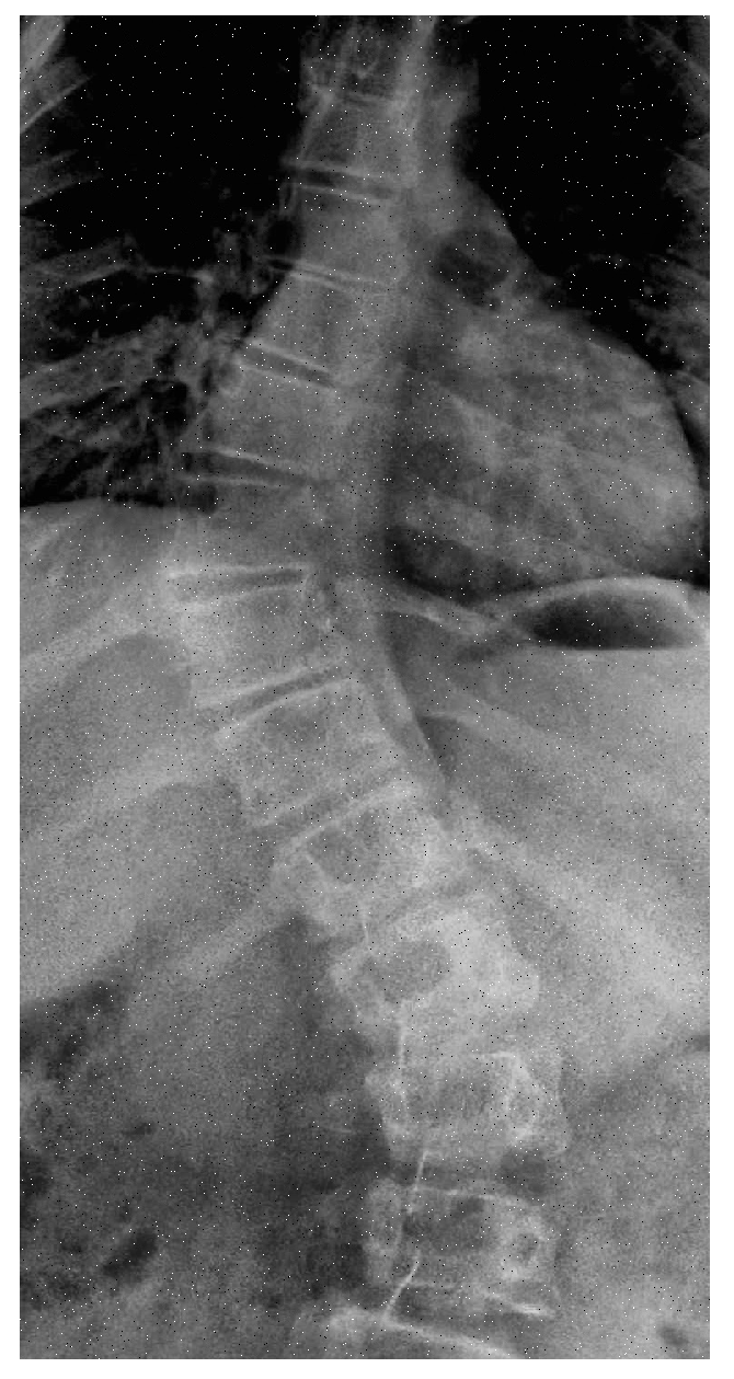
Figure 17.
Visualization of landmarks.
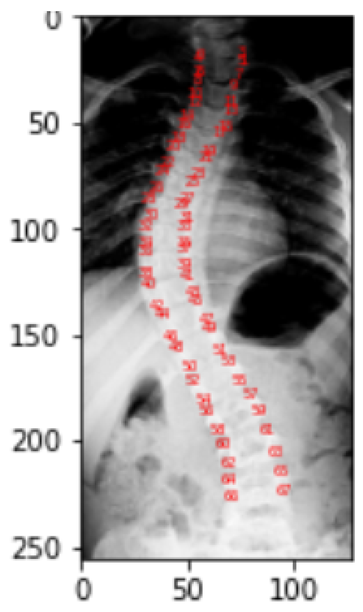
Figure 18.
Masking.
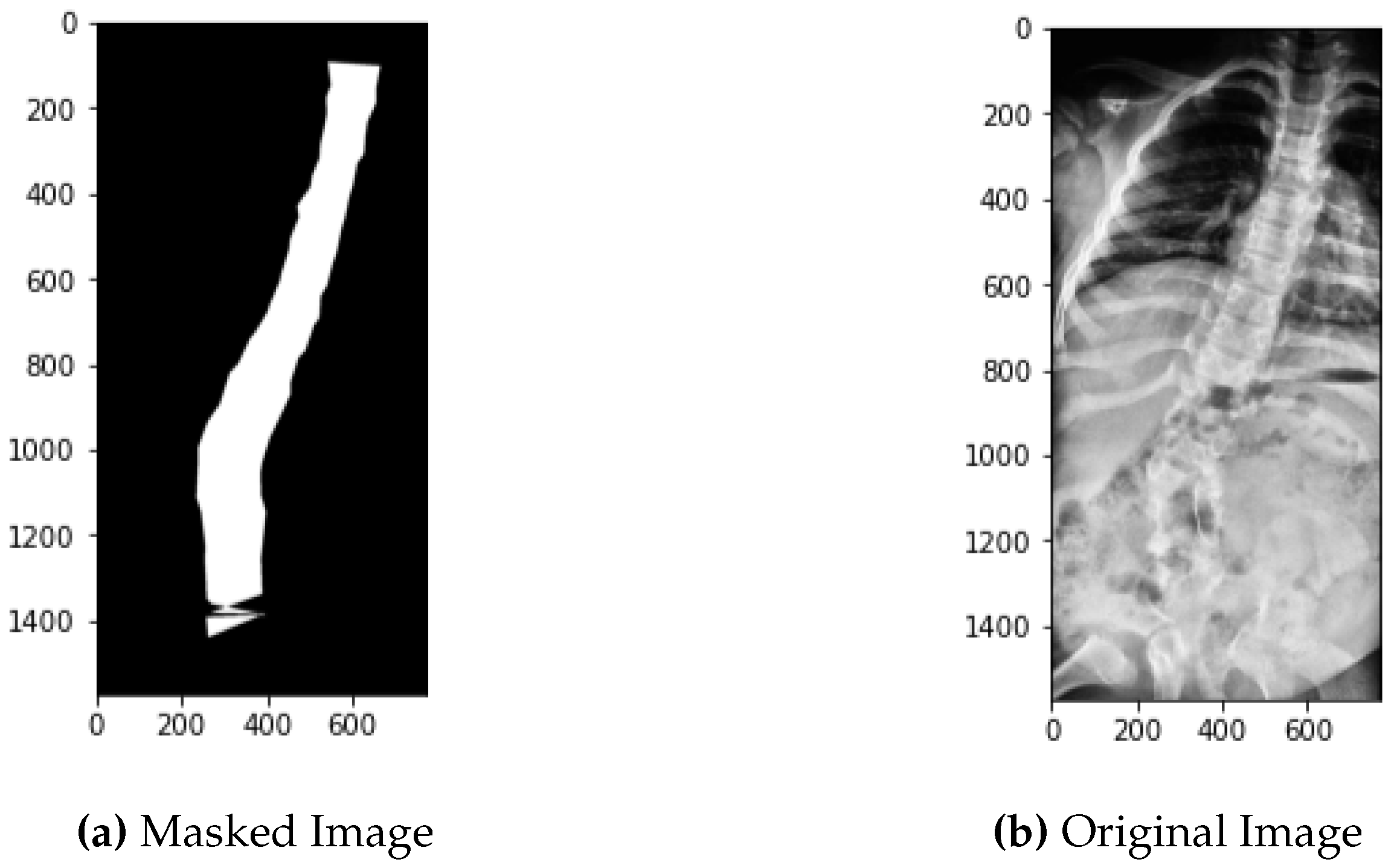
Figure 19.
Flipping vs Rotation.
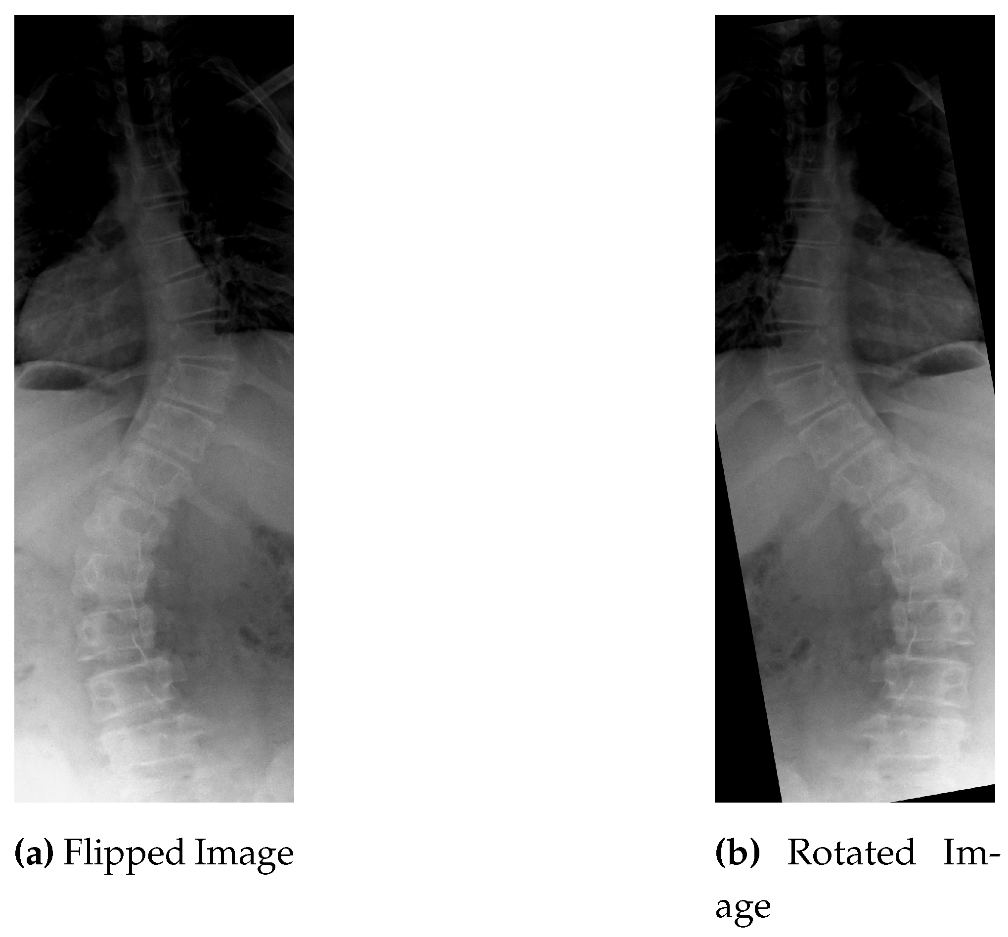
Figure 20.
Angle-1 Ground Truth vs Predicted Values.
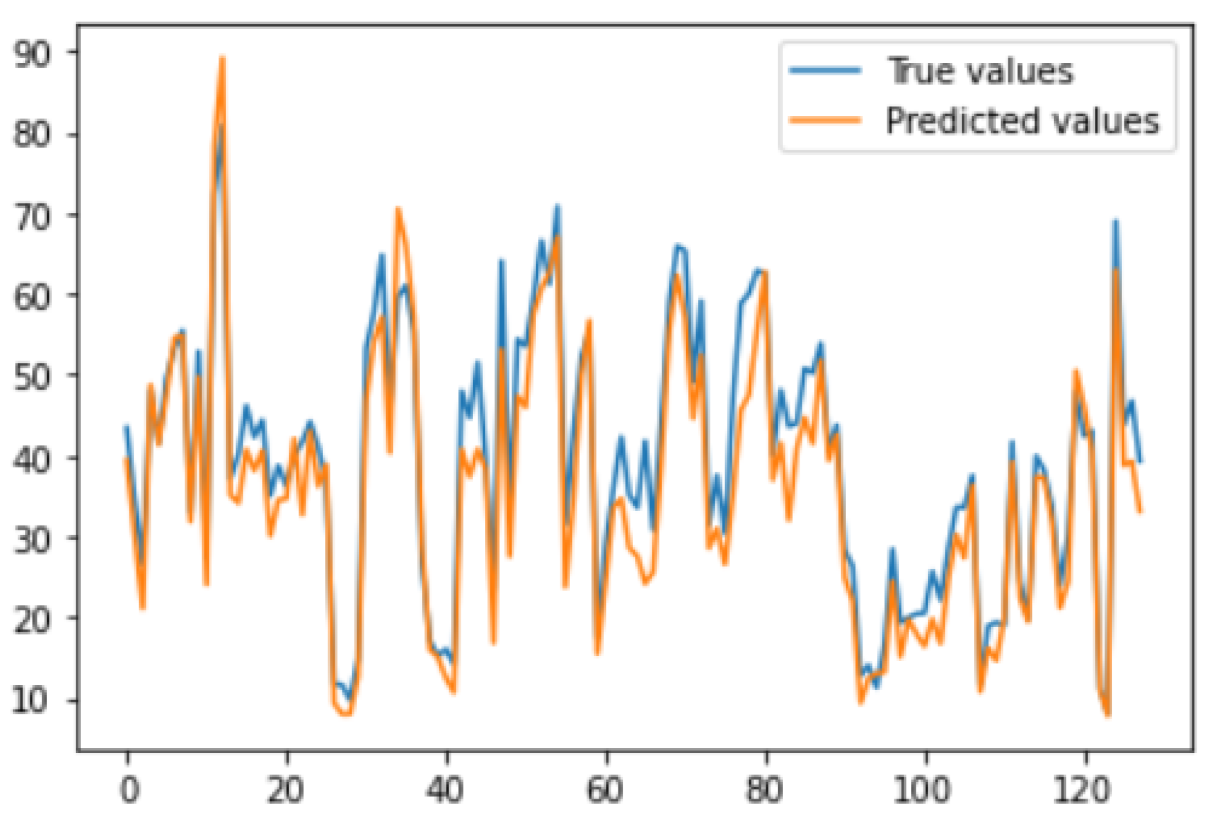
Figure 21.
Angle-2 Ground Truth vs Predicted Values.
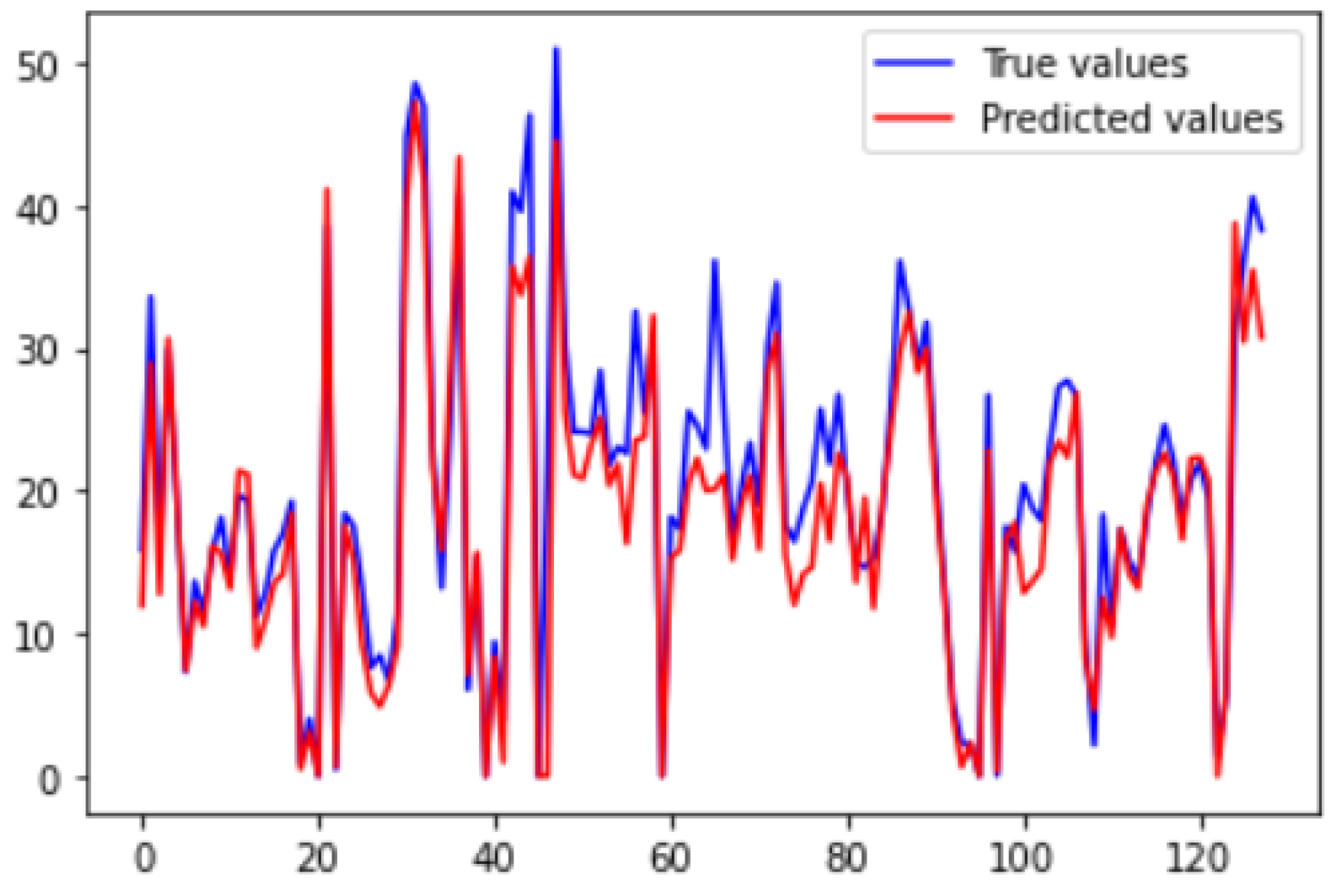
Figure 22.
Angle-3 Ground Truth vs Predicted Values.
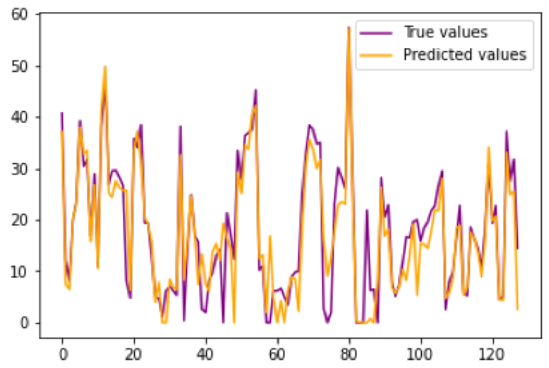
Figure 23.
Model Performance.
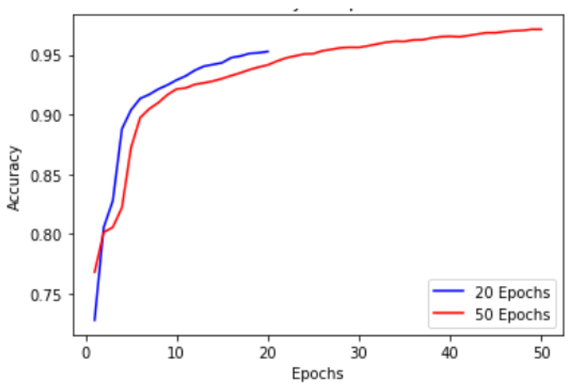
Figure 24.
Scatter Plot b/w Ground Truth and Predictions.
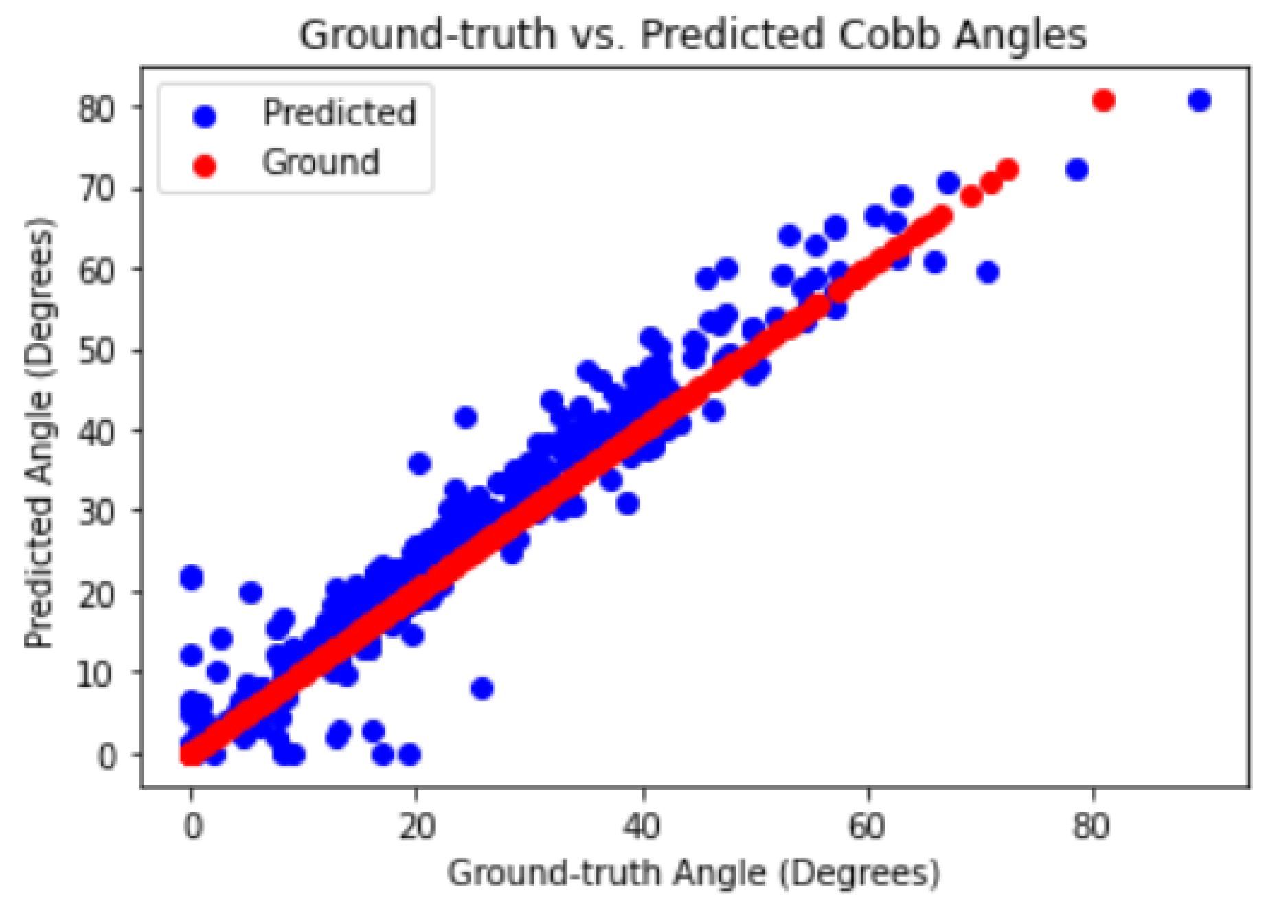
Figure 25.
Q-Q Plot b/w Ground Truth and Predictions.
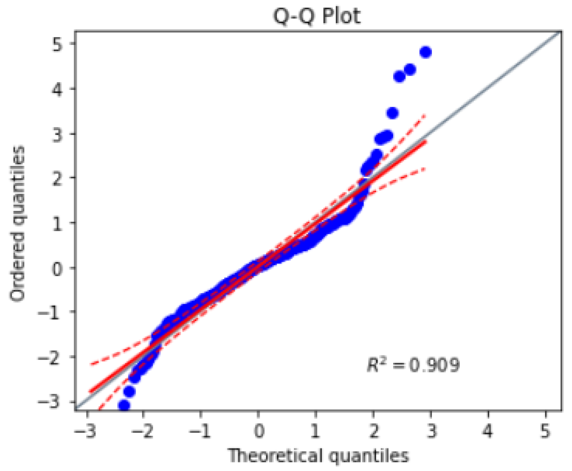

Table 1.
Comparison Table.
| Paper | Techniques | Dataset Type | Results | Limitations |
|---|---|---|---|---|
| [29] | CNNs Architecture based on Residual U-Net, Dense U-Net, Standard U-Net | X-ray Images | Residual Network gives segmentation Accuracy of . | Did not explored image reconstruction, enhancement and reorientation correction, noise in images |
| [33] | LCE-Net | X-ray Spinal Images | Segmentation as an task to give more information to estimate landmarks, approach is more reliable for both landmark and angle estimation | Require more information, increased computation cost |
| [34] | CNNs(4) with ResNet(152 layer) | X-ray Images | Accuracy With Adam Optimizer | Accuracy is achieved in Non clinical settings, can only detect single major curve, not minor curves, |
| [27] | CNNs with ReLU | X-ray Images | High degree of reliability when the Cobb’s angle did not exceed 90 degree | Intra-rate variability of model is 0, Identical output on identical input |
| [31] | U-Net based AI Method | X-ray Images | Validation Accuracy were recorded | Severity Classification stage is important and not included |
| [35] | CNNs comparison with Manual Measurement | X-ray Images, Manually labeled | Evaluation at the rate of 300 milliseconds | For Only Adolescent Idiopathic Scoliosis (AIS) not congenital, moderate bends, Lateral views |
| [32] | Bounding Box Object detector with FAST-RCNN | X-rays | Successful vertebrae detection before landmarks | Inter-dependency b/w vertebrae needs to find |
| [36] | U-Net and Convex Hull | X-rays | High real time performance | sensitive angle detection due to reduced image size |
| [37] | Support Vector Regression | X-rays | Direct angle calculation from image features | Supervised kernel learning required |
| [38] | Random Forest Regression | X-rays | Helping Clinician in angle succession of patients | Characterizing backbone in space |
| [30] | Cascade of two CNNs | X-rays | MAE of degrees | Manual Cropping Required |
| [39] | Btrfly-Net and U-Net Model | CT Scans | Overall accuracy | Progression of angle over time |
| [40] | U-Net ensembles | CT Scans | 9 out of 10 patients correctly graded | Higher computation cost, One image analysis take 8 mins |
| [31] | U-Net | CT-Scans | accuracy | Angle Progression Needs to work on |
| [41] | Variant of U-Net CNNs | Ultrasonographs | of measurements within clinical acceptance | Cannot detect angles greater than 45 |
| [8] | U-net | Radio-graphs | of verification dataset of spine | Angle calculation required to perform on whole spine |
Table 2.
Hyper-parameters used in the U-Net model.
| Hyper-parameter | Value | Description |
|---|---|---|
| Learning rate | Determines how quickly the model learns from the dataset | |
| Batch size | 64 | Number of images processed in each iteration of training |
| Number of filters | Determines the depth of the model and its complexity | |
| Dropout rate | Prevents over-fitting during training | |
| Kernel size | Determines the size of the convolutional filter | |
| Epochs | 50 | Determines the number of iterations |
| Validation Split | 15% | Split of training and validation set |
Table 3.
Unparalleled Comparison of Proposed Technique on a Shared Dataset
| Techniques | Dataset | Results | Constraints |
|---|---|---|---|
| CNNs[30] | 609-AP interior-posterior X-rays | MAE of 3.87 | Manual Cropping and larger running time |
| U-Net[31] | 609-AP interior-posterior CT-scans | accuracy | only detect angles |
| CNNs with 152-layers ResNet[34] | 609-AP interior-posterior X-rays | accuracy | Only detect major curves, not minor |
| Proposed Technique | 609-AP interior-posterior X-rays | accuracy with MAE of and computation cost of image is | Validations and clinical trials are required across diverse dataset |
Disclaimer/Publisher’s Note: The statements, opinions and data contained in all publications are solely those of the individual author(s) and contributor(s) and not of MDPI and/or the editor(s). MDPI and/or the editor(s) disclaim responsibility for any injury to people or property resulting from any ideas, methods, instructions or products referred to in the content. |
© 2024 by the authors. Licensee MDPI, Basel, Switzerland. This article is an open access article distributed under the terms and conditions of the Creative Commons Attribution (CC BY) license (http://creativecommons.org/licenses/by/4.0/).
Copyright: This open access article is published under a Creative Commons CC BY 4.0 license, which permit the free download, distribution, and reuse, provided that the author and preprint are cited in any reuse.


