Submitted:
08 August 2024
Posted:
13 August 2024
You are already at the latest version
Abstract
While in the past, especially numerical approaches such as regression models and p-values were utilized to investigate whether the functional form between age and happiness is linear or U-shaped in a given country, recent advances have shown that such approaches can be misleading, and graphical analyses should amend the analyses. However, these have the downside that they rely to some extent on subjective interpretations and are hardly quantifiable. If applied carelessly, they can be misleading as well. We suggest two easily computed statistics to combine graphical and numerical approaches. We demonstrate their usage with ESS data (N > 440,000) and show how they enable a more nuanced investigation of functional forms. Furthermore, we discuss how statistical uncertainty can be handled in the age-happiness debate and emphasize practical significance, which needs to be kept in mind.
Keywords:
happiness
; ageing
; functional form
; graphical analysis
; practical significance
1. Introduction
How does happiness vary by age, and does this functional form differ by country? These seemingly simple questions are the core of a decade-old research debate. Despite dozens of published studies, including hundreds of thousands of surveyed individuals and hundreds of countries, a consensus has yet to emerge. While some scholars claim that there is a U-shape in almost all countries (Beja 2018; Blanchflower et al. 2023; Blanchflower and Oswald 2009; Cheng et al. 2017; Graham and Ruiz Pozuelo 2017), others disagree (Bartram 2021, 2022; Becker and Trautmann 2022; Bittmann 2021; Kratz and Brüderl 2021). Interestingly, the data used to answer these questions is often common to multiple studies, yet statistical and methodological questions, such as the modeling strategy or the inclusions or omission of control variables, influence the results and interpretation. A recent publication has demonstrated that an over-reliance on regression coefficients and their respective p-values can distort the results and lead to questionable results, especially when graphical and descriptive methods support different interpretations (Bartram 2024). At this point, we would like to contribute to this methodological discussion regarding using graphical and descriptive approaches. They have the advantage of requiring fewer (statistical) assumptions and supporting a flexible interpretation, regardless of sample sizes or model specifications used (in contrast to regression-type approaches). However, graphical approaches are not generally accepted by everyone as they come with a more subjective part, leaving the interpretation up to each researcher, which differs from the classical and “hard” numerical statistics that appear to be precise and stringent. At this point, we suggest reconciling graphical and numerical approaches to some extent and outlining how they can amend each other. We suggest two common and easily computed statistics that help researchers decide flexibly whether the functional form between age and happiness is rather linear or not. These statistics have the advantage of being independent of sample size and not using (regression-computed) p-values. They are more nuanced and avoid a binary classification and thinking. We will discuss the problem of binary conclusions in empirical research in more detail and suggest alternatives. In addition, we would like to emphasize practical significance (in contrast to statistical significance), which is often forgotten in both graphical and numerical analyses (Mohajeri et al. 2020). We will demonstrate that some countries have a rather distinct functional form yet probably lack any practical relevance regarding the influence of age. This conclusion aligns with other studies that test the specific influence of various predictors on (un)happiness (Bittmann 2024). When age’s overall and total effect on happiness is tiny, the question about functional forms becomes rather academic as they have little real-life implications. We suggest discussing these aspects openly so that research is not disconnected from reality. This is not a proposal to shut down the debate of functional forms but rather the contrary. It appears to be highly relevant to understand in which countries age has lost its influence on happiness, why this has happened, and which mechanisms are relevant.
Summarized, the following paper has three research questions: First, how can we assess the functional form between age and happiness graphically and numerically? Second, what is the overall influence of age on happiness (practical significance of age)? Third and final, how are functional forms and the overall influence of age on happiness related to each other? Using a large-scale European dataset (N > 440,000), we will answer these questions empirically and make suggestions for advancing the age-happiness debate in general.
2. Theoretical Aspects
This section has two main purposes. First, we give an overview of recent developments in the age-happiness debate to see what has been research and how in the past. This is relevant to see where research gaps and potential problems lie and how they can be amended. Second, we discuss in more detail the implications of our research approach and how binary conclusion traps can be avoided and we suggest a way to handle uncertainty in this research debate.
2.1. Recent Developments and Research Agenda
Thanks to the ongoing research on the influence of age on happiness, there have been major developments. Here, we will briefly summarize the main advances in the past few years.
- Control variables’ function has been explained in much more detail (Bartram 2021; Kratz and Brüderl 2021). While in the past, the addition of control variables such as gender, education level, health, or marital status was rather common in regression models to the main predictors (age or higher-order terms such as age-squared), convincing arguments have been put forward to remove most such controls from the models. As has been shown, no classical controls are required to estimate the total and causal effect of age on happiness as there are no antecedents of age. Adding more variables to the model can be relevant to estimating meditation pathways and explain how and why age influences happiness; however, if the general functional form is to be estimated, these should be removed to avoid overcontrol bias (Elwert and Winship 2014). However, some variables can still be helpful to account for period and survey effects.
- It is much clearer now how careless interpretation of regression models can be misleading when estimating functional forms. Especially only relying on the statistical significance of some coefficients is not a valid way to prove such forms. To start with, explorative attempts that do not rely on statistical significance at all but on cluster approaches have shown that functional forms can be diverse and that at least three major functional forms are present, disproving older claims that the U-shape is general and valid everywhere (Bittmann 2021). Follow-up studies have also shown that the approach to explain functional forms solely based on model coefficients can be misleading as even for highly linear forms, squared terms of age can still be statistically significant (Bartram 2024). The role of sample sizes has also been considered to avoid wrong conclusions. This connects to the debate about the problematic usage of p-values in statistics and that more nuanced approaches are highly encouraged (Wasserstein et al. 2019). More details are outlined below in section 2.2.
- Based on these developments, arguments have been made to avoid emphasizing the classical regression-testing context where only coefficients are evaluated numerically. Instead, graphical interpretations are flexible and accessible as a highly relevant addition to numerical approaches. They can demonstrate directly, for example, that higher-order terms’ statistical significance does not guarantee a non-linear functional form. Furthermore, they encourage a more nuanced discussion and they avoid binary classifications.
While these developments are welcome and advancing the field, we would like to make a few additions and reconcile numerical and graphical approaches to some extent. While beneficial, we would like to demonstrate how graphical methods can also be misleading if applied carelessly and to show how numerical analyses are still beneficial. Furthermore, we would like to emphasize practical significance (compared to statistical significance). Even coefficients with very small p-values can be meaningless in the real world, which should be part of the general discourse. We should make it more salient why and how much the age-happiness relationship matters (and how this differs between countries).
2.2. Moving to a World Beyond Binary Conclusions
In the past few years, a shift has happened in statistics. More and more researchers agree that binary conclusions, which are mostly facilitated by an unhealthy focus on p-values and other “hard” statistics that support such conclusions (“the p-value is smaller than 0.05; hence I conclude that my findings are true…”) are problematic and do more harm than good. This shift in thinking about uncertainty and statistics regards the type of statistics we should compute, report, and interpret, such as p-values, confidence intervals, or measures of effect size, and how uncertainty in general should be addressed. Unfortunately, this thinking has not yet quite reached the age-happiness debate. Too many previous studies easily reach binary conclusions, such as that the statistical significance of a squared regression term leads to the conclusion that a functional form must be (reversed) u-shaped (Bartram 2024) or that countries can be easily grouped in clusters (Bittmann 2021), resulting in either-or classifications with no room for in-between. We argue that such binary thinking is harmful when discussing complex and messy aspects such as functional forms, as, in reality, these forms are never truly “linear” or anything else. For example, linearity is a mathematically defined term that data from real data can never reach, only approach to a certain degree. When in doubt, researchers should report this transparently and discuss the degree of similarity, potential biases, and especially the uncertainty around their estimates. Only this facilitates an open and honest discussion about phenomena in the real world that we, as researchers, would like to describe and assess statistically. Introducing graphical ways of interpretation to the debate is a step in the right direction as “a picture is worth a thousand words”, which enables nuanced and more complex conclusions than a few numbers ever can. However, as explained before, such an approach is also limited. We want to amend these graphical approaches with some statistics yet not fall into binary decision traps again. However, this endeavor also comes with costs. When discussing statistics in the following, there are no clear-cut guidelines for when an effect or change is “small” or “large”. Researchers are so used to strict guidelines (“a p-value below 0.05 shows a real effect” / “an effect size around 0.50 is of medium size”, etc…) that it seems out of place to make such a statement that reported numbers cannot be easily evaluated or classified. For the current analyses and probably large parts of the overall debate, we recommend avoiding absolute classifications but comparing numbers and effect sizes to each other. For example, when multiple countries are compared within one study, one can see that some countries have a more linear shape than others. When talking about the total effect of age on happiness, one can potentially conclude that age matters more in some countries than others. These relative comparisons avoid binary conclusions and are more nuanced as they fall onto a continuous spectrum, which enables fine-grained conclusions. When a study only includes a single country, one can reference previous research results and see whether effect sizes are smaller or large but not “small” or “large”. Leading a discussion in such a way provides relevant information to readers yet is nuanced and takes the complexity of the real world into account. While it may take a while for experienced researchers to get used to talking about data and statistics in such a way, we argue that uncertainty and relative comparisons should be embraced to avoid past mistakes and move on as a research community.
3. Data, Variables, and Methods
3.1. Data, Sample, and Variables
In the following, we use ESS data from the last ten rounds (ESS 1, edition 6.7, to ESS 10, edition 3.1). The ESS provides high-quality data for more than thirty European countries. While adding even more countries from other continents and regions was possible with further datasets to outline our points, the ESS is adequate. Especially since graphical interpretations are relevant, showing even more countries might be overwhelming. Furthermore, as older studies have shown, there are diverse functional forms for age and happiness in Europe. Due to the long-running nature of the ESS, many countries are included multiple times in the dataset, which provides further insight and statistical power. To be concrete, only countries that have at least two non-consecutive participations are included. Furthermore, only individuals aged from 18 to 80 are included. This ensures that there is also enough evidence in the oldest cohorts, as a very low number of very old participants could distort functional forms due to outliers. The resulting sample for all analyses hence includes 33 countries with a total of 440,160 participants. To avoid the influence of period effects and account for differences in survey methodology, the ESS round will be included as the sole control variable in the following analyses.
The dependent variable is happiness (“How happy are you?”), which is measured on an 11-point Likert scale with values from 0 (“extremely unhappy”) to 10 (“Extremely happy”). This measurement is harmonized over all waves and countries and provides a well-established measurement of happiness or life satisfaction. The main independent variable is age in years. Individuals with missing values are removed from the analyses (listwise deletion). However, the share of missingness for both variables is extremely low (less than 1% each).
3.2. Strategy of Analysis
3.2.1. Graphical Approach: Local Polynomial Smoothing
The goal of this analysis is to show how graphical approaches can be both beneficial and misleading. Furthermore, it attempts to demonstrate how graphical and numerical approaches can complement each other. To be most flexible, one could start with a simple scatterplot between happiness and age, as this is purely descriptive and does not make any assumptions. However, given that both variables only contain a limited range (especially happiness with only 11 possible values) and a very large number of individuals in each country (N varies between 3,706 and 31,996), every potential point in the graph would be occupied, making a graphical interpretation close to futile. To resolve this issue, local polynomial smoothing is a potential solution (Cleveland and Loader 1996; Fan 1992). For as many points as specified by the researcher (typically 25 to 100) over the range of the x-variable (age, in our case), a regression model is estimated at each point, and a kernel function weighs the influence of each observation. The intercept of the computed regression is then used as the result at this x-value. By repeating this step for all specified points, the immense information of the scatterplot is reduced to a rather small number of points, which can be used to fit a line, arriving at a simple line graph that is easy to interpret as the data is condensed into this fitted line, showing the functional form between x and y variable. A similar approach is LOESS or LOWESS, which could also have been used. While this approach is sensible and useful, it can still be misleading. Foremost, as with any graph, scaling matters. Should a graph always start with zero or not? When different countries are compared to each other, is it sensible to put them all on the same scaling or is it better to use flexible scales as to underscore smaller differences between countries? Below, we demonstrate how different answers to these questions can influence how graphs are read and interpreted and some advice is given. Furthermore, when using polynomial smoothing, there are several parameters that the researcher has to set (which is sometimes done automatically by the software). For example, the number of points to estimate the local function has to be specified, as well as the type of kernel algorithm or the degree of the regressions used in the computations. However, these specifications are usually rather technical and have no large influence (as long as no extreme values are chosen). In any case, we recommend to be transparent and discuss such decisions when discussing results so readers have the change to think about this and contemplate alternatives, which might lead to different conclusions.
3.2.2. Numerical Approach: Absolute and Changing R²
For the numerical approach, we would like to focus on three distinct aspects: first, what is the functional form between age and happiness, for which we use the relative change of R². Second, we would like to see the total and absolute relevance of age to explain happiness, for which we use the R² value of a well-fitting regression model. Third and final, we would like to discuss how these two statistics relate to each other and what this can tell us about different countries and contexts. Since we work with numerical values, it is also crucial to talk about some kind of “effect” size when comparing numbers, which is also taken up at the end of this section.
We start with the functional form (relative change of R²). We would like to have a numerical approach that does not rely on p-values or solely on the coefficients in a regression model and avoid coarse or binary classifications. We compare the empirical functional-form with a range of theoretical ones and select the one with the best fit. This goes back to the problem of statistical fit in a regression model, for which a wide range of statistics has been developed. As our models have only one main predictor (age, or derived higher-order terms), we would like to keep things simple and work with R² (while other fit measures might work similarly). R², or the coefficient of determination, is easily computed in an OLS regression model as one minus the residual sum of the squares divided by the total sum of squares (Gujarati and Porter 2010). When the model has exactly one predictor, this can also be shown graphically on paper. R² is bound between 0 and 1 and adding additional predictors to the regression models can only increase its value but never decrease it. Therefore, adding “useless” predictors with little predictive power can never make the model fit worse, as R² does not consider model parsimony. For our means, this is completely fine. Since we are mostly interested in the distinction “linear-shape” vs “non-linear shape”, we compare the linear model to a more flexible one. In our case, we decided to use the cubic model1 as it can model either a u-shaped form or even more complex forms. By comparing the model fits between the two models, we can assess, numerically, whether a non-linear functional form is more plausible than the linear one. It works as follows: Imagine the most simple case, a highly linear relationship with exactly one independent variable. This predictor perfectly explains the functional form (except for random errors, which will always be present in real-life datasets). Adding higher order terms to this model (the squared or cubed term of the predictor) will not change R² in any significant form. However, keep in mind that “significant” does not mean “statistically significant” but needs to be discussed and assessed by the researchers! We call this the relative change of R² (which can be expressed as a percentage change from the base). Hence, adding a higher-order term will hardly increase R² if the relationship is truly linear. This is rather different if the relationship is (inversely) U-shaped or even more complicated. While the linear model specification will usually have some explanatory power, adding one or more higher-order terms will greatly improve the model fit (again, in the view of the researchers). Hence, the relative percentage change of R² will be larger. We argue that this relative change of R² is a simple way to estimate whether the functional form is linear or not. If the change is rather smallish, the fit is linear; if the change is larger, it is not. This is the main claim we are testing empirically further below. We will demonstrate practically how assessing “smaller” or “larger” works in a multi-country comparison when absolute judgments are to be avoided. Since these percentage changes can be huge, especially when base levels are very small, logarithmising them can be beneficial to avoid large numbers.
For the approach as just explained, there is a caveat, which is the second main argument of this paper, which is about practical significance. The idea is to study both the relative changes in R² and the absolute R² (from the best-fitting model available). This means, regardless of how complex and well-fitted the regression model is (potentially adding squared, cubed, and even further terms), if the final R² value is low, there is an overall very limited influence of age on happiness. This is relevant for practical questions. Even if the functional form between happiness and age was perfectly U-shaped, if the total explained variance of happiness by age is very low, why should one care much about his fact? The happiness an individual reports is, to a very small extent, dependent on age, and other influences might be much more relevant. This connects the age-happiness debate to a broader question: If we are interested in studying happiness and which factors explain and predict it, age might be negligible (at least in some countries). This fact must always be kept in mind; otherwise, this entire debate and literature can degenerate into an overly academic discussion detached from real life. That is why we are also interested in the total R² that a well-fitting model has. As explained above, since R² can never get lower, even if higher-order terms are added to a perfectly linear model, we decided to use the R² value of the cubic model as a measurement of absolute fit and relevance of happiness. We would like to emphasize that this second numerical value is also rather meaningless without context. We suggest to either compare these values to each other in multi-country comparisons or compare them to the influence of other predictors of happiness (for example, gender, health, or marriage status). By doing so, more nuanced insights are possible, as other studies have attempted to test a large set of predictors to explain happiness (Bittmann 2024; Doherty and Kelly 2010; Haller and Hadler 2006).
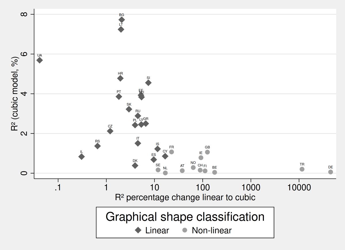
Lastly, we would like to test how relative changes in R² (functional forms) and absolute values of R² (total influence of age on happiness) are related. One previous publication indicated graphically that there might be a relation as more developed countries, also with a higher HDI, usually display non-linear functional forms, while countries with lower HDI have more linear forms (Bartram 2024). Another publication that attempted to sort functional forms into clusters also demonstrated this numerically (Bittmann, 2021). This gives a first hint that there might be a deeper relation to why some countries have linear shapes while others have not. As in more developed countries, the practical significance of age for happiness us lower due to social welfare systems, such as health-insurance or pension schemes, we would also expect a relation between total explained R² by happiness and the relative explanatory power. This research question is tested numerically and graphically. Numerically, the correlation coefficient is computed for absolute explained variance in the cubic model and the relative improvement of R² from the linear to cubic model. Graphically, this is done by plotting these two values against each other in a scatterplot, separately for each country. If there is a relationship found, this could hint for structural, social, or cultural differences between countries that deserve attention. Furthermore, one can see which countries are similar to each other and which are rather different in this relationship. Finally, this graphical form of presentation, again, underlines how graphical approaches can be beneficial for nuanced interpretations, especially when multiple countries or data points are to be compared.
All analyses are conducted using Stata 16.1, and do-files are available upon request.
4. Results
4.1. Graphical Approach: Local Polynomial Smoothing
As described before, the first part of the analysis is a graphical interpretation. For comparison, the functional form between happiness and age has been computed for all countries in the ESS data using local polynomial smoothing. These results are shown in the appendix (Figure A1 and Figure A2). Since this has been done before in other publications, it is only depicted as a reference so one can later compare the numerical results for all countries to the graphs. What is of greatest interest to us is to see how graphs can still be misleading if applied carelessly. This problem is not the method itself but rather the scaling of the axes (Bryan 1995). To demonstrate this, two countries, Portugal and Germany, have been selected from the dataset. On paper, these countries are comparable. They have participated in every ESS round since the start, and many observations are available (31,224 for Germany and 16,350 for Portugal). Both have been members of the European Union for more than 35 years and have a high Human Development Index (0.942 / 0.866 in 2021). However, when the functional form of happiness and age is investigated, the graphical approach yields two different conclusions. We start with Figure 1, the upper panel (Flexible y-scales). This scaling approach uses different y-scales for both countries. The benefit is that within-country differences are emphasized and details are revealed, however, a cross-country comparison becomes difficult, potentially misleading.
For Portugal, we observe a highly linear and monotonic decline in happiness over the age course. The older people become, the less happiness they report. Based on this graph, one would hardly ever assume that a U-shaped relationship is present in Portugal. However, for Germany, the conclusions are different. In their youth, individuals are rather happy, but the older they become, the less happy they are. There is minimum value for individuals aged around 50 years. Afterward, there is a turn, and happiness rises to the age of about 70. Then, happiness starts to decline again. This is an ideal case of the classical U-shape, especially in the middle part of life. However, it should be outlined how this interpretation can change as soon as we change the scaling of the y-axis, measuring happiness. As shown in the upper panel, the axes are different between both countries. In Portugal, it ranges from 7.5 to 6.0 but in Germany only from 7.4 to 7.1. If we look at the global maximum and minimum of the distribution in the graphs (compare also Table A1 in the appendix), we see that these values are 7.48 and 6.33 for Portugal (range 1.15) but 7.38 and 7.20 for Germany (range 0.18). When we force the same scaling in the lower panel of Figure 1, our conclusions are rather different. Portugal displays the wider range of happiness and remains unchanged. However, if the same scaling is forced on Germany, the distinct U-shape has mostly vanished. If looking only at this new graph, it becomes rather difficult to see the U-shape as it is rather flat. What are the implications of this? While it has been well-known that one can create misleading graphs when changing scales in graphs, there is no clear-cut recommendation. In this example, both scalings have benefits and disadvantages. We suggest: when comparing different countries to each other, using the same scaling appears helpful to enable a fair comparison on the same scale. If only a single country is of interest, a flexible scaling can help reveal nuances and details. In any case, researchers should think carefully about this issue and handling it transparently, outlining why they have chosen a certain scaling and how the interpretation or conclusions changes when the scaling is changed.
The problem of scaling also relates to the next sections where numerical approaches are discussed. When considering the identical scaling, one could conclude that the overall range the aggregated happiness falls into is much larger in Portugal than in Germany. In other words, the variation over the average life-course is much larger. This can also be quantified numerically, as we have already done above. In the appendix (Table A1), we report the range of aggregated happiness for all countries in the ESS. To assess whether these within-country variations are rather large or not, there are some hints in the literature. Jebb et al. (2020) argue: “For our Cantril ladder scale, respondents reported (and probably thought) in terms of the nearest whole scale point from 1 to 10. Therefore, it seemed that differences below 1.00 should be considered quite small.” (p. 296). Given this reference, the variation is small in Germany but not so in Portugal. However, to relate to what we have written in section 2.2, we suggest avoiding absolute comparisons or judgments but keep a relative one. What can be said without a doubt is that the variation is much larger in Portugal than in Germany. As discussed in more detail below, this suggests that age matters more in this country to explain happiness than in the other.
4.2. Numerical Analyses: Absolute and Changing R²
As outlined in section 3.2, we have proposed some relevant statistics to judge numerically how relevant the influence of age is on happiness. We show our results for all countries in the ESS in Figure 2 for a convenient overview. Two main statistics are presented and discussed; for a complete overview, refer to Table A1 in the appendix.
First, we would like to talk about practical significance and the overall influence of age on happiness. Note that this is not about the functional form between happiness and age but only on the relevance of age for happiness in a given country. To achieve this we concentrate on the absolute R² explained by the cubic model.2 The larger this number, the better age can explain the variation in happiness that is due to the influence of age. Note that the ESS round is included as a control variable. However, this specific influence has been subtracted from the result, so the reported R² values are the pure influence of age and its derived terms (net influences).3 Results are presented in Figure 2 (lower panel). What we see is that the highest values are found in Bulgaria, Lithuania, and Ukraine. In these countries, more than 5% of the total variation in happiness is explained by age. This is very different in other countries, such as the Netherlands, Germany, or Finland, there not even 1% of this variation is explained by age. This also relates to what has been discussed before in the graphical approach, that is the overall variation within a country. The conclusion is clear, age matters more for happiness in some countries than in others. In the ESS setting, not the absolute values of R² can be interpreted but more so the relative comparison between countries. For example, as the value is 1.1 in the United Kingdom but about 7.7 in Bulgaria, one can conclude that age matters about seven times more for happiness in Bulgaria than in the UK, which outlines a huge difference between these two countries.
The next question we would like to answer is the functional form between happiness and age. Here we utilize the change of R² as soon as the assumption of a linear functional form is abandoned (by adding the squared and cubed term of age to the model). This is done as follows: R² is computed for the linear and cubic model, and both R² values are stored separately for each country (again, ESS round is included as the sole control variable to account for period-effects or other unwanted influences, such as changes to survey quality or methodology over time). The percentage change from the linear to the cubic model is computed, and the logarithm is taken. This is necessary since, for a few countries, the percentage change is huge as the first value is very small and close to zero (hence, a minuscule change can still result in a large percentage change, which could distort the results). This statistic is relevant to check whether a functional form is linear or not, regardless of the absolute influence of age on happiness. Note that absolute changes below 1 percent become negative numbers due to the logarithm taken. Based on this statistic (Figure 2, upper panel), the countries that have the least pronounced linear shapes are Germany, Turkey, and Belgium. The most linear ones are Hungary, Ukraine, and Lithuania. When comparing this information in Figure 2 to the functional forms in the appendix, we can see a good congruence between graphical and numerical results when only the functional form is of interest, regardless of the total influence. Note that this always is a relative comparison, meaning that the functional forms are less-linear in some countries than in others. We do not believe that an absolute classification is target-oriented. We would argue that this is a clear benefit of the approach we have just introduced. Instead of relying on p-values, which often lead researchers to binary conclusions, our approach is more nuanced and provides a continuum for fine-grained comparisons with an inherent meaning. This can be used for between-country comparisons (such as in our case) but also for within-country comparisons (for example, when data from multiple points in time in available for a single country. A final benefit of our approach is that control variables can be included like in any other regression model, which means that the statistical analysis part is easy to handle and well-known to most researchers.
Next, we would like to relate these three statistics to each other: log. R² changes from the linear to the cubic model (1), absolute R² values of the cubic model (2) and the range of happiness of aggregated data (3, this last statistic is reported in Table A1 in the appendix). To do this, Pearson’s r is computed to measure the correlation between these three variables; results are reported in Table 1.
Figure 2 already indicates that countries with a high percentage change show a low total explanatory power of age, and indeed, there is a moderate negative correlation (Pearson’s r = -.559). Regarding the range of happiness and the absolute R² value, we observe a rather strong correlation (.94). We can conclude from this that in countries with a large variation of happiness over aggregated life-courses, age in general explains more happiness than in countries with low variation. What we can do in a final step is plot these statistics against each other for each country using a scatterplot. But first, we have also attempted to classify each country into linear and non-linear shapes based on Figure A1 and A2. Apparently, this is a subjective classification that is not written in stone. And again, binary classifications as this one can hide various nuances and are, in general, not encouraged, as they undo the benefits of the graphical approach. However, for this demonstration we would like to use this approach as it is quite relevant for the following scatterplot (Figure 3). Countries classified as having a linear relationship are BG, CY, CZ, DK, EE, ES, GR, HR, HU, IL, IS, IT, LT, LV, PL, PT, RS, RU, SI, SK, UA. All others are classified as either having a non-linear, U-shaped, or even more complex functional form. By doing so we can exploratively check whether any special patterns are present, which might benefit conclusions or further research studies.
First, note that the x-axis is logarithmic due to the wide range of numbers presented here. In contrast to Figure 2 (top panel), we have decided to plot the original values with a log-scale instead of logarithmising the values first for the sake of a clearer presentation. We see that countries classified with a linear shape have average values between 1 and 10% improvement in R² from the linear to the cubic model. For the non-linear countries, these improvements are usually between 10 and 100%, with two outliers with extremely large values. While this might seem impressive first, it is rather trivial as the base of the change is tiny and very close to zero. All countries classified as non-linear have absolute R² values between very close to zero up to about 1.8%. They all lie closely together at the bottom of the figure. However, this is rather different for the other countries as they have a wider range, up to almost 8% of total explanatory power. Regardless of the graphical classification, we believe that Figure 3 has much benefits as it enables are more nuanced interpretation. As we see, there is a wide range of values and most countries fall between 1 and 100% improvement by switching from the linear to the cubic regression model. This highlights neatly that the question of linearity in the functional form between age and happiness is not so much binary as rather a continuity. While a purely graphical interpretation as in Figure A1 and A2 is beneficial, Figure 3 summarizes the information for many countries. Especially when comparing countries, researchers should be aware of such graphical forms of interpretation and consider them as alternatives or amendments to numerical approaches.
5. Discussion
The main purpose of the current study is to reconcile graphical and numerical approaches when studying the functional form between happiness and age. In the first part, we demonstrated that graphical approaches, such as local polynomial smoothing, are highly beneficial to visualize functional forms flexibly. We suggest this is always the first step in an analysis since graphs can quickly summarize a large dataset. However, we have also demonstrated that reaching a conclusion through a graph can sometimes be challenging, especially when different populations are to be compared. Furthermore, they have the downside of producing a large number of graphs and comparing many countries can be difficult. As explained above, we suggest researchers to stay transparent and explain and justify various decisions, such as the choice of the axes scaling.
Consequently, we have dedicated the second part of the paper to suggesting some statistics that help characterize functional forms. These measures are quickly computed in any modern statistical software package, well-defined, and easily understood by a broad range of researchers. They do not depend on sample size or p-values, which still too often encourage binary conclusions. Using the statistics together, one can characterize whether a functional form is rather linear or not and whether the independent variable influences the outcome in a way that has any practical significance. We want to underscore that this last point has been neglected by research in the age-happiness debate. Our results indicate that the total amount of variation in happiness explained by age is extremely low and, for many countries, even below 1%. Therefore, the functional form between age and happiness is without any practical significance. In these countries, the variation of happiness due to a different age is so low that no intervention can make any practical difference, and the question of functional forms becomes rather academic. This finding is in line with another study that tests the influence of age on happiness in Germany, using high-quality panel data. Even in a bivariate model without further controls, age explains only about 0.58% of the overall variability in long-lasting unhappiness (Bittmann 2024). Based on these findings, it is relevant to refer back to other studies that do include control variables, such as education, marital status, health, or even social origin. Apparently, these more complex models will also explain more variance in happiness as they include other factors, some related to age, others not. They are able to explain, to some extent, how and why age can influence happiness. Yet, these are different questions. If we are interested in the pure and overall effect of age, we have demonstrated that this influence is tiny in some countries.
Of course, this does not mean that the study of age and happiness is meaningless, but the aims are different. For example, age’s influence on happiness in total, measured with R², is about 580 times larger in Bulgaria than in the Netherlands, hinting at rather different processes and mechanisms that must be active. It would be highly relevant to explain why age matters more in some countries than others and to test whether this changes over decades. As the results indicate, the influence of age on happiness decreases with a country’s prosperity and human development. As no mechanisms have been tested in this study, researchers are free to come to their conclusions about which factors might matter and why this is the case. Although the age-happiness debate continues, there is no end of relevant research questions.
Finally, the limitations of the study are summarized. Given the constraints of scope and data, we have limited ourselves to a discussion of whether a functional form is more linear or not. More complex forms may be possible. Nevertheless, as these are often difficult to characterize, even from a purely descriptive standpoint, we have omitted these questions. Especially since the age-happiness debate is mostly about linear and U-shaped forms, this is adequate, even though more research about more complex forms might be beneficial in the future. So far, only European countries are included in the present analyses. An extension to other regions might be interesting to gain more insight. However, as there are already rather diverse functional forms in Europe, this should be a manageable limitation of the study.
6. Conclusion
This paper outlines how the functional form between age and happiness can be investigated using graphical and numerical approaches. We have demonstrated that other measurements than the classical regression coefficients can be used to characterize functional forms and differentiate between linear and no-linear (U-shaped) forms. These two measurements are: first, the change in R² from linear to cubic models (or derived version, such as the percentage change or the logarithmized version thereof). This measurement is useful to distinguish linear and non-linear forms. Second, there is the absolute R² explained by a model with adequate complexity (by adding higher-order terms). This measurement is useful to indicate whether age influences happiness and how large this total influence is. Taken together, we propose that combined graphical and numerical analyses have multiple advantages compared to a pure regression approach, which also avoids certain downsides, such as an overreliance on statistical significance and potentially misleading comparison of regression coefficients. By at least adding suggested measurements, a more nuanced discussion becomes viable. We hope these propositions advance the ongoing age-happiness debate and put neglected aspects, such as the issue of practical significance, into focus. We hope that future research embraces uncertainty more and attempts to avoid binary or crude classifications. Current methods, both graphically and numerically, provide ways to come to more detailed interpretations, which can lead to new insights and advance the overall debate.
Declarations
The author did not receive support from any organization for the submitted work. The author has no relevant financial or non-financial interests to disclose.
Acknowledgments
David Bartram read an early version of the draft and also gave helpful comments.
Appendix A
Figure A1.
Functional forms by country (part 1). Source: ESS1-10. Post-stratification weights applied. 95% confidence intervals included. The x-axes measure age in years, the y-axes happiness.
Figure A1.
Functional forms by country (part 1). Source: ESS1-10. Post-stratification weights applied. 95% confidence intervals included. The x-axes measure age in years, the y-axes happiness.
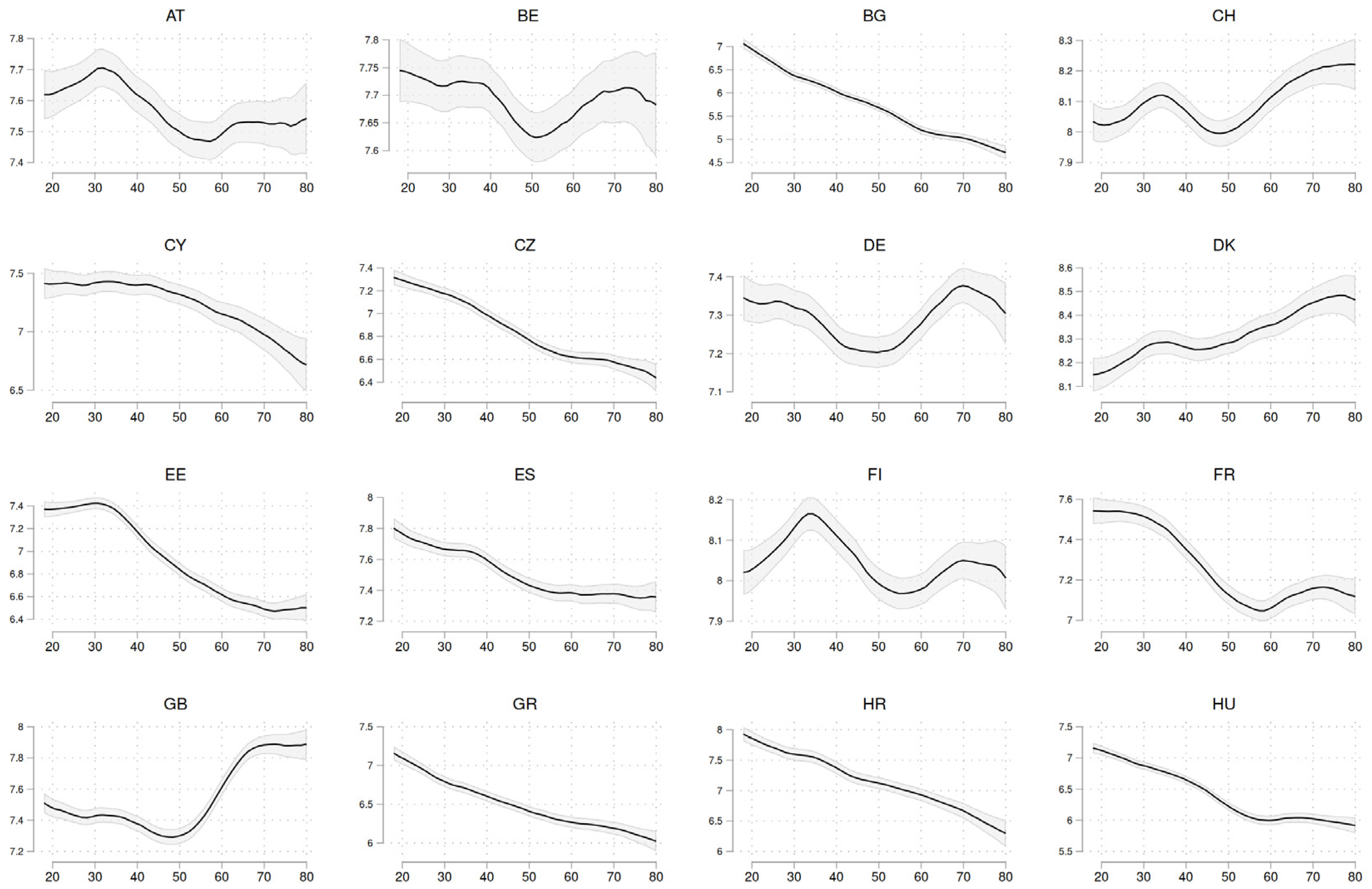
Figure A2.
Functional forms by country (part 2). Source: ESS1-10. Post-stratification weights applied. 95% confidence intervals included. The x-axes measure age in years, the y-axes happiness.
Figure A2.
Functional forms by country (part 2). Source: ESS1-10. Post-stratification weights applied. 95% confidence intervals included. The x-axes measure age in years, the y-axes happiness.
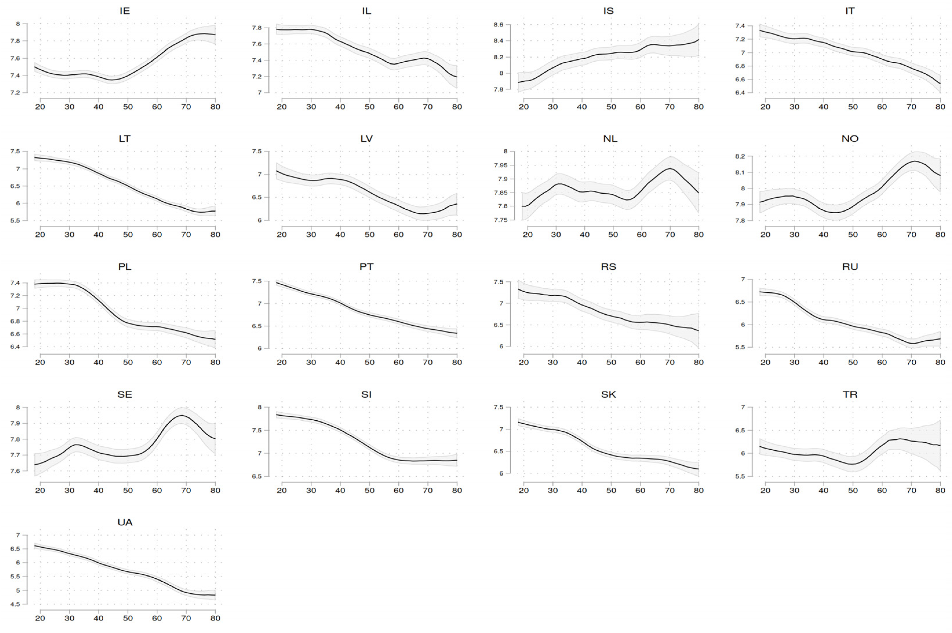

Table A1.
Overview of all relevant statistics by country.
| Country | R² (linear model, %) | R² (cubic model, %) | Log. percentage change linear to cubic | Average happiness | SD overall happiness | Average age | SD age | Happiness range | N |
| AT | 0.093 | 0.128 | 3.628 | 7.573 | 1.915 | 46.629 | 16.695 | 0.242 | 14168 |
| BE | 0.016 | 0.044 | 5.176 | 7.691 | 1.559 | 47.036 | 16.949 | 0.124 | 15946 |
| BG | 7.569 | 7.727 | 0.736 | 5.762 | 2.520 | 48.179 | 16.919 | 2.384 | 12242 |
| CH | 0.082 | 0.154 | 4.485 | 8.086 | 1.480 | 46.646 | 16.624 | 0.230 | 15637 |
| CY | 0.734 | 0.856 | 2.812 | 7.281 | 1.928 | 45.451 | 16.653 | 0.719 | 5614 |
| CZ | 2.096 | 2.121 | 0.183 | 6.882 | 1.915 | 46.346 | 16.567 | 0.894 | 18816 |
| DE | 0.000 | 0.062 | 10.719 | 7.286 | 1.980 | 48.325 | 16.921 | 0.178 | 31224 |
| DK | 0.370 | 0.385 | 1.374 | 8.306 | 1.440 | 46.959 | 16.825 | 0.339 | 11426 |
| EE | 3.731 | 3.926 | 1.656 | 6.976 | 1.942 | 46.481 | 17.192 | 0.958 | 15411 |
| ES | 0.624 | 0.684 | 2.266 | 7.528 | 1.766 | 46.292 | 16.585 | 0.458 | 17934 |
| FI | 0.056 | 0.118 | 4.719 | 8.047 | 1.421 | 47.673 | 16.999 | 0.204 | 17850 |
| FR | 0.874 | 1.071 | 3.118 | 7.273 | 1.780 | 47.200 | 16.855 | 0.500 | 17535 |
| GB | 0.471 | 1.062 | 4.832 | 7.509 | 1.871 | 46.109 | 16.800 | 0.600 | 19134 |
| GR | 2.345 | 2.499 | 1.884 | 6.521 | 2.010 | 47.112 | 16.785 | 1.163 | 11746 |
| HR | 4.686 | 4.778 | 0.671 | 7.189 | 2.143 | 47.692 | 17.353 | 1.667 | 6035 |
| HU | 3.635 | 3.831 | 1.684 | 6.451 | 2.267 | 46.642 | 17.025 | 1.251 | 15480 |
| IE | 0.407 | 0.781 | 4.522 | 7.499 | 1.822 | 43.821 | 16.502 | 0.539 | 20686 |
| IL | 0.832 | 0.834 | -1.183 | 7.595 | 2.008 | 42.467 | 17.128 | 0.594 | 14467 |
| IS | 1.097 | 1.224 | 2.449 | 8.170 | 1.470 | 44.276 | 16.609 | 0.550 | 3653 |
| IT | 1.441 | 1.506 | 1.508 | 7.018 | 1.860 | 48.556 | 17.058 | 0.815 | 9263 |
| LT | 7.096 | 7.240 | 0.702 | 6.575 | 2.109 | 47.439 | 17.014 | 1.590 | 10627 |
| LV | 2.329 | 2.453 | 1.672 | 6.626 | 2.094 | 47.341 | 17.285 | 0.962 | 3577 |
| NL | 0.011 | 0.013 | 2.821 | 7.859 | 1.300 | 46.501 | 16.445 | 0.145 | 17125 |
| NO | 0.174 | 0.286 | 4.154 | 7.960 | 1.562 | 46.162 | 16.564 | 0.328 | 14886 |
| PL | 2.332 | 2.425 | 1.375 | 6.992 | 2.120 | 45.547 | 16.967 | 0.889 | 16076 |
| PT | 3.787 | 3.856 | 0.600 | 6.865 | 1.905 | 47.394 | 17.167 | 1.145 | 16350 |
| RS | 1.360 | 1.369 | -0.419 | 6.852 | 2.421 | 45.810 | 16.104 | 0.996 | 3178 |
| RU | 2.762 | 2.886 | 1.508 | 6.148 | 2.209 | 44.170 | 16.908 | 1.153 | 11554 |
| SE | 0.148 | 0.166 | 2.473 | 7.758 | 1.617 | 46.692 | 16.873 | 0.317 | 16625 |
| SI | 4.238 | 4.554 | 2.009 | 7.286 | 1.940 | 46.754 | 16.810 | 1.010 | 12384 |
| SK | 3.130 | 3.222 | 1.082 | 6.657 | 1.974 | 44.316 | 16.686 | 1.074 | 10492 |
| TR | 0.002 | 0.203 | 9.353 | 6.006 | 2.714 | 40.008 | 15.496 | 0.566 | 3896 |
| UA | 5.686 | 5.688 | -3.188 | 5.826 | 2.367 | 45.119 | 16.963 | 1.790 | 9123 |
Source: ESS1-10. Post-stratification weights applied. ESS round effects are netted out from the R² statistics. Happiness range is the difference between max. and min. values of aggregated happiness over the life course (compare Figure 1). Formulas used: Log. percentage change linear to squared = log[(R² (squared, %)—R² (linear, %)) / R² (linear, %)].
References
- Bartram, D. (2021). Age and Life Satisfaction: Getting Control Variables under Control. Sociology. [CrossRef]
- Bartram, D. (2022). Is Happiness U-Shaped in Age Everywhere? A Methodological Reconsideration for Europe. National Institute Economic Review. [CrossRef]
- Bartram, D. (2024). To Evaluate the Age–Happiness Relationship, Look Beyond Statistical Significance. Journal of Happiness Studies. [CrossRef]
- Becker, C. K. , & Trautmann, S. T. (2022). Does Happiness Increase in Old Age? Longitudinal Evidence from 20 European Countries. Journal of Happiness Studies, 3654. [Google Scholar] [CrossRef]
- Beja, E. L. (2018). The U-shaped relationship between happiness and age: evidence using world values survey data. Quality & Quantity, 1829. [Google Scholar] [CrossRef]
- Bittmann, F. (2021). Beyond the U-Shape: Mapping the Functional Form Between Age and Life Satisfaction for 81 Countries Utilizing a Cluster Procedure. Journal of Happiness Studies, 2343. [Google Scholar] [CrossRef]
- Bittmann, F. (2024). Why do low spirits last? Investigating correlates of cumulative unhappiness using German panel data. Current Psychology. [CrossRef]
- Blanchflower, D. G. , Graham, C., & Piper, A. (2023). Happiness and Age—Resolving the Debate. National Institute Economic Review. [CrossRef]
- Blanchflower, D. G. , & Oswald, A. J. (2009). The U-Shape without Controls. Economic Research Papers. [CrossRef]
- Bryan, J. (1995). Seven Types of Distortion: A Taxonomy of Manipulative Techniques used in Charts and Graphs. Journal of Technical Writing and Communication. [CrossRef]
- Cheng, T. C. , Powdthavee, N., & Oswald, A. J. (2017). Longitudinal Evidence for a Midlife Nadir in Human Well-Being: Results from Four Data Sets. The Economic Journal. [CrossRef]
- Cleveland, W. S. , & Loader, C. (1996). Smoothing by Local Regression: Principles and Methods. In W. Härdle & M. G. Schimek (Eds.), Statistical Theory and Computational Aspects of Smoothing (pp. 10–49). Heidelberg: Physica-Verlag HD. [CrossRef]
- Doherty, A. M. , & Kelly, B. D. (2010). Social and psychological correlates of happiness in 17 European countries. D. ( 27(3), 130–134. [CrossRef]
- Elwert, F. , & Winship, C. (2014). Endogenous Selection Bias: The Problem of Conditioning on a Collider Variable. Annual Review of Sociology. [CrossRef]
- Fan, J. (1992). Design-adaptive Nonparametric Regression. Journal of the American Statistical Association, 1004. [Google Scholar] [CrossRef]
- Graham, C. , & Ruiz Pozuelo, J. (2017). Happiness, stress, and age: how the U curve varies across people and places. Journal of Population Economics. [CrossRef]
- Gujarati, D. N. , & Porter, D. C. (2010). Essentials of econometrics, M: York.
- Haller, M. , & Hadler, M. (2006). How Social Relations and Structures can Produce Happiness and Unhappiness: An International Comparative Analysis. Social Indicators Research. [CrossRef]
- Jebb, A. T. , Morrison, M., Tay, L., & Diener, E. (2020). Subjective Well-Being Around the World: Trends and Predictors Across the Life Span. Psychological Science. [CrossRef]
- Kratz, F. , & Brüderl, J. (2021). The Age Trajectory of Happiness. [CrossRef]
- Mohajeri, K. , Mesgari, M., & Lee, A. S. (2020). When Statistical Significance Is Not Enough: Investigating Relevance, Practical Significance, and Statistical Significance. MIS Quarterly. [CrossRef]
- Wasserstein, R. L. , Schirm, A. L., & Lazar, N. A. (2019). Moving to a World Beyond “ p <0.05.” The American Statistician, 73(sup1), 1–19. 73. [CrossRef]
| 1 | This model contains age, age² and age³ as independent variables. However, note that this decision is somewhat arbitrary and even more complex models might be beneficial for other data or research questions. |
| 2 | This model contains age, age², and age³ as independent variables. |
| 3 | This netting out has been done for all numerical analyses presented in this paper. |
Figure 1.
Graphical comparison of Portugal and Germany using local polynomial smoothing. Two different y-scales applied. Source: ESS1-10. Post-stratification weights applied. 95% CIs included.
Figure 1.
Graphical comparison of Portugal and Germany using local polynomial smoothing. Two different y-scales applied. Source: ESS1-10. Post-stratification weights applied. 95% CIs included.
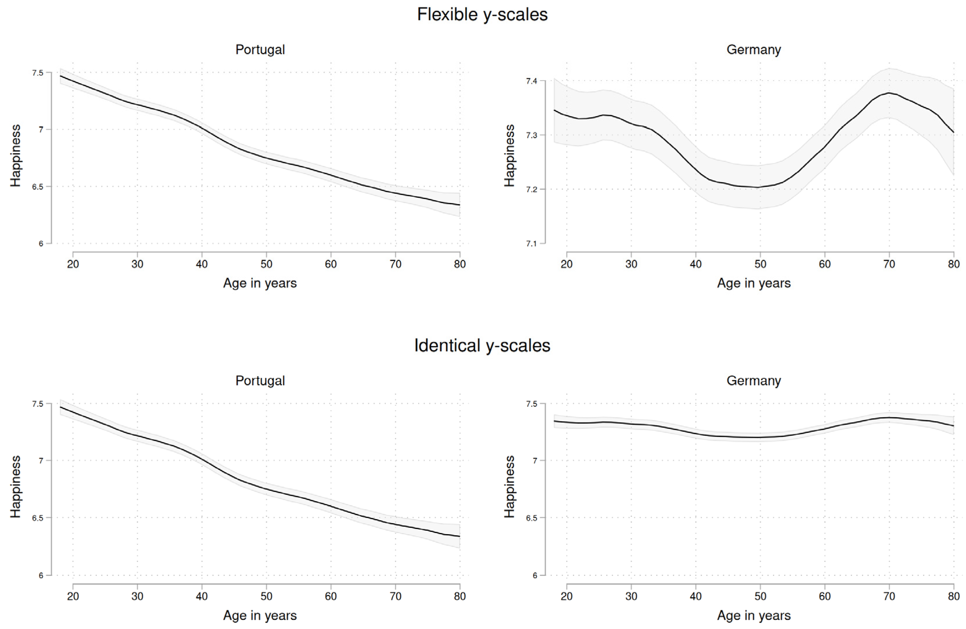
Figure 2.
Overview of key statistics by country. Source: ESS1-10.
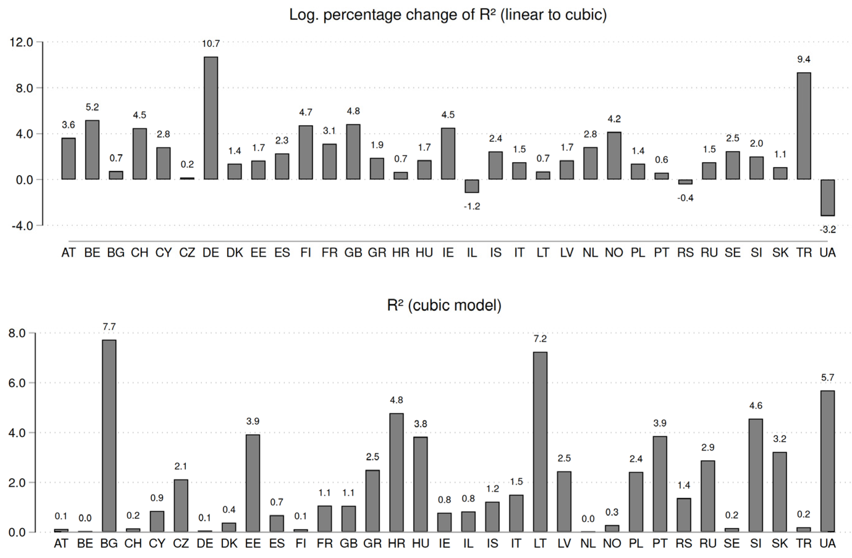
Figure 3.
Scatterplot of total R² and change in R² from a linear to a cubic model by country. Source: ESS1-10. Note the logarithmic scaling of the x-axis. Graphical shape classification is subjective and based on Figure A1 and Figure A2 in the appendix. The higher a numerical value on the x-axis, the less linear the functional form between age and happiness is. The higher a numerical value on the y-axis, the more important age is to explain happiness in general.
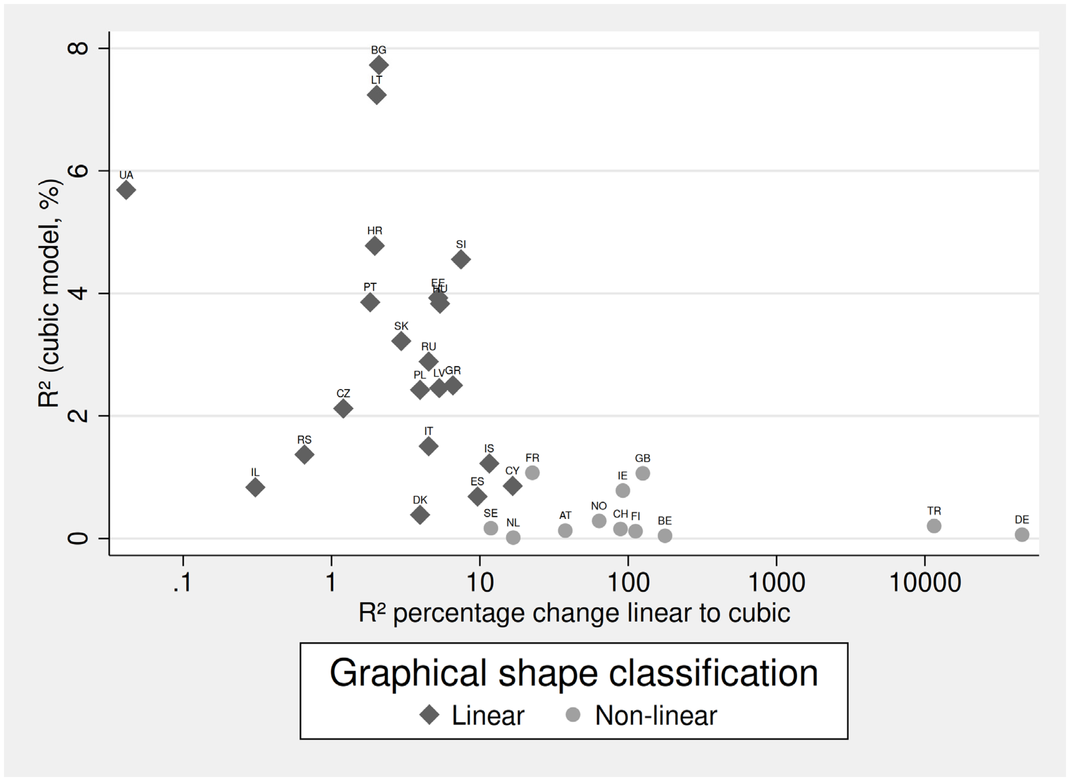
Table 1.
Correlation matrix (Pearson’s r).
| Log. R² change | R² (absolute) | Range of happiness | |
|---|---|---|---|
| Log. R² change | 1 | ||
| R² (absolute, cubic) | -.559*** | 1 | |
| Range of happiness | -.597*** | .941*** | 1 |
Source: ESS1-10. N = 33. *** p < 0.001.
Disclaimer/Publisher’s Note: The statements, opinions and data contained in all publications are solely those of the individual author(s) and contributor(s) and not of MDPI and/or the editor(s). MDPI and/or the editor(s) disclaim responsibility for any injury to people or property resulting from any ideas, methods, instructions or products referred to in the content. |
© 2024 by the authors. Licensee MDPI, Basel, Switzerland. This article is an open access article distributed under the terms and conditions of the Creative Commons Attribution (CC BY) license (https://creativecommons.org/licenses/by/4.0/).
Copyright: This open access article is published under a Creative Commons CC BY 4.0 license, which permit the free download, distribution, and reuse, provided that the author and preprint are cited in any reuse.


