Beyond the Typology: Assessing Urban Fabrics in Cuenca – Ecuador through a Sustainability Lens

Understanding the relationship between urban morphology and sustainability can inform strategies for facing the contemporary challenges of cities since urban fabrics embed information regarding the performance of different urban systems and their spatial heterogeneity. This paper assesses the variability of urban sustainability indicators for urban fabric typologies in Cuenca, Ecuador. We assessed 30 sustainability indicators for each cell in a hexagonal regular grid covering the study area and explored their spatial patterns and relationships with urban fabric typologies through spatial and statistical analysis. Results show that indicators vary significantly among urban fabrics, while built environment indicators dominate overall sustainability levels. A marked spatial heterogeneity is revealed by high sustainability for inner-core areas but much lower sustainability for fringe expansion areas – although transition areas are also identified. Spatial clusters of urban fabrics are found to be homogeneous in terms of sustainability only for urban fabrics with high/low sustainability levels, while heterogenous for fabrics in the mid-range levels. The quantitative evidence on the relation between urban morphology and sustainability unveils otherwise hidden patterns, which can support and enhance evidence-based decision-making for urban planning. Open-source data and tools developed allow full replication for further research in similar urban areas.

Keywords:

Subject:

Social Sciences - Urban Studies and Planning

1. Introduction

Urban sustainability, a widely recognised concept, is often adopted by planners, decision-makers, and politicians as a goal or characteristic of a development model. It is commonly perceived as a quantitative measurement used to compare and rank cities as homogeneous entities. However, it is crucial to challenge this traditional understanding. Cities are the product of complex evolutive processes, where different types of urban fabrics emerge, producing a mosaic of various typologies, each with its own formal and functional characteristics.

Understanding how city sustainability varies among complex urban fabrics within cities does not entail straightforward answers, as cities are the product of inherently complex evolutive processes. Hence, gazing upon cities’ genesis stands as an appropriate starting point.

The roots of land ownership and how it has influenced urbanism can be traced back to ancient times, from the circular house layouts of Natufian dwellings at Ain-Mallaha, 9000 BC, to orthogonal rooms or “Cell-building” at Cayonu, 8000 BC, to the emergence of street patterns in the city of Uruk, circa 3000 BC [1]. Street patterns in urban settlements became the boundaries between public and private property, kept in time by the politics derived from collective ownership [2]. The street is, therefore, the epicentre where human scale is experienced in a city, oscillating between public and private, architectural and urban scales. Several emerging city properties have their roots in the spatial configuration of the streets and buildings, such as the relation between pedestrian volumes and neighbourhood urban form or the imageability and complexity driving urban design features. Moreover, essential streetscape features influencing people’s lives are evidenced at the street level: historic buildings, outdoor dining, active uses, etc. [3].

This paper focuses on intermediate cities (100,000 to 500,000 inhabitants) and Cuenca, Ecuador, as a case study since these are argued to constitute the territories where most of the global urban population lives [4,5]. Intermediate cities are also vital within the “New Urban Agenda” established in Habitat III, being conceived as critical pieces for the achievement of the Sustainable Development Goals (SDG) [6].

A comprehensive measurement of cities’ sustainability should incorporate life-quality issues such as (dis)satisfaction with city life [7], urban imbalance and segregation [8,9], changing paradigms and policies [10], among others. Consequently, a methodological approach widely employed in urban contexts is creating urban sustainability indicators (USIs) [11], ranging from environmental and economic sustainability to equity and environmental justice at the city scale. Withal, SIs can be profoundly understood through what has been described as “strong sustainability” [12], which is focused on “increasing the efficiency of resource consumption; (ii) harvesting renewable resources limited by their regeneration rates; (iii) reducing greenhouse gas emissions; (iv) reusing wastes as input in other processes; (v) replacing toxic inputs with organic ones; (vi) replacing energy from non-renewable sources with that from renewable ones; (vii) increasing affordability; and (viii) increasing sustainable manufacturing” [12]. While the field has advanced in recent years, an over-attention to environmental aspects has been identified in the literature at the expense of socio-economic elements [13]. Cities are complex systems that result from adapting the natural environment to human conditions; as such, they display metabolic processes (production, consumption, and waste) analogous to the observable function of biological organisms within their ecosystems [14]. Henceforth, managing cities as urban organisms in a sustainable and regenerative manner requires solutions that address the specific metabolic type of each city, seeking to “reduce its metabolic footprint (resource inputs and waste outputs) whilst improving its liveability” [11].

Urban research employing indicators has been conducted extensively on several domains. It must be noted, however, that the primary trend worldwide for measuring urban sustainability considers the city as a unique, homogenous body, computing aggregate city-wide indicators, thus disregarding spatial variability and the intrinsic heterogeneity of urban systems [15]. Some notable exceptions exist in the most recent literature, varying in spatial disaggregation and indicator specificity. In a study focused on resilience [16], a set of 42 indicators for the Madrid region are mapped to socio-cultural, economic, ecological, physical and technological, and governance system dimensions, yet at a high spatial aggregation at the level of municipalities, whereby the smallest unit is 5 km², and the largest is 605.77 km². Another study focused on urban vitality in Nanjing [17], a set of 71 indicators mapped to social, economic, cyberspace, and cultural-tourism dimensions, whereby a cellular automata grid of 500m rectangular blocks determines the level of spatial disaggregation. While several parallels exist among vitality, resilience, and sustainability, these cannot be considered equivalent, with sustainability being a broader, more encompassing concept. Finally, research explicitly focused on urban sustainability also exists [18], yet a relatively high spatial granularity level is set at Chinese cities/prefectures, while indicators are established directly at 12 high-level dimensions – as opposed to the studies referenced thus far, which have a lower layer of various specific indicators mapped to an upper high-level layer of dimensions. To address the argued limitations in the literature, the approach adopted for this paper relies on a spatially disaggregate characterisation of USIs, whereby the study area is discretised by a spatial grid with observational units consisting of 150m-radius hexagons.

A second fundamental methodological pillar of this paper aims to generate sustainable indicators applicable to a human scale, that is, spatial units that a person can recognise and relate to in their daily life, generating sustainable indicators applicable to a human scale and ensuring that the metrics can ultimately be directed towards improving the quality of life of all inhabitants of a city [15]. An appropriate scale for this endeavour can be found in urban fabrics, which can be defined as confined city areas that present similar morphological characteristics, able to influence people’s experience and behaviour in aspects such as perception of space, commuting decisions, purchases and consumption, as well as the environmental performance of a place [19]. Urban fabrics have been classified by Wheeler [19] into 27 types of “built landscapes”, defined as an “area of consistent form at a neighbourhood scale, often 1 square km or greater. This is an area large enough to determine much of a resident or user’s daily experience and has a significant influence on shaping resident behaviour” ([19], p. 167). However, urban fabrics themselves cannot inform about sustainability, at least not directly or explicitly; hence, this paper aims to go beyond the typology and confer a sustainability meaning to urban fabrics. Connecting these two fundamental urban aspects can be instrumental in improving cities and the quality of life through urban planning. Additionally, focusing on an urban fabrics scale with a granularity of 150m-radius hexagons allows reaching the neighbourhood and citizen scale, thus addressing the limitations of USIs calculated at the aggregate city level – which would not correctly capture cities’ heterogeneity.

All considered, cities’ spatial (land distribution) and functional aspects (urban fabrics and population behaviour) are a source of considerable heterogeneity, which requires an appropriate scale to account for the differentiated flux of matter, energy, and waste of distinct parts of the city, and fully understand the urban metabolism of a city [15]. This approach is essential in the context of Latin American cities as well to reveal sustainability inequalities, considering that the region ranks as the most unequal in the world [20]. The contribution of this paper concerning the existing body of research in urban sustainability studies reported above consists of a first-of-its-kind assessment of the relationship among urban sustainability indicators and urban fabric typologies at a mesoscale (neighbourhood level of disaggregation, applied for city-wide analyses), taking the case study of the intermediate city of Cuenca, in the southern Andes region of Ecuador. Among the main findings, evidence suggests that built environment indicators present significant variation among urban fabrics, dominating city-wide sustainability levels. A marked spatial heterogeneity is also revealed, with high sustainability for inner-core areas but much lower sustainability for fringe expansion areas – although transition areas are also identified. Spatial clusters of urban fabrics are found to be homogeneous in terms of sustainability only for urban fabrics with high/low sustainability levels, while heterogenous for fabrics in the mid-range levels. Such findings’ implications and significance are instrumental in urban planning and decision-making processes, as they offer quantitative evidence that can shape spatially-sensitive, equity-based interventions.

2. Methods

This section describes the study area, the available input data for the analyses, and the statistical methods, visualisation techniques and GIS tools deployed for analyses.

2.1. Study Area

Cuenca is an intermediate city located in the southern Andes region of Ecuador at 2550 m.a.s.l.; its territory is geologically divided into three natural terraces marked by the Tomebamba and Yanuncay rivers. Founded by Spain in 1557, Cuenca´s urban layout followed the laws of the Indies and thus adopted the checkerboard grid still present in its downtown area. Since the 1950s, the city has experienced accelerated growth and currently is the third most populated city in Ecuador. Some key characteristics of the city are reported in Table 1 below.

As a newly induced Habitat III intermediate city, back in 2015, Cuenca embarked on a more robust pursuit of Sustainable Development Goals (SDG) [21], particularly SDG11: “Make cities and human settlements inclusive, safe, resilient and sustainable”. This unveiled an urgent need for a formal measurement of sustainability, encouraging diverse studies around the field for the city.

The city of Cuenca offers potential transferability within the region, as it displays a heterogeneous urban morphology representative of modern expansions of Latin American intermediate cities [22,23]. The next subsection briefly describes a characterisation of Cuenca´s urban morphology into urban fabric typologies.

2.2. Data

Following the argument supporting a vision of strong sustainability that addresses life-quality issues and metabolic processes of cities, a comprehensive set of indicators has been previously calculated for the city of Cuenca [22] under the assumption of a compact city model. The original set comprised 58 indicators at a conceptual level, yet full data exists for only 37 of them, and some additions have also been conducted for this study with respect to [22]. The updated set of indicators can be grouped into four higher-level dimensions: a) Built Environment, b) Biophysical Environment, c) Urban Systems, and d) Socio-Spatial Dynamics (Table 2). These indicators are stored in a geographic information systems layer2, spatially disaggregated by a regular grid with hexagons of 150m radius.

A quick exploratory data analysis revealed that several USIs had all values 100% (B1 and C13) or 0% (A7, A9, B3, C4, and C8). While these are extreme values with crucial practical significance, this study aims to assess differential patterns rather than overall sustainability magnitudes. Hence, these indicators are removed from consideration, leaving 30 USIs for the analyses.

The second key data source consists of a typology of urban fabrics, which has already been defined in previous research for the whole city of Cuenca [25], following the approach suggested by Wheeler [19] and adapting it to the local context. It is important to note that four rivers – Tomebamba, Tarqui, Yanuncay y Machángara – traverse the city and contribute to green areas of great importance; however, these typologies have been removed from the study since they do not represent populated areas and therefore, most indicators are not relevant [25]. Eighteen UFTs result from the adaptation to Cuenca, seventeen of which fall within urban boundaries (Figure 1). For a detailed description of each typology, see [25]. A GIS layer3 with the identified UFTs is openly available.

Some cells located at the fringe of the study area are labelled as UNCLASSIFIED. Considering that these cells are predominantly located in expansion areas, they were kept for analysis, as they can offer important insights regarding the sustainability of city expansion areas.

2.3. Methods and Analyses

The approach proposed in this paper aims to explore the relationship between urban fabric typologies (UFTs) and urban sustainability indicators (USIs) through data visualisation techniques, geospatial analyses, and statistical analyses. Both data sources utilised (UFTs and USIs) are spatially disaggregated by the same 150m-radius hexagonal grid, granting a one-to-one mapping that eliminates the occurrence of spatial overlapping mismatches; the hexagonal grid approach also offers a workaround to avoid the modifiable areal unit problem [26].

Two statistical tests are conducted at a pre-analysis step. First, 30 individual one-way ANOVA tests are conducted for each USI to assess whether there is a statistical variation of sustainability indicators for the 18 UFTs present in Cuenca. In other words, answering this question provides evidence that if we obtain the means of each USI grouped by each UFT, these are significantly different among themselves. Note that spatial patterns are already considered implicitly in this analysis because, for every USI, the mean values of each UFT category correspond to averaging the values of all hexagonal cells of that category across the study area.

For the second pre-step, a Principal Component Analysis (PCA) is deemed necessary considering the high dimensionality involved in the study layout – having 30 USIs, each analysed against 18 UFTs. An important question to answer is whether each of the 30 USIs is pertinent in adding unique information and variability with respect to the rest. PCA is thus conducted to assess the degree to which the 30 USIs are correlated and whether it is pertinent to transform them into a lower dimensional array through linear transformations.

In-depth analyses begin with data analysis and visualisation to assess how sustainability varies for UFTs at a more comprehensive level, which consists of aggregating USIs into an overall multicriteria sustainability metric. To delve further into this exploration, an overall sustainability index is computed as follows:

Outliers for each USI are treated first based on the following criteria:

$L o w e r l i m i t = 1 s t q u a r t i l e - 1.5 * I Q R$

$U p p e r l i m i t = 3 r d q u a r t i l e + 1.5 * I Q R$

$I Q R = 3 r d q u a r t i l e - 1 s t q u a r t i l e$

All values beyond the limits are truncated at the limit value.
Then, each USI is normalised against its maximum value (upper limit, after truncation) in the [0, 1] domain. Note that this normalisation process is chosen instead of Z-scores, as centring values around zero would be inadequate for adding sustainability to all USIs.
The overall sustainability index consists of a linear combination (algebraic sum) of the 30 normalised USIs.

○

Note that some USIs are defined negatively regarding sustainability (e.g., unemployment). Hence, they enter the algebraic sum with a negative sign. The negative USIs are: A5, A10, D2, D3, D9, D11, D15, and D16. The logic is simple: Since they are negatively defined, the magnitude of a given negative USI (their ideal values being zero) reduces overall sustainability.

○

D17 is a particular case since its construction sets its optimal value as 1, and sustainability decreases both for values greater than 1 and lower than 1. Thus, the normalisation for this index consists of recentring it around zero (subtracting 1 from all values) and then converting negative values to absolute positive values. The normalised version of D17 measures a bidirectional distance from the optimal value.

It must be noted that the overall sustainability index’s purpose is to establish a common metric to enable formal comparison and differential analysis; hence, the magnitude of this index’s values is not subject to analysis or interpretation in this study. This is also in line with the rationale mentioned in section 2.2 for removing USIs with all-100 or all-0 values.

Existing indicator-based studies argue that individual indicators may capture more than one attribute and propose adding specific weight coefficients at the level of high-level dimensions [16]. In this sense, an essential application of the PCA pre-step mentioned above is also assessing whether weighting is necessary, depending on how well-differentiated (or not) USIs are regarding the information they provide.

Based on the proposed index, the following visualisation techniques, statistical tests, and spatial analyses are conducted:

A faceted boxplot of the overall sustainability index values for each urban fabric typology to reveal intra- and inter-class patterns. This visualisation offers a first insight into more/less sustainable UFTs and more/less variable UFTs.
An ANOVA test contrasting the overall sustainability index with UFTs, accompanied by Tukey’s Honest Significant Differences test, to test whether UFTs significantly differ among themselves, assessing pairwise combinations.
A natural question that follows the preceding analyses is whether the identified (dis)similarities are due to cells being spatially clustered in specific or are unrelated to location. This question can be answered using choropleth maps to unveil spatial patterns of UTF’s overall sustainability. Understanding whether high/low sustainability UFTs or high/low variation UFTs are spatially concentrated or randomly spread out throughout the city becomes fundamental. Despite Figure 1 already showing spatial concentrations of UFTs in certain areas, this does not necessarily imply that cells within a UFT cluster are also similar in sustainability.

All spatial analyses are conducted in QGIS 3.344, while statistical analyses and visualisation are performed in R Statistical Software5.

3. Results

This section reports four key findings: a statistically significant variability of USIs concerning UFTs; proof that the set of USIs is pertinent and non-redundant; data visualisation and statistical analyses evidencing heterogeneity of UFTs in terms of sustainability levels; and choropleth maps unveiling distinct spatial sustainability patterns of UFTs.

3.1. One-way ANOVA tests

All 30 ANOVA tests were satisfactory, meaning that the null hypothesis of no statistically significant variation of each USI with respect to all UFT levels cannot be rejected. All tests yield p-values of practically 0, implying high statistical significance. Results are shown in Table 3 below.

These tests offer first-order evidence justifying further analyses on the premise that statistically significant spatial heterogeneity exists in the data, considering the abovementioned argument that spatial patterns are implicit in the hexagonal analysis units.

3.2. Principal Component Analysis

A different variable normalisation process is performed to conduct PCA, whereby USI variables are normalised as Z-scores – subtracting their mean and dividing by their standard deviation. A correlation plot is also helpful in gaining an initial perspective on the potential for dimensionality reduction. Figure 2 below suggests that correlation is generally low, with some variables showing an expected moderate correlation due to their conceptual definition – e.g., A8-Proximity to open public spaces and B4-Proximity to green spaces.

PCA is then applied to the data in R, yielding principal components, understood as linear transformations and combinations of the original USI variables. The next step is assessing the importance (relevance) of each principal component, which can be visualised by a scree plot generated with the factoextra R package6. Figure 3 below shows the top 10 components in terms of the percentage of variance they explain (all remaining 20 components explain less than 3% of variance each).

The results from the scree plot suggest that the linear transformations undertaken in the PCA procedure do not offer a justifiable reduction in dimensionality since the first principal component only captures 28% of the variance and the remaining components display an exponential decay pattern in variance explained. Not even 50% of the variance is explained among the four best principal components. All considered, it is evidenced that all USIs offer well-differentiated information, and it is best to maintain them all in their original form; furthermore, these results support the decision of constructing the overall sustainability index as a non-weighted linear combination of USIs (all with the same weight of 1).

3.3. Data Visualisation and Statistical Analyses

The results in section 3.1 confirmed statistically significant variation of individual USIs among UFTs, but sustainability cannot be defined solely by one USI or another; more meaningful results must consider the overall sustainability index proposed.

Building on this overall sustainability index, a key question sought in this study can be answered: are some UFTs in Cuenca more sustainable than others? The boxplot depicted in Figure 4 below demonstrates distinct sustainability levels in Cuenca, depending on the urban fabric typology.

In general, it becomes clear from Figure 4 that considerable variation exists in the overall sustainability levels of UFTs. While several contrasts can be made, the most interesting ones are arguably found in analysing extremes. Notably, the average overall sustainability of the Rectangular Block Grid typology is around twice that of the Allotment Gardens typology (Apartment Blocks typology is even higher, yet has too few observations). Further, boxplots also convey important differences regarding intra-class variability, the highest being UpscEnclaveslave, Heavy Industry, and Garden Apartments. At the same time, the lowest is Urban Grid (again, UFTs with a low number of observations are not considered). In other words, Urban Grid cells are much more homogeneous in terms of overall sustainability than their counterparts.

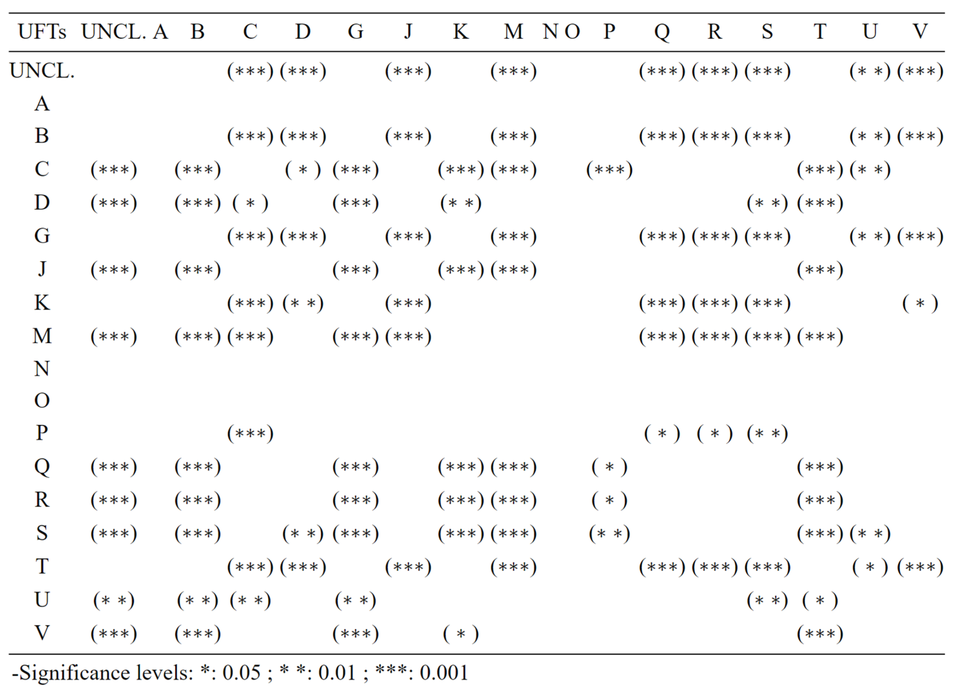
The results from statistical analyses are reported next to complement the findings obtained from visualisation techniques. An initial ANOVA test expectedly yielded a significant p-value (≈0), and results from Tukey’s Honest Significant Differences pairwise combinations are shown in Table 4.

The results shown in Table 4 show that every UFT category is significantly different from at least five other categories and, at most, nine categories. Expectedly, UFTs A, N, O, and P do not have statistically significant results due to their low number of observations. Nonetheless, these results further prove that heterogeneity and significant differences in sustainability exist at pairwise UFT levels.

Finally, note that the results for the UNCLASSIFIED UFT in Table 4, along with the results in Figure 4, fully justify including UNCLASSIFIED cells for the analysis, as these show a distinct low sustainability pattern and vary significantly for most UFTs.

3.4. Spatial Analyses

The analyses conducted thus far have demonstrated statistically significant heterogeneity among UFTs at different levels of aggregation and measured by a synthetic index of overall sustainability. Following both research and practical urban planning interests, it is important to understand whether UFT clusters are homogeneous or heterogeneous in terms of overall sustainability levels, and conversely, whether high/low sustainability areas display specific UFT patterns.

Figure 5 presents a choropleth map of Cuenca discretized spatially by the 150m-radius hexagonal grid proposed in this study. A viridis colour scale characterises the overall sustainability index, while text labels overlaid to each hexagonal cell report its urban fabric typology.

Upon inspection, it can be evidenced that some urban fabric clusters are indeed similar in their sustainability levels, while others are more spread out and heterogeneous. The first well-defined spatial pattern can be located towards the south of the city, consisting of a high-sustainability cluster formed by Q: Organic, R: Quasi-Grid, and S: Rectangular Block Grid UFTs. These three fabrics are also less concentrated in the city’s central- and south-western areas, always showing high sustainability. Interestingly, the S fabric also emerges as an “oasis” of high sustainability amid a very low sustainable area towards the northern-central region of the city.

Exploring the lower end of the sustainability spectrum, an expected spatial pattern can be evidenced towards the north, south, east, and, to a lesser degree, towards the west. In these expansion areas, a considerable degree of spatial proximity (clustering) emerges, whereby predominant UFTs are B: Allotment Gardens, G: Country Roads, K: Heavy Industry, T: Rural Sprawl, and Unclassified.

The contrast between high and low sustainability areas (the two highest vs. the two lowest ranges of the overall index) can be better visualised in Figure 6 below. These areas are spatially mutually exclusive, except for the “oasis” identified earlier. Thus, evidence suggests that, for high/low sustainability values, spatial clusters also implied homogeneity in the sustainability levels.

Another informative choropleth map is shown in Figure 7, where an interesting pattern can be spotted regarding expansion areas of the city; seen together with Figure 6, appear to have transitioning areas or clusters of typically low-performing UFTs (B, T, K, and G), with better sustainability levels than their surroundings. In general, however, Figure 7 suggests that mid-range sustainability cells are distributed somewhat evenly along the study area – except for the high sustainability cluster in the south of the city.

Consider the information in Figure 4, where J: Garden Apartments is the UFT with the highest intra-class variability. In Figure 7 and Figure 8, specific areas where the J UFT is clustered can be identified; interestingly, some of these clusters also show variation in overall sustainability levels. These patterns confirm the intra-class variability found in the statistical analyses but, more importantly, demonstrate that spatial clustering does not necessarily imply homogeneity in terms of sustainability for the mid-ranges of overall sustainability.

A final question deemed worth exploring within the scope of this paper is concerned with aggregation: to which extent patterns are hidden by aggregating all USIs into an overall synthetic index; in other words, to which extent certain USIs may illuminate or obscure overall patterns. To answer this question, the same spatial analyses are now conducted at the level of the four higher-level sustainability dimensions: a) Built Environment, b) Biophysical Environment, c) Urban Systems, and d) Socio-Spatial Dynamics. This level of aggregation is a good trade-off between complete aggregation (overall index) and complete disaggregation (individual USIs). Figure 8 shows the spatial patterns of each dimension.

It is important to note that, at this level of aggregation, the range of sustainability values differs from the one utilised for overall sustainability in previous figures; hence, Figure 6 should not be compared directly to previous figures. Moreover, a new scale with a unified range is set for Figure 8 to provide an unbiased comparative standpoint among the four dimensions. Also note that negative values now appear at the lower end of the new scale, which means that, for some cells, the negatively defined USIs outweigh their positively defined counterparts. Regardless, the reader is reminded that index magnitudes are not the focus of this study, only patterns and comparative differences. Finally, UFT labels have been removed because the focus now is not on UFT patterns but on the differential influence of dimensions in the overall index.

A simple inspection of Figure 8 fully validates the expected loss of variability due to aggregation. Clearly, the spatial patterns and heterogeneity observed in Dimension A: Built Environment resemble the ones for overall sustainability, demonstrating that this dimension dominates the others. Dimension B: Biophysical Environment captures variations in sustainability between inner-core and outer expansion areas of the city– although this is better captured by Dimension A. Moreover, Dimension C: Urban Systems is mostly homogeneous with mid-range sustainability values, capturing minimal variability. Finally, Dimension D displays considerable variability, which somewhat resembles the patterns found in the overall sustainability choropleth map, yet with a much narrower range of sustainability ([1.42, 11.95] for the overall graph vs. [≈0, 5.6] for Dimension D). All considered, Dimension A dominates overall sustainability patterns.

4. Discussion

As an initial important point of clarification, it should be acknowledged that USIs have been constructed to measure urban sustainability, intrinsically neglecting measures of sustainability in rurality. Nevertheless, these distinctions can become difficult to ascertain, as in the case of Cuenca, fundamentally rural fabrics fall within the limits of what is considered the urban area, adding up to 33.63% of all fabrics (Rural Sprawl, Incremental Mixed and Country Roads).

The findings reported in Section 3 unveil otherwise hidden patterns, which, beyond their scientific value, are particularly useful for urban planners for several reasons. First, identifying a ranking of UFTs in terms of their sustainability confirms/denies prior judgement-based conceptions, formalising discussions, analyses, and decision-making processes. Formulation of urban interventions (in the short to medium term) and urban planning strategies (in the medium to long term) can incorporate quantitative evidence on the sustainability of different urban fabrics.

Second, distinct spatial heterogeneity is revealed. Some of this heterogeneity is an expected, confirmatory result, such as high sustainability levels for inner-core areas but much lower sustainability for fringe expansion areas. However, some heterogeneity emerges upon disaggregation and spatial mapping, such as transition “mini-clusters” with higher sustainability amid fringe expansion areas. These transition areas can prove instrumental in planning and policymaking, as they allow the identification of UFTs that are conducive to higher sustainability in expansion areas.

Third, an interesting non-linear pattern of spatial heterogeneity is unveiled. Spatial clusters of urban fabrics are found to be mainly homogeneous in terms of sustainability, only for urban fabrics with high/low sustainability levels. At the same time, they are mostly heterogeneous for fabrics in the mid-range levels. This result can be postulated as a cautionary finding because it cannot be assumed that spatially clustered UFTs (same type) will have similar sustainability levels. In the case of Cuenca, this is only true for extreme values.

Fourth, results from the analyses at a level of disaggregation of high-level sustainability dimensions offer key insights into the city’s performance in these areas. Note that, from a purely data analysis perspective, this paper reports that Dimension A: Built Environment dominates overall patterns, yet Figure 8 shows that this dimension is arguably the most unequal from a practical standpoint. On the same logic, it can be argued that the city is performing quite well regarding Dimension D: Socio-Spatial Integration in terms of sustainability and equity.

Fifth, while the scale of this study is at the city level, the spatial disaggregation by hexagonal cells enables analyses at the parish level or specific zones of interest. For instance, the westernmost expansion area of the city shows considerable variability among high-level dimensions, which might warrant a more profound investigation for focused interventions.

Among the most relevant limitations of this study, the authors would like to acknowledge the following: 1) While data-gathering efforts were quite extensive back in 2018, several indicators from the original set of 58 could not be gathered due to time and economic constraints. Hence, a data actualisation effort would be completed, and the set of indicators would be updated periodically to reflect the temporal variation. 2) While the criteria for removing the four rivers traversing the city of Cuenca is justified in [25], it has an impact on the sustainability indicators values, particularly in terms of Dimension B: Biophysical Environment. As this study focuses on the relationship to urban fabric typologies, we suggest not using the values reported here for this dimension but rather referring to the original dataset. 3) A non-weighted linear combination of indicators currently constructs the overall sustainability index; however, an enhancement would consider differential impacts of indicators or high-level dimensions by applying specific weights.

The research group developed an open-access tool available as a QGIS plug-in named MESUE7, with specific functionality to allow exploration and customisation of USIs weights. While this can be easily constructed as a “sandbox” exercise for practical scenario-exploration purposes, the challenge from a rigorous scientific standpoint is establishing these weights from ground truth data – currently inexistent and undefined.

In addition to addressing the abovementioned limitations, future work can be conceived in two key areas. First, increasing the complexity of analysis methods by employing econometric models on the branch of logistic regression, which would adjust to the categorical-quantitative nature of the data (UFTs-USIs), and they would allow to further formalise relations and effects among UFTs and USIs at a fully disaggregate level. Second, an exciting research avenue would involve deploying the approach proposed in this paper in other intermediate cities in the Andes and Latin America. Such efforts would allow identifying similarities and differences among case studies, and the authors expect that a considerable generalisation potential may exist among similar cities.

5. Conclusions

The results reported in Section 3 of this paper confirm its main hypothesis since they provide conclusive evidence that not only urban fabric typologies display distinct sustainability patterns in their spatial distribution but also among and within themselves – inter- and intra-class variability. This evidence is further supported by statistical tests demonstrating significant variability and differences, both at aggregate and disaggregate levels.

Further, the spatial patterns identified provide an understanding of macro-level city sustainability computed from micro-level analysis units (cells capturing the neighbourhood scale). This is particularly important to overcome aggregation limitations in current city-wide sustainability metrics. The macro-level sustainability picture allows to identify distinct patterns of core and expansion areas, while relating these to urban fabric patterns.

The contributions of this paper are novel in terms of the level of disaggregation achieved, the comprehensiveness and completeness of the set of USIs, and, more importantly, since UTFs evolve from a mere characterisation of morphology to a metric embedded with sustainability meaning. Nevertheless, findings from this paper also bring forth new questions regarding the drivers behind spatial and data patterns, which may arise from urban planning practices, municipal regulation, and even socioeconomic attributes of the population (if people´s location choices, as well as private real estate investment, are considered). Consequently, the research avenues proposed for future work focused on econometric modelling and transferring the approach to similar case studies offer great potential for delving further into these new questions.

As a contribution to the state-of-the-practice, several application areas are discussed in Section 4 of this paper, which outlines how the findings reported can be applied to enhance and better inform urban interventions, urban planning, policy and regulation, and decision-making processes. It is precisely in this area of application where improvements in city sustainability can be pursued, building up from grounded data and formal analyses.

Finally, it is worth mentioning that the open-source data and tools developed enhance conditions for utilising this paper’s contributions, for academics, practitioners, and decision-makers.

Author Contributions

Conceptualization, Francisco Calderón, Daniel Orellana and Maria Augusta Hermida; methodology, Francisco Calderón, Daniel Orellana, Maria Isabel Carrasco, Johnatan Astudillo, and Maria Augusta Hermida; software, Francisco Calderón, and Johnatan Astudillo; formal analysis, Francisco Calderón, and Daniel Orellana; investigation, Francisco Calderón, Daniel Orellana, Maria Isabel Carrasco, Johnatan Astudillo and Maria Augusta Hermida; data curation, and visualisation, Francisco Calderón; writing—original draft preparation, Francisco Calderón, Daniel Orellana, Maria Isabel Carrasco, and Maria Augusta Hermida; writing—review and editing, Francisco Calderón and Daniel Orellana; supervision, project administration, funding, and funding acquisition, Daniel Orellana and Maria Augusta Hermida. All authors have read and agreed to the published version of the manuscript.

Funding

This research is part of the project “Evaluación de sustentabilidad en tejidos urbanos: Sistema de Indicadores y herramienta de análisis espacial (SISURBANO)”, funded by Dirección de Investigación de la Universidad de Cuenca. The APC was funded by Vicerrectorado de Investigación de la Universidad de Cuenca.

Data Availability Statement

The original data presented in the study are openly available at the GeoLlactaLAB web repository: http://201.159.223.152.

Acknowledgments

We express our gratitude to the institutions that facilitated the access to the data for this research, including the GAD Municipal de Cuenca, Municipal Corporation, ETAPA, EMOV-EP, and Empresa Eléctrica Centro Sur. We are also grateful to technicians and experts who provided insights and feedback on the conceptualisation of sustainability indicators. Finally, we want to recognise the efforts of researchers at LlactaLAB UCuenca, in particular to research assistants and undergrad students who participated in the data collection and processing.

Conflicts of Interest

The authors declare no conflicts of interest. The funders had no role in the design of the study; in the collection, analyses, or interpretation of data; in the writing of the manuscript; or in the decision to publish the results.

References

Aureli, P.; Turan, N. [Re]Form: New Investigations in Urban Form, Panel 1. Harvard GSD 2018. https://youtu.be/0L7Anlsu2A4.
Doug Allen Institute. Streets Lecture - Part 1 2016. https://www.youtube.com/watch?v=NA2jpARqS7A&feature=youtu.be.
Park, K.; Ewing, R.; Sabouri, S.; Larsen, J. Street life and the built environment in an auto-oriented US region. Cities 2019, 88, 243–251. [Google Scholar] [CrossRef]
González, L.G.; Siavichay, E.; Espinoza, J.L. Impact of EV fast charging stations on the power distribution network of a Latin American intermediate city. Renewable and Sustainable Energy Reviews 2019, 107, 309–318. [Google Scholar] [CrossRef]
Mackay, H. Mapping and characterising the urban agricultural landscape of two intermediate-sized Ghanaian cities. Land Use Policy 2018, 70, 182–197. [Google Scholar] [CrossRef]
United Nations. The New Urban Agenda; United Nations: Quito, Ecuador, 2017; ISBN 978-92-1-132731-1. [Google Scholar]
Valente, R.; Berry, B. Dissatisfaction with city life? Latin America revisited. Cities 2016, 50, 62–67. [Google Scholar] [CrossRef]
Garcia-Ayllon, S. Rapid development as a factor of imbalance in urban growth of cities in Latin America: A perspective based on territorial indicators. Habitat International 2016, 58, 127–142. [Google Scholar] [CrossRef]
Smets, P.; Salman, T. The multi-layered-ness of urban segregation. On the simultaneous inclusion and exclusion in Latin American cities. Habitat International 2016, 54, 80–87. [Google Scholar] [CrossRef]
van Lindert, P. Rethinking urban development in Latin America: A review of changing paradigms and policies. Habitat International 2016, 54, 253–264. [Google Scholar] [CrossRef]
Thomson, G.; Newman, P. Urban fabrics and urban metabolism – from sustainable to regenerative cities. Resources, Conservation and Recycling 2018, 132, 218–229. [Google Scholar] [CrossRef]
De Oliveira Neto, G.; Pinto, L.; Giannetti, A.; de Almeida, C. A framework of actions for strong sustainability. Journal of Cleaner Production 2018, 196, 1629–1643. [Google Scholar] [CrossRef]
Sharifi, A. Urban sustainability assessment: An overview and bibliometric analysis. Ecological Indicators 2021, 121. [Google Scholar] [CrossRef]
Rojas, F.; Borthagaray, A.; Marques, A.; Chong, J.; Strobel, J.; Bonilla, L.; Mondino, M.; Pineda, M.; Ellinger, P.; Carrasco, P.; Nemirovsky, Y. La ciudad como sistema: metabolismo, resiliencia y sustentabilidad. Ediciones Irradia. Disruptiva. 2023; 1ª ed. ISBN 978-987-48044-3-3.
Verma, P.; Raghubanshi, A. Urban sustainability indicators: Challenges and opportunities. Ecological Indicators 2018, 93, 282–291. [Google Scholar] [CrossRef]
Suárez, M.; Benayas, J.; Justel, A.; Sisto, R.; Montes, C.; Sanz-Casado, E. A holistic index-based framework to assess urban resilience: Application to the Madrid Region, Spain. Ecological Indicators 2024, 166. [Google Scholar] [CrossRef]
Wang, Z.; Wang, X.; Liu, Y.; Zhu, L. Identification of 71 factors influencing urban vitality and examination of their spatial dependence: A comprehensive validation applying multiple machine-learning models. Sustainable Cities and Society 2024, 108. [Google Scholar] [CrossRef]
Wang, C.; Quan, Y.; Li, X.; Yan, Y.; Zhang, J.; Song, W.; Lu, J.; Wu, G. Characterizing and analyzing the sustainability and potential of China’s cities over the past three decades. Ecological Indicators 2022, 136. [Google Scholar] [CrossRef]
Wheeler, S. Built Landscapes of Metropolitan Regions: An International Typology. Journal of the American Planning Association 2015, 81, 167–190. [Google Scholar] [CrossRef]
Programa de las Naciones Unidas para los Asentamientos Humanos. Construcción de Ciudades más Equitativas, Políticas públicas para la inclusión en América Latina; United Nations: Nairobi, Kenia, 2014; ISBN 978-92-1-132605-5. [Google Scholar]
United Nations Cuenca Declaration for Habitat III “Intermediate Cities: Urban Growth and Renewal”. Available online: http://habitat3.org/wp-content/uploads/Declaration-Cuenca.pdf (accessed on 17 October 2019).
Hermida, M.; Calle, C.; Cabrera, N. La ciudad empieza aquí: metodología para la construcción de barrios compactos sustentables; Universidad de Cuenca: Cuenca, Ecuador, 2015; ISBN 978-9978-14-318-6. [Google Scholar]
Cabrera, N.; Hermida, M. , Orellana, D., Osorio, P. Assessing the sustainability of urban density. Indicators in the case of Cuenca (Ecuador). Bitácora Urbano Territorial 2015, 25. [Google Scholar] [CrossRef]
Shannon, C.; Weaver, W. The mathematical theory of communication; The University of Illinois Press: Urbana, 1964; Volume 14, pp. 306–317. Available online: https://www.ncbi.nlm.nih.gov/pubmed/9230594.
Hermida, M.; Cobo, D.; Neira, C. Challenges and Opportunities of Urban Fabrics for Sustainable Planning In Cuenca (Ecuador). IOP Conference Series: Earth and Environmental Science 2019, 290. [Google Scholar] [CrossRef]
Openshaw, S. The modifiable areal unit problem; OCLC 12052482; Geo Books: Norwick, 1983; ISBN 0860941345. [Google Scholar]

1	ECUADOR NATIONAL CENSUS 2022: https://www.censoecuador.gob.ec/resultados-censo/
2	GeoLlactaLAB: Geonode LlactaLAB; http://201.159.223.152/layers/geonode_data:geonode:CompletoIndicad
3	GeoLlactaLAB: Geonode LlactaLAB; http://201.159.223.152/layers/geonode_data:geonode:CompletoIndicad
4	QGIS: https://www.qgis.org/
5	R Statistical Software: https://www.r-project.org/
6	factoextra R package: https://rpkgs.datanovia.com/factoextra/index.html
7	Modelo de Evaluación de Sustentabilidad Urbana Espacial – MESUE: https://github.com/llactalab/mesue

Figure 1. Eighteen urban fabrics within the metropolitan area of the city of Cuenca.

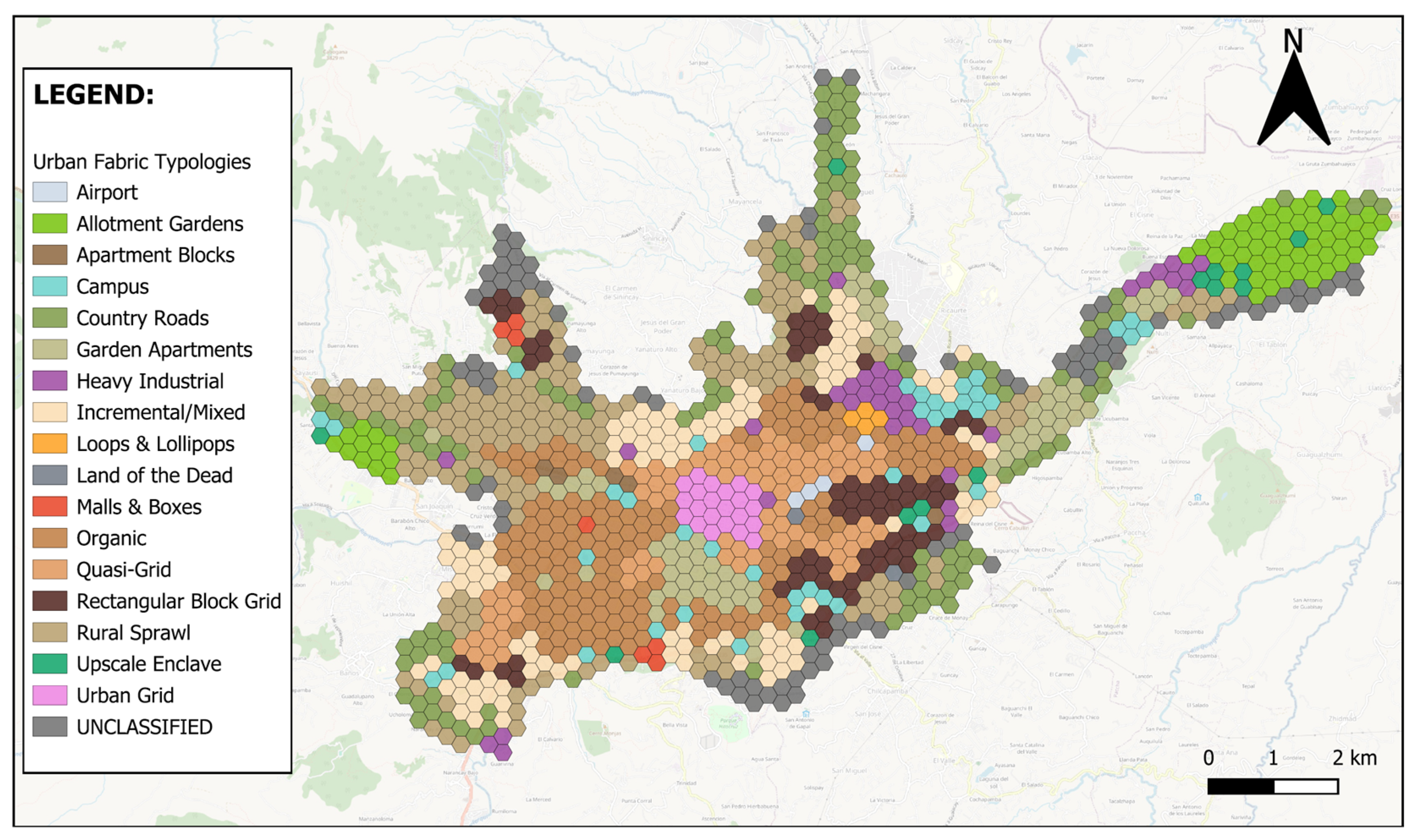
Figure 2. Correlation plot among USIs.

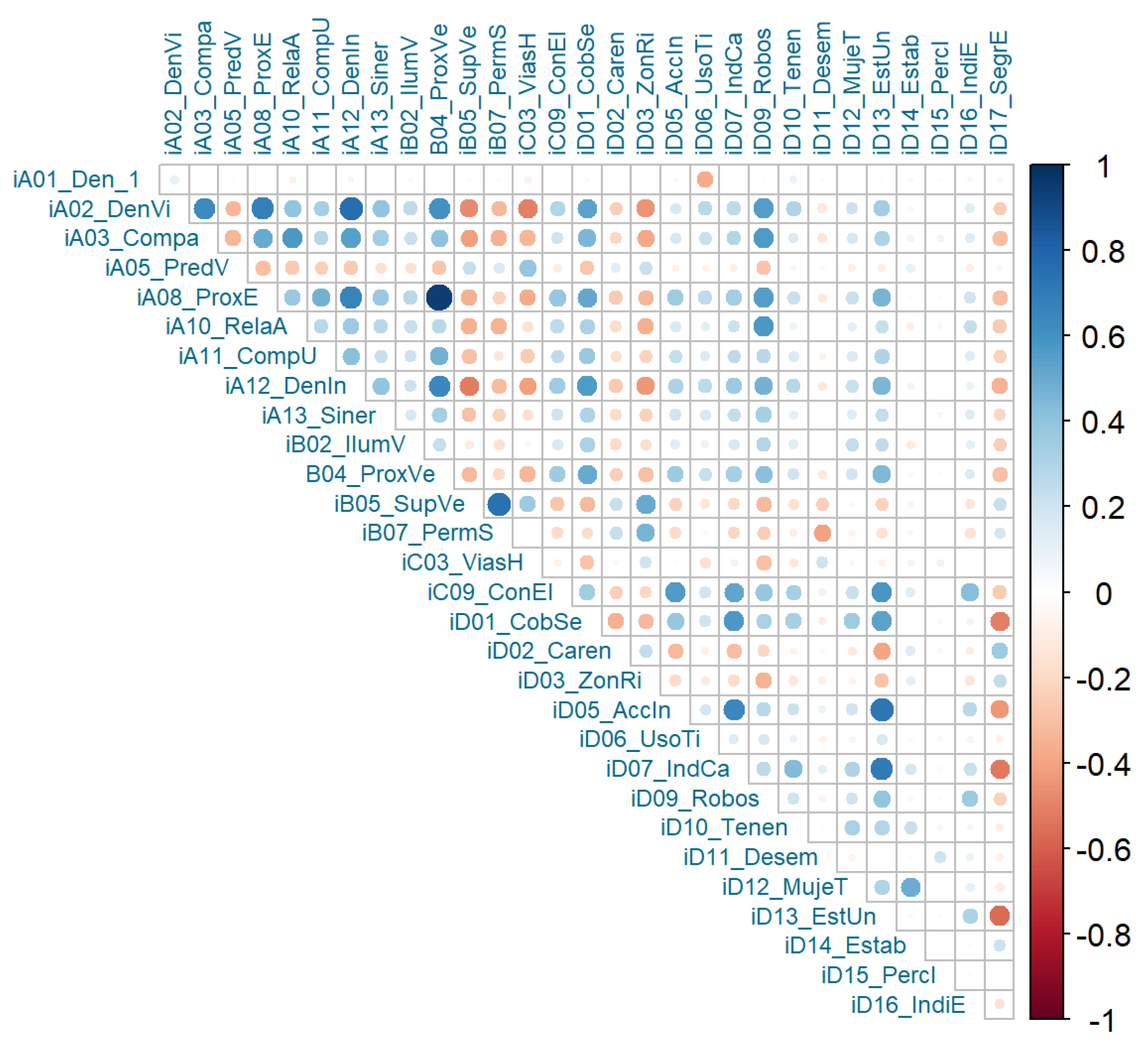
Figure 3. Scree plot for the top 10 components in terms of variance explained.

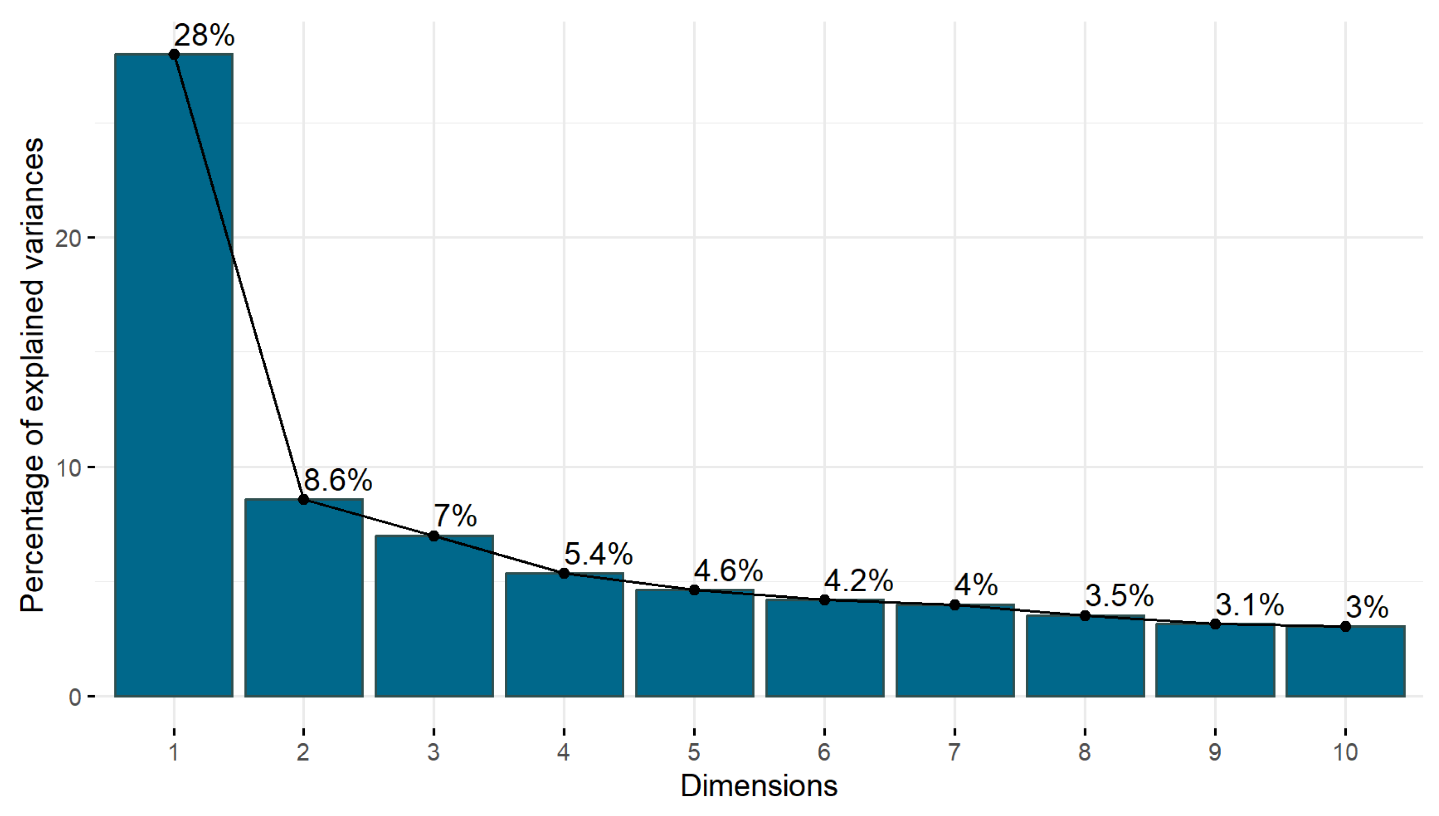
Figure 4. Boxplots of overall sustainability index by UFT, in ascending order.

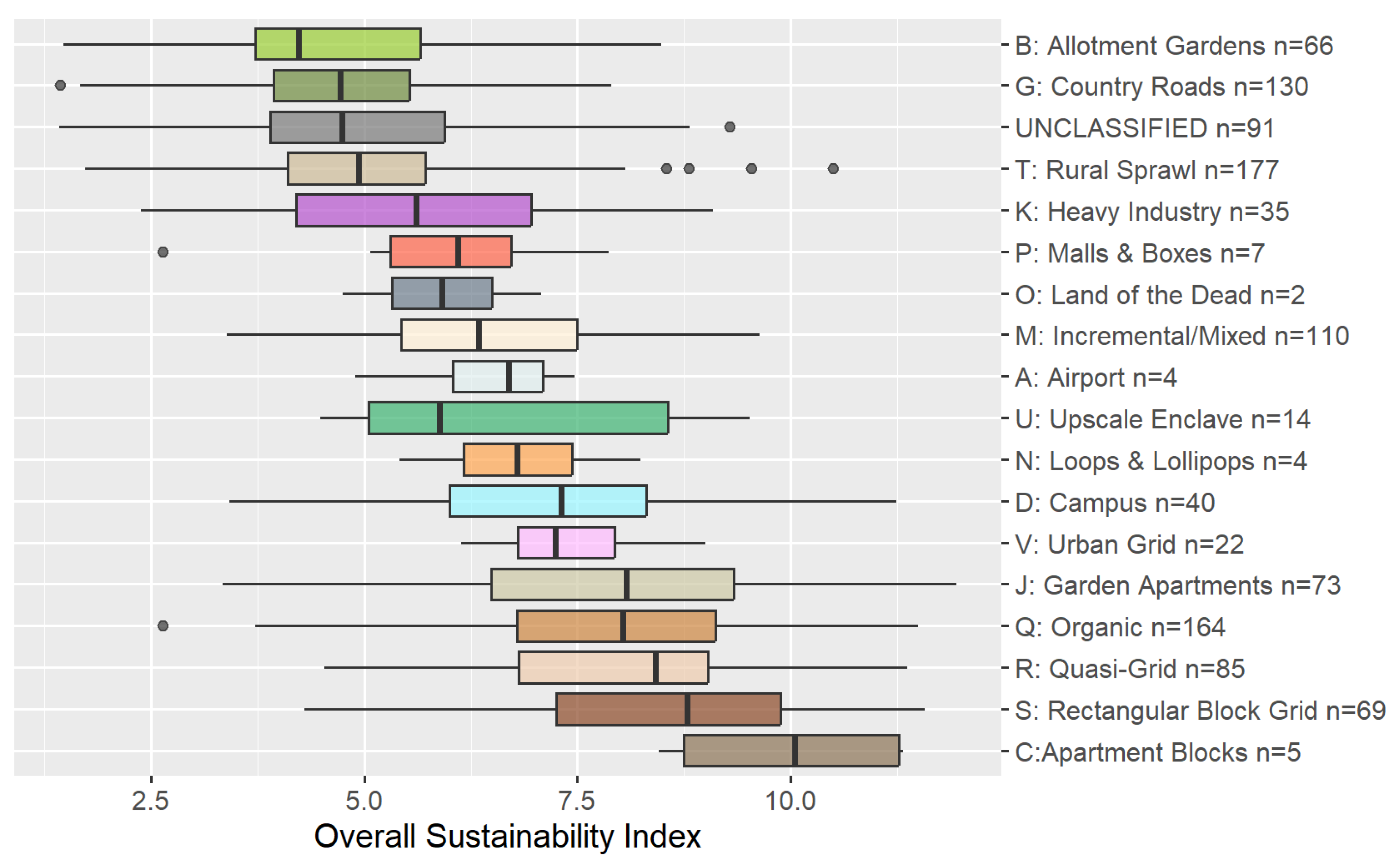
Figure 5. Choropleth of Cuenca´s grid overall sustainability index, labelled by UFT.

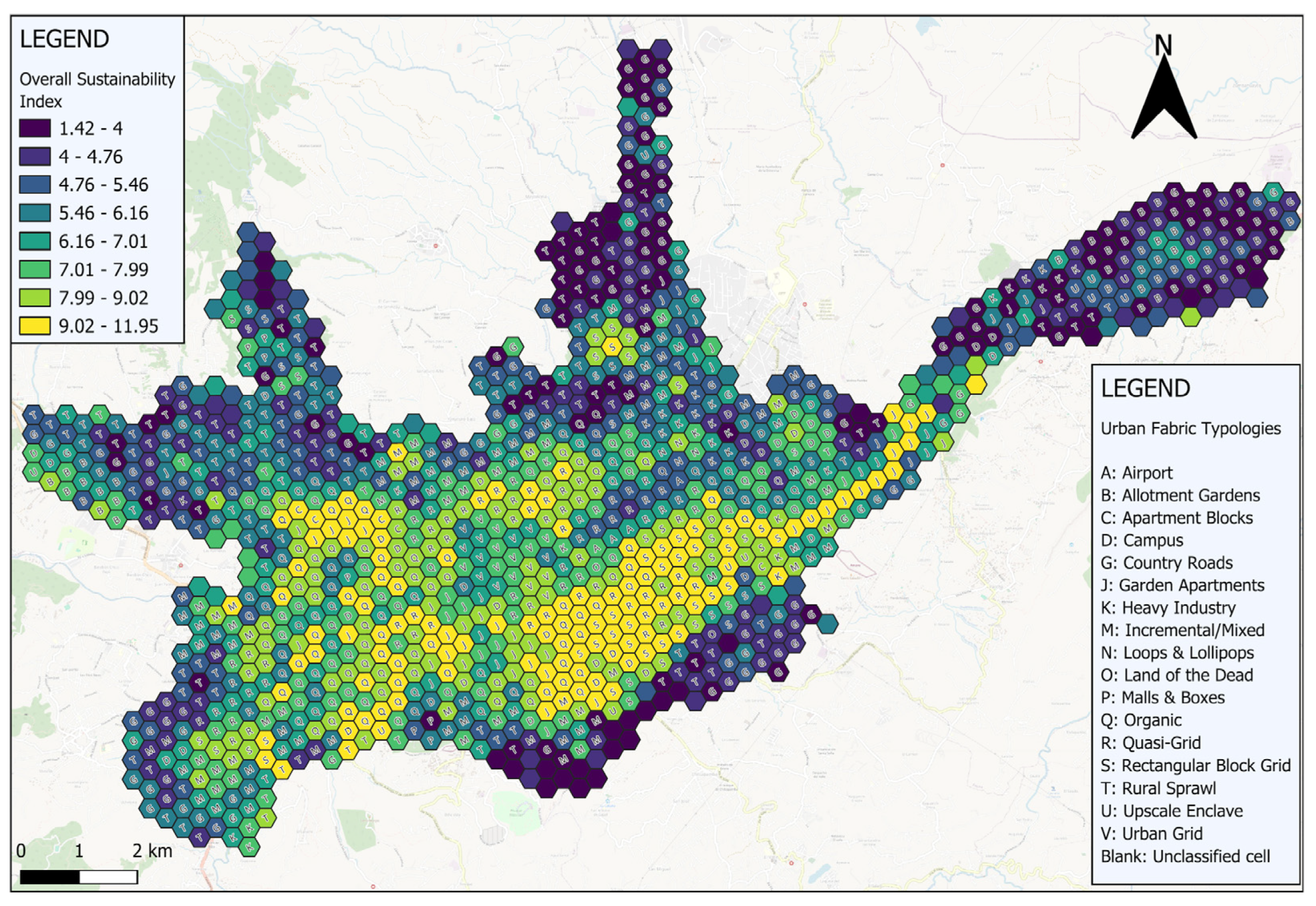
Figure 6. Choropleth of Cuenca´s hexagonal grid, characterised by the two highest and two lowest sustainability index ranges and labelled by UFT.

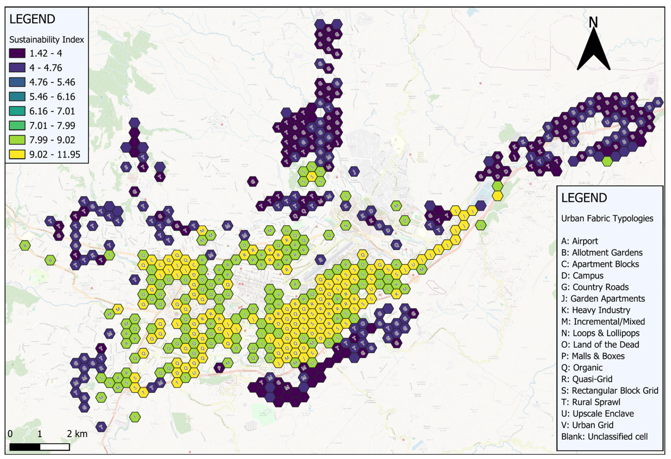
Figure 7. Choropleth of Cuenca´s hexagonal grid, characterised by UFT and the four mid-ranges of the sustainability index.

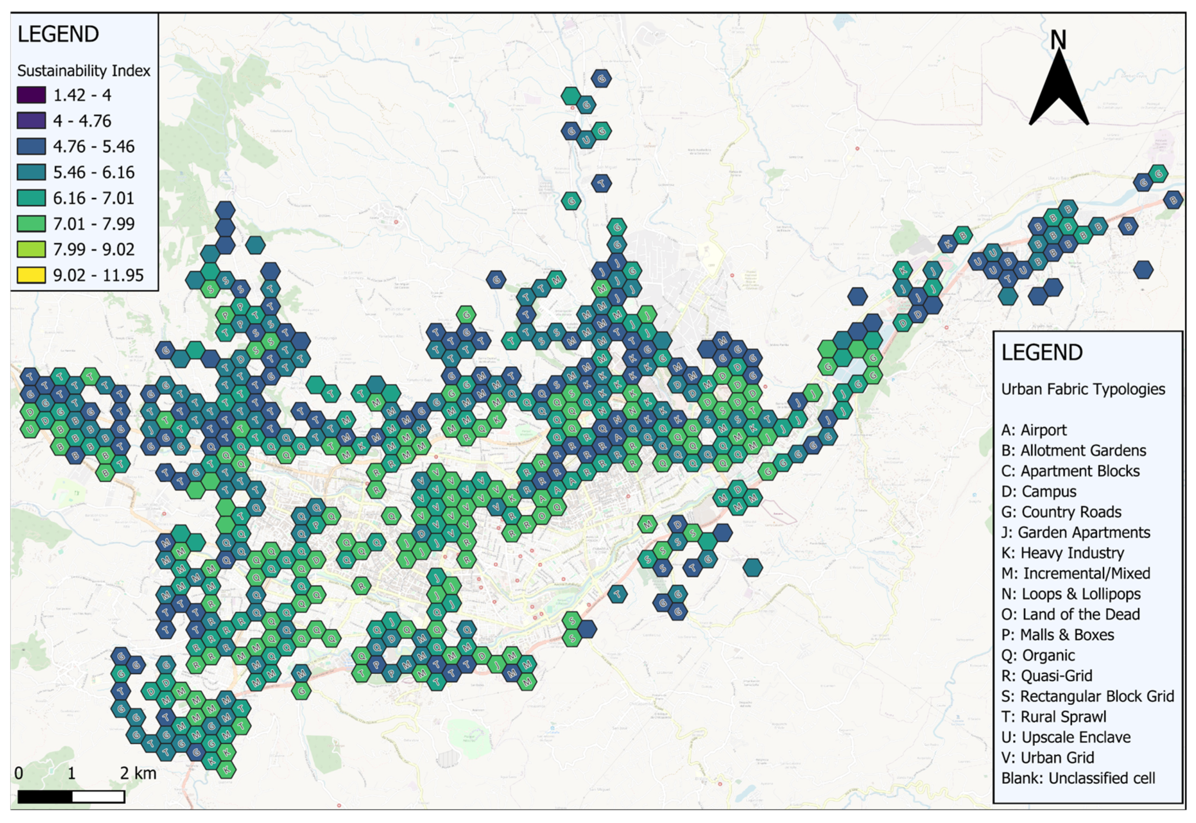
Figure 8. Spatial patterns for each high-level sustainability dimension.

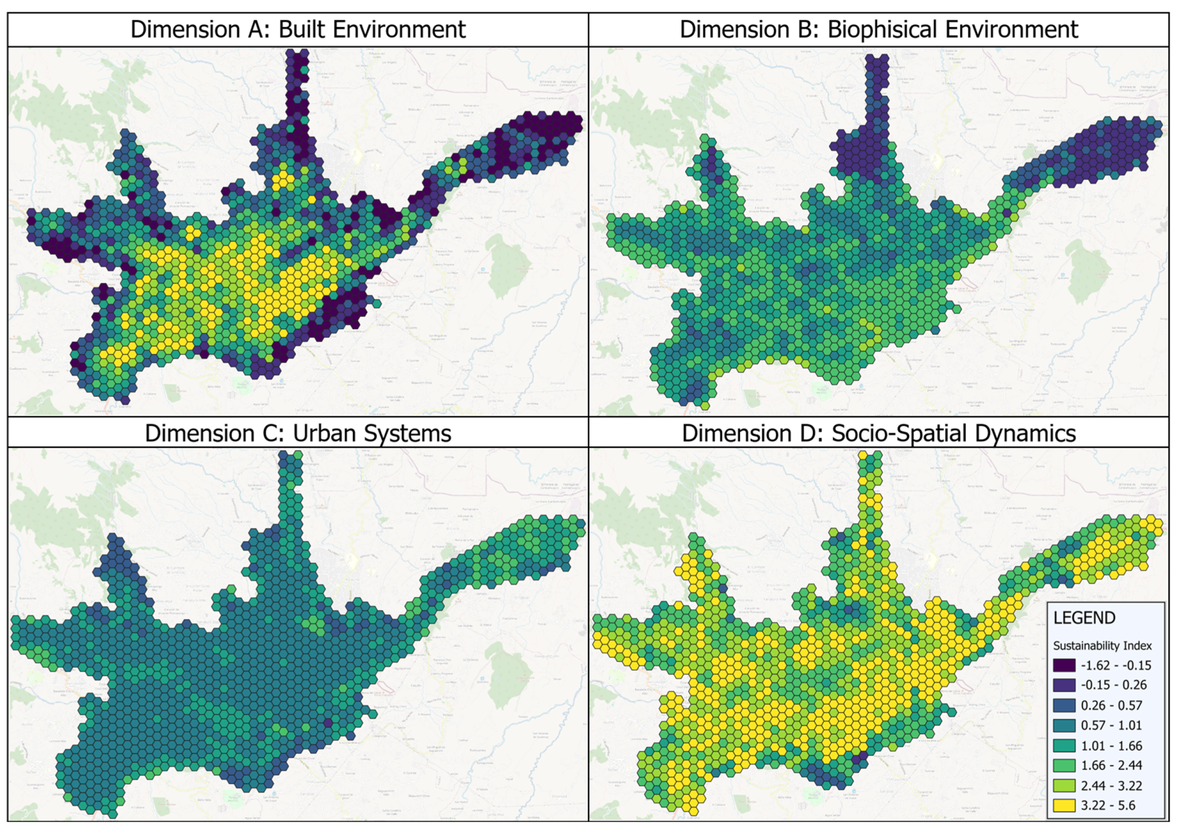
Table 1. Characteristics of the study area.

Study Area: Cuenca (as of 2022, the latest national census)1
Area	7248.23 ha
Inhabitants	361524
Households	115477
Population Density	49.87 inh/ha
Household Density	15.93 households/ha

Table 2. Sustainability indicators for the city of Cuenca.

No.	Name	Description
Dimension A: Built Environment
A01	Net population density	Number of houses per hectare. It evidences the consumption of residential land.
A02	Net housingdensity	Number of Inhabitants per hectare.
A03	Absolutecompactness	Building intensity equivalent to building volume on a given surface.
A05	Empty lot areas	Percentage of unused land or buildings on the block.
A07	Proximity to basic urban facilities	Percentage of households with simultaneous access within 500m to all types of basic urban facilities.
A08	Proximity to open public space	The percentage of households within a 5-minute walk of at least one type of open public space (park, plaza, sports field, riverbank, open market).
A09	Accessibility to purchasing basic daily supplies.	Percentage of households with simultaneous coverage within a 300m radius of different basic supplies necessary for daily life.
A10	Relation between activity andresidence	Urban variety and equilibrium are measured by the proportion of non-residential economic activities (commerce, services, offices) and the number of households. This indicator reflects a territory’s capacity to be self-contained in terms of mobility.
A11	Urban complexity	Diversity and frequency of land uses. It relies on Shannon´s formula of entropy [24] to evidence the mixture of activities.
A12	Pedestriancrossings density	Pedestrian connectivity of a territory, as the proportion of street pedestrian crossings to the whole study area.
A13	Synergy	Degree to which the internal structure of an observational unit relates to a higher scale at the system level, according to spatial syntax theory.
Dimension B: Biophysical environment
B01	Air quality index	Amount of population not exposed to emission levels beyond the maximum permitted by Ecuadorian normative. Contaminants considered simultaneously (NO₂, CO, SO₂, O₃, MP_2.5, and MP₁₀).
B02	Nocturnalillumination of public streets	Proportion of the number of illumination devices to the lineal kilometres of public streets. Measures the perception of safety associated with illumination.
B03	Acoustic comfort	Amount of population not exposed to noise levels beyond the maximum permitted by Ecuadorian normative. Max noise levels are 70dB at day and 65dB at night.
B04	Proximity to green spaces	Closeness of the population to the nearest green space.
B05	Green area perinhabitant	Ratio of public green space and the number of inhabitants.
B07	Soil permeability	Area of permeable soil with respect to total area. It relates to loss of permeability caused by urban expansion, in terms of buildings and pavement.
Dimension 3: Urban Systems
C03	Public roads per inhabitant	Ratio of public road lanes (lineal metres) and population.
C04	Proximity to alternative transport networks	Percentage of the population with simultaneous access to at least three alternative transport networks within 300m (bus, public bike share, bike paths, pedestrian paths; 500m for tram).
C09	Electricityconsumption of the household	Ratio of electricity consumption of the household by the number of residents in the household.
C13	Wastewatercoverage	Percentage of households connected to the public wastewater system.
Dimension D: Socio-spatial integration
D01	Households fully covered by basic services	Percentage of households with simultaneous access to drinkable water, electricity, wastewater and solid waste disposal.
D02	Households with critical construction defects	Percentage of households with critical construction defects (that can endanger residents).
D03	Dwellings located at risk zones	Percentage of households located at risk zones (landslide, flooding, topographically compromised, geologically compromised, agricultural zones, forestry zones, natural protection zones).
D05	Internet access	Percentage of households that can connect to internet services by computer or mobile.
D06	Use of time	Average time spent on personal activities within a working week (Mon-Fri), for the population aged 12 years and older.
D07	Life conditionsindex	Level of scarcity or abundance of the following household variables: a) physical characteristics; b) basic services; c) education of residents aged 6 years and older ; d) access to health insurance.
D08	Closeness andaccess to food	Spatial distribution of the city in terms of food purchasing locations (understood as: within 10 minutes from a public market).
D09	Thefts per year	Ratio of thefts to people, households, institutions, retail and vehicles in the study area, to the total thefts in the city.
D10	Housing security	Percentage of households with secured access to a dwelling (owned or rented).
D11	Unemployment rate	Percentage of the economically active population (aged 15 and older) that is unemployed.
D12	Women at paid workforce	Percentage of paid women in the workforce with respect to total employment (excluding agriculture).
D13	Economicallyactive population with a university degree	Percentage of the economically active population (aged 15 and older) with a completed university degree.
D14	Stability ofcommunity	Percentage of the population living in the same place (parish) for 5 or more years.
D15	Unsafetyperception	Percentage of citizens that feel unsafe in their neighbourhoods.
D16	Population ageing index	Quantitative ratio of older-adult population (aged 65 and more) to infant-young population (aged 0 to 15).
D17	Spatialsegregation	Level of exclusion, cohesion or segregation of the population with greater shortcomings (who fall within the first quartile of the Life Quality Index).

Table 3. Results from individual one-way ANOVA tests.

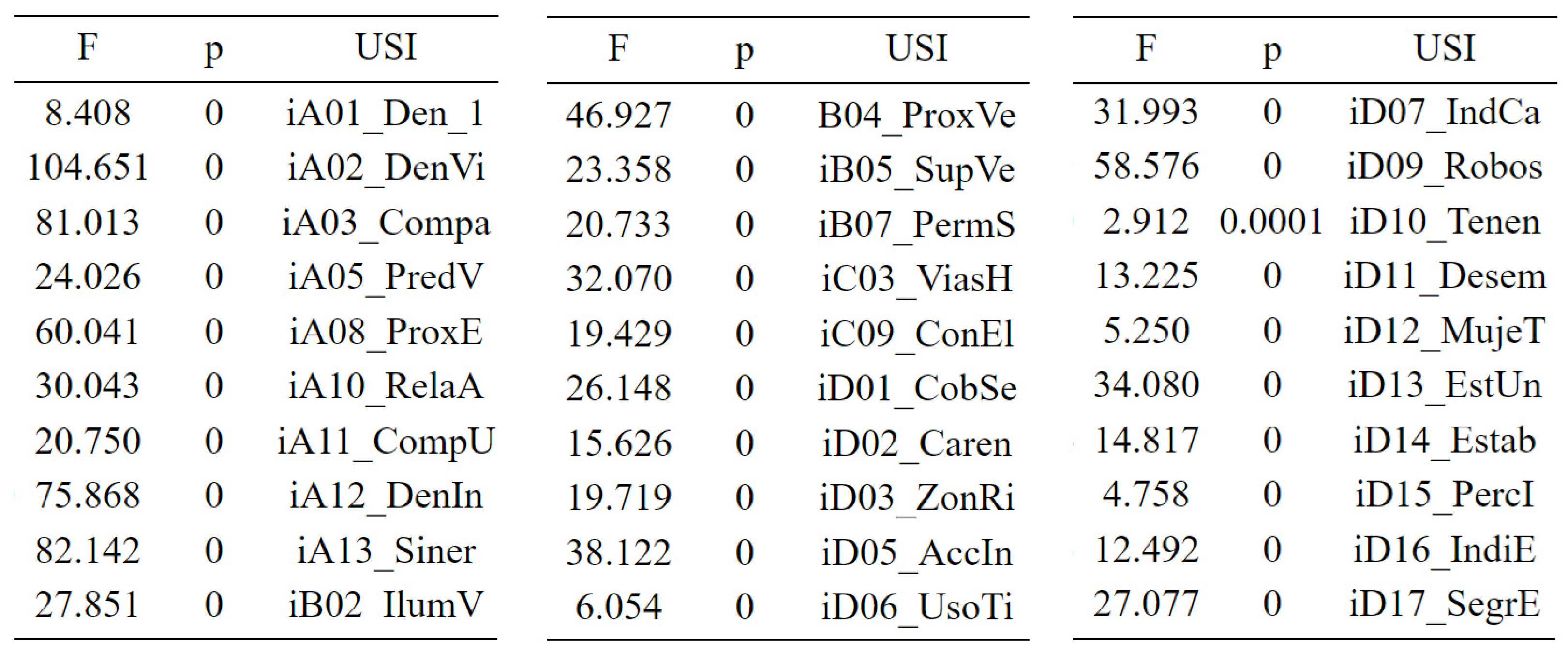
Table 4. Results from Tukey’s Honest Significant Differences test.

Disclaimer/Publisher’s Note: The statements, opinions and data contained in all publications are solely those of the individual author(s) and contributor(s) and not of MDPI and/or the editor(s). MDPI and/or the editor(s) disclaim responsibility for any injury to people or property resulting from any ideas, methods, instructions or products referred to in the content.

© 2024 by the authors. Licensee MDPI, Basel, Switzerland. This article is an open access article distributed under the terms and conditions of the Creative Commons Attribution (CC BY) license (http://creativecommons.org/licenses/by/4.0/).

Copyright: This open access article is published under a Creative Commons CC BY 4.0 license, which permit the free download, distribution, and reuse, provided that the author and preprint are cited in any reuse.

Alerts

MDPI Initiatives

Important Links

Choose an area of interest and we will send you notifications of new preprints at your preferred frequency.

Disclaimer