Submitted:
07 August 2024
Posted:
09 August 2024
You are already at the latest version
Abstract
In this paper, based on the cumulated damage generated by the cyclical application of the testing vibration profile, a methodology to determine the reliability index of the analyzed component is given. In the analysis, the testing time, component geometry, applied weight, and material resonant frequency are all of them considered by using a dynamic, and amplitude factor. Then, from the generated vibration response data of the analysis, the corresponding bending stress is determined for each one of the rows of the testing profile. And by the cyclical application of the whole testing profile, the corresponding damage is cumulated to each profile cycle until the cumulated damage is D=1. Finally, the reliability that each one of the cumulated blocks (cyclical profile application) is determined by considering, the random vibration is a stress variable. Thus, we use the cumulative damage model with the inverse power law stress/life relationship to determine the two parameter Weibull distribution used to estimate the reliability index of each cumulated block. As a numerical application, we analyze a cantilever aluminum beam Al 6061-T6.
Keywords:
random vibration
; Weibull reliability
; mechanical design
; cumulative damage model
; static and modal analysis
1. Introduction
Nowadays, most of the mechanical elements are subjected to vibration generated by cyclical loads. These cyclical loads cumulate fatigue damage to the element [1]. Therefore, to avoid failures generated by random vibration, in practice the dynamic element performance is evaluated trough a vibration test. Generally, the test is focused on determining the material strength, and the component’s reliability [2,3]. However, when the focus consists of determining if an element will perform its function without failure, we use a demonstration test. This test is based on a designed standard vibration profile, as they are those given in norm ISO16750-3 [4]. Thus, the vibration test is carryout by testing without failure a set on parts, for a constant test time , and by applying the acceleration energy (Grms) that corresponds to the used testing profile [5]. However, because it is a zero-failure approach, then once we complete the test, the element reliability remains unknown.
Therefore, with the focus of determining the element’s reliability, a functional test is performed by applying cyclically the whole test profile. From the application data of it test, the cumulated damage in each block (whole test profile cycle) is determined mainly by using the linear Miner rule [6], or the nonlinear curve damage model [7,8]. In both accumulated damage models, we considering the elements fails when the cumulated damage in the th-block is . Here, it is important to mention that because the Miner rule is linear, and it considers the applied vibration load to be constant, then between both approaches, we recommend using the second one. Moreover, observe that although in both approaches , the real reliability element remains unknown. Therefore, to consider the effect that geometry, weight, and resonance have on the accumulated damage, into the initial test profile, we incorporate in it the response acceleration that contains these effects.
In the application of an Al 6061-T6 aluminum cantilever beam we found the more significant resonance frequency was with an amplification factor of . From the analysis the generated damage was accumulated using the nonlinear curve model (eq.13). And the applied cycles were determined based on the Rainflow algorithm of the Matlab Vibrationdata library. In this case, the damage reaches the critical value of , after seven damage blocks. Finally, based on these damage blocks and addressed bending stress, by applying the cumulative damage model (eq.16) with the inverse power law model as the life/stress relationship, the shape and scale parameters of the Weibull distribution were estimated and used to determine the reliability index that corresponds to each one of the seven damage blocks (see Section 4.2). The generalities of the performed vibration analysis are as follows.
2. Generalities of Vibration Analysis
Damage vibration analysis is performed to elements that are subjected to fatigue. Its the accumulation is a complex process because it presents a nonlinear behavior. Among the models used to cumulate it, we have the three-band technique [9], the Miner’s rule and the nonlinear curve damage model. They generalities are.
2.1. Three-Band Technique Generalities
The Steinberg three-band technique is a simplified method for analyzing fatigue failure due to random vibrations by using Miner’s rule approach. Unfortunately, it let us a quick estimation of damage, as [10] mention it is not accurate. The method is based on the three bands of the normal distribution [9].
- values occur 68.3% of the time.
- values occur 27.1% of the time.
- values occur 4.33% of the time.
Where is the standard deviation of the normal distribution. Therefore, to perform the fatigue damage analysis we determine the expected number of applied cycles of each one of the three bands, and their corresponding stress. Then these stresses values are used in the S-N curve to determine the corresponding cycles to failure [9,11,12] that we use in the Miner rule approach.
2.2. Miner’s Linear Rule Model
Miner (1945) [13] based on the work of Langer, applied the linear damage rule to axial stress-strain fatigue data of aircraft raw material (see Figure 1). He found an agreement between the predictions of the linear damage rule and his experimental results [14]. The principle of accumulated damage using Miner's rule is performed based on the assumption that fatigue strength is determined by applying different levels of stress. Where each stress level contributes to a certain amount of damage. Thus, Miner’s rule is used to predict the total life of a component subjected to a sequence of load levels, and it is given by eq.(1);
where is the number of cycles of a specific stress level, is the number of cycles to failure for this stress level and is the damage that the material has suffered during the application of the applied load. Thus, , means that the component or part does not fail. In general, for several stress levels the cumulate damage is as in eq.(2), and as in Figure 1;
Therefore, the component failure is predicted when . From eq.(1), it is observed that the Palmgren-Miner rule is a simplistic model. It has no conclusive meaning because it does not allow us to evaluate probabilistically the selected design, which is fundamental in vibration fatigue analysis. Currently the Palmgren-Miner (1945) [13], and Palmgren (1924) approaches are still being used in most standards related to fatigue design to incorporate probability to the analysis. Moreover, from an engineering perspective, it is reasonable to consider damage as the probability of failure, derived from the field of the S-N curve, which agrees with the conventional concept of ultimate limit state (strength) [15]. However, to avoid the Miner’s rule disadvantages the nonlinear curve model was formulated.
2.3. Nonlinear Damage Curve Model
The double lineal damage model by Manson and Halford rule is used to determine the damage of an element subject to vibration [16]. This model considers the interactions of the applied load and the nature nonlinear behavior of the vibration. It considers equal damage for the two load levels based on the theory of elasticity and material properties [16], the equivalent damage radius cycle is represented by
Consequently, the damage curve model is given by the power law equation.
where the exponent 0.4 represents the cause-effect relationship of the deformation of the material with the applied cycles. To consider the effect of the PSD (power spectral density) loads, the exponent of the previous model was modified by [7,17] to be the model a function of the loads. It was formulated by substituting the exponent 0,4 by . Thus, the developed model is a nonlinear continuous damage function that incorporates the vibration-induced bending stress as follows
In this paper we used to accumulate the damage generate by vibration analysis by using the nonlinear model defined in eq.5. Where the cycles to failure is determined by the Basquin equation
The numerical application is as follows.
3. Application Case
In the numerical case, we used the analyzed cantilever beam published in [18]. Its has the following proprieties, aluminum Al 6061-T6, elasticity modulus , Poisson’s ratio =0,3, yield strength , ultimate tensile strength , fatigue strength density , and length by wide by high, as it is shown in Figure 2. An overall damping ratio of percent is considered in the analysis. The beam supports a weight of mounted on the tip of the beam, and its movement is restricted to only vertical direction. The mechanical element must be capable of operating in a white-noise random vibration environment with an input PSD level of , and a frequency range of for a period of . In [18], the vibration analysis was performed by the lineal damage by Miner’s rule as follows.
3.1. Three Bands Miner’s Rule Analysis
The lineal three bands Miner’s rule analysis is performed with the objective of determining the cumulated damage that will cause the failure of the element under random vibration. Here we present only the generalities of the study case, for details see [18]. In their analysis, they found the material natural frequency is , with bending stress of . Stress results as shown in Table 1.
The applied cycles were determined by considering a test time of four hours. Thus, the applied cycles are,
In the analysis was considered as the base cycle. Therefore, the cycles to failure that corresponds to each one of the three Gaussian bands are determined as,
where is the material fatigue coefficient of the aluminum Al 6061-T6. Numerically, they are.
Therefore, by using the Miner’s Rule defined in eq.(2) with the addressed and values, they found that the cumulative damage was , implying that the remaining useful life is . for details see [18].
Unfortunately, based on this lineal analysis, we cannot address the reliability of the analyzed component, mainly because the spread of the vibration data and its no lineal behaving were not considered. Therefore, we use the non-linear method to cumulate the damage and to considered randomness of the vibration data.
3.2. No Lineal Analysis
To take randomness into account and to be able to determine reliability, the non-linear method is considered. We use in the study case, a range frequency of with an acceleration of . The test profile is given in Table 2.
However, because this profile does not contain the testing time effect, then we simulate it in Matlab as follows
3.2.1. Incorporation of Time to the Test Profile
To consider the test time of 4 hrs. (7200 sec) the Matlab Vibrationdata library was used. From output the response acceleration plot is shown in Figure 3, and the corresponding response acceleration data is given in Table 3.
Here notice by comparing Table 2 with Table 3, the acceleration was increasing because the testing time has over the vibration damage. However, although now we are considering the time effect in the analysis, because the geometry, weight, and resonance effect are not considering yet, we perform the corresponding static and modal analysis as follows.
3.2.2. Static and Modal Analysis
To incorporate geometry, weight, and significant resonance into the analysis the corresponding angular natural frequency in , is determinated as.
where is the modulus of elasticity in , is the inertia moment in , is the defective mass of the load in , and is the length of the component in . Numerically, is estimated as
Thus, based on the corresponding natural frequency is,
3.2.3. Bending Stress Analysis
The bending stresses used to calculate the cycles to failure, based on the response acceleration from Table 3, and the dynamic factor given in eq.(10) are presented in Table 4. It is determined as
Based on the bending stress in Table 4 and Basquin’s formula defined in eq.6, by using the bending stress is given by
The corresponding cycles to failure are presented in Table 5. The used fatigue coefficients in eq.12 are and .
On the other hand, the applied cycles corresponding to each damage block are determined using the Rainflow algorithm (ASTM E 1049-85) of Matlab. The applied cycles are given in Table 6.
3.2.4. Determination of Accumulation Damage
The accumulation of the vibration damage is performed by using the nonlinear curve model [17] as.
The accumulated damage until is given in Table 7.
From Table 7, we notice the damage (fatigue failure) is reached in block 7. The corresponding nonlinear cumulated damage behavior is shown in Figure 4.
At this point, it is important to mention that although the cumulative damage already contains the effect of test time, geometry, weight, and resonance, still it is not possible to determine neither the reliability of the element nor the reliability that each of the damage blocks present. Thus, in this paper to determine those reliabilities we use the cumulative damage model for variant stress as shown in the following section.
4. Cumulative Damage Model
In vibration analysis the main problem is that, since the vibration is random in nature its analysis must be performed considering it as a variant stress. Because vibration is random in nature, it difficult to determine the number of cycles that correspond to each one of the significant frequencies of the vibration spectrum (profile). This implies that when we are using these cycles in the Miner’s rule, the corresponding accumulated damage is not representative of the damage generated by the vibration [21].
In the other hand, to make the estimated cycles representative of the vibration, in this paper, to the initial vibration profile given in [18], we incorporate to it the effect that geometry, weight, and resonance have on the accumulated damage. The effect of geometry, weight, and resonance is incorporated by performing the static and modal analysis (see Section 3.2.3). As a result, the estimated stress for each one of the row’s profiles, by using a dynamic factor (see Section 3.2.4) are representative of the accumulated vibration damage. Thus, due to these stresses are used in the S-N curve for determining the cycles to failure , then these are also representative of the accumulated damage. Here it is important to mention that, although up to this point, the are now representative of the vibration, they should not be used in Miner’s rule to accumulate the generated damage because the accumulated damage presents a nonlinear behavior. Therefore, we use the accumulated damage model to estimate the reliability of the analyzed element.
4.1. Cumulative Damage Model Formulation
The cumulative damage model can be defined as the amount of damage , at a given stress level [14]. And it is widely used to determine the reliability of an element when it is subject to time-varying stress. Among the most common damage models, we have the step stress method where the element is subjected to different stress levels [22,23]. And to consider the randomness of the analyzed phenomenon, a probability distribution is used. In our case, we use the two parameter Weibull distribution. The Weibull reliability function for the cumulative damage model is given by [24,25],
where is the block number (row) of the table of the cumulated damage, and the Weibull scale parameter is given by,
where and are the parameters to be estimated. Therefore, the Weibull function/cumulative damage model is,
Here it is very important to notice that from eq.16 the Weibull/cumulative damage model is efficient for modeling vibration because the bending vibration stress that we use as the variable , is based on the acceleration response (see Table 3 and Figure 3) which was determined by simulating in random way the vibration profile. Thus, once the model parameters are determined, we can estimate the reliability of the element subjected to vibration as follows.
4.2. Weibull Cumulative Damage Reliability Indices
To determine the reliability of the product using the cumulative damage model define in eq.16, we use as an input the vibration response given in Table 8, which contains the estimated vibration stress (see Table 4), and its corresponding cyclical profile shown in Figure 5.
The parameters estimation ( and of eq.16 is performed by maximum likelihood estimator. Here we use the Alta software routine. The estimated parameters are given in Figure 6.
Therefore, by using , and the vibration stress that corresponds to the first row of Table 8 in eq.15, the Weibull scale parameter is . Consequently, the Weibull shape parameter given in Figure 6, and the addressed values are the Weibull family used to determine the corresponding reliability indices of the analyzed mechanical element. The reliability indices that correspond to each one of the seven blocks from Table 7 by using the Weibull parameters in eq.14 are given in Table 9.
From the first row of Table 9, notice that the reliability of the product after the first vibration cycle is , and it decreases to after the seven blocks. Additionally, from Table 9, also observe that although there seems to be a direct relationship between the cumulated damage and the indices. Further research is needed to identify a functional relationship between them.
5. Conclusions
1. The proposed methodology let us determine the Weibull family that represents the vibration analysis and the reliability index for each one of the cumulated damage blocks. Notice these reliability indices can be used to determine the remanent life to each block.
2. Through the proposed method, by using the cumulative damage model and the Weibull distribution as shown in Section 4, for any testing profile that contains the corresponding vibration bending stress (see Table 8), and by taking the number of blocks of the cumulative damage process as the corresponding lifetimes, the reliability of the element (first row from Table 9) as well as the reliability of each block can be always determined.
3. The cumulative damage presented in Table 7 is considered representative of the vibration environment, because it was accumulated using the nonlinear curve model given in eq.(13), and it was accumulated from the response profile that already contained the geometry effect, weight, and resonance frequency.
4. The incorporation of the geometry effect, weight, and resonance into the vibration analysis, makes the estimated vibration stresses to be representative of the cumulative damage generated by vibration.
5. Although in our case the critical damage occurred in the seventh block, in practice can be reached in any blocks. However, remember that in the proposed Weibull analysis the number of blocks for which must be used as the failure time in the Weibull analysis as shown in Figure 6.
Author Contributions
Conceptualization, M.M.H.-R., M.R.P.-M. and J.M.B.-C.; methodology, M.M.H.-R., M.R.P.-M. and O.M.-Q.; formal analysis, M.M.H.-R., M.R.P.-M. and J.M.B.-C.; writing—original draft preparation, M.M.H.-R. and M.R.P.-M.; writing—review and editing, M.M.H.-R., M.R.P.-M. and O.M.-Q.; supervision, M.R.P.-M.; funding acquisition, M.M.H.-R.; All authors have read and agreed to the published version of the manuscript.
Funding
This research received no external funding.
Institutional Review Board Statement
Not applicable.
Informed Consent Statement
Not applicable.
Data Availability Statement
Not applicable.
Acknowledgments
We appreciate the support of Conahcyt and the Autonomous University of Ciudad Juárez (UACJ) provided in this research.
Conflicts of Interest
The authors declare no conflicts of interest.
References
- M. R. Piña-Monarrez, “Weibull analysis for normal/accelerated and fatigue random vibration test,” Qual Reliab Eng Int, vol. 35, no. 7, pp. 2408–2428, 2019. [CrossRef]
- L. J. Wang and Z. W. Wang, “FEM verification of accelerated vibration test method based on Grms - T curve,” Advances in Mechanical Engineering, vol. 14, no. 2, pp. 1–12, 2022. [CrossRef]
- V. Rouillard and M. J. Lamb, “Using the Weibull distribution to characterise road transport vibration levels,” Packaging Technology and Science, vol. 33, no. 7, pp. 255–266, 2020. [CrossRef]
- I. O. for Standardization, “INTERNATIONAL STANDARD Road vehicles — Environmental conditions and testing for electrical,” 2012.
- L. Edson, “The GMW3172 Users Guide,” 2008.
- K. Hectors and W. De Waele, “Cumulative damage and life prediction models for high-cycle fatigue of metals: A review,” Metals (Basel), vol. 11, no. 2, pp. 1–32, 2021. [CrossRef]
- J. M. Barraza-Contreras, M. R. Piña-Monarrez, A. Molina, and R. C. Torres-Villaseñor, “Random Vibration Fatigue Analysis Using a Nonlinear Cumulative Damage Model,” Applied Sciences (Switzerland), vol. 12, no. 9, 2022. [CrossRef]
- S. S. Manson and G. R. Halford, “Practical implementation of the double linear damage rule and damage curve approach for treating cumulative fatigue damage,” 1981.
- D. S. Steinberg, Vibration analysis for electronic equipment. John Wiley & Sons, 2000.
- A. Al-Yafawi, S. Patil, D. Yu, S. Park, and J. Pitarresu, “Random Vibartion Test for Electronic Assemblies Fatigue Life Estimation,” IEEE, 2010.
- S. Qin, Z. Li, X. Chen, and H. Shen, “Comparing and Modifying Estimation Methods of Fatigue Life for PCBA under Random Vibration Loading by Finite Element Analysis,” IEEE, 2015.
- M. Zheng, F. Shen, and P. Luo, “Vibration Fatigue Analysis of the Structure under Thermal Loading,” in Advanced Materials Research, 2014, pp. 559–564. [CrossRef]
- M. A. Miner, “Cumulative Damage in Fatigue,” J Appl Mech, vol. 12, no. 3, pp. A159–A164, Sep. 1945. [CrossRef]
- Y.-L. Lee, J. Pan, R. Hathaway, and M. Barker, Fatigue Testing and Analysis. 2005.
- E. Castillo and A. Fernández-Canteli, A Unified Statistical Methodology for Modeling Fatigue Damage. 2009.
- W. Weibull, “A Statistical theory of the strength of materials,” pp. 1–45, 1939.
- J. M. Barraza, “Metodología para la Acumulación del Daño por Fatiga Provocado por Vibración Aleatoria,” Universidad Autónoma de Ciudad Juárez, 2022.
- S. M. Kumar, “Analyzing Random Vibration Fatigue,” ANSYS Advantage, vol. II, no. 3, pp. 39–42, 2008, [Online]. Available: www.ansys.com.
- J. M. Barraza-Contreras, M. R. Piña-Monarrez, and R. C. Torres-Villaseñor, “Vibration Fatigue Life Reliability Cable Trough Assessment by Using Weibull Distribution,” Applied Sciences (Switzerland), vol. 13, no. 7, 2023. [CrossRef]
- J. M. Barraza-Contreras, M. R. Piña-Monarrez, and R. C. Torres-Villaseñor, “Reliability by Using Weibull Distribution Based on Vibration Fatigue Damage,” Applied Sciences (Switzerland), vol. 13, no. 18, Sep. 2023. [CrossRef]
- J. M. Barraza-Contreras, M. R. Piña-Monarrez, and A. Molina, “Fatigue-Life Prediction of Mechanical Element by Using the Weibull Distribution,” Applied Sciences 2020, Vol. 10, vol. 10, 2020. [CrossRef]
- ReliaSoft, “Two Methods for Analyzing Time-Varying Stress Data in ALTA,” 2016.
- ReliaSoft, “Topics A Look Under the Hood at the Cumulative Damage Model,” 2003.
- H. Bruel and K. Inc, “Accelerated Life Testing Data Analysis Reference,” 2004.
- J. M. Barraza-Contreras, M. R. Piña-Monarrez, M. M. Hernández-Ramos, O. Monclova-Quintana, and S. Ramos-Lozano, “Acceleration of Service Life Testing by Using Weibull Distribution on Fiber Optical Connectors,” Applied Sciences, vol. 14, no. 14, p. 6198, Jul. 2024. [CrossRef]
Figure 1.
Miner’s cumulative damage.
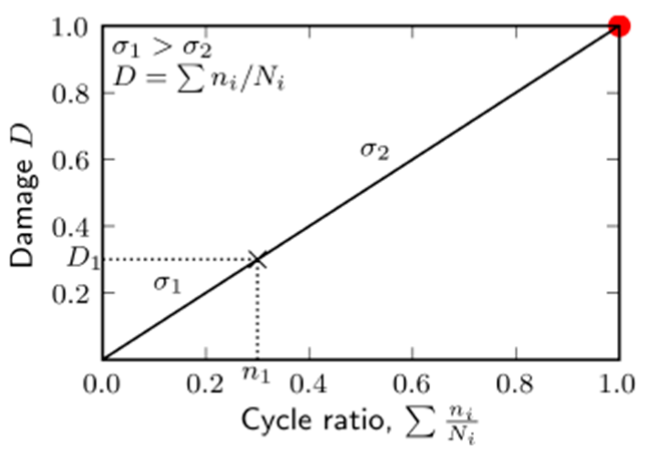
Figure 2.
Aluminum cantilever beam, [19].
Figure 2.
Aluminum cantilever beam, [19].

Figure 3.
Acceleration synthesis.
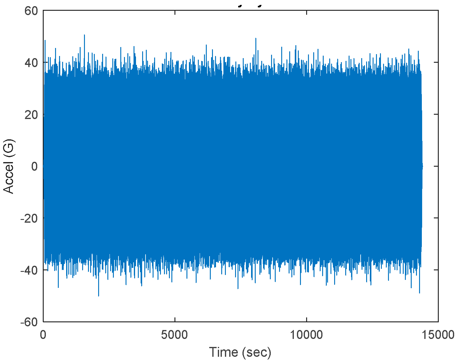
Figure 4.
Damage curve behavior.
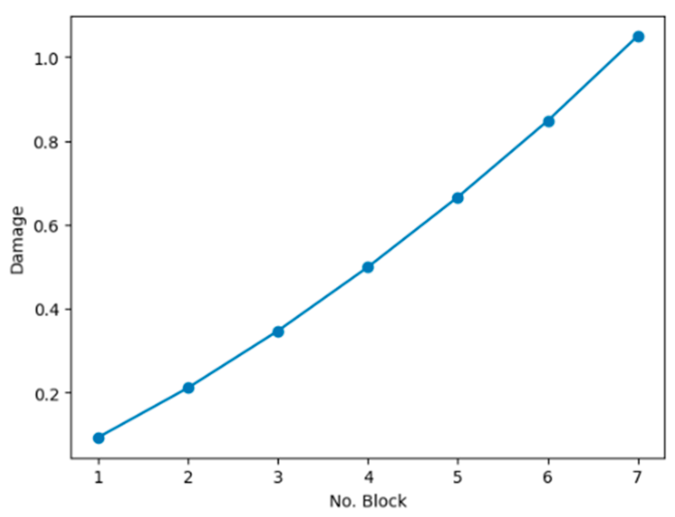
Figure 5.
Cyclical profile behavior.
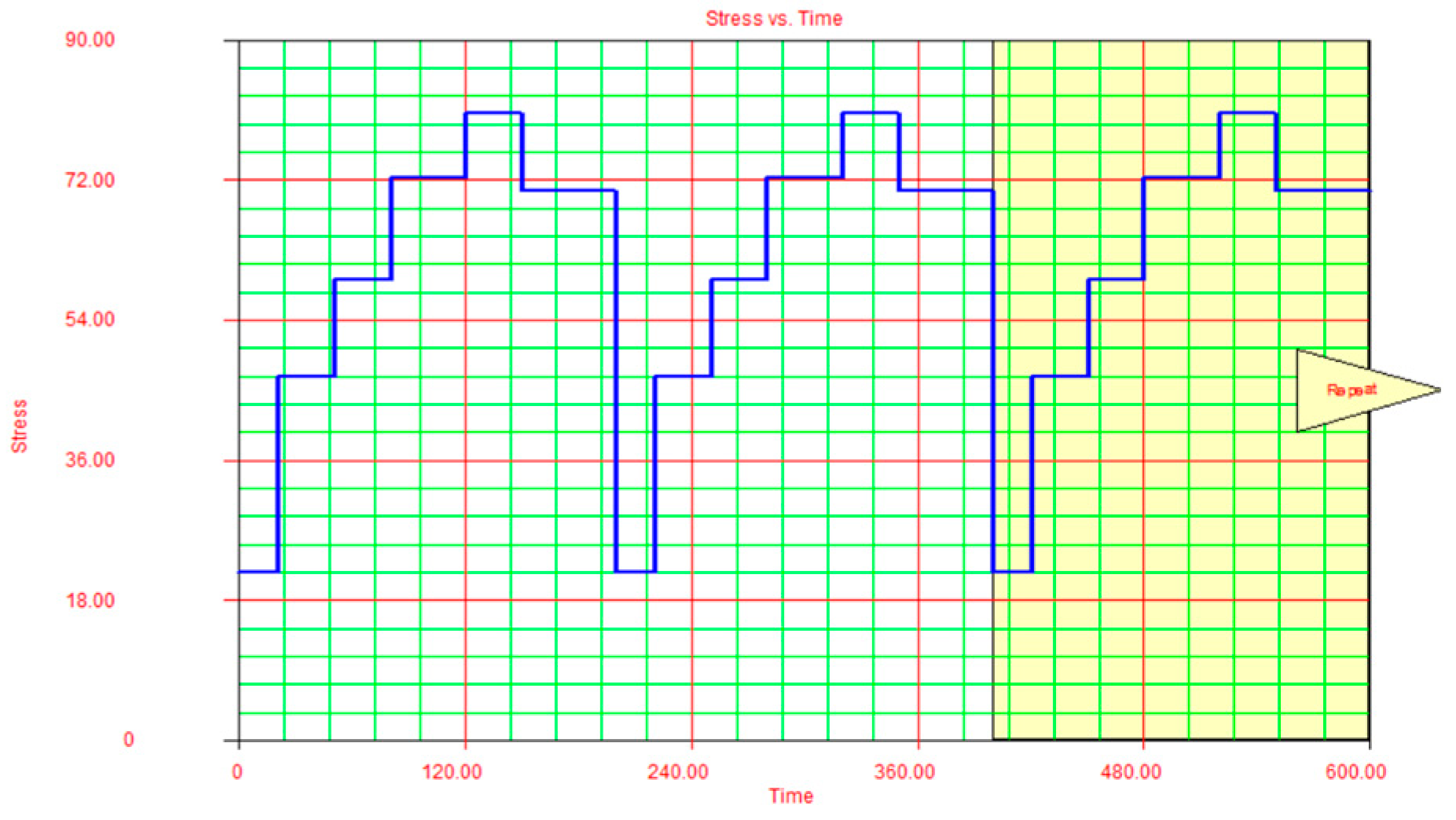
Figure 6.
Vibration profile.
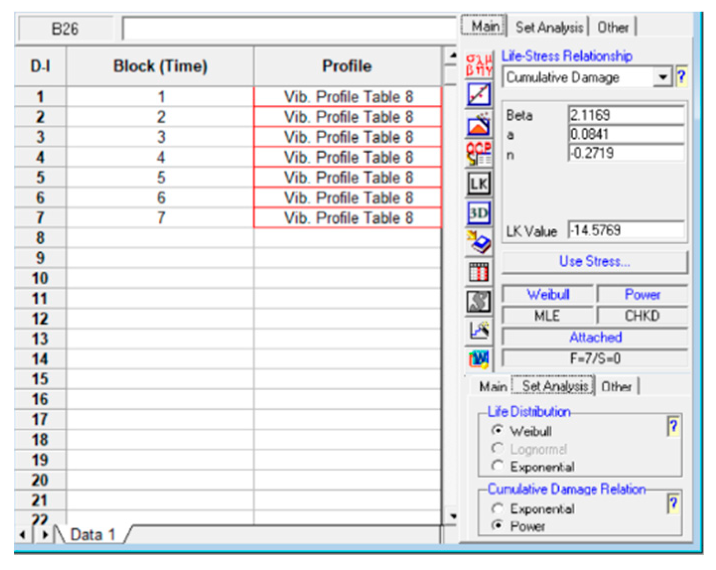

Table 1.
Maximum stresses [19].
Table 1.
Maximum stresses [19].
| Standard Deviation | Bending Stress | Percentage of Occurrence |
|---|---|---|
| stress | 1 ∗ 55.4 = 55.4 MPa | 68.3% |
| stress | 2 ∗ 55.4 = 110.8 MPa | 27.1% |
| stress | 3 ∗ 55.4 = 166.2 MPa | 4.33% |
Table 2.
Input profile.
| Frequency (HZ) |
Gravities (G) |
Acceleration [G^2/Hz] |
|---|---|---|
| 20 | 3.082 | 0.475 |
| 50 | 4.873 | 0.475 |
| 80 | 6.164 | 0.475 |
| 120 | 7.550 | 0.475 |
| 150 | 8.441 | 0.475 |
| 200 | 9.747 | 0.475 |
Table 3.
Response acceleration.
| Frequency (Hz) | Input acceleration (G) | Response acceleration (Ares in G) |
|---|---|---|
| 20 | 0.475 | 8.88 |
| 50 | 0.475 | 19.21 |
| 80 | 0.475 | 24.33 |
| 120 | 0.475 | 29.77 |
| 150 | 0.475 | 33.17 |
| 200 | 0.475 | 29.03 |
Table 4.
Vibration profile with bending stress.
| Frequency (Hz) |
Response Acceleration Ares (G) | (Mpa) |
(Mpa) |
|---|---|---|---|
| 20 | 8.88 | 2.42 | 21.5784 |
| 50 | 19.21 | 46.6803 | |
| 80 | 24.32 | 59.0976 | |
| 120 | 29.77 | 72.3411 | |
| 150 | 33.17 | 80.6031 | |
| 200 | 29.03 | 70.5429 |
Table 5.
Results of cycles to failure .
| Frequency (HZ) |
(Mpa) |
(Cycles to Failure) |
|---|---|---|
| 20 | 21.5784 | 1.40E+10 |
| 50 | 46.6803 | 1.02E+08 |
| 80 | 59.0976 | 2.28E+07 |
| 120 | 72.3411 | 6.28E+06 |
| 150 | 80.6031 | 3.15E+06 |
| 200 | 70.5429 | 7.37E+06 |
Table 6.
Applied cycles Rainflow.
| Frequency (Hz) | (applied cycles) |
|---|---|
| 20 | 110437 |
| 50 | 74883.5 |
| 80 | 114802 |
| 120 | 137055 |
| 150 | 249066 |
| 200 | 156561.5 |
Table 7.
Results of the accumulated damage calculation.
| 20 Hz | 50 Hz | 80 Hz | 120 Hz | 150 Hz | 200 Hz | ||||||
|---|---|---|---|---|---|---|---|---|---|---|---|
| Block No. | D1 | neq+n2 | D1+2 | neq+n3 | D1+2+3 | neq+n4 | D1+2+3+4 | neq+n5 | D1+2+3+4+5 | neq+n6 | D1+2+3+4+5+6 |
| 1 | 7.88E-06 | 9.84E+06 | 8.18E-06 | 2.07E+06 | 1.07E-05 | 1.46E+05 | 1.36E-03 | 2.53E+05 | 8.04E-02 | 2.99E+06 | 9.27E-02 |
| 2 | 9.27E-02 | 6.37E+07 | 9.32E-02 | 1.40E+07 | 9.70E-02 | 1.80E+06 | 1.11E-01 | 6.00E+05 | 1.91E-01 | 4.09E+06 | 2.11E-01 |
| 3 | 2.11E-01 | 7.51E+07 | 2.12E-01 | 1.66E+07 | 2.19E-01 | 2.78E+06 | 2.40E-01 | 1.00E+06 | 3.19E-01 | 4.94E+06 | 3.47E-01 |
| 4 | 3.47E-01 | 8.30E+07 | 3.49E-01 | 1.84E+07 | 3.59E-01 | 3.64E+06 | 3.84E-01 | 1.46E+06 | 4.63E-01 | 5.66E+06 | 4.99E-01 |
| 5 | 4.99E-01 | 8.92E+07 | 5.01E-01 | 1.98E+07 | 5.15E-01 | 4.44E+06 | 5.44E-01 | 1.96E+06 | 6.23E-01 | 6.32E+06 | 6.66E-01 |
| 6 | 6.66E-01 | 9.45E+07 | 6.69E-01 | 2.11E+07 | 6.87E-01 | 5.20E+06 | 7.19E-01 | 2.52E+06 | 7.99E-01 | 6.92E+06 | 8.48E-01 |
| 7 | 8.48E-01 | 9.92E+07 | 8.51E-01 | 2.21E+07 | 8.73E-01 | 5.95E+06 | 9.09E-01 | 3.11E+06 | 9.88E-01 | 7.49E+06 | 1.05E+00 |
Table 8.
Alta input test profile.
| Frequency (HZ) |
(Mpa) |
|---|---|
| 0 - 20 | 21.5784 |
| 20 - 50 | 46.6803 |
| 50 - 80 | 59.0976 |
| 80 - 120 | 72.3411 |
| 120 - 150 | 80.6031 |
| 150 - 200 | 70.5429 |
Table 9.
Reliability for each block.
| Cumulative Damage (from Table 7) | Reliability (eq.14) | |
|---|---|---|
| 1 | 0.09267947 | 0.9598 |
| 2 | 0.21120544 | 0.8368 |
| 3 | 0.34716136 | 0.6569 |
| 4 | 0.49903841 | 0.4618 |
| 5 | 0.66617094 | 0.2896 |
| 6 | 0.84823089 | 0.1616 |
| 7 | 1.04506581 | 0.0800 |
Disclaimer/Publisher’s Note: The statements, opinions and data contained in all publications are solely those of the individual author(s) and contributor(s) and not of MDPI and/or the editor(s). MDPI and/or the editor(s) disclaim responsibility for any injury to people or property resulting from any ideas, methods, instructions or products referred to in the content. |
© 2024 by the authors. Licensee MDPI, Basel, Switzerland. This article is an open access article distributed under the terms and conditions of the Creative Commons Attribution (CC BY) license (http://creativecommons.org/licenses/by/4.0/).
Copyright: This open access article is published under a Creative Commons CC BY 4.0 license, which permit the free download, distribution, and reuse, provided that the author and preprint are cited in any reuse.


