Submitted:
04 August 2024
Posted:
06 August 2024
You are already at the latest version
Abstract
Solvent accessible surface area (SASA) of amino acid residues plays a significant role in inter-residue, protein-ligand, and protein-protein interactions. Affecting the exposure and interactions of hydrophobic and hydrophilic regions, driving protein folding. While previous SASA calculations are accurate with respect to the chosen parameters of simulation, they do not account for the dynamic behavior of peptides in solution under physiological conditions and cannot be used to compare populations within phi,psi dihedral angle space (phi,psi space). Molecular dynamics trajectories obtained at 310 K, 1 atm, and 150 mM NaCl for the Ac-Ala-Xaa-Ala-NH2 model peptides simulated using the CHARMM36m force field and TIP3Pm water as implemented in GROMACS 2022 were used to study SASA. The more balanced parametrization of CHARMM36m, resulted in increased sampling of beta region compared to alpha, alphaL, and epsilon regions were observed. There are statistically significant differences in SASA for the backbone and side chain comparing the beta, alpha, alphaL, epsilon and contiguous regions of phi,psi space. Differences occur in sampled phi,psi space particularly in the alphaL and epsilon regions of phi,psi space as a function of side chain size and chemical properties. The epsilon region of phi,psi space is not significantly sampled for multiple amino acids while the alphaL region is.
Keywords:
molecular dynamics
; solvent exposed surface area
; CHARMM36m
; proteogenic alpha-amino acids
; phi
; psi dihedral angle
; Ac-Ala-Xaa-Ala-NH2
1. Introduction
The study of proteins and their function is a cornerstone in molecular biology, with the implications for the understanding of normal physiology, disease mechanisms and custom pharmaceutical design. Techniques such as X-ray crystallography, NMR, and cryo-EM have proven effective for resolving protein structures yet at the same time are of much higher initial upfront cost associated with the instrumentation and the expertise needed to interpret and build a model of the experimental results.[1,2,3,4,5,6] Understanding the mechanisms and thermodynamics of protein folding and unfolding are key to the refinement of both deterministic methods such as Molecular Dynamics (MD) as well as artificial intelligence driven algorithms such as AlphaFold2 (AF2) and AlphaFold3 (AF3).[7,8,9,10,11] During protein folding, sequestration of hydrophobic surface areas within the folded core as well as the exposure of polar and charged surface areas at the protein/solvent (water) interface take place, which are many times referred to as hydrophobic interactions. These processes have also been shown to drive the interactions at protein-protein interfaces and likely play a role in protein-ligand interactions. The thermodynamics of these “interactions” can be computationally approximated since the changes in solvent accessible surface area (SASA) of amino acids are proportional with the transfer free energies from the bulk solvent (water) to a hydrophobic solvent such as ethanol, octanol, or cyclohexane.[12]
Initial studies by Lee and Richards used the atomic coordinates of extended conformation of the Ala-Xaa-Ala or Gly-Xaa-Gly model peptides, where Xaa represents the amino acids of interest.[13] The validity of this approach, however, has been questioned due to the unrealistic conformation of the tri-peptides and their relationship to the folded or even unfolded state of a protein. Furthermore the Gly-Xaa-Gly model peptide does not provide a realistic model of SASA since in a protein, the Xaa residue is affected by its nearest neighbors which on average are bulkier than Gly which has a volume of 0.0638 nm3 compared to the mean volume of 0.1455±0.0418 nm3 (Max: 0.2317 nm3, Trp) for the 20 proteogenic α-amino acids.[14,15] If the frequency of amino acids within expressed proteins is taken into consideration, the weighted mean is 0.1383±0.0389 nm3.[16] Extended static models as proposed by Lee and Richards also cannot account for the dynamic nature of protein/peptide structures and the sampling of the ϕ,ψ space that defines protein secondary structure, Figure 1 and Figure 2.
The first study to account for dynamic sampling of a model peptide to calculate SASAs was completed by Zielenkiewicz and Saenger.[17] The authors used 1 ns, 368 K, in-vacuo MD simulations to sample SASAs of the MeNH-Ala-Xaa-Ala-Me model peptides. They used several additional solvent models to confirm the validity of the results by comparison to the in-vacuo calculations. Elevated temperature was used to account for the unfolded state. The study was limited by its use of the consistent valence force field (CVFF), which is not well parameterized for amino acids, non-physiological temperature, use of neutral amino acids only without counterions, and lack of explicit solvents.[18,19] These factors have been shown to effect simulation results and play an integral role in peptide/protein conformation, folding and dynamic solvent interactions. Despite the use of MD sampling, only mean SASAs were reported without standard deviations. The lack of reported ϕ,ψ dihedral angle space sampling makes assessment of simulation quality as well as conformational analysis of the results not possible.
SASAs of amino acids have also been calculated using high quality X-ray crystal structures from the protein Databank (PDB) combined with computationally constructed Gly-Xaa-Gly model peptides.[1,20] A set of 3197 high quality protein crystal structures was used to collect both SASA as well as ϕ,ψ dihedral angle data. The ϕ,ψ dihedral angles were then binned into a three-dimensional histogram with 5° of resolution for each angle and assigned to regions based on population size. The core region accounted for 80% of sampled data, the allowed region accounted for 97% of sampled data, and the generous region extended the allowed region by 20° in all directions. The maximum observed SASA was defined for each region. Then, the Gly-Xaa-Gly model peptides were used to systematically sample the ϕ,ψ dihedral angles with a rotational algorithm with 1° of resolution while relaxing the side chain χ dihedral angles to prevent unfavorable contacts/interactions with the side chain. Using a combination of observed and empirical calculations, a theoretical maximum for the core, allowed, generous, and all regions was determined. The study by Tien et al. accounts for some of the favorable sampling of regions of ϕ,ψ space, Figure 2, but does not clearly delineate regions into the descriptors assigned to secondary structure motifs: β, α, αL, ε, and contiguous. A visual inspection of these regions as show in Figure 3 clearly demonstrates the effect of the ϕ,ψ dihedral angles on both the backbone and side chain components of the central Xaa residue of the Ac-Ala-Xaa-Ala-NH2 system. The work also does not account for the fact that in solution, an ensemble of conformations exists within the ϕ,ψ dihedral angle space (ϕ,ψ space), sampling a range of energetically favorable dihedral angles and a resulting range of sampled SASA values.
Topham et al. used quantum mechanical/density functional theory (QM/DFT) to do gas phase energy minimization and asses SASA for the Ac-Ala-Xaa-Ala-NH2 model peptides as a function of β-sheet and α-helical regions of ϕ,ψ space for the central Xaa residue.[21] QM/DFT provides a better estimate of molecular geometry then previous MD simulations or empirical studies. While the SASA calculations are accurate they do not account for the dynamic behavior of the peptide in solution and cannot be used to determine a comparison of the separate populations due to the lack of sufficient sampling numbers within ϕ,ψ space as well as the use of gas phase states of extended tripeptides do not represent physiological conditions.
Herein, we report the backbone, side chain, and whole residue SASAs of the Xaa residues within the Ac-Ala-Xaa-Ala-NH2 model peptides as a function of the Xaa residues MD-sampled ϕ,ψ space. The sampled ϕ,ψ space of each Xaa residue was grouped in the β, α, αL, ε, and contiguous regions of ϕ,ψ space using a density clustering algorithm. The peptide systems were simulated using the CHARMM36m force field with associated TIP3Pm explicit solvation model of water as implemented within GROMACS 2022.[22,23] Non-bonded interactions were calculated using the current updated electrostatic and Leonard Jones particle mesh Ewald summation parameters within the constant temperature and pressure ensemble at a physiologically relevant temperature, 310 K (37° C).[24,25] A robust statistical analysis was performed for each sampled population associated ϕ,ψ space of the central Xaa residue, and resulting backbone, side chain, and whole residue SASAs.
2. Results
Comprehensive figures and tables with associated statical analysis are provided in the Supplementary Materials: Figures S1 and S2; Tables S1 through S40.
2.1. Systems Equilibration.
Calculating systems densities and -N-Cα-C- backbone entropies as functions of time showed that all simulations of Ac-Ala-Xaa-Ala-NH2 and (Ac-Ala-Cys-Ala-NH2)2 model systems plateaued within the first 0.2 µs. Trajectories were sampled between 0.2 µs and 1 μs in 2 ps steps resulting in 400,000 sampled conformations for each peptide system. The one exception to this was the (Ac-Ala-Cys-Ala-NH2)2 system because of its two Ac-Ala-Cys-Ala-NH2 peptide chains, 800,000 sampled conformations were analyzed utilizing the central Cys residue ϕ,ψ dihedral angle and SASA information from both chains.
2.2. ϕ, ψ Space Analysis (β, α, αL, ε, and Contiguous Regions).
Two dimensional histograms of the log10-scaled probabilities (ρ) of the sampled ϕ,ψ dihedral angles of the central Xaa residues for the Ac-Ala-Xaa-Ala-NH2 and (Ac-Ala-Cys-Ala-NH2)2 systems are shown in Figure S1. The histograms are overlayed onto Xaa residue specific probability contours representing 98% and 99.8% of the sampled populations.[26] The smallest possible sampled population size for density clustering was 1000 conformations within 10° which represents 0.25% of the total sample size (400,000) except for the (Ac-Ala-Cys-Ala-NH2)2 system where it represents 0.125%. Selection of these regions of ϕ,ψ space (β, α, αL, ε, and contiguous) from the cluster analysis was based on the quality of the derived clusters adhering to the above listed regions of ϕ,ψ space as determined by visual inspection of the clusters and the goal of having the defined regions (β, α, αL, and,ε) account for 98% of the sampled population with the contiguous region accounting for the remaining 2% (Figures S1 and S2 and Tables 1 and S1).
The contours representing the sampled ϕ,ψ space as well as the histogram probabilities vary between Xaa residues as a function of side chain size (i.e., Ala, Val, and Leu), side chain steric hindrance, (i.e., Leu compared to Ile) as shown in Figure 4, chemical properties across the amino acid sequences (acidic, basic, hydrophobic, aromatic, and polar), and charge (i.e., His:ND1 and ND2 compared to His+, Asp- compared to neutral Asp:H, and neutral LysN compared to Lys+), as shown in Figure 5 and Figure 6.
The β region of ϕ,ψ space is preferentially sampled for all model systems, Table 1. The Gly residue has the lowest probability of β ϕ,ψ space, ρ = 0.4917 while Val and Pro:trans are the highest, ρ = 0.9086 and ρ = 0.9204, respectively. The second most sampled region of ϕ,ψ space is α with Leu, Asn, Gln, Asp:H, His+, Cys- and Pro:cis residues having the highest probability of sampling this conformation; ρ = 0.2020 to ρ = 0.2422. The αL region is the third most populated with most residues having sampling probabilities ranging from ρ = 0.01 to ρ = 0.05. There are outliers: His:NE2 (ρ = 0.1219), His+ (ρ = 0.1073), Asn (ρ = 0.1002), and Asp:H (ρ = 0.0806) being slightly more favorable that other residue types. The Cys-, Pro:cis and Pro:trans residues do not sample the αL region. There also appear to be significant differences in the probability of sampling certain regions of ϕ,ψ space especially the ε region which is more favorable to Gly but can also be sampled by the aromatic residues His:ND1, His:NE2, Phe, and Tyr but not Trp; His+ and Tyr-; the hydrophobic residue Ala, the polar residues Ser, Asn, Asp:H, and LysN; and the negatively charged residue Asp. Therefore, it appears, that side chain size may play some role in the propensity to sample the ε region since bulky hydrophobic residues: Val, Leu, Ile, and Met do not favor it. Aromatic residues sample small populations of the ε region except for the bulkier Trp. Sampling of the ε region represents a complex relationship between side chain size, steric hindrance, and chemical properties.
Gly reveals that, despite its lack of side chain and increased flexibility, equal sampling of the β, α, αL, and ε regions does not occur. The most favored region is β, ρ = 0.4917 while the second is ε, ρ = 0.3596. The α and αL regions are sampled with probabilities of ρ = 0.0430 and ρ = 0.0586, respectively. The results differ somewhat from the observed ϕ,ψ plots generated from structural databases where the αL conformation is more heavily favored but also from the ϕ,ψ plots generated from QM/MM simulations of Ace-Gly-NH2 where sampling within the regions is more equal.[27,28] These difference suggest that sampling of ϕ,ψ space in Gly at least within the current Ac-Ala-Gly-Ala-NH2 system is significantly influenced by the adjacent i-1 and i+1 amino acid residues.
Pro:cis is mostly β, ρ = 0.7959, with the next most common conformation α, ρ = 0.2104, the sampling of contiguous space is extremely small, ρ = 0.0037. Pro:trans is mostly β, ρ = 0.9204, with a small amount of α, ρ = 0.0328, and contiguous space, ρ = 0.0469, as shown in Figure 7. Neither Pro:cis nor Pro:trans sample the αL or ε regions sufficiently to be assigned a population by cluster analysis. A analysis of Pro:cis and Pro:trans demonstrates statistically significant differences comparing β, α, and contiguous conformations sampled by each system: β ( = 28841, p-value < 0.0001), α ( = 59064, p-value < 0.0001) and contiguous ( = 15144, p-value < 0.0001). This demonstrates the importance of the ω dihedral angle that controls the cis/trans relationship of the Pro residue and its effects on ϕ,ψ space sampling.[29] Umbrella sampling QM/MM studies on a model Ac-Pro-Nme peptide in explicit solvent demonstrated that the trans state is more stable by approximately 4 kcal/mol with an energy barrier of approximately 20 kcal/mol separating the cis and trans states.[30]
The (Ac-Ala-Cys-Ala-NH2)2 has added complexity of non-bonded interactions between the two peptide chains affecting the sampled ϕ,ψ space of the central Cys residues. Like Cys:H and Cys-, β conformation is favored: Cys-Cys, ρ = 0.7406; Cys:H, ρ = 0.7795; and Cys-, ρ = 0.7757. Despite similarities in ρ, statistically significant differences exist ( = 3006 p-value < 0.0001). These differences are also present for the α conformation: Cys-Cys, ρ = 0.1690; Cys:H, ρ = 0.1359; and Cys-, ρ = 0.2134 ( = 8518 p-value < 0.0001). For the αL conformation: Cys-Cys, ρ = 0.0449; Cys:H, ρ = 0.0445; and Cys-, ρ = N/S ( = 1.248 p-value = 0.2639) these differences are not statistically significant. Cys-Cys, Cys:H and Cys- do not significantly sample the ε region of ϕ,ψ space.
Statistically significant differences exist across all populations of ϕ,ψ space regions sampled by the Ac-Ala-Xaa-Ala-NH2 peptides: β, α, αL, ε, and contiguous with p-values < 0.0001, Table S1. A Marascuillo procedure analysis, with exclusion of Gly, Pro:cis, Pro:trans, and Cys-Cys, ϕ,ψ space for a total of 27 Ac-Ala-Xaa-Ala-NH2 model systems were performed. This resulted in 351 pairwise comparisons for the β, α, and contiguous regions, 325 for the αL region, and 45 for the ε region (Tables S2 − S11). For the β region, 330 of 351 pairwise comparisons had statistically significant differences. The α region, 322 of 351 pairwise had statistically significant differences. The contiguous region, 275 of 351 pairwise comparisons had statistically significant differences. The αL region, 301 of 325 pairwise comparison had statistically significant differences; and the ε region, 44 of 45 pairwise comparisons had statistically significant differences. The pairwise comparisons demonstrate interesting relationships within the Xaa amino acids. Statistically significant differences occur in the β region population probabilities of His:ND1, His:ND2, and His+, Tyr to Tyr-, Arg:NE to Arg:NH, Arg:NH to Arg, Asp:H to Asp, Glu:H to Glu, and Lys to LysN. The differences between Arg:NE to Arg and Cys:H to Cys- are not statistically significant. For the α region, statistically significant differences are noted for: His:ND1 to His:NE2, His:ND1 to His+, His:NE2 to His+, Tyr to Tyr-, Cys:H to Cys-, Arg:NE to Arg:NH, Arg:NE to Arg, Arg:NH to Arg, Asp:H to Asp, Glu:H to Glu, and LysN to Lys. The same relationships hold true for the αL conformation except for Cys:H to Cys- since Cys- does not sample this region of ϕ,ψ space sufficiently to be assigned a population density. The ε region is more sparsely populated with few amino acids having sufficient population density to be analyzed. Significant differences exist between His:ND1 to His:NE2 and Asp:H to Asp. Previous relationships as noted for β, α, and αL are not noted secondary to regional sampling. These findings suggest that subtle differences in amino acid charge and tautomer state (His and Arg residues) can affect the probability of sampling a particular region of ϕ,ψ space.
2.3. ϕ, ψ Dihedral Angle Analysis.
With assignment of sampled ϕ,ψ space of the Xaa residues into their respective β, α, αL, ε, or contiguous region populations; mean and standard deviations for each associated ϕ and ψ dihedral angle of the Xaa residue were calculated. Results for each region are shown in Table S12. Gly has a mean ϕ dihedral angle of the β region that is slightly more positive with a decreased standard deviation compared to other residues while the mean ψ dihedral angle that is slightly more negative with a slightly larger stand deviation compared to other residues. The α region of Gly is more like other residues with respect to the mean ϕ dihedral and its standard deviation while the mean ψ dihedral and its standard deviation are more variable compared to all residues. This relationship of variability is true for the ϕ,ψ dihedral angles for both the αL and ε regions. The ϕ,ψ dihedral angles for the β, α, and contiguous regions of Pro:cis and Pro:trans were compared using a Welch’s t-test.[31] There are statistically significant differences for both ϕ and ψ dihedral angles for all regions: β, ϕ (t = -108.5433, p-value < 0.0001) ψ (t = 95.2015, p-value < 0.0001); α, ϕ (t=248.7765, p-value < 0.0001) ψ (t = 284.1296, p-value < 0.0001); and contiguous, ϕ (t = -7.0356, p-value < 0.0001) ψ (t = -13.3615, p-value < 0.0001). Neither the αL nor ε regions are sampled by Pro:cis or Pro:trans. Cys:H, Cys− and Cys-Cys were compared using the Welch’s ANOVA. Statistically significant differences for both the ϕ and ψ dihedral angles for the following conformations: β, ϕ (F = 135590.27, p < 0.0001) ψ (F = 7271.32, p-value < 0.0001); α, ϕ (F= 58329.27, p-value < 0.0001) ψ (F = 45566.36, p-value < 0.0001); and contiguous, ϕ (F = 1482.19, p-value < 0.0001) ψ (F = - 503.03, p-value < 0.0001). The differences for the ϕ dihedral angle of the αL conformation are statistically significant (F = 43.75, p-value < 0.0001) while the ψ dihedral angles are not (F = 503.03, p-value = 1.0).
Comprehensive results of the Scheffe test are provided in Supplemental Table S13h S32 (Gly, Pro:cis, Pro:trans, and are Cys-Cys excluded). For the ϕ dihedral angles of the β region, 322 of 351 pairwise comparisons are statistically different. For the ψ dihedral angles of the β region, 330 of 351 pairwise comparisons are statistically different. For the ϕ dihedral angles of the α region, 326 of 351 pairwise comparisons are statistically different. For the ψ dihedral angles of the α region, 324 of 351 pairwise comparisons are statistically different. For the ϕ dihedral angles of the αL region, 222 of 325 pairwise comparisons are statistically different. For the ψ dihedral angles of the αL region, 245 of 325 pairwise comparisons are statistically different. . For the ϕ dihedral angles of the ε region, 36 of 45 pairwise comparisons are statistically different. For the ψ dihedral angles of the ε region, 43 of 45 pairwise comparisons are statistically different.
Like the pairwise population analysis discussed above, statistically significant differences in the ϕ,ψ dihedral angles for the β, α, αL and ε regions are also demonstrated. For the β region, differences exist in the ϕ dihedral angle for: His:ND1 to His:NE2, His:ND1 to His+, His NE2 to His+, Tyr to Tyr-, Cys:H to Cys-, Arg:NE to Arg:NH, Arg:NE to Arg, Arg:NH to Arg, Asp:H to Asp, Glu:H to Glu and LysN to Lys. These differences also occur for the ψ dihedral angle with the exceptions of: His:ND1 compared to His+ and His:NE2 compared to His+. For the α region, the above listed differences exist in the ϕ dihedral angle as they do for the β region. For the corresponding ψ dihedral angle, the exception is His:ND1 to His:NE2. For the αL region, differences exist for the ϕ dihedral angle with the exceptions of His:ND1 to His:NE2 and Arg:NE to Arg:NH. For the corresponding ψ dihedral angle, the exceptions are: Tyr to Tyr-, Arg:NE to Arg:NH, Arg:NE to Arg, and Arg:NH to Arg. The Cys- system does not adequately sample the αL region for a Cys:H to Cys- interaction to be analyzed. Cys:H, Cys-, Arg:NE, Arg:NH, Arg, Glu:H, Glu, and Lys do not adequately sample the ε region to perform a pairwise analysis. All other pairwise interactions demonstrate significantly differences except for His:ND1 to His:NE2 for the ψ dihedral angle. Like the population analysis, these results suggest that subtle differences in amino acid charge and tautomer state (His and Arg residues) can affect the sampling regions of ϕ,ψ space particularly the β and α regions.
2.4. Hydrogen Bond Analysis.
The possible role of hydrogen bond stabilization of secondary structure conformation was evaluated by measuring the i-1 (Ala 1) carbonyl oxygen to i+1 (Ala 3) amide nitrogen and the i-1 (Ala 1) amide nitrogen to i+1 (Ala 3) carbonyl oxygen distances of the Ac-Ala-Xaa-Ala-NH2 peptides. Distances between 0.27 and 0.33 nm were considered consistent with hydrogen bond formation.[32] The global mean ± standard deviation donor-acceptor distances, mean ± standard deviation donor-acceptor distance of identified hydrogen bonds, probability of a hydrogen bond being present (ρ), and number (n) of hydrogen bonds identified for each Ac-Ala-Xaa-Ala-NH2 peptide are summarized in Tables S33 and S34. The probability of hydrogen bonds between either the i-1 (Ala 1) carbonyl oxygen to i+1 (Ala 3) amide nitrogen or the i-1 (Ala 1) amide nitrogen to i+1 (Ala 3) carbonyl oxygen are low. Values range from ρ = 0.0000 (n = 2) for the Pro:cis residue to ρ = 0.0868 for the Pro:trans residue for the i-1 (Ala 1) carbonyl oxygen to i+1 (Ala 3) amide nitrogen and from ρ = 0.0000 (n = not sampled) for the Gly, Val, Leu, Phe, Ser, Thr, Cys:H, Arg, Lys, Glu, and Pro:trans residues to ρ = 0.0011 (n = 456) for the Pro:cis residue for the i-1 (Ala 1) amide nitrogen to i+1 (Ala 3) carbonyl oxygen. Formation of hydrogen bonds between the i-1 (Ala 1) amide nitrogen to i+1 (Ala 3) carbonyl oxygen are rarer with only 20 of the 31 peptides simulated forming this type of hydrogen bond. The data suggests the hydrogen bonds do not play a significant role in the stabilization of conformations sampled within the ϕ,ψ space regions.
2.5. Solvent Accessible Surface Area Analysis
The SASAs for the whole, backbone, and side chain components of the Xaa residues as a function of β, α, αL, ε and contiguous regions of φ,ψ space are given in Tables 2 and Tables S35, S36, and S37, respectively. Statistically significant differences exist across the φ,ψ space regions: β, α, αL, ε, and contiguous for each residue with p-values < 0.0001. Pairwise comparisons using the Scheffe test are provided in Tables S38 through S40. Considering the Xaa residues of the Ac-Ala-Xaa-Ala-NH2 systems as whole residues (backbone and side chain combined), Table 2, the most solvent shield (lowest SASA) region of φ,ψ space is the β region except for Ile which is αL, Phe which is ε, and Trp which is αL. The most solvent accessible (highest SASA) φ,ψ space region is α for: Gly, Ala, Val, Leu, Ile, Trp, Thr, Cys:H, Arg, Cys-, Pro:cis ,and Pro:trans; while it is αL for: Met, His:ND1,His:NE2, Phe, Tyr, Ser, Asn, Gln, Arg:NE, Arg:NH, Asp:H, Glu:H, LysN, His+, Lys, Asp, Glu, Tyr-, Cys-Cys. The contiguous region of φ,ψ space tends to have SASA values that are between the low values of the β region and the high levels of α and αL. Pairwise comparisons across all φ,ψ space regions indicated statistically significant differences between all regions with respect to SASA with the follow exceptions: Val, β - α; His:ND1, ε - contiguous; Phe, β - ε; Trp, β - αL; Ser, α - αL; Thr, β - αL; Asn, β - ε and α to αL; Glu:H, α - αL, Arg, α to αL; and Asp, α to αL; Table S38.
The results can be deconvoluted into separate backbone and side chain values, Tables S36 and S37. For the backbone, the φ,ψ space region corresponding to the lowest SASA is the β region for all residues. The φ,ψ space region corresponding to the highest SASA values is αL with the exceptions of: Val, Trp, and Thr, which are contiguous and Cys-, Cys-Cys, Pro:cis, and Pro:trans which are a. Pairwise comparisons across all φ,ψ space regions indicated statistically significant differences between all conformations with respect to SASA with the follow exceptions: Val, αL – contiguous; Leu, α – contiguous; Ile, α – αL; Tyr, α – ε; Trp, α – αL; Thr, α – αL; Cys, α – contiguous; Asn, ε – contiguous; Arg:NH, α - contiguous; Glu:H, α - contiguous; LysN, α – ε and ε – contiguous; Table S39. The pattern of least and greatest SASA does not hold however for the side chains where the φ,ψ space region with the highest SASA values is a with the exceptions of: His+, and Cys-Cys which are αL and Pro:cis, and Pro:trans which are β. The SASA values in descending order tend to be much more variable with respect which φ,ψ space region is the lowest. Pairwise comparisons across all φ,ψ space regions indicated statistically significant differences between all conformations with respect to SASA with the follow exceptions: Ala, αL – contiguous; Val, β – contiguous; LysN, β – αL; Arg, β – αL; His+, α – αL; Lys, β – αL; Cys-Cys, α – contiguous; Table S40.
4. Discussion
Solvent accessible surface area (SASA) of amino acid residues plays a significant role in inter-residue, protein-ligand, and protein-protein interactions. Therefore, we studied backbone, side chain, and whole residue SASAs of the Xaa residues within the Ac-Ala-Xaa-Ala-NH2 model peptides using MD simulations. Our hypothesis was that rather than existing in extended conformations, the Ac-Ala-Xaa-Ala-NH2 model peptides central Xaa residues’ ϕ,ψ dihedral angles would sample the β, α, αL, ε, and contiguous regions of ϕ,ψ space in a manner specific to the Xaa residue type, effecting the resulting SASAs. We have demonstrated this using a comprehensive statistical analysis of the simulation data.
The Ac-Ala-Xaa-Ala-NH2 model is a compromise for the determination of SASA values of the central Xaa residue in the unfolded state. The two most common systems used for calculation of these values have been variations of -Gly-Xaa-Gly- and -Ala-Xaa-Ala- sequences with different N- and C-terminal groups being used to maintain charge neutrality of the systems.[13,14,17,20,21] The main criticism with regards to use of -Gly-Xaa-Gly- sequence is that the Gly residues do not have side chains and as a consequence, do not realistically restrict sampling of the central Xaa residues ϕ,ψ dihedral angles.[17,20,21] It is well known that both the i-1 and i+1 residues surrounding the central Xaa residue can have an effect on it’s available sampling of ϕ,ψ space and if the peptide is long enough, effect the resulting secondary structure, potential tertiary structure, and resulting SASA values. An ideal situation would be a comprehensive understanding of the effects of every combination of amino acid surrounding the central residue of interest. For a three-residue system, considering all the potential combinations of charge and tautomers, this would represent a total of 29,791 simulations. The -Ala-Xaa-Ala- model system is therefore seen as a reasonable compromise for the present study.
An important consideration when interpreting the ϕ,ψ space of the Ac-Ala-Xaa-Ala-NH2 data presented herein is that the central Xaa residue occupying a particular region of ϕ,ψ space (β, α, αL, ε, or contiguous) does not mean that the Ac-Ala-Xaa-Ala-NH2 is conforming to a particular secondary structure. Secondary structure elements (parallel and antiparallel β-sheet, α-helix, 310-helix, π-helix, turns, and bends) as observed in NMR, X-ray crystal, and cryo-EM published structures must adhere to sets of defined rules with respect to the ϕ,ψ dihedral angles of the involved residues as well as hydrogen bonding patterns and strand orientation.[33] The minimal secondary structure, with respect to number of amino acid residues involved (not counting the terminal Ac- or -NH2), that the Ac-Ala-Xaa-Ala-NH2 peptides could form would be either the γ-turn or γ’-turn.[34,35] The γ-turn or γ’-turn are defined by a hydrogen bond between carbonyl oxygen of residue i-1 and amide hydrogen of residue i+1. The ϕ,ψ dihedral angles of central residue i (Xaa in this case) are (65° to 75°, -55° to -65°) and (-65° to -75°, 55° to 65°) for the γ-turn or γ’-turn, respectively. Significant populations within the ϕ,ψ space of the Xaa residues representing either γ-turn or γ’-turn are not observed in this study, Figures S1 and S2. We confirmed the absence of stable hydrogen bonds between the i-1 and i+1 residues by measuring the distance between the carbonyl oxygen of the Ala 1 and the amide nitrogen of Ala 3, Table S33. We also examined the possibility of atypical hydrogen bonding between the i-1 and i+1 residues measuring the distance between the amide nitrogen of Ala 1 and the carbonyl oxygen of Ala 3, Table S34). The data indicate that the Ac-Ala-Xaa-Ala-NH2 peptides exist in solution as an ensemble of conformations, not stabilized by hydrogen bonds or conforming to a defined class of secondary structures, with the central Xaa residue favoring the β region of ϕ,ψ space. These findings are consistent with the current parameterization of the CHARMM36m force field.[22]
Our SASA results can also be compared to those previously published by Zielenkiewicz and Saenger, and Topham and Smith.[17,21] Zielenkiewicz and Saenger used the atomic radii of Shrake and Rupley for their main results (whole, backbone, and side chain) but also published comparison values obtained by using the atomic radii of Rose et al. and Miller et al. for the whole residue.[14,36,37] Their work shows differences between the mean SASA of the whole residues and the previously published results of the other above listed authors. Much of these differences may be attributed to the sampling technique (MD) used by Zielenkiewicz and Saenger compared to the static conformation techniques of the other authors since the differences between the calculated SASA values from the MD simulations using the different atomic radii are smaller than the differences between those obtained by MD simulations and the previously published values.[17] Unfortunately, Zielenkiewicz and Saenger did not publish associated standard deviations for each amino acid so that a more robust statistical comparison could be performed.
Comparing the global mean SASA data of the whole residues in this study to the data reported in Zielenkiewicz and Saenger demonstrates that for the atomic radii of Shrake and Rupley, the absolute differences between values range from 0.009 nm2 for Cys:H to 0.135 nm2 for Ile. These represent percentage differences range from 0.473% for Phe to 8.21% for Val.[17,36] Comparing to the values of Rose et al. shows absolute differences ranging from 0.005 nm2 for Ala to 0.173 nm2 for Trp. Percentage differences range from 0.329% for Lys to 6.88% for Trp.[17,37] Comparing the values of Miller et al. shows absolute differences ranging from 0.003 nm2 for Glu to 0.135 nm2 for Trp. Percentage difference range from 0.169% for Glu to 6.78% for Pro.[14,17] Similar comparisons are provided for the Topham and Smith. data which utilized the atomic radii of Chothia et al. [21,28] The absolute differences in SASA range from 0.0028 nm2 for Glu to 0.112 nm2 for Pro:cis. Percentage differences range from 0.158% for Glu to 7.59% for Pro:cis. Care should be taken with respect to interpreting these values since they represent the SASA of a geometry-optimized extended conformation of the Ac-Ala-Xaa-Ala-NH2 peptides using a B3LYP level of quantum chemical calculation, not dynamic sampling of conformations from MD.
The whole residues all conformations SASA values in Table 2 for each Xaa residue can be compared statistically to those published in Zielenkiewicz and Topham by making some simple assumptions. These assumptions are based on those used within the Welch’-Aspen t-test.[31,39] Since standard deviations of the mean were not published in these two works, an estimated standard deviation is calculated from the global mean and the standard deviation is the square root of the sum of the variances between each published value and the global mean. Assuming equal population sizes across all samples are equal, the values can be compared using the t-test.[40] Absolute differences range from 0.003 nm2 for Ala to 0.205 nm2 for Trp. Percentage differences range from 0.274% for Ala to 5.25% for Ile. The differences between all values for the whole residues reported in Table 2 are statistically different compared to the means calculated from the previously published results with p-values <0.0001.
There are multiple reasons these differences exist within the SASA data. First, as demonstrated by reviewing of the manuscripts of both Zielenkiewicz and Topham; there are multiple atomic radii that can be used to calculate SASA, including those of Tsai et al. which were utilized herein.[35,36,37,38,41] Each set of radii have subtle differences in value for each atom type and will contribute to different calculated SASA values. Second, although the surface area calculation algorithm of Lee and Richards used in Zielenkiewicz is the same as the one used herein; we utilized a sampling density of 162000 points per sphere compared to the 987 points per sphere which should improve that accuracy of the measurement. Third, there are differences in methodology between the study of Zielenkiewicz and the methodology used herein. As stated previously, the study by Zielenkiewicz utilized the CVFF force field for their simulations which were done in vacuo with a dielectric constant of 80 for charge screening/solvent simulation using a charge neutral amino acid model without counterions, an elevated temperature of 368 K and pairwise calculation of long range interactions (partial charges and Leonard-Jones potentials) with a short cut off distance of 1 nm and a switching function starting at 0.85 nm [17,18] We utilized the CHARMM36m force field with explicit TIP3Pm solvation and counterions, a more physiological temperature of 310 K, and particle mesh Ewald summations of long-distance interactions with a cut off distance of 1.2 nm which should result in a more accurate sampling of relevant conformational ensembles. Forth, is data reporting and analysis. Zielenkiewicz reports a mean SASA without a standard deviation. They also do not report the sampled conformational ensembles. Both these factors make a direct comparison of the data using robust statistical tools impossible.
5. Materials and Methods
This study of the central Xaa residue within the Ac-Ala-Xaa-Ala-NH2 system was limited to the 20 encoded proteogenic α-amino acids, their tautomers (His:ND1, His:NE2, Arg:NE, and Arg:NH) and their acidic and basic forms. The following model peptides were constructed in their extended conformations using Pymol v. 2.30.[42]
and
Neutral Termini Tripeptide
Ac-Ala-Xaa-Ala-NH2
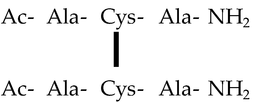
Neutral internal Cys-Cys bond (Ac-Ala-Cys-Ala-NH2)2
All MD simulations were performed with the GROMACS 2022 software package using the CHARMM36m force field parameters with the CHARMM36m consistent version of TIP3Pm water. [22,23,43,44,45,46,47,48,49,50,51,52,53] Peptides were solvated in dodecahedral boxes with TIP3Pm water with 150 mM NaCl.[19] Additional Cl– and Na+ ions were used to neutralize the charges of the systems. The minimum distance of the peptide to the edge of the dodecahedron was 1.4 nm. The solvated conformations were prepared for simulation using a modified protocol of Roe et al. [54] The particle mesh Ewald method was used to calculate long-range electrostatic and van der Waals interactions with cutoff distances of 1.2 nm, and a Fourier spacing was 0.15 nm.[24,25] Initial velocities were assigned to the solvent and peptide separately using a temperature dependent Maxwell-Boltzmann distribution unless otherwise specified.[55,56] The simulation protocol is given below:
- Energy-minimized with 5000 steps of steepest descent with strong positional restraints to the heavy atoms of the peptide, 209.29 kJ/mol/nm with the initial coordinates as a reference.
- 1000 ps of constant volume and temperature (NVT) MD with a weakly coupled Berendsen thermostat with τ=0.5 ps, a 1 fs time-step and strong positional restraints to the heavy atoms of the peptide, 209.29 kJ/mol/nm with initial coordinates as a reference.[57]
- Energy-minimized with 5000 steps of steepest descent with medium positional restraints to the heavy atoms of the peptide, 83.72 kJ/mol/nm with the initial coordinates as a reference.
- Energy-minimized with 5000 steps of steepest descent with weak positional restraints to the heavy atoms of the peptide, 4.19 kJ/mol/nm with the initial coordinates as a reference.
- Energy-minimized with 5000 steps of steepest descent without any positional restraints to the peptide.
- 100 ps of constant pressure and temperature (NPT) MD with a weakly coupled Berendsen thermostat and barostat with τ=1.0 ps, 1 fs time-step and medium positional restraints to the heavy atoms of the peptide, 83.72 kJ/mol/nm with the final energy minimized conformation as a reference. Initial velocities will be assigned using a Maxwell-Boltzmann distribution. The hydrogen atoms are restrained by the SHAKE algorithm.[58]
- 100 ps of constant pressure and temperature (NPT) MD with a weakly coupled Berendsen thermostat and barostat with τ=1.0 ps, 1 fs time-step and medium positional restraints to the heavy atoms of the peptide, 20.93 kJ/mol/nm with the final energy minimized conformation as a reference. Initial velocities should be the final velocities from step 6. The hydrogen atoms are restrained by the SHAKE algorithm.
- 100 ps of constant pressure and temperature (NPT) MD with a weakly coupled Berendsen thermostat and barostat with τ=1.0 ps, 1 fs time-step and medium positional restraints to the heavy atoms of the peptide, 4.19 kJ/mol/nm with the final energy minimized conformation as a reference. Initial velocities should be the final velocities from step 7. The hydrogen atoms are restrained by the SHAKE algorithm.
- 100 ps of constant pressure and temperature (NPT) MD with a weakly coupled Berendsen thermostat and barostat with τ=1.0 ps, 2 fs time-step and without restraints to the heavy atoms of the peptide. Initial velocities should be the final velocities from step 8. The hydrogen atoms are restrained by the SHAKE algorithm.
Production run of 1.0 μs NPT simulations performed at 310 K and 101.325 kPa pressure. The peptide and solvent with ions were separately coupled to a Parrinello-Rahman barostats and the temperatures were maintained by separate coupling to stochastic thermostats using the velocity-rescaling method of Bussi-Parrinello.[59,60] The LINCS algorithm will be used to constrain all bonds to their correct length, with a warning angle of 30°.[61,62] For analysis, a sampling frequency of 0.1 ns was utilized.
Trajectories were sampled for analysis after the system density reached a plateau.[54] An essential dynamics analysis of the trajectory was also be performed.[63,64,65] The covariance matrix for the backbone peptide atoms (-N-Cα-C-) was calculated using the covar module of GROMACS, the eigenvectors corresponding to the 10 highest eigenvalues were used to calculate the backbone configurational entropy as a function of time. This value also plateaued prior to trajectory sampling.
The time dependent ϕ,ψ dihedral angles of the central Xaa residue were extracted from the trajectories using the rama utility of GROMACS, and an in-house Python script.[66] The three-dimensional binned histograms of the normalized density were created for the ϕ,ψ dihedrals of Xaa with one degree of resolution using an R script and plotted using the MatPlotLib package in Python.[60,61,62,63,64,65,66,67] Contours representing the 98% and 99.8% of the sampled populations were generated using the smoothing algorithm of Lovell et al. and calculated using KIN2DCONT.[26,70] The ϕ,ψ dihedrals of Xaa for each peptide were subsequently grouped into their respective β, α, αL, ε, and contiguous regions of ϕ,ψ space using density clustering methodology as implemented in DBSCAN within the Scikit Learn package for Python.[66,70,71,72,73] The minimum cluster size for DBSCAN was 1000 conformations within a 10° radius. To account for the periodicity of the ϕ,ψ dihedral angles, clustering was performed in both the -180° to +180° and 0° to 360° representations of ϕ,ψ space then deconvoluted using an inhouse PERL script to remove redundant data points from each cluster.[74] Sample proportions (ρ) and standard deviations (σ) for each population of β, α, αL, ε, and contiguous regions of ϕ,ψ space of the Xaa residues of each peptide were calculated.[75] The sum of the probabilities for each Ac-Ala-Xaa-Ala-NH2 system are such that;
there are k groups representing the β, α, αL, ε, and contiguous regions and the total population size (nTot) is calculated as
where k and are defined above. The standard deviation of each ρι is,
Statistical comparisons within each region of ϕ,ψ space (β, α, αL, ε, and contiguous) were performed using two-tailed χ2-test.
k is the number of groups being compared (the number of filled entries in a column of Table 1 minus any excluded residues), is the observed value and is the expected value.[75,76] An example data table is given below.

| Category | Xaa | Xaai+1 | … | Xaak | Totals |
|---|---|---|---|---|---|
| β, α, αL, or contig. | Oi | Oi+1 | … | Oi=k | Oi,Total |
| Other | Oj | Oj+1 | … | Oj=k | Oj,Total |
| Oi,j,Total |
The expected value represents the observed value corrected to the weighted arithmetic mean of the observed values:
and
Results are considered statistically significant (the null hypothesis is rejected) if,
where , is the critical value with a significance level of α (α = 0.0001 for this study), and k-1 degrees of freedom.
Individual differences were deconvoluted using the Marascuillo procedure as implemented in R.[67,76,77,78,79] The methodology allows for the simultaneous comparison of all pairs of proportions when multiple populations are being tested. For a system of k populations, the number of unique pairs can be calculated from the binomial theorem.[75]
which can be shown to simplify to:
The critical value is calculated after choosing a significance level,
and using the proportions, and , which are equal to
The absolute difference between proportions, and , is compared to the critical value, , if the relationship between the two is such that,
the null hypothesis is rejected and there is a statistically significant difference between the two pairs with a significance level of α. Results were considered statistically significant if the p-value < 0.0001.
The solvent accessible surface areas (SASA) of each β, α, αL, ε, and contiguous region of ϕ,ψ space for the Xaa residue were calculated using the FreeSASA program with the atomic radii of Tsai et al. a water probe radius of 0.14 nm, 162000 points per sphere and the surface area algorithm of Lee and Richards.[13,41,80] Results were partitioned into whole residue, backbone, and side chain values and the mean and standard deviation for each SASA value were then calculated using the NumPy package for Python.[81] Statistical comparisons between and across Xaa residues were then performed using a Welch’s ANOVA as implemented in the Pingouin package for Python.[31,39,82] The Welch’s ANOVA is utilized due to the variation in β, α, αL, ε and contiguous population sizes and lack of similar variances within the sampled ϕ,ψ dihedral angles for each residue caused a lack of homoscedasticity within the data sets. The f-statistic () for the Welch’s ANOVA is expressed as,
k is the number groups being analyzed, is the size of the population within each group, and the variances are weighted as follows,
is the variance of each population i. The sum of all variances is given as:
The critical value of F is calculated with a value of significance (1 - α; α = 0.0001 in this study) and modified () and () degrees of freedom.
The null hypothesis is rejected if the following relationship holds true.
values were considered statistically significant if the p-value <0.0001.[31,39,83,84] A pairwise difference between residues was compared using Scheffe’s method.[85] The number of possible pairwise relationships are the same as the Marascuillo procedure discussed above. The test statistic is calculated as,
k is the number of groups within the ANOVA analysis, is the f-statistic calculated from the ANOVA, and are the respective sizes of the populations being compared and MSE is the mean squared error.
The null hypothesis is rejected if the absolute difference between the means of the two pairs being compared (i and j) is greater than .
All utilized Python packages required the use of the Pandas package for importation and data organization.[86]
6. Conclusions
The ϕ,ψ space sampling of the Xaa residues within the Ac-Ala-Xaa-Ala-NH2 system simulated at physiologic temperatures (310 K (37° C)), and salt concentrations (150 mM NaCl) presented herein, most likely represents a realistic model of short peptides within solution. The Ac-Ala-Xaa-Ala-NH2 peptides exist as an ensemble of conformations with the ϕ,ψ dihedrals of the central Xaa residues favoring the β region of ϕ,ψ space without the presence of secondary structure or significant hydrogen bond formations. Major conclusions of the present work are:
• Subtle differences in amino acid charge and tautomer state can affect the probability of sampling a particular region of ϕ,ψ space.
• Subtle differences in amino acid charge and tautomer state also effect the mean and standard deviation of the ϕ,ψ dihedral angles for each β, α, αL and ε conformational region.
• Pronounced differences occur in the αL and ε regions as a function of side chain sizes and chemical properties.
• The ε region of ϕ,ψ space is not significantly sampled for multiple amino acids while the αL region is.
• The ε region is accessible to small hydrophobic, and hydrophilic residues (Ala, Ser, Asn, and Asp) but also bulky aromatics (His, Phe, Tyr, and Trp).
• The population density map of each amino acid’s ϕ,ψ space as shown in Figures S1 and S2 is unique and may be affected by the i-1 and i+1 adjacent residues.
• The lack of uniform sampling in the β, α, αL, and ε regions of ϕ,ψ space in the Ace-Ala-Gly-Ala-NH2 system reported here and in contrast to previously published QM/MM results for Ace-Gly-NH2 indicate that the ϕ,ψ dihedral sampling of Gly is affected by the i-1 and i+1 adjacent residues.[27,28]
• Statistically significant differences exist in backbone and side chain SASA comparing β, α, αL, ε, and contiguous regions of ϕ,ψ space.
Supplementary Materials
The following supporting information can be downloaded at the website of this paper posted on Preprints.org: Figure S1. Two-dimensional histograms demonstrating the log10 scaled probabilities (ρ) of the sampled φ,ψ space for the Xaa residues within the Ac-Ala-Xaa-Ala-NH2 peptides. Black contour lines represent 98% of the sampled population, brown contour lines represent 99.8%. Figure S2. Sampled secondary structure classifications for the φ,ψ space for the Xaa residues within the Ac-Ala-Xaa-Ala-NH2 peptides as determined by density clustering. Blue, β, Red, α, Green, αL, Cyan, ε, Purple, contiguous. Table S1. The probability () and number of conformations (n) of the φ,ψ dihedral angles of the Xaa residue within the Ace-Ala-Xaa-Ala-NH2 peptides within the β, α, αL, ε, or contiguous regions of φ,ψ space as assigned by density clustering demonstrated in Figure S2. The results are compared using a χ2-analysis.a,b,c Results are considered statistically significant for an α = 0.0001 using a right-tailed χ2 distribution. Table S2. Statistically significant pairwise comparisons of the probability of the central Xaa residue φ,ψ dihedral angles populating the β conformation region. Table S3. Non-statistically significant pairwise comparisons of the probability of the central Xaa residue φ,ψ dihedral angles populating the β conformation region. Table S4. Statistically significant pairwise comparisons of the probability of the central Xaa residue φ,ψ dihedral angles populating the α conformation region. Table S5. Non-statistically significant pairwise comparisons of the probability of the central Xaa residue φ,ψ dihedral angles populating the α conformation region. Table S6. Statistically significant pairwise comparisons of the probability of the central Xaa residue φ,ψ dihedral angles populating the αL conformation region. Table S7. Non-statistically significant pairwise comparisons of the probability of the central Xaa residue φ,ψ dihedral angles populating the αL conformation region. Table S8. Statistically significant pairwise comparisons of the probability of the central Xaa residue φ,ψ dihedral angles populating the ε conformation region. Table S9. Non-statistically significant pairwise comparisons of the probability of the central Xaa residue φ,ψ dihedral angles populating the ε conformation region. Table S10. Statistically significant pairwise comparisons of the probability of the central Xaa residue φ,ψ dihedral angles populating the contiguous conformation region. Table S11. Non-statistically significant pairwise comparisons of the probability of the central Xaa residue φ,ψ dihedral angles populating the contiguous conformation region. Table S12. The φ,ψ dihedral angles of the Xaa residue within the Ac-Ala-Xaa-Ala-NH2 peptides assigned by density clustering to the β, α, αL, ε, and contiguous regions demonstrated in Figure S2 and expressed as a mean ± standard deviation(degrees). Results are compared using a Welch’s analysis of variance (ANOVA).a,b Results are considered statistically significant for an α = 0.0001 using a right-tailed F distribution. Table S13. Statistically significant pairwise comparisons of the φ dihedral angles populating the β conformation region. Table S14. Non-statistically significant pairwise comparisons of the φ dihedral angles populating the β conformation region. Table S15. Statistically significant pairwise comparisons of the ψ dihedral angles populating the β conformation region. Table S16. Non-statistically significant pairwise comparisons of the ψ dihedral angles populating the β conformation region. Table S17. Statistically significant pairwise comparisons of the φ dihedral angles populating the α conformation region. Table S18. Non-statistically significant pairwise comparisons of the φ dihedral angles populating the α conformation region. Table S19. Statistically significant pairwise comparisons of the ψ dihedral angles populating the α conformation region. Table S20. Non-statistically significant pairwise comparisons of the ψ dihedral angles populating the α conformation region. Table S21. Statistically significant pairwise comparisons of the φ dihedral angles populating the αL conformation region. Table S22. Non-statistically significant pairwise comparisons of the φ dihedral angles populating the αL conformation region. Table S23. Statistically significant pairwise comparisons of the ψ dihedral angles populating the αL conformation region. Table S24. Non-statistically significant pairwise comparisons of the ψ dihedral angles populating the αL conformation region. Table S25. Statistically significant pairwise comparisons of the φ dihedral angles populating the ε conformation region. Table S26. Non-statistically significant pairwise comparisons of the φ dihedral angles populating the ε conformation region. Table S27. Statistically significant pairwise comparisons of the ψ dihedral angles populating the ε conformation region. Table S28: Non-statistically significant pairwise comparisons of the ψ dihedral angles populating the ε conformation region. Table S29. Statistically significant pairwise comparisons of the φ dihedral angles populating the contiguous conformation region. Table S30. Non-statistically significant pairwise comparisons of the φ dihedral angles populating the contiguous conformation region. Table S31. Statistically significant pairwise comparisons of the ψ dihedral angles populating the contiguous conformation region. Table S32. Non-statistically significant pairwise comparisons of the ψ dihedral angles populating the contiguous conformation region. Table S33. The mean standard ± deviation distances between the i-1 (Ala 1) carbonyl oxygen and i+1 (Ala 3) amide nitrogen of the Ac-Ala-Xaa-Ala-NH2 peptides. The probability () and number of conformations (n) with distances between 0.27 and 0.33 nm indicating possible hydrogen bond formation. Table S34. The mean standard ± deviation distances between the i-1 (Ala 1) amide nitrogen and i+1 (Ala 3) carbonyl oxygen of the Ac-Ala-Xaa-Ala-NH2 peptides. The probability () and number of conformations (n) with distances between 0.27 and 0.33 nm indicating possible hydrogen bond formation. Table S35. The solvent accessible surface area (SASA) for the whole Xaa residue of Ac-Ala-Xaa-Ala-NH2 as a function of β, α, αL, ε, and contiguous regions of φ,ψ space assigned by density clustering and demonstrated in Figure S2. Results are compared using a Welch’s analysis of variance (ANOVA).a,b Results are considered statistically significant for an α = 0.0001 using a right-tailed F distribution. Table S36. The solvent accessible surface area (SASA) for the Xaa residue backbone of Ac-Ala-Xaa-Ala-NH2 as a function of β, α, αL, ε, and contiguous regions of φ,ψ space assigned by density clustering and demonstrated in Figure S2. Results are compared using a Welch’s analysis of variance (ANOVA).a,b Results are considered statistically significant for an α = 0.0001 using a right-tailed F distribution. Table S37. The solvent accessible surface area (SASA) for the Xaa residue side chain of Ac-Ala-Xaa-Ala-NH2 as a function of β, α, αL, ε, and contiguous regions of φ,ψ space assigned by density clustering and demonstrated in Figure S2. Results are compared using a Welch’s analysis of variance (ANOVA).a,b,c Results are considered statistically significant for an α = 0.0001 using a right-tailed F distribution. Table S38. Scheffe’s pairwise comparison of the solvent accessible surface area (SASA) for the whole Xaa residue of Ac-Ala-Xaa-Ala-NH2 as a function of β, α, αL, ε, and contiguous regions of φ,ψ dihedral space assigned by density clustering and demonstrated in Figure S2. Table S39. Scheffe’s pairwise comparison of the solvent accessible surface area (SASA) for the backbone Xaa residue of Ac-Ala-Xaa-Ala-NH2 as a function of β, α, αL, ε, and contiguous regions of φ,ψ dihedral space assigned by density clustering and demonstrated in Figure S2. Table S40. Scheffe’s pairwise comparison of the solvent accessible surface area (SASA) for the side chain Xaa residue of Ac-Ala-Xaa-Ala-NH2 as a function of β, α, αL, ε, and contiguous regions of φ,ψ dihedral space assigned by density clustering and demonstrated in Figure S2.
Author Contributions
Conceptualization, C.R.W. and S.L..; methodology, C.R.W; software, W.A.B. and C.R.W.; validation, C.R.W. and S.L.; formal analysis, W.A.B. and C.R.W.; investigation, W.A.B.; resources, C.R.W.; data curation, W.B.; writing—original draft preparation, W.A.B. and C.R.W; writing—review and editing, C.R.W. and S.L.; visualization, W.A.B.; supervision, C.R.W.; project administration, C.R.W..; funding acquisition, C.R.W. All authors have read and agreed to the published version of the manuscript.
Funding
This research was funded by the Park Nicollet Foundation; Dr. A. Reginald and Anna Watts Neurosurgical/Neuroscience Research Fund. S.L was supported by National Institutes of Health R01 CA253573-01 and the state of Nebraska LB595 grants.
Institutional Review Board Statement
Not applicable.
Informed Consent Statement
Not applicable.
Data Availability Statement
The original data (Simulation time; SASA-whole residue; SASA-backbone; SASA-side chain; ϕ dihedral angle; ψ dihedral angle; amino acid; and β, α, αL, ε, and contiguous cluster assignment and smoothed distribution surfaces) presented in this study are openly available in ZENODO at DOI: 10.5281/zenodo.13137464.
Conflicts of Interest
Charles R. Watts is a consultant for Medtronic Spine and Biologics and Thompson Surgical Instruments. The remaining authors have disclosed that they do not have any conflicts of interest. The funders had no role in the design of the study; in the collection, analyses, or interpretation of data; in the writing of the manuscript, or in the decision to publish the results.
Appendix A
Assignments of Force Field Parameters for L-α-Tyrosine and L-α-Arginine base Residues.
The Lennard-Jones, electrostatic potentials, bond, bond angle, and torsional parameters for the Tyr-, Arg:NH, and Arg:NE residues were assigned based on the similarity and transferability of force field parameters for the phenol base for Tyr- and methyl guanidine for Arg:NH and Arg:NE within the CHARMM36m force field using the same methodology as the CGenFF program while taking care to use the appropriate backbone dihedral and CMAP potentials.[22,43,44,45,46,87,88,89,90,91] The following lines were added to the merged.rtp file in the charmm36-ljpme-jul2021.ff directory tree of GROMACS. Standard CMAP potentials were used for the ϕ,ψ dihedral angles and no modifications were made to the cmap.itp file within the charmm36-ljpme-jul2021.ff directory.
#aminoacids.rtp
[ TYRN ]
;
[ atoms ]
N NH1 -0.4700 1
HN H 0.3100 1
CA CT1 0.0700 1
HA HB1 0.0900 1
CB CT2 -0.1800 2
HB1 HA2 0.0900 2
HB2 HA2 0.0900 2
CG CA 0.0000 3
CD1 CA -0.1150 4
HD1 HP 0.1150 4
CE1 CA -0.5990 5
HE1 HP 0.2800 5
CZ CA 0.4000 6
OH OG312 -0.7620 6
CD2 CA -0.1150 7
HD2 HP 0.1150 7
CE2 CA -0.5990 8
HE2 HP 0.2800 8
C C 0.5100 9
O O -0.5100 9
[ bonds ]
CB CA
CG CB
CD2 CG
CE1 CD1
CZ CE2
OH CZ
N HN
N CA
C CA
C +N
CA HA
CB HB1
CB HB2
CD1 HD1 15
CD2 HD2
CE1 HE1
CE2 HE2
O C
CD1 CG
CE1 CZ
CE2 CD2
[ impropers ]
N -C CA HN
C CA +N O
[ cmap ]
-C N CA C +N
#
#aminoacids.hdb
TYRN 7
1 1 HN N CA -C
1 5 HA CA N CB C
2 6 HB CB CG CA
1 1 HD1 CD1 CE1 CG
1 1 HE1 CE1 CD1 CZ
1 1 HD2 CD2 CG CE2
1 1 HE2 CE2 CZ CD2
#
#ffbonded.itp
; i j func b0 kb
CA OG312 1 0.12600000 439320.00
; i j k func theta0 ktheta ub0 kub
CA CA OG312 5 120.000000 334.720000 0.00000000 0.00
; i j k l func phi0 kphi mult
CA CA CA OG312 9 180.000000 12.970400 2
; i j k l func phi0 kphi mult
OG312 CA CA HP 9 180.000000 10.041600 2
#
#aminoacids.rtp
[ ARGN1]; Isomer 1:unprotonated NE nitrogen
;
[ atoms ]
N NH1 -0.4700 1
HN H 0.3100 1
CA CT1 0.0700 1
HA HB1 0.0900 1
CB CT2 -0.1800 2
HB1 HA2 0.0900 2
HB2 HA2 0.0900 2
CG CT2 -0.1800 3
HG1 HA2 0.0900 3
HG2 HA2 0.0900 3
CD CT2 0.0600 4
HD1 HA2 0.0900 4
HD2 HA2 0.0900 4
NE NG2D1 -0.8600 4
CZ CG2N1 0.6600 4
NH1 NG321 -0.6000 4
HH11 HGPAM2 0.2900 4
HH12 HGPAM2 0.2900 4
NH2 NG321 -0.6000 4
HH21 HGPAM2 0.2900 4
HH22 HGPAM2 0.2900 4
C C 0.5100 5
O O -0.5100 5
[ bonds ]
CB CA
CG CB
CD CG
NE CD
CZ NE
NH2 CZ
N HN
N CA
C CA
C +N
CA HA
CB HB1
CB HB2
CG HG1
CG HG2
CD HD1
CD HD2
NH1 HH11
NH1 HH12
NH2 HH21
NH2 HH22
O C
CZ NH1
[ impropers ]
N -C CA HN
C CA +N O
CZ NH1 NH2 NE
[ cmap ]
-C N CA C +N
#
#aminoacids.hdb
ARGN 7
1 1 HN N CA -C
1 5 HA CA N CB C
2 6 HB CB CG CA
2 6 HG CG CB CD
2 6 HD CD CG NE
2 3 HH1 NH1 CZ NH2
2 3 HH2 NH2 CZ NH1
#
# ffbonded.itp entries
; i j func b0 kb
CT2 NG2D1 1 0.14400000 245182.40
; i j k func theta0 ktheta ub0 kub
CT2 CT2 NG2D1 5 112.000000 861.904000 0.00000000 0.00
NG2D1 CT2 HA2 5 107.500000 376.560000 0.00000000 0.00
CG2N1 NG2D1 CT2 5 108.000000 418.400000 0.00000000 0.00
; i j k l func phi0 kphi mult
NG321 CG2N1 NG2D1 CT2 9 180.000000 27.196000 2
HA2 CT2 NG2D1 CG2N1 9 180.000000 0.460240 3
CT2 CT2 NG2D1 CG2N1 9 0.000000 0.418400 3
; i j k l func phi0 kphi
NG321 HGPAM2 HGPAM2 CG2N1 2 180.000000 711.280000
#
#aminoacids.rtp
[ ARGN2]; Isomer 2: protonated NE nitrogen
;
[ atoms ]
N NH1 -0.4700 1
HN H 0.3100 1
CA CT1 0.0700 1
HA HB1 0.0900 1
CB CT2 -0.1800 2
HB1 HA2 0.0900 2
HB2 HA2 0.0900 2
CG CT2 -0.1800 3
HG1 HA2 0.0900 3
HG2 HA2 0.0900 3
CD CT2 -0.1100 4
HD1 HA2 0.0900 4
HD2 HA2 0.0900 4
NE NG2D1 -0.5400 4
HE H 0.3600 4
CZ CG2N1 0.5900 4
NH1 NG321 -0.9100 4
HH11 HGPAM1 0.3700 4
NH2 NG321 -0.6000 4
HH21 HGPAM2 0.3300 4
HH22 HGPAM2 0.3300 4
C C 0.5100 5
O O -0.5100 5
[ bonds ]
CB CA
CG CB
CD CG
NE CD
CZ NE
NH2 CZ
N HN
N CA
C CA
C +N
CA HA
CB HB1
CB HB2
CG HG1
CG HG2
CD HD1
CD HD2
NE HE
NH1 HH11
NH2 HH21
NH2 HH22
O C
CZ NH1
[ impropers ]
N -C CA HN
C CA +N O
CZ NH1 NH2 NE
[ cmap ]
-C N CA C +N
#
#aminoacids.hdb
ARGN 8
1 1 HN N CA -C
1 5 HA CA N CB C
2 6 HB CB CG CA
2 6 HG CG CB CD
2 6 HD CD CG NE
1 1 HE NE CZ CD
1 2 HH11 NH1 CZ NH2
2 3 HH2 NH2 CZ NH1
#
#ffbonded.itp
; i j func b0 kb
CT2 NG2D1 1 0.14400000 245182.40
H NG2D1 1 0.10000000 380744.00
NG321 HGPAM1 1 0.10200000 379907.20
; i j k func theta0 ktheta ub0 kub
CT2 CT2 NG2D1 5 112.000000 861.904000 0.00000000 0.00
NG2D1 CT2 HA2 5 107.500000 376.560000 0.00000000 0.00
CG2N1 NG2D1 H 5 113.000000 410.032000 0.00000000 0.00
CG2N1 NG321 HGPAM1 5 113.000000 410.032000 0.00000000 0.00
CT2 NG2D1 H 5 104.000000 376.560000 0.00000000 0.00
CT2 NG2D1 CG2N1 5 108.000000 418.400000 0.00000000 0.00
; i j k l func phi0 kphi mult
CT2 CT2 NG2D1 H 9 180.000000 1.255200 3
NG2D1 CG2N1 NG321 HGPAM1 9 180.000000 21.756800 2
NG321 CG2N1 NG321 HGPAM1 9 180.000000 21.756800 2
HA2 CT2 NG2D1 CG2N1 9 180.000000 0.000000 3
CT2 NG2D1 CG2N1 NG321 9 180.000000 2.092000 2
H NG2D1 CG2N1 NG321 9 180.000000 11.715200 3
HA2 CT2 NG2D1 H 9 0.000000 1.75728 3
CT2 CT2 NG2D1 CG2N1 9 180.000000 2.59408 2
#
Figure A1.
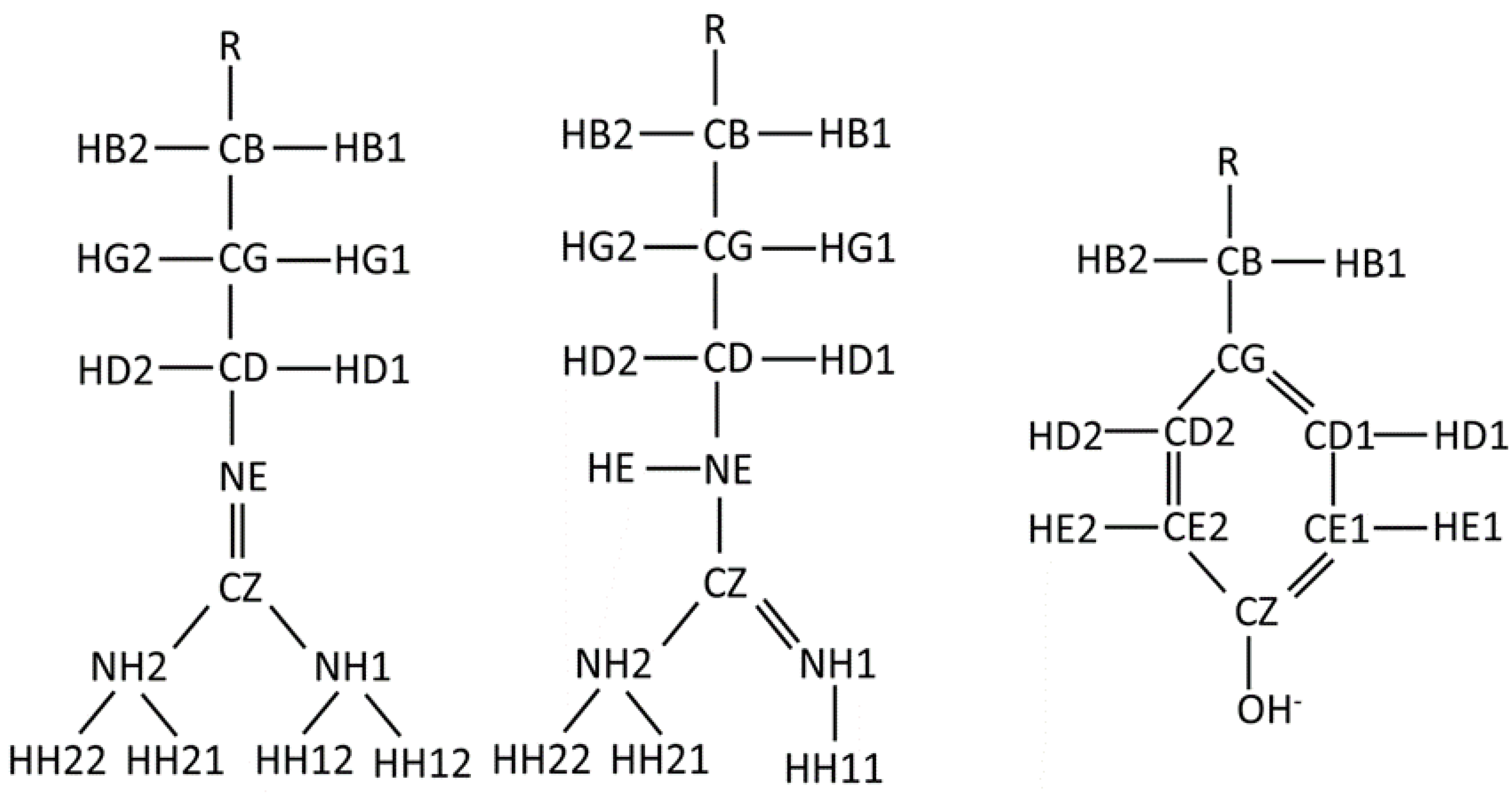
Simplified diagrams of the Tyr-, Arg:NH and Arg:NE side chains demonstrating the atom names used for the residue. R represents the backbone of the amino acid residue.
Figure A1.
Simplified diagrams of the Tyr-, Arg:NH and Arg:NE side chains demonstrating the atom names used for the residue. R represents the backbone of the amino acid residue.
References
- wwPDB Consortium. Protein Data Bank: the single global archive for 3D macromolecular structure data. Nucleic Acids Res. 2019, 47 (D1), D520-D528.
- Klebl, D.P.; Aspinall, L.; Muench, S.P. Time resolved applications for Cryo-EM; approaches, challenges and future directions. Curr Opin Struct Biol. 2023, 83, 102696. [Google Scholar]
- Raviv, U.; Asor, R.; Shemesh, A.; Ginsburg, A.; Ben-Nun, T.; Schilt, Y.; Levartovsky, Y.; Ringel, I. Insight into structural biophysics from solution X-ray scattering. J Struct Biol. 2023, 215(4), 108029. [Google Scholar] [CrossRef] [PubMed]
- Hekstra, D.R. Emerging Time-Resolved X-Ray Diffraction Approaches for Protein Dynamics. Annu Rev Biophys. 2023, 9, 255–274. [Google Scholar] [CrossRef] [PubMed]
- Zadorozhnyi, R.; Gronenborn, A.M.; Polenova, T. Integrative approaches for characterizing protein dynamics: NMR, CryoEM, and computer simulations. Curr Opin Struct Biol. 2023, 84, 102736. [Google Scholar]
- Arthanari, H.; Takeuchi, K.; Dubey, A.; Wagner, G. Emerging solution NMR methods to illuminate the structural and dynamic properties of proteins. Curr Opin Struct Biol. 2019, 58, 294–304. [Google Scholar] [CrossRef] [PubMed]
- Ceruso, M.A.; Amadei, A.; Di Nola, A. Mechanics and dynamics of B1 domain of protein G: role of packing and surfacce hydrophobic residues. Protein Sci. 1999, 8(1), 147–160. [Google Scholar] [CrossRef] [PubMed]
- Kmiecik, S.; Kolinski, A. Folding pathway of the B1 domain of Protein G explored by mulitiscale modeling. Biophys J. 2008, 94(3), 726–736. [Google Scholar] [CrossRef] [PubMed]
- Moult, J.; Pedersen, J.T.; Judson, R.; Fidelis, K. A large-scale experiment to assess protein structure prediction methods. Proteins 1995, 23(3), ii–iV. [Google Scholar]
- Jumper, J.; Evans, R.; Pritzel, A.; Green, T.; Figurnov, M.; Ronneberger, O.; Tunyasuvunakool, K.; Bates, R.; Žídek, A.; Potapenko, A.; Bridgland, A.; Meyer, C.; Kohl, S.A.A.; Ballard, A.J.; Cowie, A.; Romera-Paredes, B.; Nikolov, S.; Jain, R.; Adler, J.; Back, T.; Petersen, S.; Reiman, D.; Clancy, E.; Zielinski, M.; Steinegger, M.; Pacholska, M.; Berghammer, T.; Bodenstein, S.; Silver, D.; Vinyals, O.; Senior, A.W.; Kavukcuoglu, K.; Kohli, P.; Hassabis, D. Highly accurate protein structure prediction with AlphaFold. Nature 2021, 596(7873), 583–589. [Google Scholar] [CrossRef]
- Abramson, J.; Adler, J.; Dunger, J.; Evans, R.; Green, T.; Pritzel, A.; Ronneberger, O.; Willmore, L.; Ballard, A.J.; Bambrick, J.; Bodenstein, S.W.; Evans, D.A.; Hung, C.-C.; O’Neill, M.; Reiman, D.; Tunyasuvunakool, K.; Wu, Z.; Žemgulytė, A.; Arvaniti, E.; Beattie, C.; Bertolli, O.; Bridgland, A.; Cherepanov, A.; Congreve, M.; Cowen-Rivers, A.I.; Cowie, A.; Figurnov, M.; Fuchs, B.; Gladman, H.; Jain, R.; Khan, Y.A.; Low, C.M.R.; Perlin, K.; Potapenko, A.; Savy, P.; Singh, S.; Stecula, A.; Thillaisundaram, A.; Tong, C.; Yakneen, S.; Zhong, E.D.; Zielinski, M.; Žídek, A.; Bapst, V.; Kohli, P.; Jaderberg, M.; Hassabis, D.; Jumper, J.M. Accurate structure prediction of biomolecular interactions with AlphaFold 3. Nature 2024, 630(8016), 493–500. [Google Scholar] [CrossRef]
- Shaytan, A.K.; Shaitan, K.V.; Khokhlov, A.R. Solvent accessible surface area of amino acid residues in globular proteins: correlation of apparent transfer free energies with experimental hydrophobicity scales. Biomacromolecules 2009, 10(5), 1224–1237. [Google Scholar] [CrossRef]
- Lee, B.; Richards, F.M. The interpretation of protein structures: estimation of static accessibility. J Mol Biol. 1971, 55, 379–400. [Google Scholar] [CrossRef] [PubMed]
- Miller, S.; Janin, J.; Lesk, A.M.; Chothia, C. Interior and surface of monomeric proteins. J Mol Biol. 1987, 196, 641–656. [Google Scholar] [PubMed]
- Harpaz, Y.; Gerstein, M.; Chothia, C. Volume changes on protein folding. Structure 1994, 2(7), 641–649. [Google Scholar] [CrossRef]
- Carugo, O. Amino acid composition and protein dimension. Protein Sci. 2008, 17(12), 2187–2191. [Google Scholar] [CrossRef]
- Zielenkiewicz, P.; Saenger, W. Residue solvent accessibilities in the unfolded polypeptide chain. Biophys J. 1992, ‘63 (6), 1483-1486.
- Maple, J.R.; Dinur, U.; Hagler, A.T. Derivation of force fields for molecular mechanics and dynamics from ab initio energy surfaces. Proc Natl Acad Sci U S A 1988, 85(15), 5350–5354. [Google Scholar] [CrossRef]
- Ibragimova, G.T.; Wade, R.C. Importance of explicit salt ions for protein stability in molecular dynamics simulation. Biophys J. 1998, 74(11), 2906–2911. [Google Scholar] [CrossRef]
- Tien, M.Z.; Meyer, A.G.; Sydykova, D.K.; Spielman, S.J.; Wilke, C.O. Maximum Allowed Solvent Accessibilities of Residues in Proteins. PLOS ONE 2013, 8, e80635. [Google Scholar]
- Topham, C.M.; Smith, J.C. Tri-peptide reference structures for the calculation of relative solvent accessible surface area in protein amino acid residues. CComput Biol Chem. 2015, 54, 33–43. [Google Scholar] [PubMed]
- Huang, J.; Rauscher, S.; Nawrocki, G.; Ran, T.; Feig, M.; de Groot, B.L.; Grubmüller, H.; MacKerell, A.D.J. CHARMM36m: an improved force field for folded and intrinsically disordered proteins. Nature Methods 2017, 14(1), 71–73. [Google Scholar] [CrossRef]
- Abraham, M.J.; van der Spoel, D.; Lindahl, E.; Hess, B. http://www.gromacs.org, 2022. Gromacs. http://www.gromacs.org (accessed June 1, 2022).
- Essmann, U.; Perera, L.; Berkowitz, M.L.; Darden, T.; Lee, H.; Pedersen, L.G. A smooth particle mesh Ewald method. Journal Chem Phys. 1995, 103(19), 8577–8593. [Google Scholar] [CrossRef]
- Wennberg, C.L.; Murtola, T.; Hess, B.; Lindahl, E. Lennard-Jones Lattice Summation in Bilayer Simulations Has Critical Effects on Surface Tension and Lipid Properties. Journal of Chemical Theory and Computation 2013, 9(8), 3527–3537. [Google Scholar] [CrossRef] [PubMed]
- Lovell, S.C.; Davis, I.W.; Arendall III, W.B.; de Bakker, P.I.W.; Word, J.M.; Prisant, M.G.; Richardson, J.S.; Richardson, D.C. Structure validation by Cα geometry: ϕ,ψ and Cβ deviation. Proteins: Structure, Function, and Bioinformatics 2003, 50 (3), 437-450.
- Ho, B.K.; Brasseur, R. The Ramachandran plots of glycine and pre-proline. BMC Struct Biol. 2005, 5, 14. [Google Scholar]
- Hu, H.; Elstner, M.; Hermans, J. Comparison of a QM/MM force field and molecular mechanics force fields in simulations of alanine and glycine “dipeptides” (Ace-Ala-Nme and Ace-Gly-Nme) in water in relation to the problem of modeling the unfolded peptide backbone in solution. Proteins. 2003, 50(3), 451–463. [Google Scholar] [CrossRef] [PubMed]
- Craveur, P.; Joseph, A.P.; Poulain, P.; de Brevern, A.G.; Rebehmed, J. Cis-trans isomerization of omega dihedrals in proteins. Amino Acids 2013, 45(2), 279–289. [Google Scholar] [CrossRef] [PubMed]
- Yonezawa, Y.; Nakata, K.; Sakakura, K.; Takada, T.; Nakamura, H. Intra- and intermolecular interaction inducing pyramidalization on both sides of a proline dipeptide during isomerization: an ab initio QM/MM molecular dynamics simulation study in explicit water. J Am Chem Soc. 2009, 131(12), 4535–4540. [Google Scholar] [CrossRef]
- Welch, B.L. The Generalization of ‘Student’s’ Problem when Several Different Population Variances are Involved. Biometrika 1947, 34 (1/2), 28-35.
- Jeffrey, G.A. An introduction to hydrogen bonding; Oxford University Press: New York, 1997; p. 191,200. [Google Scholar]
- Kabsch, W.; Sander, C. Dictionary of protein secondary structure: pattern recognition of hydrogen-bonded and geometrical features. Biopolymers 1983, 22(12), 2577–2637. [Google Scholar] [CrossRef]
- Bystrov, V.F.; Portnova, S.L.; Tsetlin, V.I.; Ivanov, V.T.; Ovchinnikov, Y.A. Conformational studies of peptide systems. The rotational states of the NH--CH fragment of alanine dipeptides by nuclear magnetic resonance. Tetrahedron 1969, 25 (3), 493-515.
- Milner-White, E.J. Situations of gamma-turns in proteins. Their relation to alpha-helices, beta-sheets and ligand binding sites. J Mol Biol 1990, 216 (2), 386-397.
- Shrake, A.; Rupley, J.A. Environment and exposure to solvent of protein atoms. Lysozyme and insulin. J Mol Biol. 1973, 79, 351–372. [Google Scholar]
- Rose, G.D.; Geselowitz, A.R.; Lesser, G.J.; Lee, R.M.; Zehfus, M.M. Hydrophobicity of amino acid residues in globular proteins. Science 1985, 229, 834–838. [Google Scholar]
- Chothia, C. The nature of the accessible and buried surfaces in proteins. J Mol Biol. 1976, 105, 1–14. [Google Scholar] [CrossRef]
- Welch, B.L. On the comparison of several mean values: an alternative approach. Biometrika. 1951, 38 (3-4), 330-336.
- Student. The Probable Error of a Mean. Biometrika 1908, 6(1), 1–25.
- Tsai, J.; Taylor, R.; Chothia, C.; Gerstein, M. The Packing Density in Proteins: Standard Radii and Volumes. J Mol Biol. 1999, 290, 253–266. [Google Scholar] [CrossRef] [PubMed]
- DeLano, W. Schrödinger LLC. https://www.pymol.com/pymol.
- Best, R.B.; Zhu, X.; Shim, J.; Lopes, P.E.M.; Mittal, J.; Feig, M.; MacKerell, A.D.J. Optimization of the Additive CHARMM All-Atom Protein Force Field Targeting Improved Sampling of the Backbone ϕ, ψ and Side-Chain χ1 and χ2 Dihedral Angles. J Chem Theory Comput. 2012, 8(9), 3257–3273. [Google Scholar] [CrossRef] [PubMed]
- Mackerell, A.D.J.; Feig, M.; Brooks, C.L.I. Extending the treatment of backbone energetics in protein force fields: Limitations of gas-phase quantum mechanics in reproducing protein conformational distributions in molecular dynamics simulations. Journal of Computational Chemistry 2004, 25(11), 0192–8651. [Google Scholar]
- MacKerell Jr., A. D.; Bashford, D.; Bellott, M.; Dunbrack Jr., R.L.; Evanseck, J.D.; Field, M.J.; Fischer, S.; Gao, J.; Guo, H.; Ha, S.; Joseph-McCarthy, D.; Kuchnir, L.; Kuczera, K.; Lau, F.T.K.; Mattos, C.; Michnick, S.; Ngo, T.; Nguyen, D.T.; Prodhom, B.; Reiher, W.E.; Roux, B.; Schlenkrich, M.; Smith, J.C.; Stote, R.; Straub, J.; Watanabe, M.; Wiórkiewicz-Kuczera, J.; Yin, D.; Karplus, M. All-Atom Empirical Potential for Molecular Modeling and Dynamics Studies of Proteins. The Journal of Physical Chemistry B 1998, 102 (18), 3586-3616.
- Vanommeslaeghe, K.; Hatcher, E.; Acharya, C.; Kundu, S.; Zhong, S.; Shim, J.; Darian, E.; Guvench, O.; Lopes, P.; Vorobyov, I.; Mackerell, A.D.J. CHARMM general force field: A force field for drug-like molecules compatible with the CHARMM all-atom additive biological force fields. J Comp Chem. 2010, 31(4), 671–690. [Google Scholar] [CrossRef] [PubMed]
- Abraham, M.J.; Murtola, T.; Schulz, R.; Páll, S.; Smith, J.C.; Hess, B.; Lindahl, E. GROMACS: High performance molecular simulations through multi-level parallelism from laptops to supercomputers. SoftwareX 2015, 1-2, 19-25.
- Páll, S.; Abraham, M.J.; Kutzner, C.; Hess, B.; Lindahl, E.; Markidis, S.; Laure, E. Tackling Exascale Software Challenges in Molecular Dynamics Simulations with GROMACS. Solving Software Challenges for Exascale, Stockholm, 2015; pp 3-27.
- Hess, B.; Kutzner, C.; van der Spoel, D.; Lindahl, E. GROMACS 4: Algorithms for Highly Efficient, Load-Balanced, and Scalable Molecular Simulation. J Chem Theory Comput. 2008, 4(3), 435–447. [Google Scholar] [CrossRef] [PubMed]
- Van Der Spoel, D.; Lindahl, E.; Hess, B.; Groenhof, G.; Mark, A.E.; Berendsen, H.J.C. GROMACS: Fast, flexible, and free. J Comp Chem. 2005, 26(16), 1701–1718. [Google Scholar] [CrossRef] [PubMed]
- Lindahl, E.; Hess, B.; van der Spoel, D. GROMACS 3.0: a package for molecular simulation and trajectory analysis. Molecular modeling annual 2001, 7(8), 306–317. [Google Scholar] [CrossRef]
- Berendsen, H.J.C.; van der Spoel, D.; van Drunen, R. GROMACS: A message-passing parallel molecular dynamics implementation. Comput Phys Commun. 1995, 91(1), 43–56. [Google Scholar] [CrossRef]
- Bjelkmar, P.; Larsson, P.; Cuendet, M.A.; Hess, B.; Lindahl, E. Implementation of the CHARMM Force Field in GROMACS: Analysis of Protein Stability Effects from Correction Maps, Virtual Interaction Sites, and Water Models; J Chem Theory Comput. 2010, 6(2), 459–466. [Google Scholar] [CrossRef]
- Roe, D.R.; Brooks, B.R. A protocol for preparing explicitly solvated systems for stable molecular dynamics simulations. J Chem. Phys. 2020, 153(5), 054123. [Google Scholar] [CrossRef]
- Hoover, W.G. Canonical dynamics: Equilibrium phase-space distributions. Physical Review A 1985, 31(3), 1695–1697. [Google Scholar] [CrossRef]
- Hoover, W.G. Constant-pressure equations of motion. Physical Review A 1986, 34(3), 2499–2500. [Google Scholar] [CrossRef] [PubMed]
- Berendsen, H.J.C.; Postma, J.P.M.; van Gunsteren, W.F.; DiNola, A.; Haak, J.R. Molecular dynamics with coupling to an external bath. J Chem Phys. 1984, 81(8), 3684–3690. [Google Scholar] [CrossRef]
- Ryckaert, J.-P.; Ciccotti, G.; Berendsen, H.J.C. Numerical integration of the cartesian equations of motion of a system with constraints: molecular dynamics of n-alkanes. J Comput Phys. 1977, 23(3), 327–341. [Google Scholar] [CrossRef]
- Parrinello, M.; Rahman, A. Polymorphic transitions in single crystals: A new molecular dynamics method. J Appl Phys. 1981, 52(12), 7182–7190. [Google Scholar] [CrossRef]
- Bussi, G.; Donadio, D.; Parrinello, M. Canonical sampling through velocity rescaling. J Chem Phys. 2007, 126(1), 014101. [Google Scholar] [CrossRef]
- Hess, B.; Bekker, H.; Berendsen, H.J.C.; Fraaije, J.G.E.M. LINCS: A linear constraint solver for molecular simulations. J Comput Chem. 1997, 18(12), 1463–1472. [Google Scholar] [CrossRef]
- Hess, B. P-LINCS: A Parallel Linear Constraint Solver for Molecular Simulation. J Chem Theory Comput. 2008, 4(1), 116–122. [Google Scholar] [CrossRef]
- Andricioaei, I.; Karplus, M. On the calculation of entropy from covariance matrices of the atomic fluctuations. J Chem Phys. 2001, 115(14), 6289–6292. [Google Scholar] [CrossRef]
- Amadei, A.; Ceruso, M.A.; Di Nola, A. On the convergence of the conformational coordinates basis set obtained by the essential dynamics analysis of proteins’ molecular dynamics simulations. Proteins: Structure, Function, and Bioinformatics 1999, 36 (4), 419-424.
- Hayward, S.; de Groot, B. l.; Kukol, A. Normal Modes and Essential Dynamics. In Molecular Modeling of Proteins; Humana Press: Totowa, 2008; Volume 443, pp. 89–106. [Google Scholar]
- Python Software Foundation. Python.org. https://www.python.org (accessed August 15, 2023).
- R Core Team. The R project for Statistical Computing. https://www.r-project.org (accessed Aug 14, 2023).
- Hunter, J.D. Matplotlib: A 2D Graphics Environment. IEEE 2007, 9, 90–95. [Google Scholar] [CrossRef]
- Eisenhaber, F.; Lijnzaad, P.; Argos, P.; Sander, C.; Scharf, M. The double cubic lattice method: Efficient approaches to numerical integration of surface area and volume and to dot surface contouring of molecular assemblies. J Comput Chem. 1995, 16(3), 273–284. [Google Scholar] [CrossRef]
- Word, J.M. All-atom small probe contact surface analysis: an information-rich description of molecular goodness-of-fit; PhD Thesis; Duke University: Durham, 2000. [Google Scholar]
- Ester, M.; Kriegel, H.P.; Sander, J.; Xiaowei, X. A density-based algorithm for discovering clusters in large spatial databases with noise. 2nd international conference on knowledge discovery and data mining, Portland, 1996.
- Tan, P.N.; Steinbach, M.; Kumar, V. Cluster Analysis Basic Concepts and Algorithms. In Introduction to Data Mining, 2nd ed.; Pearson Addison Wesley: Boston, 2005; pp. 487–568. [Google Scholar]
- Tan, P.N.; Steinbach, M.; Kumar, V. Cluster Analysis Additional Issues and Algorithms. In Introduction to Data Mining, 2nd ed.; Pearson Addison Wesley: Boston, 2005; pp. 569–650. [Google Scholar]
- The Perl Foundation. Perl Website. https://www.perl.org (accessed August 30, 2023).
- Navidi, W. The Binomial Distribution. In Statistics for Engineers and Scientists; McGraw Hill: New York, New York, 2015; pp. 203–212. [Google Scholar]
- Pearson, K. On the criterion that a given system of deviations from the probable in the case of a correlated system of variables is such that it can be reasonably supposed to have arisen from random sampling. Philosophical Mag. 1900, 50, 157–175. [Google Scholar] [CrossRef]
- Marascuilo, L.A., M. M. Nonparametric post hoc comparisons for trend. Psychological Bulletin 1967, 67, 400–412. [Google Scholar]
- National Institute of Standards and Technology. Comparing multiple proportions: The Marascuillo procedure, 2012. NIST/SEMATECH e-Handbook of Statistical Methods. https://www.itl.nist.gov/div898/handbook/prc/section4/prc464.htm (accessed September 6, 2023).
- National Institute of Standards and Technology. NIST/SEMATECH Engineering Statistics Handbook. https://www.itl.nist.gov/div898/handbook/eda/section3/eda35f.htm (accessed September 2 023).
- Mitternacht, S. FreeSASA: An open source C library for solvent accessible surface area calculations. F1000Research 2016, 5, 189–189. [Google Scholar] [CrossRef] [PubMed]
- Harris, C.R.; Millman, K.J.; van der Walt, S.J.; Gommers, R.; Virtanen, P.; Cournapeau, D.; Wieser, E.; Taylor, J.; Berg, S.; Smith, N.J.; Kern, R.; Picus, M.; Hoyer, S.; van Kerkwijk, M.H.; Brett, M.; Haldane, A.; del Río, J.F.; Wiebe, M.; Peterson, P.; Gérard-Marchant, P.; Sheppard, K.; Reddy, T.; Weckesser, W.; Abbasi, H.; Gohlke, C.; Oliphant, T.E. Array programming with NumPy. Nature 2020, 585(7825), 357–362. [Google Scholar] [CrossRef]
- Vallat, R. Pingouin: statistics in Python. The Journal of Open Source Software 2018, 3(31), 1026. [Google Scholar] [CrossRef]
- Fisher, R.A. The Correlation between Relatives on the Supposition of Mendelian Inheritance. Earth Environ Sci Trans R Soc Edinb. 1919, 52(2), 399–433. [Google Scholar] [CrossRef]
- Fisher, R.A. On the “Probable Error” of a Coefficient of Correlation Deduced from a Small Sample. Metron 1921, 1, 3–32. [Google Scholar]
- Scheffé, H. A method for judging all contrasts in the analysis of variance. Biometrika 1953, 40 (1-2), 87-110.
- McKinney, W. Data Structures for Statistical Computing in Python. 9th Python In Science Conference, 2010.
- Vanommeslaeghe, K.; MacKerell, A.D.J. Automation of the CHARMM General Force Field (CGenFF) I: Bond Perception and Atom Typing. Journal of Chemical Information and Modeling 2012, 52(12), 3144–3154. [Google Scholar] [CrossRef]
- Vanommeslaeghe, K.; Raman, E.P.; MacKerell, A.D.J. Automation of the CHARMM General Force Field (CGenFF) II: Assignment of Bonded Parameters and Partial Atomic Charges. J Chem Inform Mod. 2012, 52(12), 3155–3168. [Google Scholar] [CrossRef] [PubMed]
- Yu, W.; He, X.; Vanommeslaeghe, K.; MacKerell, A.D.J. Extension of the CHARMM general force field to sulfonyl-containing compounds and its utility in biomolecular simulations. J Comp Chem. 2012, 33(31), 2451–2468. [Google Scholar] [CrossRef] [PubMed]
- Li, L.; Vorobyov, I.; Allen, T.W. Potential of Mean Force and pKa Profile Calculation for a Lipid Membrane-Exposed Arginine Side Chain. J Phys Chem B. 2008, 112(32), 9574–9587. [Google Scholar] [CrossRef] [PubMed]
- Li, L.; Vorobyov, I.; Mackerell, A.D.J. Is arginine charged in a membrane? Biophys J. 2008, 15(94), LL11–LL13. [Google Scholar] [CrossRef] [PubMed]
Figure 1.
Central ϕ,ψ dihedral angles of Ac-Ala-Ala-Ala-NH2 peptide. Atoms are color coded according to type: C, green; O, red; N, blue; and H, white.
Figure 1.
Central ϕ,ψ dihedral angles of Ac-Ala-Ala-Ala-NH2 peptide. Atoms are color coded according to type: C, green; O, red; N, blue; and H, white.
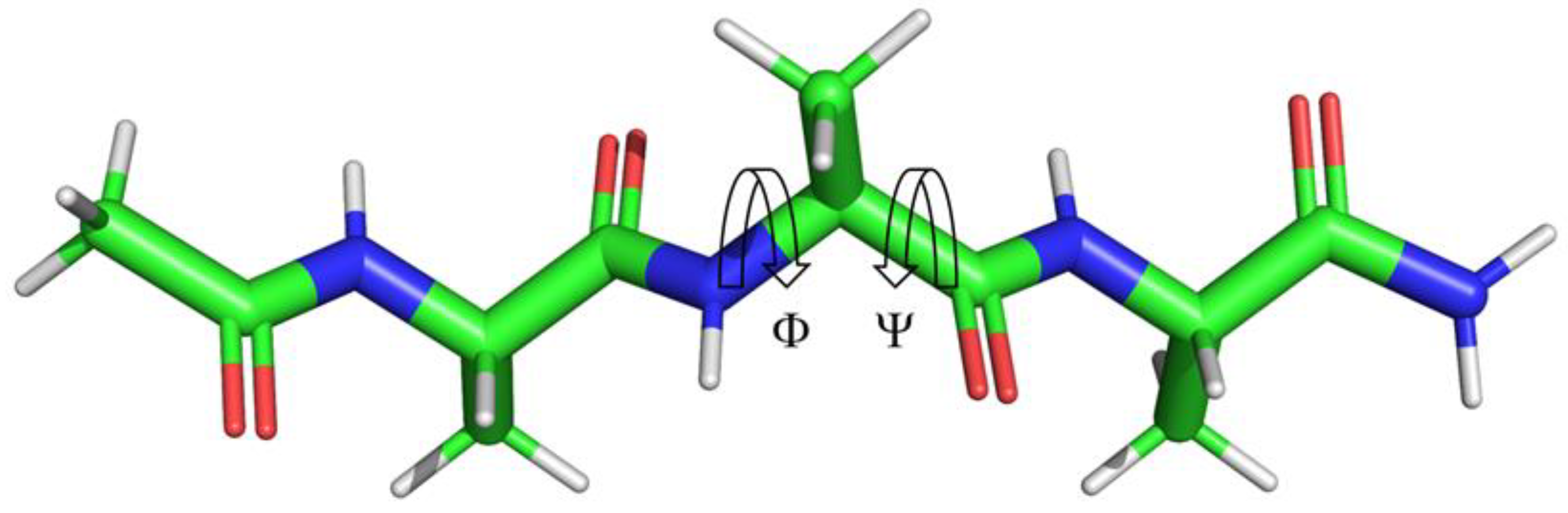
Figure 2.
ϕ,ψ dihedral angles of the central Ala residue of Ac-Ala-Ala-Ala-NH2 peptide in the β, α, αL, and ε regions with representative conformations. Atoms are color coded according to type. C, green; O, red; N, blue; and H, white. Black contour lines represent 98% of the sampled population, brown contour lines represent 99.8%.
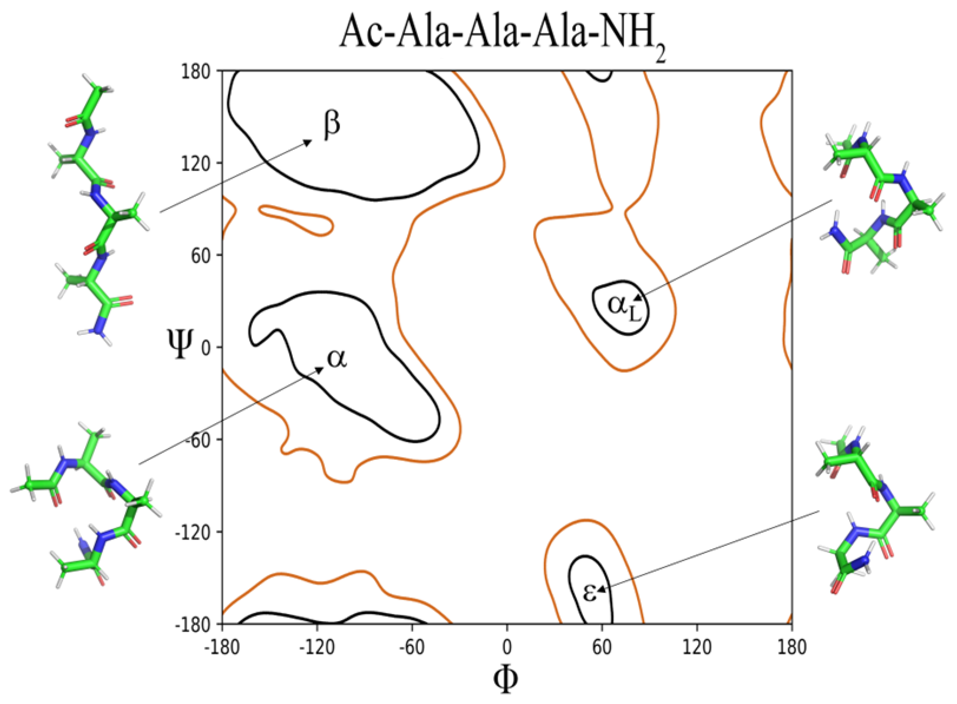
Figure 3.
β, α, αL , and ε conformations of Ac-Ala-Ala-Ala-NH2 demonstrating the changes in backbone(top) and side chain (bottom) of SASA as a function of conformation. SASA is shown as a meshed surface and color coded according to the underlying atom type. C, green; O, red; N, blue; and H, white.
Figure 3.
β, α, αL , and ε conformations of Ac-Ala-Ala-Ala-NH2 demonstrating the changes in backbone(top) and side chain (bottom) of SASA as a function of conformation. SASA is shown as a meshed surface and color coded according to the underlying atom type. C, green; O, red; N, blue; and H, white.
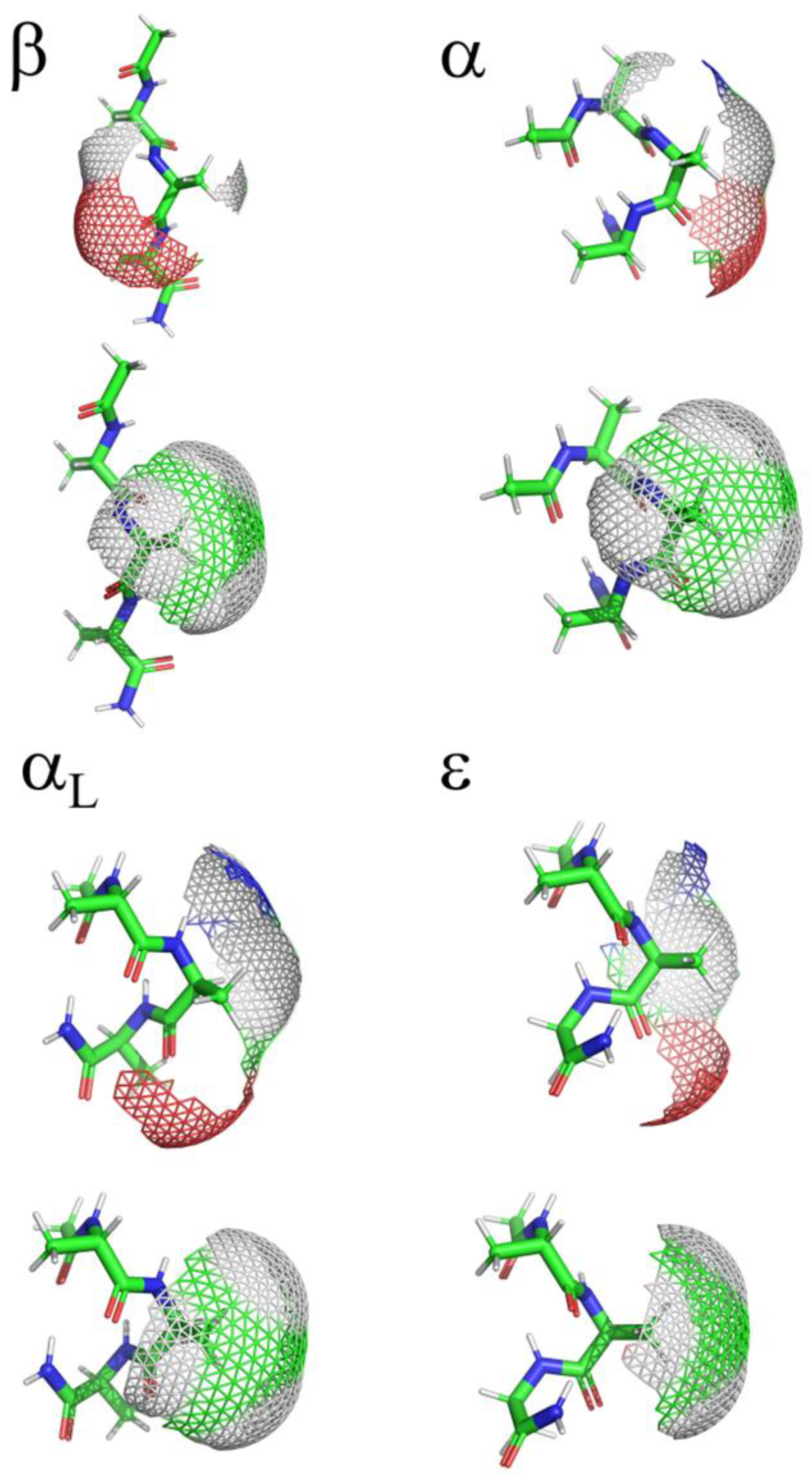
Figure 4.
Two-dimensional histograms demonstrating the log10-scaled probabilities (ρ) of the sampled ϕ,ψ space for the Gly, Ala, Leu, and Ile residues within the Ac-Ala-Xaa-Ala-NH2 peptides demonstrating the effects of side chain size (Gly, Ala, and Leu) and steric properties (Leu and Ile) on ϕ,y space sampling. Black contour lines represent 98% of the sampled population, brown contour lines represent 99.8%.
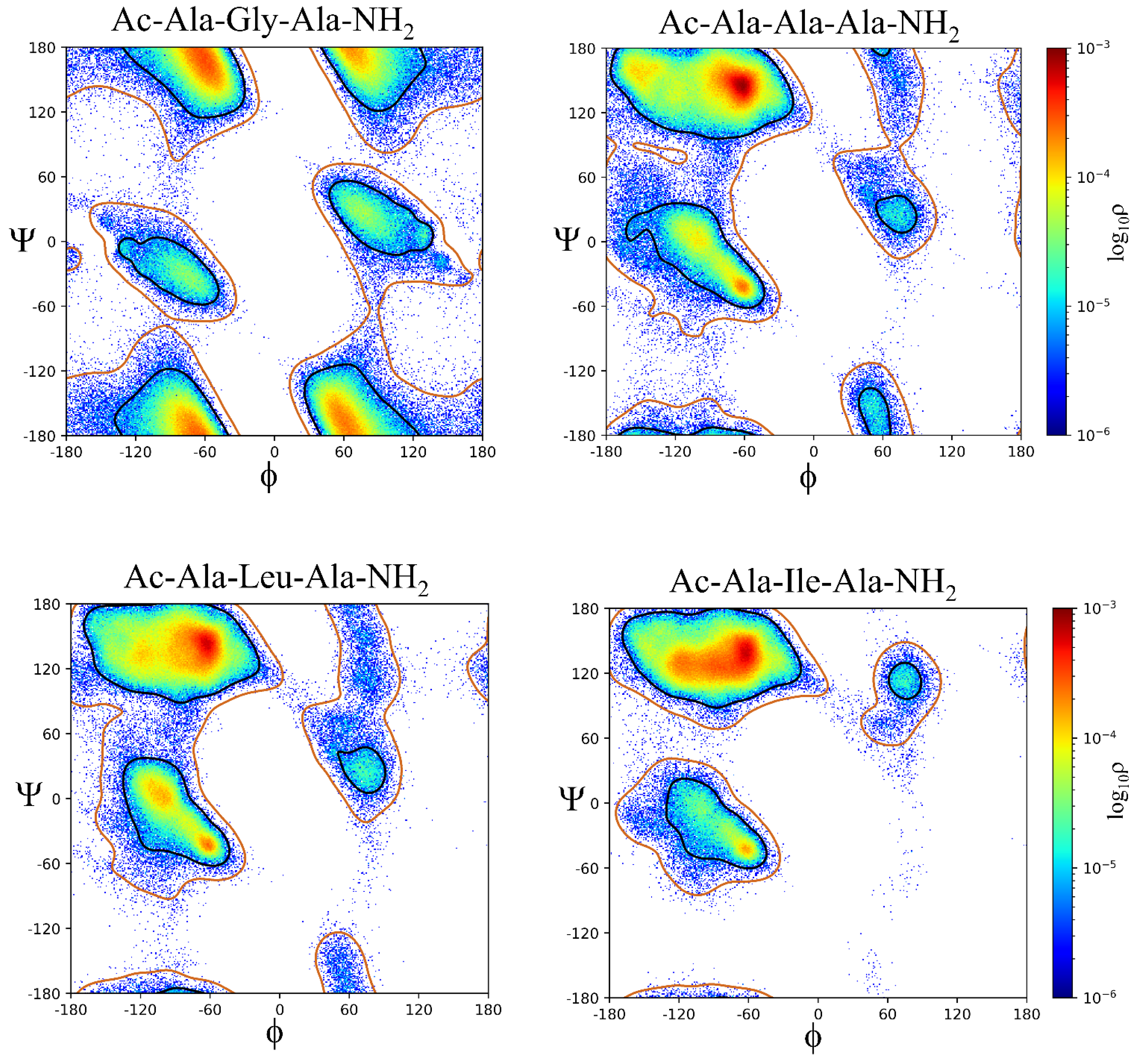
Figure 5.
Two-dimensional histograms demonstrating the log10-scaled probabilities (ρ) of the sampled ϕ,ψ space for the His:ND1, His:NE2, and His+ residues within the Ac-Ala-Xaa-Ala-NH2 peptides demonstrating the effects of side chain protonation state and charge on ϕ,y space sampling. Black contour lines represent 98% of the sampled population, brown contour lines represent 99.8%.
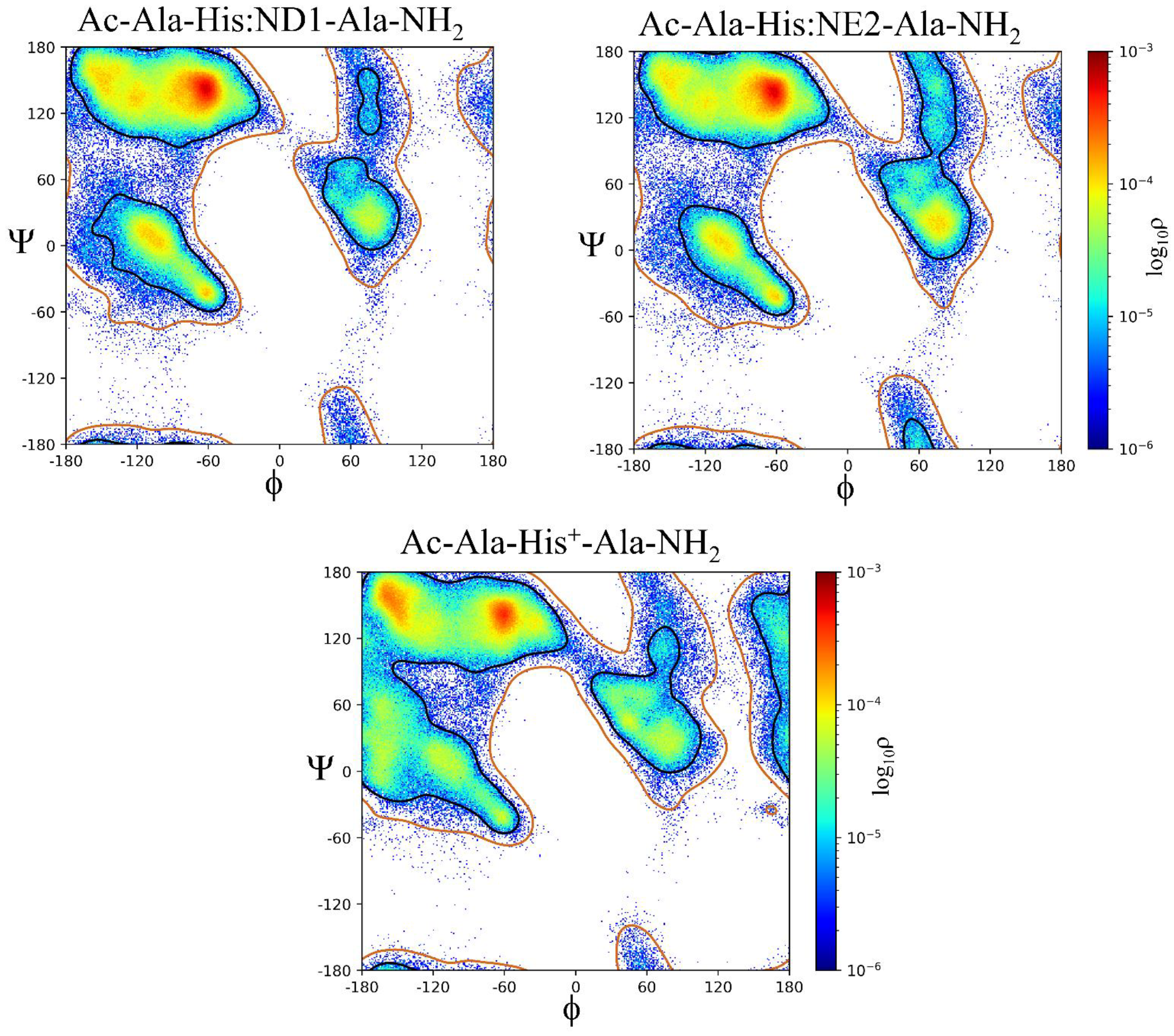
Figure 6.
Two-dimensional histograms demonstrating the log10-scaled probabilities (ρ) of the sampled ϕ,ψ space for the Asp, Asp:H, LysN, and Lys residues within the Ac-Ala-Xaa-Ala-NH2 peptides demonstrating the effects of side chain protonation state and charge on ϕ,y space sampling. Black contour lines represent 98% of the sampled population, brown contour lines represent 99.8%.
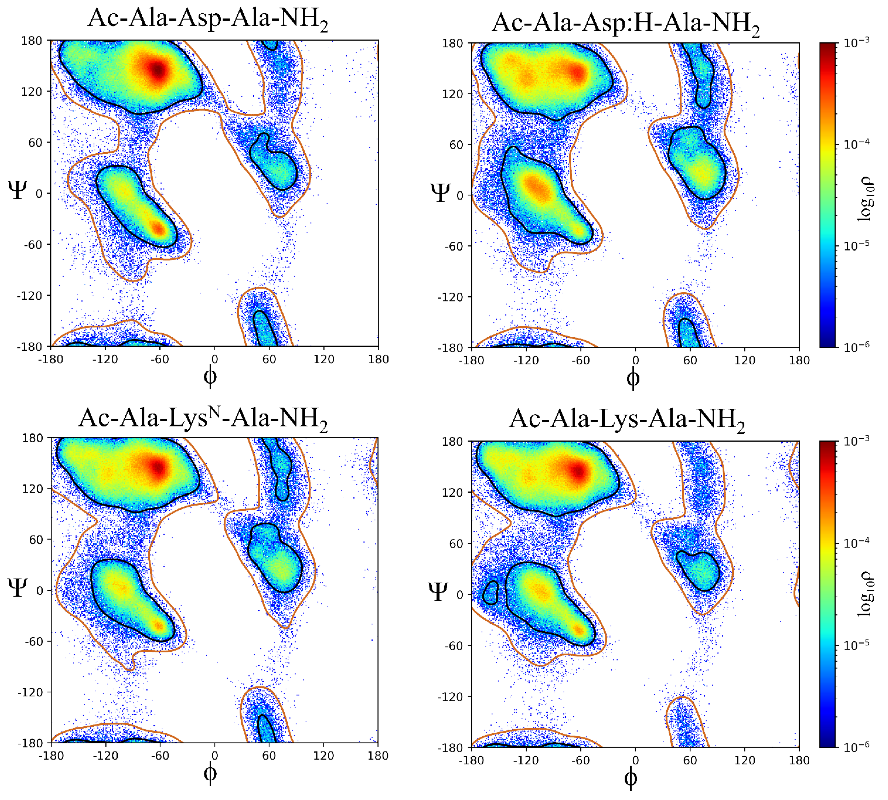
Figure 7.
Two-dimensional histograms demonstrating the log10-scaled probabilities (ρ) of the sampled ϕ,ψ space for the Pro:cis and Pro:trans residues within the Ac-Ala-Xaa-Ala-NH2 peptides demonstrating the effects of the ω dihedral angle between n-1 Ala and Pro with the n-1 residue’s carbonyl oxygen being either cis or trans in its relationship to the Cα of the central Pro on ϕ,y space sampling. Black contour lines represent 98% of the sampled population, brown contour lines represent 99.8%.
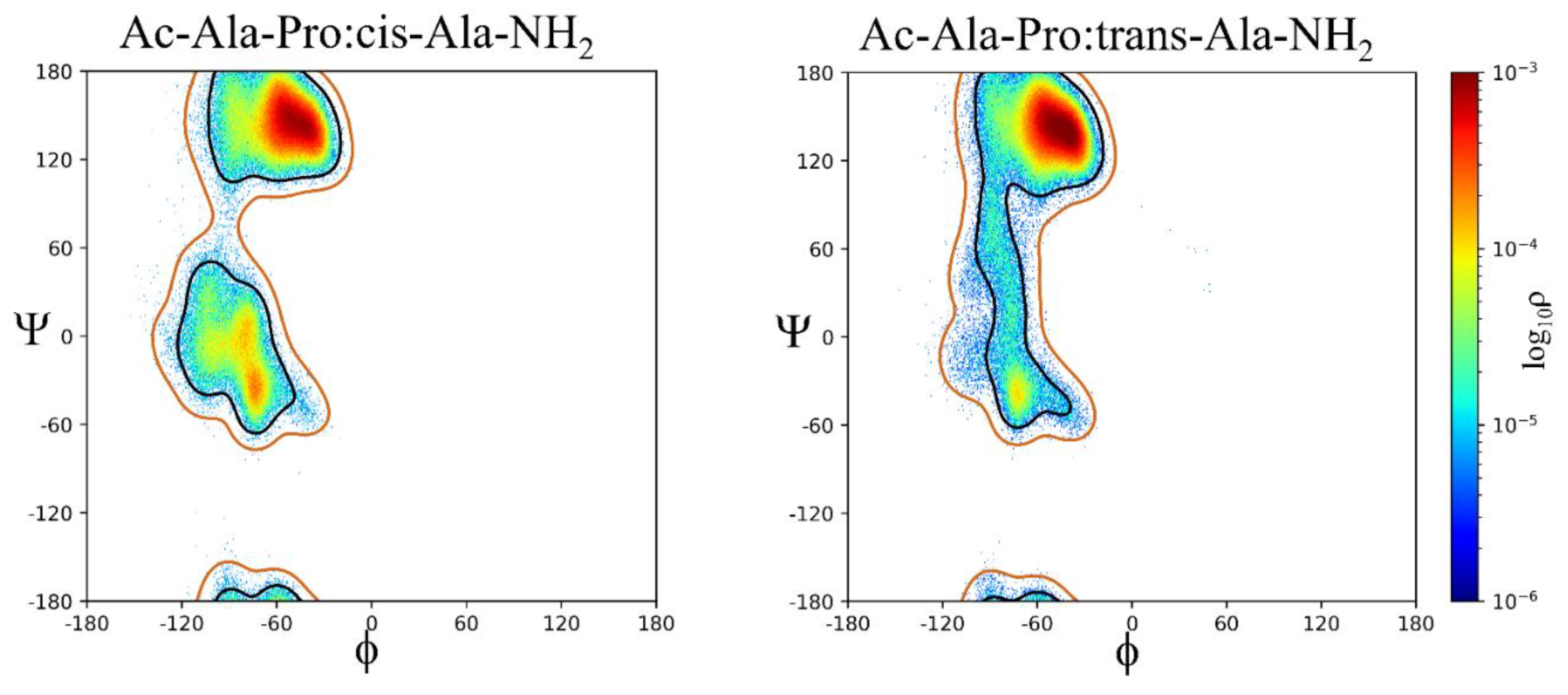
Table 1.
The probability () the Xaa residue within the Ace-Ala-Xaa-Ala-NH2 peptides being within the β, α, αL, ε, or contiguous regions of ϕ,ψ space as assigned by density clustering.a
Table 1.
The probability () the Xaa residue within the Ace-Ala-Xaa-Ala-NH2 peptides being within the β, α, αL, ε, or contiguous regions of ϕ,ψ space as assigned by density clustering.a
| ..Ac-Ala-Xaa-Ala-NH2 | β | α | αL | ε | Cont. |
|---|---|---|---|---|---|
| ρ | ρ | ρ | ρ | r | |
| Gly | 0.4917 | 0.0430 | 0.0586 | 0.3596 | 0.0471 |
| Ala | 0.7636 | 0.1743 | 0.0104 | 0.0112 | 0.0405 |
| Val | 0.9086 | 0.0649 | 0.0103 | N/S | 0.0162 |
| Leu | 0.7395 | 0.2105 | 0.0148 | N/S | 0.0352 |
| Ile | 0.8868 | 0.0878 | 0.0094 | N/S | 0.0160 |
| Met | 0.7308 | 0.1987 | 0.0262 | N/S | 0.0443 |
| His:ND1 | 0.7088 | 0.1740 | 0.0672 | 0.0035 | 0.0465 |
| His:NE2 | 0.6600 | 0.1514 | 0.1219 | 0.0337 | 0.0330 |
| Phe | 0.8160 | 0.1096 | 0.0252 | 0.0094 | 0.0397 |
| Tyr | 0.7850 | 0.1441 | 0.0260 | 0.0067 | 0.0382 |
| Trp | 0.8425 | 0.1199 | 0.0057 | N/S | 0.0320 |
| Ser | 0.7517 | 0.1419 | 0.0320 | 0.0212 | 0.0533 |
| Thr | 0.8407 | 0.1198 | 0.0101 | N/S | 0.0294 |
| Cys:H | 0.7795 | 0.1359 | 0.0445 | N/S | 0.0402 |
| Asn | 0.6309 | 0.2149 | 0.1002 | 0.0248 | 0.0293 |
| Gln | 0.6964 | 0.2296 | 0.0338 | N/S | 0.0402 |
| Arg:NE | 0.7806 | 0.1493 | 0.0291 | N/S | 0.0410 |
| Arg:NH | 0.7415 | 0.1953 | 0.0242 | N/S | 0.0389 |
| Asp:H | 0.6281 | 0.2422 | 0.0806 | 0.0166 | 0.0325 |
| Glu:H | 0.7355 | 0.1981 | 0.0305 | N/S | 0.0359 |
| LysN | 0.7304 | 0.1751 | 0.0478 | 0.0056 | 0.0410 |
| Arg | 0.7781 | 0.1705 | 0.0147 | N/S | 0.0367 |
| His+ | 0.5942 | 0.2020 | 0.1073 | N/S | 0.0964 |
| Lys | 0.7530 | 0.1892 | 0.0180 | N/S | 0.0399 |
| Asp | 0.7675 | 0.1728 | 0.0209 | 0.0068 | 0.0320 |
| Glu | 0.8106 | 0.1506 | 0.0110 | N/S | 0.0278 |
| Cys- | 0.7757 | 0.2134 | N/S | N/S | 0.0109 |
| Tyr- | 0.8201 | 0.1228 | 0.0197 | N/S | 0.0374 |
| Cys-Cys | 0.7406 | 0.1690 | 0.0449 | N/S | 0.0455 |
| Pro:cis | 0.7859 | 0.2104 | N/S | N/S | 0.0037 |
| Pro:trans | 0.9204 | 0.0328 | N/S | N/S | 0.0469 |
a N/S: not sampled region secondary to low population density (<1000 conformations within 10°).
Table 2.
The solvent accessible surface area (SASA) for the whole Xaa residue of Ac-Ala-Xaa-Ala-NH2 as a function of β, α, αL, ε, and contiguous regions of ϕ,ψ space assigned by density clustering.a.
Table 2.
The solvent accessible surface area (SASA) for the whole Xaa residue of Ac-Ala-Xaa-Ala-NH2 as a function of β, α, αL, ε, and contiguous regions of ϕ,ψ space assigned by density clustering.a.
| Ac-Ala-Xaa-Ala-NH2 | All | β | α | αL | ε | Cont. |
|---|---|---|---|---|---|---|
| SASA/nm2 | SASA/nm2 | SASA/nm2 | SASA/nm2 | SASA/nm2 | SASA/nm2 | |
| Gly | 0.788 ± 0.065 | 0.773 ± 0.049 | 0.899 ± 0.047 | 0.895 ± 0.050 | 0.776 ± 0.056 | 0.799 ± 0.083 |
| Ala | 1.093 ± 0.075 | 1.068 ± 0.0059 | 1.188 ± 0.053 | 1.182 ± 0.058 | 1.105 ± 0.058 | 1.111 ± 0.070 |
| Val | 1.523 ± 0.077 | 1.514 ± 0.070 | 1.643 ± 0.061 | 1.516 ± 0.060 | N/S | 1.585 ± 0.087 |
| Leu | 1.857 ± 0.087 | 1.829 ± 0.075 | 1.946 ± 0.060 | 1.940 ± 0.077 | N/S | 1.861 ± 0.090 |
| Ile | 1.749 ± 0.084 | 1.736 ± 0.075 | 1.873 ± 0.069 | 1.727 ± 0.072 | N/S | 1.790 ± 0.084 |
| Met | 1.895 ± 0.117 | 1.864 ± 0.108 | 1.990 ± 0.087 | 2.006 ± 0.096 | N/S | 1.913 ± 0.107 |
| His:ND1 | 1.898 ± 0.100 | 1.864 ± 0.086 | 1.992 ± 0.071 | 2.003 ± 0.075 | 1.890 ± 0.069 | 1.901 ± 0.096 |
| His:NE2 | 1.902 ± 0.101 | 1.867 ± 0.087 | 1.973 ± 0.087 | 2.003 ± 0.079 | 1.887 ± 0.071 | 1.914 ± 0.099 |
| Phe | 2.116 ± 0.099 | 2.097 ± 0.087 | 2.225 ± 0.090 | 2.240 ± 0.086 | 2.094 ± 0.070 | 2.140 ± 0.105 |
| Tyr | 2.258 ± 0.101 | 2.233 ± 0.087 | 2.368 ± 0.087 | 2.384 ± 0.083 | 2.243 ± 0.069 | 2.284 ± 0.102 |
| Trp | 2.513 ± 0.108 | 2.491 ± 0.093 | 2.655 ± 0.099 | 2.486 ± 0.069 | N/S | 2.555 ± 0.108 |
| Ser | 1.209 ± 0.075 | 1.187 ± 0.063 | 1.298 ± 0.055 | 1.299 ± 0.062 | 1.211 ± 0.060 | 1.224 ± 0.074 |
| Thr | 1.415 ± 0.081 | 1.397 ± 0.068 | 1.532 ± 0.059 | 1.401 ± 0.061 | N/S | 1.454 ± 0.088 |
| Cys:H | 1.360 ± 0.080 | 1.338 ± 0.067 | 1.456 ± 0.062 | 1.445 ± 0.072 | N/S | 1.370 ± 0.081 |
| Asn | 1.584 ± 0.085 | 1.549 ± 0.072 | 1.654 ± 0.063 | 1.656 ± 0.068 | 1.551 ± 0.064 | 1.600 ± 0.084 |
| Gln | 1.800 ± 0.105 | 1.767 ± 0.095 | 1.884 ± 0.076 | 1.902 ± 0.089 | N/S | 1.808 ± 0.106 |
| Arg:NE | 2.419 ± 0.128 | 2.392 ± 0.120 | 2.523 ± 0.102 | 2.552 ± 0.100 | N/S | 2.449 ± 0.125 |
| Arg:NH | 2.421 ± 0.124 | 2.394 ± 0.116 | 2.508 ± 0.104 | 2.524 ± 0.102 | N/S | 2.434 ± 0.120 |
| Asp:H | 1.516 ± 0.090 | 1.476 ± 0.075 | 1.590 ± 0.060 | 1.603 ± 0.067 | 1.496 ± 0.068 | 1.537 ± 0.082 |
| Glu:H | 1.810 ± 0.092 | 1.786 ± 0.083 | 1.888 ± 0.077 | 1.890 ± 0.080 | N/S | 1.820 ± 0.092 |
| LysN | 2.092 ± 0.112 | 2.065 ± 0.103 | 2.182 ± 0.092 | 2.194 ± 0.091 | 2.085 ± 0.091 | 2.116 ± 0.107 |
| Arg | 2.409 ± 0.125 | 2.386 ± 0.119 | 2.503 ± 0.105 | 2.499 ± 0.112 | N/S | 2.425 ± 0.123 |
| His+ | 1.879 ± 0.108 | 1.845 ± 0.092 | 1.928 ± 0.106 | 1.985 ± 0.086 | N/S | 1.872 ± 0.111 |
| Lys | 2.127 ± 0.106 | 2.100 ± 0.096 | 2.217 ± 0.087 | 2.232 ± 0.090 | N/S | 2.144 ± 0.104 |
| Asp | 1.480 ± 0.079 | 1.455 ± 0.063 | 1.574 ± 0.065 | 1.575 ± 0.057 | 1.477 ± 0.055 | 1.502 ± 0.079 |
| Glu | 1.774 ± 0.084 | 1.753 ± 0.072 | 1.871 ± 0.069 | 1.878 ± 0.064 | N/S | 1.807 ± 0.084 |
| Cys- | 1.375 ± 0.082 | 1.350 ± 0.065 | 1.469 ± 0.067 | N/S | N/S | 1.379 ± 0.083 |
| Tyr- | 2.205 ± 0.109 | 2.181 ± 0.097 | 2.320 ± 0.094 | 2.358 ± 0.065 | N/S | 2.255 ± 0.093 |
| Cys-Cys | 0.753 ± 0.141 | 0.735 ± 0.134 | 0.796 ± 0.145 | 0.819 ± 0.148 | N/S | 0.761 ± 0.135 |
| Pro:cis | 1.476 ± 0.060 | 1.461 ± 0.055 | 1.533 ± 0.040 | N/S | N/S | 1.482 ± 0.090 |
| Pro:trans | 1.415 ± 0.056 | 1.407 ± 0.047 | 1.534 ± 0.043 | N/S | N/S | 1.489 ± 0.074 |
a N/S: not sampled region secondary to low population density (<1000 conformations within 10°).
Disclaimer/Publisher’s Note: The statements, opinions and data contained in all publications are solely those of the individual author(s) and contributor(s) and not of MDPI and/or the editor(s). MDPI and/or the editor(s) disclaim responsibility for any injury to people or property resulting from any ideas, methods, instructions or products referred to in the content. |
© 2024 by the authors. Licensee MDPI, Basel, Switzerland. This article is an open access article distributed under the terms and conditions of the Creative Commons Attribution (CC BY) license (http://creativecommons.org/licenses/by/4.0/).
Copyright: This open access article is published under a Creative Commons CC BY 4.0 license, which permit the free download, distribution, and reuse, provided that the author and preprint are cited in any reuse.


