Submitted:
29 July 2024
Posted:
01 August 2024
You are already at the latest version
Abstract
This study presents a detailed investigation of the application of superquadrics in small-angle scattering (SAS), a technique essential in materials science, biology, and physics for investigating structural properties at the nanoscale and microscale. Superquadrics, a family of geometric shapes known for their versatility in representing a wide range of forms, are employed to model complex structures in SAS studies. We examine the parametric nature of superquadrics and their ability to efficiently describe shapes from simple balls to intricate star-like forms. We demonstrate the application of superquadrics through a rigorous analysis of SAS simulated data, including scattering intensity patterns and pair-distance distribution functions. This allows us to reveal insights into key structural characteristics of various materials, such as the size and shape. We also demonstrate the efficacy of superquadrics in accurately modeling experimental small-angle X-ray scattering data from a chimeric protein complex, showcasing their potential in biological systems analysis. The findings offer a robust framework for future research and application in diverse fields, including materials science, nanotechnology, and bioengineering.
Keywords:
small-angle scattering
; superquadrics
; complex systems.
1. Introduction
Superquadrics, a versatile family of geometric shapes defined by a set of parametric equations, have emerged as important tools in a wide range of fields. Their applications span from computer graphics [1] and robotics [2] to the structural modeling of nano and microstructures [3]. The adaptability of superquadrics, which can represent structures, ranging from simple balls to complex star-like forms, is underpinned by their geometric flexibility [4] and computational efficiency [5]. This makes them particularly useful in fields such as materials science, nanotechnology, and bioengineering, where a precise characterization of geometric properties is crucial for exploiting the shape-dependent properties of particles at the nano and microscale.
Small-angle scattering (SAS; [6,7,8]) of X-rays (SAXS) or neutrons (SANS) is a non-destructive analytical technique widely used in material science [9,10,11], biology [12,13,14,15,16,17,18], chemical physics [19,20,21,22,23], cellular automata [24,25] or in studying the geometrical properties of fractal systems [26,27,28,29,30]. It measures the intensity of scattered radiation at small angles and is commonly used in studying the size, shape, and distribution of particles at the nano and microscale, owing to its sensitivity to variations in scattering length density caused by inhomogeneities within a sample.
In the specific context of SAS analysis, superquadrics address a critical challenge: the modeling of structures that deviate from idealized geometries. Traditional SAS models are effective for well-defined shapes like spheres, cubes, and ellipsoids [31], but they struggle with structures that exhibit transitional or complex features. In the latter case additional approaches, often complicated, are used, including exploiting specific properties such as exact self-similarity [26] or involving molecular dynamics simulations [32]. This limitation to simple shapes is particularly acute in the study of biological macromolecules and nanomaterials, where diverse shapes often defy simple geometric categorization. Superquadrics offer a solution by providing a parametric framework capable of describing a broad spectrum of shapes, including those that transition between traditional geometric forms.
This adaptability of superquadrics is crucial for analyzing scattering data from materials with varied morphologies that can be modeled with precise geometric structures, such as those with rounded or sharp edges and clear symmetrical properties [33]. When modeling organic and more complex structures, then generalizations of superquadrics, to supershapes [34] and rational supershapes [35] can be further considered. However, direct mathematical equivalence between specific supershapes and superquadrics isn’t straightforward due to their different foundational equations. In the former case the corresponding equation introduces additional parameters and does not map directly onto the equation of superquadrics. Still, by adjusting the supershapes parameters, one can achieve visually similar results to those of superquadrics, especially for certain symmetries and aspect ratios.
Therefore, in this study we explore the integration of superquadrics within SAS analysis, focusing on their effectiveness in scenarios where the simplicity and clarity of geometric forms are essential for the accurate interpretation of SAS data. The role and impact of the parameters appearing in the superquadrics equation are investigated in detail. To this aim, superquadrics are treated as randomly oriented and distributed inhomogeneities within a matrix, allowing for an efficient description and analysis of SAS data, including scattering intensity patterns and pair-distance distribution functions. We identify six general classes of superquadric shapes, each characterized by specific parameters, and conduct a rigorous analysis to unveil key structural characteristics such as size and shape. Our findings reveal that scattering intensities and pair-distance distribution functions possess distinctive features that can differentiate between various superquadric classes.
Furthermore, we demonstrate the practical application of this approach by modeling experimental SAXS data from a chimeric protein complex [36]. This application highlights the potential of superquadrics in biological system analysis, particularly in elucidating the contribution of different protein domains to the overall scattering intensity. The study thus presents superquadrics not only as a theoretical advancement but also as a practical tool for enhancing the understanding of complex structures with SAS analysis.
2. Theoretical Background
2.1. Superquadrics
The general form of the superquadric is given by the following parametric equations [37]:
In these equations, a, b, and c represent the semi-dimensions of the superquadric along the x, y, and z axes, respectively. These dimensions define the scale of the superquadric in each of the principal directions, thereby determining its overall size and proportion. The angular parameters and vary over the ranges and , respectively, sweeping the entire surface of the superquadric. The sign function, defined as:
is used to handle the signs of the cosine and sine terms, which is crucial for accurately representing the shape’s geometry, especially when dealing with negative exponents. The use of the sign function ensures that the superquadric shape is correctly formed in all quadrants of the coordinate system, maintaining the correct orientation and symmetry.
The exponents and in Eq. (1) are shape parameters that control the ’squareness’ or ’roundness’ of the superquadric. By adjusting these parameters, a wide variety of shapes can be generated (see Figure 1), ranging from spherical forms (when and are close to 1) to box-like shapes with sharp edges and flat faces (as and increase). This flexibility makes superquadrics very useful in various applications, particularly in structural modeling, where they are employed to represent complex shapes and surfaces efficiently [38,39,40,41].
2.2. Small-Angle Scattering
The fundamental principle of SAS lies in the analysis of the scattering intensity , i. e. the elastic cross section per unit solid angle, as a function of the magnitude of the scattering vector, defined as , where is the wavelength of the incident radiation, and is the scattering angle [13,42].
In the case of a single particle in a fixed orientation in vacuum, let us consider first the electron density that gives the number of electrons per unit volume a the position r. Then the scattering amplitude of the particle can be expressed as the Fourier transform of the electron-density distribution , as [43]:
Here, V is the irradiated volume, and is the volume element that contains electrons at position r.
Then, the corresponding intensity is given by the product of the amplitude and its complex conjugate [44], i.e.:
which is expressed in terms of the convolution square:
In the realm of SAS analysis, certain simple geometric shapes allow for the derivation of analytic expressions for their scattering amplitudes. These expressions are invaluable for interpreting scattering data and understanding the underlying structural characteristics of the material under study. A quintessential example is the scattering amplitude of a sphere. For a homogeneous sphere of radius R, the scattering amplitude can be analytically expressed as a function of the scattering vector q. This is given by the well-known formula [45]:
For a collection of statistically isotropic particles, without long-range order, embedded in a homogeneous matrix with electron density , the electron density is replaced by . Then, by taking into account that the convolution square of this difference density is related to the pair-distance distribution function [46] by , the scattering intensity of the whole collection can be written in terms of the as [43]:
Thus, the is a critical concept in SAS analysis, particularly when examining collections of points. It represents a histogram of the frequency of distances between all pairs of points within the scattering volume. Essentially, describes how the density of scattering material varies as a function of distance within the particle. This function is particularly insightful as it provides a real-space interpretation of the scattering data, which is inherently collected in reciprocal space. In the case of a sphere of radius R, has an analytic expression, as given by [47]:
One of the primary properties of the is that it peaks at distances corresponding to the most prevalent inter-particle separations within the sample. For instance, in a system of uniform spherical particles, would exhibit a peak corresponding to the radius of the spheres [43]. The function diminishes to zero for distances larger than the maximum dimension of the scattering entity, denoted as D. This characteristic of the provides important information about the overall size and shape of the particles or structures under study. Moreover, the area under the curve is proportional to the square of the volume of the scattering entity, offering insights into the particle’s size and density.
In particular, the radius of gyration (), which is a measure of the distribution of the components of the scattering particle around its center of mass, is the main quantity used to infer its size and shape. Moreover, when not the whole curve is available from experimental data, can be determined form the low-angle part of the scattering data, often using the Guinier approximation [48], which states that:
3. Results and Discussion
Here, the parameters Å are held constant across all shapes. This is because variations in these parameters, while affecting the size of the superquadrics, do not significantly alter the fundamental structural properties under investigation. Basically, they elongate the shapes along one or two spatial dimensions. This gives rise to certain well-established regions where the scattering intensity exhibits a decay proportional to or (depending on the relative values of a, b and c) [11,31].
3.1. Models
The shape parameters and control the squareness of the superquadric in the respective directions. The most common shapes of a superquadric can be classified based on the values of and :
- Ellipsoid: When both and equal 1, the superquadric takes on the form of an ellipsoid. This shape is characterized by its uniform curvature and is commonly used to model objects with spherical or ellipsoidal characteristics.
- Octahedron: As and increase beyond 1, the superquadric becomes more box-like with sharper edges. This configuration resembles an octahedron and is suitable for representing objects with angular features.
- Elliptic bicone: When is greater than 1 and equals 1, the superquadric exhibits the appearance of two cones sharing a common elliptical base. This shape is well-suited for modeling objects with conical attributes
- Elliptic pillow: Conversely, when equals 1 and is greater than 1, the superquadric takes on a form reminiscent of four half-regions with common elliptical bases. This configuration is useful for objects that possess pillow-like structures.
- Near-cube: When both and are between 0 and 1, the superquadric approaches a cube-like shape. It is an ideal choice for representing objects that are nearly cubic in nature.
- Star: Finally, by setting both and greater than 2, the superquadric exhibits concave features resembling a star-like shape. This configuration is valuable for modeling objects with intricate concavities.
Note that in the literature, these classes with and are also known generically as superellipsoids [49]. Structures corresponding to certain values of and/or are given particular names, e.g. supereggs, when or superspheres, when [49].
The visual representations in Figure 1 showcase examples of superquadrics from each of these classes. These variations in shape parameters highlight the adaptability and versatility of superquadric models in geometric modeling, allowing researchers and designers to accurately capture a wide range of structural and geometrical properties in their models [38,39].
It’s worth noting that while the classification of superquadrics into these distinct classes based on shape parameters and provides a comprehensive framework for understanding their geometrical properties, it does not encompass all possible superquadric structures. There exist configurations beyond these classes, but they tend to be more exotic and less commonly used in geometrical modeling. These "exotic" superquadrics may have highly specialized shapes or intricate combinations of parameters that are less practical for general-purpose modeling. Nevertheless, the established classes we discuss here serve as a robust foundation for modeling a wide range of objects encountered in various fields, offering a balance between flexibility and practicality in geometrical modeling applications.
3.2. Pair-distance distribution functions and scattering intensities
The pair-distance distribution function is evaluated by randomly generating 50000 particles within each shape. For globular shapes, this number of particles is generally sufficient to provide accurate scattering data over an extended q-range, which is useful for data analysis [16,17,20]. The scattering intensity is then calculated by using Eq. (7), for various superquadric shapes from each class depicted in Figure 1. For each combination of , ten trials are conducted.
To ensure the validity of the approach employed, Figure 2(a) includes the given by Eq. (8), with . The results show an excellent agreement between the theoretical and the simulated one (green continuous curve).
The simulated profiles, as illustrated in Figure 2(a), predominantly exhibit a bell-shaped behavior. This characteristic suggests a high degree of symmetry in relation to the center of mass for all the shapes considered. Nonetheless, distinct features in are observed for each superquadric class.
Ellipsoids and near-cubes, known for their uniform curvature, exhibit smooth curves. In contrast, shapes with more angular geometries, such as octahedrons, display sharper peaks in their functions. The peaks are associated with the most common distances within the shape. Thus, octahedron pattern suggests a higher prevalence of certain inter-particle distances, uniquely characteristic of these shapes, and which arise due the the lower symmetry as compared to spheres or near-cubes. Moreover, the star shape, marked by its concavities, reveals a more complex pattern. Here, the maxima are noticeably shifted towards smaller values, and the frequency of the most common distances is significantly higher compared to other curves. This observation is attributed to the numerous distances within the branches of the star, underscoring the complexity and nuanced spatial arrangement inherent to this shape. In general, the value at which these peaks occur, tends to be smaller with decreasing the symmetry.
The scattering intensities, obtained from the Fourier transform of as per Eq. (7), shed light on the size and shape of the scattering entities. Notably, certain features, such as the radius of gyration and the self-similarity of the systems, are more readily discerned in reciprocal space [30,50]. This aspect becomes crucial, particularly when the experimental data is incomplete or lacks the necessary range for a thorough analysis of from . The accuracy of the Fourier transformation used is further verified against the analytical expression of the sphere’s scattering amplitude (black dashed line), given by: Eq. (6).
Typically, the scattering curves exhibit a Guinier region (for ) followed by a Porod region (for ), where the scattering intensity, characterized by alternating maxima and minima, decays according to a power-law proportional to [51]. However, in physical experiments, the scattering curves are often smoothed due to various factors, such as finite instrument resolution or the presence of non-ideally monodisperse systems [52]. In this study, we replicate these effects by applying locally weighted scatterplot smoothing (LOWESS [53]; with a span of 0.12) to the scattering intensities, facilitating a more accurate exploration of the trends in scattering intensity.
Distinct intensity patterns are observed across different superquadric classes, as illustrated in Figure 2(b). For simpler shapes like ellipsoids and near-cubes, show a more predictable and smoother decay with increasing q. For some particular parameter values of the superquadrics, a form factor that describes the transition between these two shapes is available [33]. In contrast, complex shapes such as star-shaped superquadrics exhibit more pronounced fluctuations, reflective of their intricate internal structures. Additionally, the Guinier region for the star shape is notably elongated compared to other shapes. This phenomenon can be attributed to the fact that, despite having similar overall dimensions, a significant portion of the points generated for the star shape (as shown in Figure 1) are concentrated in a much smaller region, while the remainder extend along the branches.
Differences in the scattering patterns are utilized to determine the radii of gyration. To this end, we conduct a Guinier analysis by plotting against , as outlined in Eq.(9) and illustrated in Figure 3. For each dataset, a linear fit is applied for values where . The slopes of these fits () and the corresponding radii of gyration () are detailed in Tab. Table 1. Our findings reveal that the radius of gyration for the star shape is approximately three times smaller than that of the ellipsoid or near-cube, and about twice as small compared to the elliptic bicone or elliptic pillow, in line with the qualitative predictions seen in Figure 2(b).
3.3. Application: Analysis of Small-angle X-ray Scattering Data from a Chimeric Protein complex
To demonstrate the capability of superquadrics in modeling structures at the nano and micro scales, this section focuses on a biological system comprising a ferritin-based fusion protein. SAXS data were collected for a solution containing a 24-meric ferritin-based protein complex, fused with a SMT3 protein tag (a homolog of the human Small Ubiquitin-like Modifier; SUMO), in a medium of 25 mM Tris, 150 mM NaCl, and pH 7.4 [36]. The SAXS data underwent normalization to the intensity of the transmitted beam, followed by radial averaging and subtraction of solvent-blank scattering. The corresponding SAXS data and models were retrieved from the Small Angle Scattering Biological Data Bank (SASBDB [54]), with the specific dataset identified as: SASDTU4.
Figure 4(a) presents the chimeric protein complex of ferritin from Helicobacter pylori, designated with the UniProt [55] ID: 3BVE. This figure highlights the C-terminal region of the protein construct employed in SAXS measurements. The N-terminal region comprises a His-SUMO-tag, corresponding to UniProt ID Q12306, and includes amino acids 3-98 with the mutations R64T and R71E. The protein complex distinctly reveals a star-like configuration, featuring a central core (ferritin) to which several branches (SMT3 tags) are connected. Overlaying this molecular structure is a star-shaped superquadric model (transparent light-blue region), which closely approximates the overall form of the protein complex. However, some extremities of the branches are observed to extend beyond the confines of the superquadric model.
The experimental SAXS curve (represented by black dots) alongside the intensity profile of the star-shaped superquadric (depicted as the green curve) is presented in Figure 4(b). A constant term of has been added to the calculated intensity. This adjustment accounts for the experimental background scattering, as illustrated by the horizontal dark-green dashed line. The results align very well up to a q value of approximately . Beyond this point, it is observable that the simulated curve slightly undershoots the experimental data, despite the high error margins associated with the experimental measurements.
Given that the radius of gyration of the core is about (significantly smaller than that of the entire complex, which is approximately , as indicated by the blue curve in the plot of Eq. (9)), the dominant contribution in this region arise from the shorter distances between particles, primarily within the branches. Consequently, increasing the number of generated points, thereby reducing the distances between them, can enhance the resemblance of their distribution to the actual shape of the branches, especially at the extremities. This adjustment is expected to result in an improved agreement with the SAXS curve at higher q-values.
4. Conclusions
This study explores the applicability of superquadrics in SAS analysis, showcasing their efficacy in modeling diverse structures at the nanoscale and microscale. By harnessing the parametric nature of superquadrics, this investigation delves into their versatility in representing various shapes, ranging from spherical entities to complex star-like formations. The results demonstrate the capability of superquadrics to efficiently describe structural properties within SAS datasets, elucidating insights into size, shape, and distribution of scattering entities.
The pair-distance distribution functions () and the corresponding scattering intensities () derived from different superquadric shapes exhibit distinctive patterns reflective of their geometric attributes. Shapes like ellipsoids and near-cubes manifest smooth curves, while more angular geometries like octahedrons display sharper peaks, signifying distinct inter-particle distances prevalent within these shapes. Furthermore, complex structures such as star-shaped superquadrics unveil intricate patterns, highlighting the nuanced spatial arrangements inherent in these branched configurations. The Guinier analysis of the scattering intensities reveals characteristic radii of gyration () for each superquadric class, offering insights into the distribution of density around the corresponding center of masses.
Additionally, the application of superquadrics in modeling small-angle X-ray scattering (SAXS) data from a chimeric protein complex underscores their potential in accurately approximating complex biological structures. The close agreement between the star-shaped superquadric model and the experimental SAXS data highlights the utility of superquadrics in representing intricate molecular architectures consisting of various protein domains, thus providing a robust framework for structural analysis.
Overall, this study underscores the significance of superquadrics as versatile tools in geometric modeling, offering a comprehensive approach to characterize and analyze structures across various scales and disciplines. The insights gained herein pave the way for future advancements in SAS analysis, facilitating a deeper understanding of structural properties in diverse materials and biological systems. In materials science, this could lead to the development of novel nanostructured materials whose properties are tailored through precise geometric control. Such materials could find applications in areas ranging from photonic crystals and drug delivery systems to novel catalysts and energy storage devices. In bioengineering, the ability to accurately model and analyze the structural properties of biological macromolecules using superquadrics could significantly enhance our understanding of biomolecular interactions and stability. This could lead to breakthroughs in the design of biomimetic materials, tissue engineering, and the development of targeted therapeutic agents.
While this study demonstrates the significant potential of superquadrics in SAS analysis, it is important to acknowledge certain limitations. The current research primarily focuses on idealized superquadric shapes, which, although versatile, may not capture the full complexity of certain real-world nano and microstructures. For instance, materials with irregular surface textures or internal heterogeneities may not be accurately modeled by the smooth and continuous surfaces of superquadrics. Additionally, the assumption of uniform material density within the region delimited by the superquadric may not hold true for all materials, particularly those with graded or layered compositions.
Future research could explore the integration of superquadrics with more complex modeling techniques to better represent materials with non-uniform densities and irregular surfaces. This could include hybrid models that combine superquadrics with fractal or stochastic elements to capture the intricacies of materials like porous polymers, composite nanoparticles, or biological assemblies with non-uniform density distributions. Another promising avenue is the application of superquadrics to the study of soft matter systems like colloidal clusters, where the shapes often deviate significantly from standard geometric forms.
Declarations
The author has no competing interests to declare that are relevant to the content of this article. The manuscript has no associated data.
Data Availability Statement: No Data associated in the manuscript.
References
- Vaskevicius, N.; Birk, A. Revisiting Superquadric Fitting: A Numerically Stable Formulation. IEEE Trans. Pattern Anal. Mach. Intell. 2019, 41, 220–233. [Google Scholar] [CrossRef]
- Vezzani, G.; Pattacini, U.; Natale, L. A grasping approach based on superquadric models. Proc. - IEEE Int. Conf. Robot. Autom, 2017, pp. 1579–1586. [CrossRef]
- Torres-DÃ az, I.; Hendley, R.S.; Mishra, A.; Yeh, A.J.; Bevan, M.A. Hard superellipse phases: particle shape anisotropy & curvature. Soft Matter 2022, 18, 1319–1330. [Google Scholar]
- Burugadda, P.; Likhith Kumar Reddy, S.; Govardhan Kumar, S.; Katakam, G.; Prashanth Kumar, Y. Parametrization of 3D shapes using Superquadrics. Proc. - IEEE Int. Conf. Smart Electron. Commun., 2020, pp. 620–624.
- Wang, S.; Zhang, Q.; Ji, S. GPU-based Parallel Algorithm for Super-Quadric Discrete Element Method and Its Applications for Non-Spherical Granular Flows. Adv. Eng. Softw. 2021, 151, 102931. [Google Scholar] [CrossRef]
- Anitas, E.M. Introduction. In Small-Angle Scattering (Neutrons, X-Rays, Light) from Complex Systems: Fractal and Multifractal Models for Interpretation of Experimental Data; Springer International Publishing: Cham, 2019; pp. 1–7. [Google Scholar] [CrossRef]
- Anitas, E.M. , X-Rays, Light) from Complex Systems: Fractal and Multifractal Models for Interpretation of Experimental Data; Springer International Publishing: Cham, 2019; pp. 33–63. doi:10.1007/978-3-030-26612-7_3.Technique. In Small-Angle Scattering (Neutrons, X-Rays, Light) from Complex Systems: Fractal and Multifractal Models for Interpretation of Experimental Data; Springer International Publishing: Cham, 2019; Springer International Publishing: Cham, 2019; pp. 33–63. [Google Scholar] [CrossRef]
- Hamley, I.W. Small-Angle Scattering: Theory, Instrumentation, Data, and Applications, 1st ed.; Wiley, Hoboken, NJ, USA, 2021.
- Melnichenko, Y.B.; Wignall, G.D. Small-angle neutron scattering in materials science: Recent practical applications. J. Appl. Phys. 2007, 102, 021101. [Google Scholar] [CrossRef]
- Anitas, E.M. Structural Properties of Molecular Sierpinski Triangle Fractals. Nanomaterials 2020, 10. [Google Scholar] [CrossRef]
- Anitas, E.M. Small-Angle Scattering from Fractional Brownian Surfaces. Symmetry 2021, 13. [Google Scholar] [CrossRef]
- Jacques, D.A.; Trewhella, J. Small-angle scattering for structural biologyâExpanding the frontier while avoiding the pitfalls. Protein Sci. 2010, 19, 642–657. [Google Scholar] [CrossRef]
- Svergun, D.I.; Koch, M.H.J. Small-angle scattering studies of biological macromolecules in solution. Rep. Prog. Phys. 2003, 66, 1735. [Google Scholar] [CrossRef]
- Anitas, E.M.; Slyamov, A. Structural characterization of chaos game fractals using small-angle scattering analysis. PLOS ONE 2017, 12, 1–16. [Google Scholar] [CrossRef]
- Anitas, E.M. Small-Angle Scattering and Multifractal Analysis of DNA Sequences. Int. J. Mol. Sci. 2020, 21. [Google Scholar] [CrossRef]
- Anitas, E.M. α-SAS: an integrative approach for structural modeling of biological macromolecules in solution. Acta Crystallogr. D 2022, 78, 1046–1063. [Google Scholar] [CrossRef]
- Anitas, E.M. Fractal Analysis of DNA Sequences Using Frequency Chaos Game Representation and Small-Angle Scattering. Int. J. Mol. Sci. 2022, 23. [Google Scholar] [CrossRef]
- Anitas, E.M. Integrating machine learning with -SAS for enhanced structural analysis in small-angle scattering: applications in biological and artificial macromolecular complexess. Eur. Phys. J. E 2024, 47, 198–206. [Google Scholar] [CrossRef]
- Fritz, G.; Bergmann, A.; Glatter, O. Evaluation of small-angle scattering data of charged particles using the generalized indirect Fourier transformation technique. J. Chem. Phys. 2000, 113, 9733–9740. [Google Scholar] [CrossRef]
- Anitas, E.M. Structural Properties of Janus Particles with Nano- and Mesoscale Anisotropy. Nanomaterials 2020, 10. [Google Scholar] [CrossRef]
- Anitas, E.M. Structural characterization of Janus nanoparticles with tunable geometric and chemical asymmetries by small-angle scattering. Phys. Chem. Chem. Phys. 2020, 22, 536–548. [Google Scholar] [CrossRef]
- Cherny, A.Y.; Anitas, E.M.; Osipov, V.A. Dense random packing with a power-law size distribution: The structure factor, massâradius relation, and pair distribution function. J. Chem. Phys. 2023, 158, 044114. [Google Scholar] [CrossRef]
- Cherny, A.Y.; Anitas, E.M.; Vladimirov, A.A.; Osipov, V.A. Dense random packing of disks with a power-law size distribution in thermodynamic limit. J. Chem. Phys. 2024, 160, 024107. [Google Scholar] [CrossRef]
- Anitas, E.M.; Slyamov, A.M. Emergence of Surface Fractals in Cellular Automata. Ann. Phys. 2018, 530, 1800187. [Google Scholar] [CrossRef]
- Anitas, E.M.; Slyamov, A. Structural Properties of Additive Nano/Microcellular Automata. Ann. Phys. 2018, 530, 1800004. [Google Scholar] [CrossRef]
- Anitas, E.M. Small-angle scattering from fat fractals. Eur. Phys. J. B 2014, 87. [Google Scholar] [CrossRef]
- Anitas, E.M. Fractals: Definitions and Generation Methods. In Small-Angle Scattering (Neutrons, X-Rays, Light) from Complex Systems: Fractal and Multifractal Models for Interpretation of Experimental Data; Springer International Publishing: Cham, 2019; pp. 9–31. [Google Scholar] [CrossRef]
- Anitas, E.M. Small-Angle Scattering from Fractals. In Small-Angle Scattering (Neutrons, X-Rays, Light) from Complex Systems: Fractal and Multifractal Models for Interpretation of Experimental Data; Springer International Publishing: Cham, 2019; pp. 65–111. [Google Scholar] [CrossRef]
- Anitas, E.M. Conclusions and Outlook. In Small-Angle Scattering (Neutrons, X-Rays, Light) from Complex Systems: Fractal and Multifractal Models for Interpretation of Experimental Data; Springer International Publishing: Cham, 2019; pp. 113–116. [Google Scholar] [CrossRef]
- Anitas, E.M. Small-Angle Scattering from Fractals: Differentiating between Various Types of Structures. Symmetry 2020, 12. [Google Scholar] [CrossRef]
- Pedersen, J.S. Analysis of small-angle scattering data from colloids and polymer solutions: modeling and least-squares fitting. Adv. Colloid Interface Sci. 1997, 70, 171–210. [Google Scholar] [CrossRef]
- Bernetti, M.; Bussi, G. Comparing state of- the-art approaches to back-calculate saxs spectra from atomistic molecular dynamics simulations. Eur. Phys. J. B 2021, 94. [Google Scholar] [CrossRef]
- Dresen, D.; Qdemat, A.; Ulusoy, S.; Mees, F.; Zákutná, D.; Wetterskog, E.; Kentzinger, E.; Salazar-Alvarez, G.; Disch, S. Neither Sphere nor CubeâAnalyzing the Particle Shape Using Small-Angle Scattering and the Superball Model. J. Phys. Chem. C 2021, 125, 23356–23363. [Google Scholar] [CrossRef]
- Gielis, J. A generic geometric transformation that unifies a wide range of natural and abstract shapes. Am. J. Bot. 2003, 90, 333–338. [Google Scholar] [CrossRef]
- Fougerolle, Y.D.; Gribok, A.; Foufou, S.; Truchetet, F.; Abidi, M.A. Rational supershapes for surface reconstruction. Eighth International Conference on Quality Control by Artificial Vision; Fofi, D.; Meriaudeau, F., Eds. SPIE, 2007, Vol. 6356, p. 63560M.
- Sudarev, V.; Gette, M.; Bazhenov, S.; Tilinova, O.; Zinovev, E.; Manukhov, I.; Kuklin, A.; Ryzhykau, Y.; Vlasov, A. Ferritin-based fusion protein shows octameric deadlock state of self-assembly. Biochem. Biophys. Res. Commun. 2024, 690, 149276. [Google Scholar] [CrossRef]
- Barr, A. Superquadrics and Angle-Preserving Transformations. IEEE Comput. Graph. Appl. 1981, 1, 11–23. [Google Scholar] [CrossRef]
- Terzopoulos, D.; Metaxas, D. Dynamic 3D models with local and global deformations: deformable superquadrics. IEEE Trans. Pattern Anal. Mach. Intell. 1991, 13, 703–714. [Google Scholar] [CrossRef]
- Zhou, L.; Kambhamettu, C. Extending Superquadrics with Exponent Functions: Modeling and Reconstruction. Graph. Models 2001, 63, 1–20. [Google Scholar] [CrossRef]
- Wang, S.; Marmysh, D.; Ji, S. Construction of irregular particles with superquadric equation in DEM. Theor. App. Mech. Lett. 2020, 10, 68–73. [Google Scholar] [CrossRef]
- Wang, S.; Ji, S. A unified level set method for simulating mixed granular flows involving multiple non-spherical DEM models in complex structures. Comput. Methods Appl. Mech. Eng. 2022, 393, 114802. [Google Scholar] [CrossRef]
- Brosey, C.A.; Tainer, J.A. Evolving SAXS versatility: solution X-ray scattering for macromolecular architecture, functional landscapes, and integrative structural biology. Curr. Opin. Struct. Biol. 2019, 58, 197–213. [Google Scholar] [CrossRef]
- Glatter, O.; May, R. Small-angle techniques. Int. Tabl. Cryst. 2006, C, 89–112. [Google Scholar]
- Bracewell, R.N. The Fourier Transform & Its Applications, 3rd ed.; McGraw-Hill, Singapore, 1999.
- Rayleigh, L. On the Diffraction of Light by Spheres of Small Relative Index. Proc. R. Soc. Lond. Ser. A-Contain. Pap. Math. Phys. 1914, 90, 219–225. [Google Scholar]
- Glatter, O. The interpretation of real-space information from small-angle scattering experiments. J. Appl. Cryst. 1979, 12, 166–175. [Google Scholar] [CrossRef]
- Kratky, O. Die Abhängigkeit der Röntgen-Kleinwinkelstreuung von Größe und Form der kolloiden Teilchen in verdünnten Systemen. Monatsh. Chem. 1947, 76, 325–349. [Google Scholar] [CrossRef]
- Guinier, A.; Fournet, G. SMall-angle scattering of X-rays; John Wiley & Sons, New York, USA, 1955.
- Kohlbrecher, J.; Breßler, I. Updates in SASfit for fitting analytical expressions and numerical models to small-angle scattering patterns. J. Appl. Cryst. 2022, 55, 1677–1688. [Google Scholar] [CrossRef]
- Cherny, A.Y.; Anitas, E.M.; Osipov, V.A.; Kuklin, A.I. The structure of deterministic mass and surface fractals: theory and methods of analyzing small-angle scattering data. Phys. Chem. Chem. Phys. 2019, 21, 12748–12762. [Google Scholar] [CrossRef]
- Hammouda, B. A new Guinier–Porod model. J. Appl. Cryst. 2010, 43, 716–719. [Google Scholar] [CrossRef]
- Pedersen, J.S.; Posselt, D.; Mortensen, K. Analytical treatment of the resolution function for small-angle scattering. J. Appl. Cryst. 1990, 23, 321–333. [Google Scholar] [CrossRef]
- Cleveland, W.S. Robust Locally Weighted Regression and Smoothing Scatterplots. J. Am. Stat. Assoc. 1979, 74, 829–836. [Google Scholar] [CrossRef]
- Kikhney, A.G.; Borges, C.R.; Molodenskiy, D.S.; Jeffries, C.M.; Svergun, D.I. SASBDB: Towards an automatically curated and validated repository for biological scattering data. Protein Sci. 2020, 29, 66–75. [Google Scholar] [CrossRef]
- The UniProt Consortium. UniProt: the Universal Protein Knowledgebase in 2023. Nucleic Acids Res. 2022, 51, D523–D531. [Google Scholar]
Figure 1.
Diverse manifestations of superquadrics showcasing six distinct classes resulting from varying parameters and in Eq. (1), at Å. (a) Ellipsoid. (b) Octahedron. (c) Elliptic bicone. (d) Elliptic pillow. (e) Near-cube. (f) Star. For a better visualization, only points that lie on the surface were kept.
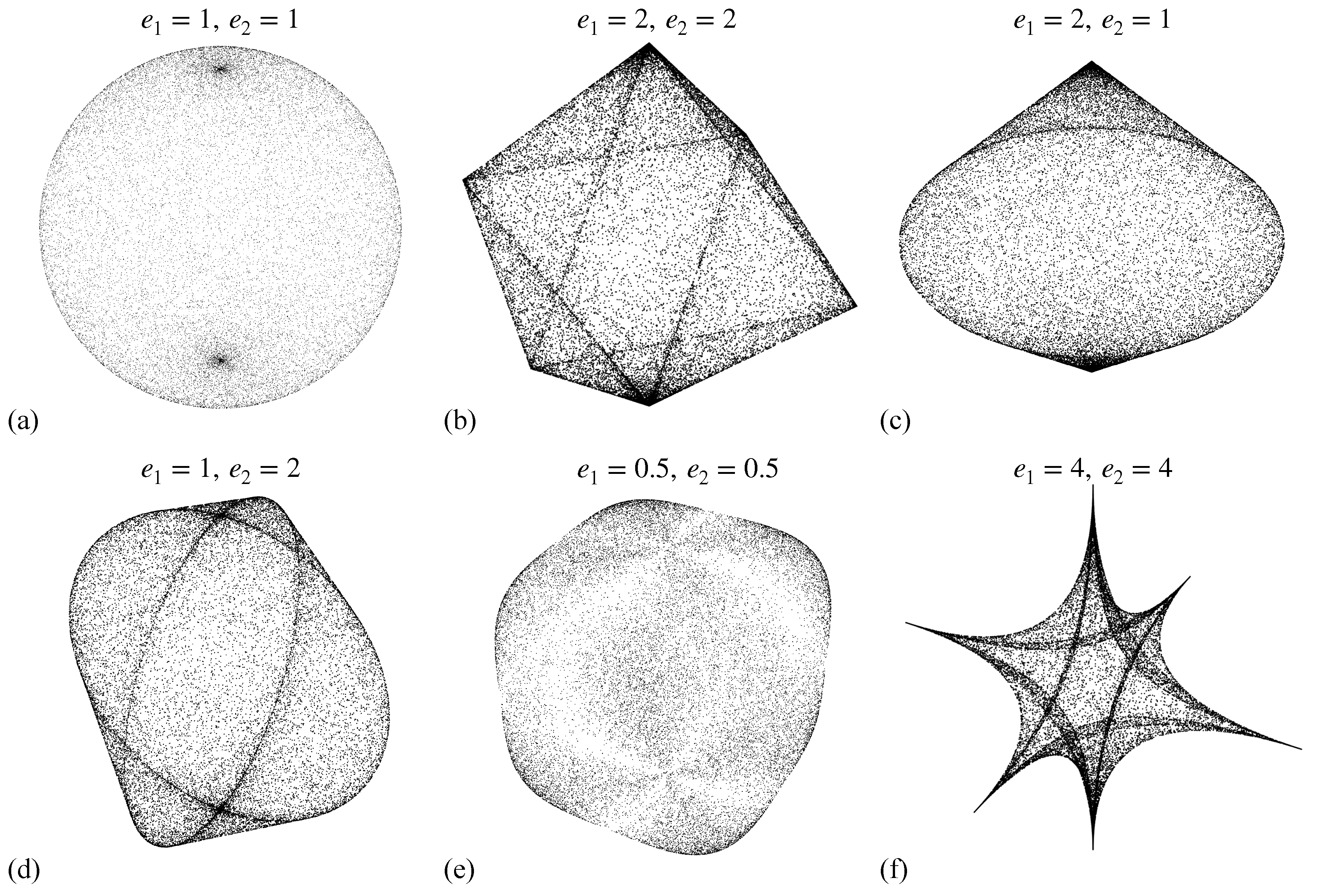
Figure 2.
Small-angle scattering curves for each of the six classes of superquadrics depicted in Figure 1. (a) The simulated pair-distance distribution functions (see main text for details). (b) The scattering intensity, given by Eq. (7). In both cases, the red vertical bars represent errors (the standard deviations for 10 trials, for each class).
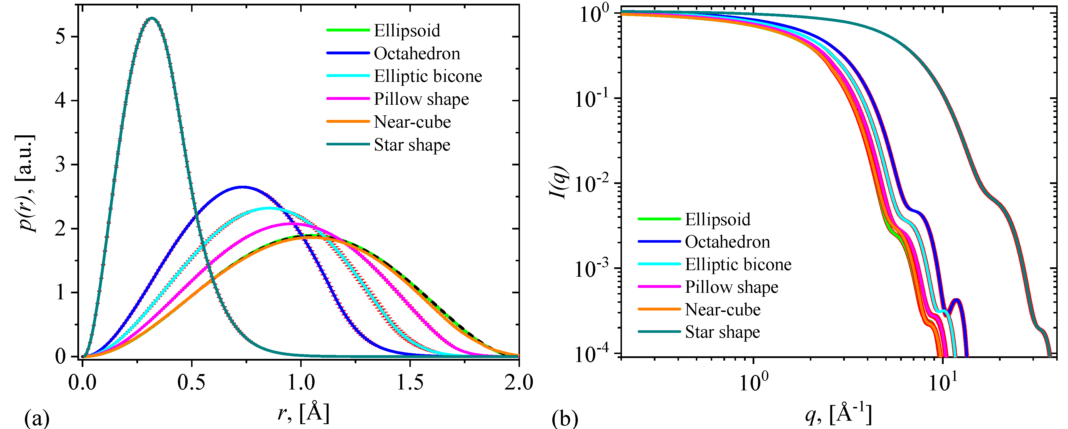
Figure 3.
Guinier plot for each of the six classes of superquadrics depicted in Figure 1. Black dots: calculated data (from Figure 2b) according to Eq. (9), after taking the logarithm. Coloured continuous lines: linear fits. The values of the slopes are given in Tab. Table 1.
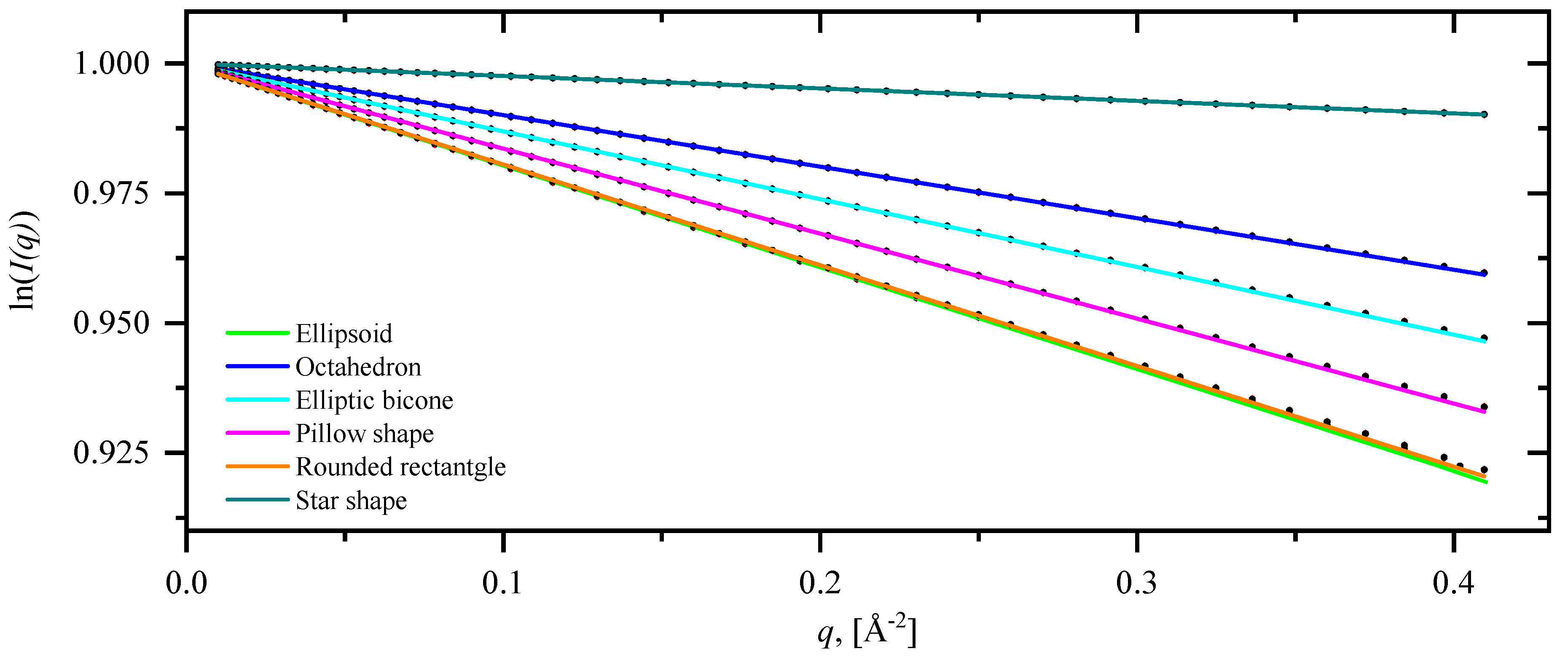
Figure 4.
(a) The structure of chimeric protein complex of ferritin from Helicobacter pylori with N-terminal His6-SUMO-tag [36]. The complex’s domains are shown in different colours. On top of the complex is superimposed a star shape superquadric (transparent light blue colour) with parameters Å, Å, Å, and . (b) The corresponding SAXS experimental scattering intensity, reported in Ref. [36]. Vertical red lines represent measurement errors. Green curve - scattering from the star-like superquadric. Blue line - Guinier’s approximation given by Eq. (9). Horizontal dashed-line is the background (see main text for details).


Table 1.
Structural parameters for each of the six classes of superquadrics depicted in Figure 1. (Å) is the value of r for which attains its maximum, is the slope of the straight lines in Figure 3, and (Å) is the radius of gyration obtained from Eq. (9).
| Ellipsoid | Octahedron | Elliptic bicone | Elliptic pillow | Near-cube | Star | |
|---|---|---|---|---|---|---|
| 1.03 | 0.73 | 0.85 | 0.97 | 1.03 | 0.32 | |
| -0.19 | -0.10 | -0.13 | -0.16 | -0.19 | -0.02 | |
| 0.78 | 0.55 | 0.63 | 0.69 | 0.76 | 0.27 |
Disclaimer/Publisher’s Note: The statements, opinions and data contained in all publications are solely those of the individual author(s) and contributor(s) and not of MDPI and/or the editor(s). MDPI and/or the editor(s) disclaim responsibility for any injury to people or property resulting from any ideas, methods, instructions or products referred to in the content. |
© 2024 by the authors. Licensee MDPI, Basel, Switzerland. This article is an open access article distributed under the terms and conditions of the Creative Commons Attribution (CC BY) license (http://creativecommons.org/licenses/by/4.0/).
Copyright: This open access article is published under a Creative Commons CC BY 4.0 license, which permit the free download, distribution, and reuse, provided that the author and preprint are cited in any reuse.


