
Submitted:
29 July 2024
Posted:
30 July 2024
You are already at the latest version
Abstract
The proliferation of fake news on social media platforms poses significant challenges to information authenticity and public trust. In this study, the impact of various word embedding techniques on the performance of both machine learning and deep learning models for fake news detection is systematically evaluated. The comprehensive TruthSeeker dataset, which spans over a decade of labeled news articles and social media posts, is utilized. Three popular word embedding techniques are analyzed: TF-IDF, Word2Vec, and FastText. These embeddings were tested with multiple machine learning classifiers, including logistic regression, naive Bayes, K-nearest neighbors, support vector machines, multilayer perceptrons, decision trees, and random forests, as well as deep learning models, specifically convolutional neural networks (CNNs). Among machine learning models, the Support Vector Machine (SVM) with TF-IDF achieved the highest accuracy of 99.03%, precision of 98.92%, recall of 99.15%, and F1 score of 99.03%. The Multilayer Perceptron (MLP) also demonstrated strong performance with Word2Vec, reaching an accuracy of 95.24%, precision of 94.95%, recall of 95.50%, and F1 score of 95.07%. For deep learning models, CNNs combined with TF-IDF embeddings showed outstanding results, achieving an accuracy of 98.99%, precision of 98.56%, recall of 99.48%, and F1 score of 99.02%. These results highlight the critical role of word embeddings in enhancing model accuracy and reliability in misinformation detection.
Keywords:
Natural language processing
; Machine learning
; Deep learning
; Fake news detection
; Word embedding.
1. Introduction
The digital age has brought about an unprecedented increase in the availability and dissemination of information. While this has democratized access to knowledge, it has also facilitated the rapid spread of misinformation and fake news. Fake news, defined as false or misleading information presented as news, has become a pervasive problem, influencing public opinion, swaying political outcomes, and even inciting social unrest. The challenge of distinguishing authentic news from fake news is compounded by the sheer volume and velocity at which information propagates through social media and other online platforms [1].
The impact of fake news extends beyond the digital realm, affecting real-world events and undermining trust in traditional media sources. For instance, during the 2016 U.S. presidential election, a surge in fake news stories arguably influenced voter behavior and election outcomes [2]. Another significant example is the 2019 general election in India, where misinformation campaigns on social media platforms sought to sway voters by spreading false narratives and inflammatory content [3]. Similarly, the COVID-19 pandemic witnessed an alarming spread of false information about the virus, treatments, and vaccines, posing significant public health risks [4]. These examples underscore the urgent need for effective mechanisms to detect and combat fake news.
Natural Language Processing (NLP) has emerged as a critical component in the fight against fake news, with word embedding playing a pivotal role. Word embedding is a type of word representation that allows words to be represented as vectors in a continuous vector space. This representation captures semantic relationships between words, such that words with similar meanings have similar vector representations. Techniques such as Term Frequency-Inverse Document Frequency (TF-IDF), Word2Vec, and FastText have revolutionized text processing by providing dense vector representations that improve the ability of algorithms to understand and analyze textual data. These embedding techniques are crucial for enhancing the feature extraction process, enabling models to capture nuanced patterns and relationships in the data [5].
Word embedding significantly impact the performance of both machine learning (ML) and deep learning (DL) models in fake news detection. By providing a more meaningful representation of text data, word embeddings can improve the accuracy and efficiency of these models. However, the choice of word embedding technique can greatly influence the performance of the models [6]. Therefore, it is essential to study the interplay between the selection of the appropriate word embedding technique and how it affects the performance of various ML and DL techniques.
This study aims to explore this interplay by systematically evaluating the impact of different word embedding techniques on the performance of various machine learning and deep learning models in fake news detection. Specifically, this work considers three word embedding techniques: TF-IDF, Word2Vec, and FastText. The objective is to determine which word embedding provides the most significant improvements in accuracy, precision, recall, and F1 score for these models. This evaluation is conducted using the TruthSeeker dataset [7], which encompasses a diverse array of news articles, tweets, and social media posts collected over more than a decade.
The research investigates a range of individual classifiers, including logistic regression, naive Bayes, K-Nearest Neighbors (KNN), support vector machine (SVM), multilayer perceptron (MLP), decision tree, and random forest. Additionally, it evaluates convolutional neural networks (CNNs) as a deep learning model, testing three different network architectures. By leveraging word embedding, this study enhances the feature extraction process, enabling models to capture nuanced patterns in the data.
The main contributions of this work can be summarized as follows:
- Comprehensive Evaluation: The study evaluates the effectiveness of various machine learning and deep learning models for fake news detection using a comprehensive set of performance metrics, including accuracy, precision, recall, and F1 score.
- Word Embedding Impact: The study systematically analyzes the impact of different word embedding techniques (TF-IDF, Word2Vec, and FastText) on the performance of machine learning and deep learning models.
- Rich Dataset Utilization: The TruthSeeker dataset, comprising diverse and temporally extensive data, is utilized to ensure robust training and testing of models.
- Comparative Analysis: The performance of individual classifiers and CNN architectures is compared to identify optimal strategies for fake news detection.
The remainder of this paper is organized as follows: Section 2 summarizes related research efforts, Section 3 presents the utilized research methodology, including data collection and pre-processing, word embedding techniques, machine learning and deep learning implementation, and performance evaluation. Section 4 presents the obtained evaluation results. Section 5 highlights and discusses the main observations drawn from the evaluation results. Finally, Section 6 concludes and summarizes this work.
2. Related Work
In recent years, the detection of fake news on social media platforms has garnered significant attention from researchers. Various approaches have been proposed to tackle this problem, utilizing different machine learning and natural language processing (NLP) techniques. The primary focus of these studies has been on improving the accuracy and robustness of fake news detection systems through innovative methodologies and comprehensive datasets.
The study in [8] employed stochastic neural networks to extract sentiment from Twitter data, integrating natural language processing (NLP) techniques with neural networks (NN). This approach demonstrated the effectiveness of combining sentiment analysis with deep learning for predicting the trends and sentiments in social media posts.
Similarly, the work in [9] developed a content classification and sentiment analysis model using COVID-Twitter-BERT, achieving high classification accuracy across multiple themes. It has highlighted the potential of transformer-based models in capturing the nuances of social media discussions during the COVID-19 pandemic.
Additionally, the framework introduced in [10] utilized Twitter data to generate automated reports on the Russia-Ukraine conflict. This framework leveraged advanced NLP algorithms, including language translation, sentiment analysis, and topic modeling, to provide comprehensive insights into the cyber activities during the conflict.
Moreover, the research in [11] explored sentiment classification using various machine learning algorithms to determine the polarity of textual content. It was demonstrated that the Passive Aggressive (PA) algorithm, combined with a unigram model, outperformed other algorithms in sentiment analysis tasks across multiple datasets.
Furthermore, the application of NLP methods to anomaly detection in log files was investigated in [12], using algorithms such as AdaBoost, Gaussian Naive Bayes, and Random Forest. The study emphasized the importance of selecting appropriate classifiers and feature extraction techniques for effective anomaly detection. The investigation in [13] focused on detecting fake news sources and content on online social networks. It reviewed various text feature extraction techniques and classification algorithms, finding that the Support Vector Machine (SVM) linear classifier using TF-IDF features achieved the highest accuracy in fake news detection.
The research in [14] focused on the classification of fake news by examining different textual properties that distinguish fake from real news. Natural language processing techniques were employed to pre-process the data, subsequently training various machine learning classifiers with all possible combinations of the extracted properties. The results indicated that the Naive Bayes algorithm achieved the best performance, demonstrating the effectiveness of thorough pre-processing and feature combination in enhancing model accuracy.
Graphical methods have also been employed in fake news detection. The study in [15] presented the Factual News Graph (FANG), a learning framework and graphical social context representation aimed at identifying false news. Unlike traditional contextual models, FANG emphasizes representation learning, proving to be efficient at inference time and scalable during training. This approach highlights the importance of integrating social context in fake news detection models.
The word in [16] utilized a graph-based scan technique to identify rumors at the network level, focusing on local anomalies. The rumor detection system detects irregularities in user behavior, post content, and hashtag usage, offering a robust method for identifying rumors based on social media data streams. This method underscores the potential of graph-based approaches in enhancing the accuracy of fake news detection systems.
The research in [17] employed the XGBoost model to determine the significance of various variables in detecting fake news, identifying key factors. Representative machine learning classification models such as SVM, RF, LR, CART, and NNET were then utilized to compare their performance in fake news detection. The study demonstrated the importance of feature importance analysis in improving the accuracy of fake news detection models.
These studies collectively underscore the critical role of advanced NLP and machine learning techniques in enhancing the detection and analysis of fake news on social media platforms. The integration of sentiment analysis, topic modeling, and deep learning algorithms has proven to be particularly effective in capturing the complexities of social media content and improving the accuracy of fake news detection systems.
Existing research in fake news detection highlights two main challenges:
- Dataset Quality: The performance of fake news detection models is significantly impacted by the quality of the datasets used for training and evaluation. The presence of inherent biases or inconsistencies in datasets can hinder model accuracy.
- Model-Representation Instability: An absence of a single, universally effective text representation technique for fake news classification has been observed. The complex and often deceptive nature of fake news content necessitates a multifaceted approach.
In this paper, an approach to address these challenges in fake news classification is proposed. A high-quality, well-established ground truth dataset, TruthSeeker, is leveraged for the training and evaluation of models. Additionally, the efficacy of combining various text representation techniques is explored. By incorporating a diverse range of word embeddings—such as TF-IDF, Word2Vec, and FastText—a more comprehensive representation of the underlying characteristics of fake news is aimed to be captured. Text representation techniques provide valuable insights into the semantic relationships and word usage patterns within news content. This approach empowers the model to learn from a richer information landscape, potentially leading to more robust and generalizable fake news detection capabilities.
The existing work [18] is the closest to our research. While their study utilized the TruthSeeker dataset and employ various machine learning algorithms for fake news detection, this paper the offers a more exhaustive analysis. The previous work primarily focuses on combining handcrafted features with text embedding features, specifically utilizing BERT and RoBERTa, and evaluates their performance across several machine learning models such as Random Forest, AdaBoost, and Support Vector Machine. The results highlight that the integration of these advanced text representations with handcrafted features yields superior performance compared to traditional methods like TF-IDF and Word2Vec . In contrast, our paper extends this research by systematically analyzing the impact of multiple word embedding techniques—TF-IDF, Word2Vec, and FastText—on a broader range of machine learning and deep learning models. This comprehensive evaluation includes not only individual classifiers such as logistic regression, naive Bayes, K-Nearest Neighbors, support vector machine, multilayer perceptron, decision tree, and random forest but also explores the efficacy of various Convolutional Neural Network (CNN) architectures. This study’s extensive use of performance metrics, including accuracy, precision, recall, and F1 score, provides a detailed understanding of how different embeddings influence model performance, identifying the optimal strategies for fake news detection . In summary, our research not only builds on the existing literature by incorporating advanced word embedding techniques and a comprehensive set of performance metrics but also provides a more robust and detailed comparative analysis of various machine learning and deep learning models. This holistic approach marks a significant step forward in the ongoing efforts to improve the accuracy and efficiency of fake news detection systems.
3. Materials and Methods
This section highlights the stages followed in this research including dataset description, dataset pre-processing, word embedding techniques, machine learning and deep learning implementation for fake news detection detection along with performance evaluation. The main steps conducted to evaluate the performance of various machine learning and deep learning techniques are illustrated in Algorithms 1 and 2, respectively.
| Algorithm 1:Tweet Preprocessing and Machine Learning Model Evaluation |
|
3.1. Dataset Description
This research utilizes the TruthSeeker dataset, a groundbreaking resource designed to tackle the challenges of misinformation and fake news on social media. Covering a period from 2009 to 2022, the dataset documents the evolution of online discourse, capturing major global events and the associated rise in misinformation. The TruthSeeker dataset includes over 180,000 tweets, labeled through a meticulous multi-phase process to ensure high accuracy and reliability [7].
Initially, labels were assigned using reputable sources like Politifact and a panel of expert reviewers. This was followed by crowd-sourcing on Amazon Mechanical Turk (MTurk), where each tweet received annotations from three distinct workers. To enhance label robustness, an active learning verification process was employed, involving 456 unique MTurk Master Turkers. This process provided multi-dimensional validation, supporting both binary (real/fake) and multiclass (five-label and three-label) classification schemes. Such rigorous labeling methodologies ensure the dataset supports both basic and nuanced analyses of tweet authenticity.
Beyond simple labels, the TruthSeeker dataset offers extensive auxiliary information that enhances its analytical potential. Each tweet is accompanied by scores reflecting bot likelihood, user credibility, and user influence, providing a comprehensive view of the tweet’s origin and potential impact. These scores are essential for understanding the dynamics of automated misinformation, content source credibility, and the mechanisms through which influential users propagate false information.
| Algorithm 2:Tweet Preprocessing and CNN Model Evaluation |
|
Additionally, the dataset is enriched with detailed metadata, including user profiles, tweet timestamps, and various engagement metrics such as likes, retweets, and replies. This contextual information is invaluable for studying the spread and virality of misinformation, enabling researchers to trace the lifecycle of fake news from inception to dissemination across networks.
Publicly accessible through the Canadian Institute for Cybersecurity (CIC), the TruthSeeker dataset is an open resource for the global research community. Its extensive validation and rich metadata make it a crucial tool for advancing fake news detection research. Researchers can use this dataset to develop and test new machine learning algorithms, study behavioral patterns associated with misinformation, and propose interventions to mitigate its spread.
In summary, the TruthSeeker dataset is a comprehensive, meticulously validated, and richly annotated resource that significantly contributes to understanding and combating misinformation on social media. Its detailed and multi-dimensional nature provides a robust foundation for a wide range of research endeavors aimed at addressing one of the most pressing issues of the digital age.
3.2. Dataset Preprocessing
The prep-rocessing of tweets in this work involves several crucial steps to ensure that the text data is clean and suitable for analysis. These steps are described as follows:
- Text Cleaning: The initial step in the pre-processing pipeline is text cleaning. This involves removing any URLs, special characters, numerical values, emoticons, emojis, mentions, and hashtags from the raw tweet text. The purpose of this step is to eliminate non-alphanumeric characters and other elements that do not contribute to the semantic content of the tweets. Additionally, extra spaces are removed, and the text is trimmed to ensure uniformity. Finally, the entire text is converted to lowercase to standardize the input and treat words with different letter cases as the same word.
- Tokenization: Following text cleaning, the next step is tokenization. Tokenization involves splitting the cleaned text into individual words, also known as tokens. This step is essential for breaking down the text into smaller, processable units that can be analyzed independently. Each token represents a single word, which allows for more granular manipulation and analysis of the text data.
- Stop Word Removal: The final step in the pre-processing pipeline is stop word removal. Stop words are common words such as "the," "and," "in," etc., that appear frequently in the text but do not carry significant meaning or contribute much to the context. Removing these stop words helps to reduce noise and focus on the more informative parts of the text. A predefined list of stop words is used for this purpose, and any token matching a stop word is removed from the text.
These pre-processing steps ensure that the tweet text is clean, tokenized, and stripped of irrelevant components, making it suitable for further analysis and model training.
3.3. Word Embedding Techniques
In the context of text classification and natural language processing, word embedding plays a crucial role in transforming textual data into numerical vectors that machine and deep learning models can interpret. This section discusses three widely used word embedding techniques: Term Frequency-Inverse Document Frequency (TF-IDF), Word2Vec, and FastText, that are used in this work.
3.3.1. Term Frequency-Inverse Document Frequency (TF-IDF)
The Term Frequency-Inverse Document Frequency (TF-IDF) is a statistical measure used to evaluate the importance of a word in a document relative to a collection of documents, or corpus [19]. It combines two metrics: Term Frequency (TF), which measures the frequency of a word in a document, and Inverse Document Frequency (IDF), which measures how unique or rare a word is across the corpus. Mathematically, TF-IDF is defined as:
where:
Here, represents the frequency of term t in document d, is the total number of documents, and is the number of documents containing term t. TF-IDF assigns higher scores to terms that are frequent in a document but rare across the corpus, thus highlighting terms that are more relevant to the specific document.
3.3.2. Word2Vec
Word2Vec is a neural network-based embedding technique that learns vector representations of words by training on a large corpus of text [20]. It generates dense word vectors that capture semantic relationships between words. Word2Vec employs two primary models: Continuous Bag of Words (CBOW) and Skip-gram. The CBOW model predicts a target word based on its context words, while the Skip-gram model predicts context words given a target word. The objective functions for these models are:
where represents the target word, and represent the context words. The resulting word vectors are dense and capture semantic similarities, such that similar words have similar vectors.
3.3.3. FastText
FastText, an extension of Word2Vec developed by Facebook’s AI Research (FAIR) lab, improves word embedding by considering subword information [21]. Instead of learning word vectors directly, FastText represents each word as a bag of character n-grams. This approach allows FastText to generate embeddings for out-of-vocabulary words and capture morphological variations of words. The loss function used in FastText is similar to that of Word2Vec but incorporates subword information:
where represents the embedding vector of context words and represents the embedding vector of the target word. By leveraging subword information, FastText achieves improved performance on tasks involving rare and morphologically rich languages.
3.4. Machine Learning Techniques
In the realm of machine learning, various algorithms offer distinct approaches to classification and prediction tasks. Among these, Naive Bayes (NB) leverages probabilistic methods to classify data based on Bayes’ theorem, while Logistic Regression (LR) provides a robust linear model for binary outcomes. K-Nearest Neighbors (KNN) utilizes distance metrics to classify instances based on their proximity to labeled data. Support Vector Machines (SVM) excel in finding optimal hyperplanes that separate different classes. Multi-Layer Perceptron (MLP), a type of neural network, captures complex patterns through multiple layers of interconnected neurons. Decision Trees (DT) model decisions as a series of hierarchical choices, and Random Forest (RF) aggregates multiple decision trees to improve classification accuracy and robustness. Each of these techniques brings unique strengths to the task of data analysis and classification. This section briefly describes each of these techniques, which are utilized in this work for fake news detection.
- Naive Bayes (NB): Naive Bayes classifiers, based on Bayes’ theorem, are extensively used for text classification tasks. This probabilistic algorithm calculates the likelihood of a class label based on feature probabilities. The assumption of feature independence given the class label simplifies computation, allowing for efficient training and prediction. Despite their practical effectiveness in tasks like spam filtering and sentiment analysis, Naive Bayes classifiers can be sensitive to feature correlations and non-Gaussian class distributions [22].
- Logistic Regression (LR): Logistic Regression is a widely used statistical method for binary classification problems. It models the probability of a binary outcome based on one or more predictor variables by applying a logistic function to a linear combination of the input features. The output probabilities are used to assign class labels, typically using a threshold of 0.5. Logistic Regression is prized for its simplicity, interpretability, and efficiency, making it suitable for large datasets. It provides insights into the relationships between features and the target variable through coefficients that indicate the strength and direction of these relationships. However, Logistic Regression assumes linear relationships between the features and the log-odds of the target variable, which might not capture more complex patterns in the data [23].
- K-Nearest Neighbors (KNN): KNN is a non-parametric algorithm that classifies by determining the majority class among the K nearest neighbors of a data point. Distance metrics like Euclidean or Manhattan distance are used to identify these neighbors, with the majority vote determining the class label. While KNN is simple to implement and effective for multi-class problems, it can become computationally expensive with large datasets and is sensitive to the choice of K and distance metric. Additionally, KNN is affected by the curse of dimensionality, where performance degrades as the number of features increases [24].
- Support Vector Machines (SVMs): SVMs are a versatile classification tool applicable to both binary and one-class problems. They aim to identify the optimal hyperplane that separates different classes while maximizing the margin between them. The choice of kernel functions, such as linear, polynomial, or radial basis function (RBF), enables the modeling of both linear and non-linear relationships. The regularization parameter C adjusts the balance between margin width and classification error, influencing the model’s complexity and performance [25].
- Multilayer Perceptron (MLP): MLP is a feedforward neural network consisting of multiple layers of neurons. MLPs learn complex, non-linear relationships through forward propagation of inputs and backpropagation for error correction. Activation functions like ReLU or sigmoid introduce non-linearity, enabling the network to model intricate patterns. MLPs are effective for high-dimensional data but can be computationally demanding and prone to overfitting if not properly regularized [26].
- Decision Trees (DT): Decision Trees are a well-known machine learning algorithm used for classification tasks. They construct a model in a tree structure, with internal nodes representing feature tests, branches indicating test outcomes, and leaf nodes denoting class labels. The model is developed through recursive partitioning of the feature space, based on the attribute providing the highest information gain. Decision Trees are appreciated for their interpretability and visualization, offering insights into the decision-making process. They can handle both numerical and categorical features and are robust against outliers. However, they are prone to overfitting, especially when the tree is too deep or the dataset is small [27].
- Random Forest (RF): Random Forest is an ensemble learning method that aggregates multiple decision trees to improve classification accuracy. Each tree is trained on a random subset of features and data, with predictions aggregated through majority voting. This approach reduces overfitting by combining diverse trees and provides feature importance scores, aiding in understanding feature contributions to predictions. Random Forest is effective for high-dimensional data, missing values, and outliers, though it can be computationally intensive [28].
3.5. Deep Learning and Convolutional Neural Networks (CNNs)
Deep learning represents a significant advancement in machine learning, characterized by the use of neural networks with multiple layers to model complex patterns in data. Unlike traditional machine learning methods that rely on manually engineered features, deep learning approaches are capable of automatically learning hierarchical feature representations from raw data. This process involves a deep architecture composed of several layers of interconnected neurons, where each layer progressively extracts more abstract features from the input data [29].
Convolutional Neural Networks (CNNs) are a specialized type of deep learning architecture designed to process data with grid-like structures, such as images and text. CNNs utilize convolutional operations to automatically detect and learn local patterns within the input data. This is achieved through the application of convolutional filters, or kernels, which slide over the input to extract relevant features. In the case of text classification, CNNs process sequences of word embeddings, which are dense vector representations of words capturing semantic meaning. Embeddings such as those produced by Word2Vec or TF-IDF transform words into continuous vectors, allowing CNNs to effectively handle textual data [30].
Within a CNN architecture, convolutional layers apply multiple filters to the word embeddings to identify local patterns and features in the text. These filters detect various n-grams or word combinations that are indicative of specific contexts or meanings. After the convolutional layers, pooling layers are employed to downsample the feature maps, reducing their dimensionality while retaining the most important features. Max pooling, a common technique, selects the maximum value from each region of the feature map, thus capturing the most significant features and contributing to the model’s ability to generalize across different text variations.
The output of the pooling layers is flattened and passed through fully connected layers, which integrate the learned features into a single, comprehensive representation. These fully connected layers then perform the classification task, mapping the high-level features to the target categories. By leveraging the hierarchical feature learning capability of CNNs, this approach enables effective extraction and classification of complex patterns in text data.
Overall, CNNs are well-suited for text classification tasks due to their ability to learn and capture intricate patterns through their layered architecture, making them a powerful tool for analyzing and interpreting textual information.
In this work, three distinct Convolutional Neural Network (CNN) architectures have been evaluated to explore the interplay between network design and word embedding techniques for fake news detection Table 1. The models assessed include variations in convolutional layers, pooling strategies, and dropout mechanisms. CNN Model 1 features a straightforward architecture with a single convolutional layer followed by max pooling, designed to capture basic patterns in the text. CNN Model 2 incorporates additional complexity with batch normalization and global max pooling, aiming to improve feature extraction and model generalization. CNN Model 3 utilizes multiple convolutional and pooling layers to enhance the ability to capture hierarchical patterns in the data. Each model was tested with TF-IDF, Word2Vec, and FastText embeddings to determine which combination yields the highest performance in terms of accuracy, precision, recall, and F1 score. The results provide insights into how different CNN configurations interact with varying embeddings to optimize fake news detection.
3.6. Performance Measures
Evaluating the efficacy of machine and deep learning models in the context of fake news detection involves a comprehensive assessment using several performance metrics. These metrics provide critical insights into the models’ capabilities in accurately identifying false and genuine news articles, ensuring that the detection system is both effective and reliable.
- Accuracy quantifies the overall effectiveness of a model by measuring the proportion of correctly classified instances, including both true positives (TP) and true negatives (TN), relative to the total number of instances. It indicates the model’s general performance but may not fully capture its effectiveness in detecting fake news if class distributions are imbalanced.
- Precision assesses the model’s ability to correctly identify fake news articles, minimizing the rate of false positives (FP). It is particularly important in scenarios where false alarms are costly, as it measures the ratio of true positives to the total number of instances flagged as fake news.
- Recall evaluates the model’s capability to detect all actual fake news instances. It calculates the proportion of true positives among the total number of actual fake news articles, including those that were missed (false negatives, FN). High recall ensures that the majority of fake news articles are identified, which is crucial for minimizing the risk of overlooked false information.
-
F1 Score provides a balanced measure of a model’s precision and recall by computing their harmonic mean. This metric is especially useful in fake news detection to balance the trade-off between precision and recall, ensuring that neither false positives nor false negatives dominate the evaluation.where:
- –
- denotes the number of true positives, representing correctly identified fake news articles.
- –
- denotes the number of true negatives, indicating correctly classified genuine news articles.
- –
- denotes the number of false positives, representing genuine articles incorrectly classified as fake news.
- –
- denotes the number of false negatives, indicating fake news articles that were incorrectly classified as genuine.
4. Results
4.1. Machine Learning Results
Figure 1 illustrates the performance of various machine learning algorithms on fake news detection, under the TF-IDF word embedding technique. The performance of various machine learning algorithms on fake news detection using the TF-IDF word embedding technique showcases notable differences. The Support Vector Machine (SVM) achieved the highest accuracy at 99.03%, along with the highest precision, recall, and F1 score, indicating its superior performance among the models tested. The Multilayer Perceptron (MLP) also performed well, with an accuracy of 98.77% and high precision and recall values. Logistic Regression showed strong performance with an accuracy of 97.58% and balanced precision and recall. Random Forest demonstrated a robust performance with an accuracy of 98.39%, while Decision Tree achieved an accuracy of 97.30%. Naive Bayes had the lowest accuracy at 94.55%, but still maintained reasonable precision and recall values. Overall, SVM and MLP were the top performers, followed by Logistic Regression and Random Forest, with Naive Bayes lagging behind in terms of accuracy.
On the other hand, Figure 2 depicts the performance of various machine learning algorithms on fake news detection using the Word2Vec word embedding technique. The results indicate significant variations in performance among the different algorithms. The Multilayer Perceptron (MLP) achieved the highest accuracy of 95.24%, accompanied by the highest recall and F1 score, demonstrating its strong capability in detecting fake news. The K-Nearest Neighbors (KNN) also performed impressively with an accuracy of 94.98% and high precision and F1 score. Random Forest showed solid results with an accuracy of 91.01%, while Support Vector Machine (SVM) achieved an accuracy of 94.47%. Logistic Regression had a lower accuracy of 85.42% but still maintained reasonable performance metrics. Decision Tree had the lowest accuracy at 80.30%, with comparatively lower precision, recall, and F1 score. Overall, MLP and KNN were the top performers under the Word2Vec embedding, followed by SVM and Random Forest, with Logistic Regression and Decision Tree lagging behind in terms of accuracy.
The performance of various machine learning algorithms on fake news detection using the FastText word embedding technique presents another set of observations, as shown in Figure 3. The Multilayer Perceptron (MLP) achieved the highest accuracy at 93.21%, along with the highest precision and F1 score, indicating its strong capability in detecting fake news. The Support Vector Machine (SVM) performed well with an accuracy of 90.41%, while K-Nearest Neighbors (KNN) showed an accuracy of 85.10% with reasonable precision and recall values. Logistic Regression had an accuracy of 83.44%, showing balanced performance metrics. Random Forest demonstrated an accuracy of 84.53%, while Decision Tree had the lowest accuracy at 72.42%. Overall, MLP and SVM were the top performers under the FastText embedding, followed by KNN and Random Forest, with Logistic Regression and Decision Tree lagging behind in terms of accuracy.
4.2. Deep Learning Results
4.2.1. Learning Curves Comparison
The training of three different CNN models with TF-IDF, Word2Vec and Fasttext embedding techniques for fake news detection demonstrates various trends and observations in accuracy and training loss over the epochs, as shown in Figure 4, Figure 5, and Figure 6.
Figure 4 illustrates the learning curves of the three CNN models under the TF-IDF word embedding techniques, the main observations draw from this figure can be summarized as follows:
- CNN Model 1(Figure 4): The training of CNN Model 1 with TF-IDF embedding showed a consistent and significant improvement in both accuracy and reduction in loss over the epochs. Initially, the model began with an accuracy of 95.63% and a loss of 0.1187. As the training progressed to the second epoch, there was a notable improvement, with accuracy increasing to 98.17% and the loss decreasing to 0.0534. This positive trend continued in the third epoch, where accuracy reached 98.81% and the loss further dropped to 0.0351. By the fourth epoch, the model’s accuracy had improved to 99.14%, accompanied by a reduction in loss to 0.0255. Moving into the fifth epoch, the accuracy climbed to 99.30%, and the loss fell to 0.0198. In the sixth epoch, there was a slight increase in accuracy to 99.37%, with the loss further reducing to 0.0175. The seventh epoch saw the model achieving an accuracy of 99.50%, while the loss was further reduced to 0.0139. During the eighth epoch, the accuracy was 99.51%, with a minimal loss of 0.0135. By the ninth epoch, accuracy had increased to 99.59%, and the loss had decreased to 0.0112. Finally, in the tenth epoch, the model achieved its highest accuracy of 99.62% with a loss of 0.0106.
- CNN Model 2 (Figure 4): The training of CNN Model 2 with TF-IDF embeddings presented a different pattern, starting with a significantly lower accuracy of 51.23% and a higher loss of 0.6935. In the second epoch, the model showed a slight improvement with an accuracy of 51.62% and a reduction in loss to 0.6914. By the third epoch, the accuracy had increased to 51.99% and the loss had decreased to 0.6901. The fourth epoch observed a more substantial increase in accuracy to 52.75% and a decrease in loss to 0.6892. The fifth epoch saw the accuracy rise to 53.27% and the loss reduce to 0.6882. In the sixth epoch, accuracy improved to 53.59% with a corresponding loss decrease to 0.6864. The seventh epoch achieved an accuracy of 54.44% and a loss of 0.6850. By the eighth epoch, the accuracy was 55.06%, with the loss decreasing to 0.6827. The ninth epoch saw a slight decrease in accuracy to 54.97%, but a reduction in loss to 0.6821. Finally, in the tenth epoch, the model attained its highest accuracy of 55.56% with a loss of 0.6807.
- CNN Model 3 (Figure 4): The training of CNN Model 3 with TF-IDF embedding displayed a strong performance throughout, starting with an initial accuracy of 95.58% and a loss of 0.1157. In the second epoch, the model showed a significant improvement, with accuracy increasing to 98.66% and the loss reducing to 0.0401. The third epoch saw a further increase in accuracy to 99.34% and a substantial drop in loss to 0.0206. By the fourth epoch, the accuracy had improved to 99.55% and the loss had decreased to 0.0136. The fifth epoch saw the accuracy rise to 99.73% with a loss of 0.0087. In the sixth epoch, the accuracy further improved to 99.77% with a corresponding loss decrease to 0.0068. The seventh epoch achieved an accuracy of 99.82% and a loss of 0.0051. By the eighth epoch, the accuracy was 99.85% with the loss decreasing to 0.0047. The ninth epoch saw a minimal increase in accuracy to 99.85%, with a slight reduction in loss to 0.0044. Finally, in the tenth epoch, the model achieved its highest accuracy of 99.89% with a loss of 0.0033.
The training of three different CNN models with Word2Vec embedding for fake news detection exhibits distinct patterns and trends in accuracy and training loss over the epochs, as shown in Figure 5:
- CNN Model 1 (Figure 5): The training of CNN Model 1 with Word2Vec embedding displayed a steady improvement in both accuracy and reduction in loss over the epochs. Initially, the model started with an accuracy of 86.53% and a loss of 0.3176. By the second epoch, accuracy increased to 89.54% and the loss decreased to 0.2563. This positive trend continued, with the third epoch showing an accuracy of 90.55% and a loss of 0.2322. In the fourth epoch, the accuracy rose to 91.19% and the loss dropped to 0.2201. The fifth epoch saw further improvement, with accuracy reaching 91.49% and the loss falling to 0.2098. In the sixth epoch, accuracy increased to 91.82% and the loss decreased to 0.2029. The seventh epoch saw an accuracy of 92.10% and a loss of 0.1939. By the eighth epoch, the accuracy was 92.29% with a loss of 0.1896. The ninth epoch showed an accuracy of 92.52% and a loss of 0.1852. Finally, in the tenth epoch, the model achieved an accuracy of 92.65% with a loss of 0.1803.
- CNN Model 2 (Figure 5): The training of CNN Model 2 with Word2Vec embedding showed a different pattern, beginning with an accuracy of 82.53% and a loss of 0.3892. In the second epoch, the model’s accuracy increased to 87.65% while the loss decreased to 0.2982. The third epoch demonstrated an accuracy of 89.19% and a loss of 0.2680. By the fourth epoch, accuracy had improved to 90.07% and the loss had dropped to 0.2478. The fifth epoch saw the accuracy rise to 90.58% and the loss decrease to 0.2343. In the sixth epoch, accuracy reached 91.12% with a loss of 0.2219. The seventh epoch showed an accuracy of 91.39% and a loss of 0.2139. By the eighth epoch, the accuracy improved to 91.94% and the loss reduced to 0.2022. The ninth epoch saw the accuracy increase to 92.20% and the loss drop to 0.1959. Finally, in the tenth epoch, the model achieved its highest accuracy of 92.52% with a loss of 0.1877.
- CNN Model 3 (Figure 5): The training of CNN Model 3 with Word2Vec embedding displayed a noticeable performance throughout. The model began with an accuracy of 86.73% and a loss of 0.3117. By the second epoch, accuracy improved to 90.50% and the loss decreased to 0.2361. The third epoch showed an accuracy of 91.87% and a loss of 0.2057. In the fourth epoch, accuracy reached 92.71% and the loss dropped to 0.1860. The fifth epoch saw an accuracy of 93.30% with a loss of 0.1722. In the sixth epoch, accuracy improved to 93.74% and the loss decreased to 0.1605. The seventh epoch achieved an accuracy of 94.04% with a loss of 0.1535. By the eighth epoch, the accuracy was 94.29% with a loss of 0.1448. The ninth epoch saw an accuracy of 94.58% and a loss of 0.1372. Finally, in the tenth epoch, the model achieved its highest accuracy of 94.89% with a loss of 0.1324.
The training of three different CNN models with FastText embedding for fake news detection demonstrates distinct patterns and trends in accuracy and training loss over the epochs, as shown in Figure 6:
- CNN Model 1 (Figure 6): The training of CNN Model 1 with FastText embedding displayed a steady improvement in both accuracy and reduction in loss over the epochs. Initially, the model started with an accuracy of 80.93% and a loss of 0.4217. By the second epoch, accuracy increased to 83.75% and the loss decreased to 0.3695. This positive trend continued, with the third epoch showing an accuracy of 84.81% and a loss of 0.3485. In the fourth epoch, the accuracy rose to 85.39% and the loss dropped to 0.3336. The fifth epoch saw further improvement, with accuracy reaching 85.98% and the loss falling to 0.3245. In the sixth epoch, accuracy increased to 86.25% and the loss decreased to 0.3181. The seventh epoch saw an accuracy of 86.61% and a loss of 0.3107. By the eighth epoch, the accuracy was 87.08% with a loss of 0.3035. The ninth epoch showed an accuracy of 87.12% and a loss of 0.2999. Finally, in the tenth epoch, the model achieved an accuracy of 87.28% with a loss of 0.2970.
- CNN Model 2 (Figure 6): The training of CNN Model 2 with FastText embeddings showed a different pattern, beginning with an accuracy of 75.28% and a loss of 0.5063. In the second epoch, the model’s accuracy increased to 80.91% while the loss decreased to 0.4249. The third epoch demonstrated an accuracy of 82.70% and a loss of 0.3957. By the fourth epoch, accuracy had improved to 83.67% and the loss had dropped to 0.3770. The fifth epoch saw the accuracy rise to 84.37% and the loss decrease to 0.3628. In the sixth epoch, accuracy reached 84.97% with a loss of 0.3516. The seventh epoch showed an accuracy of 85.67% and a loss of 0.3399. By the eighth epoch, the accuracy improved to 85.89% and the loss reduced to 0.3317. The ninth epoch saw the accuracy increase to 86.18% and the loss drop to 0.3253. Finally, in the tenth epoch, the model achieved its highest accuracy of 86.54% with a loss of 0.3174.
- CNN Model 3 (Figure 6): The training of CNN Model 3 with FastText embedding displayed a relatively moderate performance throughout. The model began with an accuracy of 80.96% and a loss of 0.4155. By the second epoch, accuracy improved to 84.50% and the loss decreased to 0.3548. The third epoch showed an accuracy of 85.88% and a loss of 0.3301. In the fourth epoch, accuracy reached 86.67% and the loss dropped to 0.3119. The fifth epoch saw an accuracy of 87.30% with a loss of 0.2992. In the sixth epoch, accuracy improved to 87.69% and the loss decreased to 0.2889. The seventh epoch achieved an accuracy of 88.25% with a loss of 0.2802. By the eighth epoch, the accuracy was 88.47% with a loss of 0.2725. The ninth epoch saw an accuracy of 88.72% and a loss of 0.2674. Finally, in the tenth epoch, the model achieved its highest accuracy of 88.99% with a loss of 0.2618.
4.2.2. Performance Evaluation Results
Figure 7 shows the testing performance of the studied CNN models under three different word embedding techniques. The performance metrics of accuracy, precision, recall, and F1 score for three different CNN models under the three embedding techniques (TF-IDF, Word2Vec, and FastText) reveal distinct differences and trends in their effectiveness for text classification tasks.
Figure 7 illustrates the testing accuracy values for each combination of CNN model and word embedding technique. For the TF-IDF embedding, CNN Model 1 and Model 3 performed exceptionally well with accuracy values of 98.77% and 98.99%, respectively, indicating their robustness. Conversely, CNN Model 2 showed poor performance with an accuracy of 56.15%. With Word2Vec embedding, CNN Model 3 achieved the highest accuracy at 94.92%, followed closely by CNN Model 1 at 94.25%, and CNN Model 2 slightly lower at 90.73%. Using FastText embeddings, the accuracies were comparatively lower, with CNN Model 3 and Model 1 attaining accuracies around 89.55% and 89.32%, respectively, and CNN Model 2 slightly lower at 85.26%.
On the other hand, Figure 7 shows the precision results. For the TF-IDF embeddings, CNN Model 1 and Model 3 exhibited high precision with values of 98.65% and 98.56%, respectively. CNN Model 2 had a lower precision of 55.69%. With Word2Vec embedding, CNN Model 3 achieved the highest precision at 94.64%, followed by CNN Model 1 at 93.69%, and CNN Model 2 with a precision of 87.13%. For FastText embedding, precision was somewhat lower compared to TF-IDF and Word2Vec, with CNN Model 3 reaching 88.60%, CNN Model 1 at 88.34%, and CNN Model 2 slightly higher at 88.49%.
In addition, Figure 3 illustrates the testing recall values. For TF-IDF embeddings, CNN Model 3 achieved the highest recall of 99.48%, followed by CNN Model 1 at 98.97%. CNN Model 2 had a lower recall of 70.93%. With Word2Vec embedding, CNN Model 2 attained the highest recall of 96.13%, followed by CNN Model 3 and Model 1 with recalls of 95.50% and 95.20%, respectively. With FastText embeddings, CNN Model 3 had the highest recall of 88.72%, with CNN Model 1 at 91.21%, and CNN Model 2 at 81.90%.
Furthermore, The F-1 scores are depicted in Figure 7. For the TF-IDF embeddings, CNN Model 3 achieved the highest F1 score of 99.02%, followed by CNN Model 1 at 98.81%, while CNN Model 2 had a much lower F1 score of 62.39%. With Word2Vec embeddings, CNN Model 3 led with an F1 score of 95.07%, closely followed by CNN Model 1 at 94.44%, and CNN Model 2 at 91.41%. Using FastText embeddings, CNN Model 3 had the highest F1 score of 89.96%, with CNN Model 1 at 89.75%, and CNN Model 2 at 85.07%.
5. Discussion
The comparative analysis of machine learning algorithms on fake news detection using three different word embedding techniques—TF-IDF, Word2Vec, and FastText—reveals several important insights. Overall, the Multilayer Perceptron (MLP) and Support Vector Machine (SVM) consistently emerged as the top performers across all embedding techniques. Specifically, MLP achieved the highest accuracy and performance metrics with Word2Vec at 95.24% and FastText at 93.21%, while SVM excelled with TF-IDF at 99.03%.
On the other hand, the TF-IDF embedding technique generally resulted in higher accuracy and performance metrics across most models compared to Word2Vec and FastText. This indicates that TF-IDF is more effective in capturing the relevant features for fake news detection, thus enhancing model performance. Conversely, Decision Tree consistently exhibited the lowest performance across all three embedding techniques, with the lowest accuracy observed with FastText at 72.42%.
Furthermore, Logistic Regression and Random Forest demonstrated balanced but comparatively lower performance metrics than MLP and SVM, showing variability in accuracy depending on the embedding technique used. In particular, Logistic Regression achieved 97.58% accuracy with TF-IDF but showed lower performance with Word2Vec and FastText.
In summary, the choice of word embedding technique significantly impacts the performance of machine learning models in fake news detection. While TF-IDF generally provides the highest performance across most models, MLP and SVM consistently perform well regardless of the embedding technique employed. These findings underscore the importance of selecting appropriate embedding techniques to optimize the efficacy of machine learning algorithms in detecting fake news.
In evaluating the performance of CNN models with various word embeddings, CNN Model 3 with TF-IDF embeddings stands out as the top performer across all metrics. This combination achieved the highest accuracy (98.99%), precision (98.56%), recall (99.48%), and F1 score (99.02%), showcasing its exceptional classification capabilities. Following closely is CNN Model 1 with TF-IDF embeddings, which also delivered outstanding results with an accuracy of 98.77%, precision of 98.65%, recall of 98.97%, and F1 score of 98.81%. This makes CNN Model 1 with TF-IDF embeddings the second best performer overall. For stability, CNN Model 3 with Word2Vec embedding is notable for its consistent high performance, achieving an accuracy of 94.92%, precision of 94.64%, recall of 95.50%, and F1 score of 95.07%. Thus, CNN Model 3 with TF-IDF embedding is the preferred choice for achieving both the highest performance and stability, with CNN Model 1 with TF-IDF embedding being a close and highly competitive option.
6. Conclusions
The detection of fake news has become increasingly critical in today’s digital age, where misinformation can spread rapidly through social media and other online platforms. This study comprehensively evaluated the impact of different word embedding techniques on the performance of machine learning and deep learning models for fake news detection. Utilizing the TruthSeeker dataset, which spans over a decade of labeled news articles and social media posts, the effectiveness of three popular word embedding techniques—TF-IDF, Word2Vec, and FastText—was explored. These embedding techniaues were tested with a range of machine learning classifiers, including logistic regression, naive Bayes, K-nearest neighbors, support vector machines, multilayer perceptrons, decision trees, and random forests, as well as deep learning models, specifically convolutional neural networks (CNNs).
It was found that the choice of word embedding technique significantly impacts the performance of fake news detection models. Among the machine learning models, the Support Vector Machine (SVM) combined with TF-IDF embedding achieved the highest performance metrics, with an accuracy of 99.03%, precision of 98.92%, recall of 99.15%, and F1 score of 99.03%. The Multilayer Perceptron (MLP) also demonstrated strong performance with Word2Vec embedding, achieving an accuracy of 95.24%, precision of 94.95%, recall of 95.50%, and F1 score of 95.07%. These results underscore the robustness of SVM and MLP models when paired with appropriate word embedding.
For deep learning models, CNNs combined with TF-IDF embedding showed outstanding results, achieving an accuracy of 98.99%, precision of 98.56%, recall of 99.48%, and F1 score of 99.02%. This demonstrates the superior capability of CNNs in capturing complex patterns in text data when enhanced by effective word embedding. The importance of selecting suitable word embedding techniques to optimize the performance of deep learning models in the context of fake news detection is thus highlighted.
The comparative analysis reveals that TF-IDF generally provides the highest performance across most models compared to Word2Vec and FastText. This suggests that TF-IDF embedding is particularly effective in capturing the relevant features for fake news detection, thereby enhancing overall model performance. However, Word2Vec and FastText also showed competitive results, especially when used with deep learning models, indicating their potential utility in specific contexts.
In summary, the critical role of word embedding in enhancing the accuracy and reliability of machine learning and deep learning models for fake news detection has been highlighted. The need for careful selection of embedding techniques to achieve optimal model performance is emphasized. Future research could explore the integration of more advanced embedding techniques and hybrid models to further improve fake news detection capabilities. Additionally, expanding the scope to include ensemble methods and incorporating textual, lexical, and metadata features could provide a more holistic approach to combating misinformation.
Author Contributions
Conceptualization, Mutaz A. B. Al-Tarawneh, Omar Al-irr, and Khaled Al-Maaitah; methodology, Mutaz A. B. Al-Tarawneh and Khaled Al-Maaitah; software, Mutaz A. B. Al-Tarawneh and Khaled Al-Maaitah; validation, Mutaz A. B. Al-Tarawneh, Omar Al-irr, Khaled Al-Maaitah, and Wael Hosny Fouad Aly; formal analysis, Mutaz A. B. Al-Tarawneh and Khaled Al-Maaitah; investigation, Mutaz A. B. Al-Tarawneh and Khaled Al-Maaitah; resources, Mutaz A. B. Al-Tarawneh and Khaled Al-Maaitah; data curation, Mutaz A. B. Al-Tarawneh and Khaled Al-Maaitah; writing—original draft preparation, Mutaz A. B. Al-Tarawneh; writing—review and editing, Mutaz A. B. Al-Tarawneh, Omar Al-irr, Khaled Al-Maaitah, Hassan Kanj, and Wael Hosny Fouad Aly; visualization, Mutaz A. B. Al-Tarawneh; supervision, Mutaz A. B. Al-Tarawneh, Khaled Al-Maaitah, and Hassan Kanj; project administration, Mutaz A. B. Al-Tarawneh. All authors have read and agreed to the published version of the manuscript.
Funding
“Not applicable”
Institutional Review Board Statement
“Not applicable”.
Informed Consent Statement
“Not applicable”.
Data Availability Statement
The data supporting the findings of this study are available within the article. The TruthSeeker dataset, which was utilized in this study, is publicly accessible through the Canadian Institute for Cybersecurity (CIC) at https://www.cic.unb.ca/datasets/truthseeker.html. This dataset includes extensive metadata and auxiliary information used for analysis. Additional data and materials related to this study are available from the corresponding author upon reasonable request. No new data were created specifically for this study.
Acknowledgments
Machine and deep learning training and evaluation have been performed using the Phoenix High Performance Computing facility at the American University of the Middle East, Kuwait.
Conflicts of Interest
The authors declare no conflicts of interest.
Abbreviations
The following abbreviations are used in this manuscript:
| Conv1D | Convolutional 1D |
| ReLU | Rectified Linear Unit |
| CNN | Convolutional Neural Network |
| TF-IDF | Term Frequency-Inverse Document Frequency |
| MLP | Multilayer Perceptron |
| SVM | Support Vector Machine |
| KNN | K-Nearest Neighbors |
| RF | Random Forest |
| DT | Decision Tree |
| NB | Naive Bayes |
| LR | Logistic Regression |
References
- Olan, F.; Jayawickrama, U.; Arakpogun, E.O.; Suklan, J.; Liu, S. Fake news on Social Media: the Impact on Society. Information Systems Frontiers 2024, 26, 443–458. [Google Scholar] [CrossRef] [PubMed]
- Allcott, H.; Gentzkow, M. Social Media and Fake News in the 2016 Election. Journal of Economic Perspectives 2017, 31, 211–236. [Google Scholar] [CrossRef]
- Gupta, A.; Roy, A. Manipulation of Social Media during the 2019 Indian General Elections. Asian Journal of Communication 2019, 29, 537–556. [Google Scholar]
- Cinelli, M.; Galeazzi, A. The COVID-19 social media infodemic. Scientific Reports 2020, 10, 1–10. [Google Scholar] [CrossRef] [PubMed]
- Meesad, P. Thai Fake News Detection Based on Information Retrieval, Natural Language Processing and Machine Learning. SN Computer Science 2021, 2, 425. [Google Scholar] [CrossRef] [PubMed]
- Asudani, D.S.; Nagwani, N.K.; Singh, P. Impact of word embedding models on text analytics in deep learning environment: a review. Artificial Intelligence Review 2023, 56, 10345–10425. [Google Scholar] [CrossRef] [PubMed]
- Dadkhah, S.; Zhang, X.; Weismann, A.G.; Firouzi, A.; Ghorbani, A.A. The Largest Social Media Ground-Truth Dataset for Real/Fake Content: TruthSeeker. IEEE Transactions on Computational Social Systems 2024, 11, 3376–3390. [Google Scholar] [CrossRef]
- di Tollo, G.; Andria, J.; Filograsso, G. The Predictive Power of Social Media Sentiment: Evidence from Cryptocurrencies and Stock Markets Using NLP and Stochastic ANNs. Mathematics 2023, 11. [Google Scholar] [CrossRef]
- Xie, T.; Ge, Y.; Xu, Q.; Chen, S. Public Awareness and Sentiment Analysis of COVID-Related Discussions Using BERT-Based Infoveillance. AI 2023, 4, 333–347. [Google Scholar] [CrossRef]
- Sufi, F. Social Media Analytics on Russia–Ukraine Cyber War with Natural Language Processing: Perspectives and Challenges. Information 2023, 14. [Google Scholar] [CrossRef]
- Gamal, D.; Alfonse, M.M.; El-Horbaty, E.S.; M. Salem, A.B. Analysis of Machine Learning Algorithms for Opinion Mining in Different Domains. Machine Learning and Knowledge Extraction 2019, 1, 224–234. [Google Scholar] [CrossRef]
- Ryciak, P.; et al. Anomaly detection in log files using selected natural language processing methods. Applied Sciences 2022, 12, 5089. [Google Scholar] [CrossRef]
- Hisham, M.; Hasan, R.; Hussain, S. An Innovative Approach for Fake News Detection using Machine Learning. Sir Syed University Research Journal of Engineering and Technology 2023, 13, 115–124. [Google Scholar] [CrossRef]
- Khanam, Z.; Alwasel, B.; Sirafi, H.; Rashid, M. Fake News Detection Using Machine Learning Approaches. IOP Conference Series: Materials Science and Engineering 2021, 1099, 012040. [Google Scholar] [CrossRef]
- Nguyen, V.H.; Sugiyama, K.; Nakov, P.; Kan, M.Y. Leveraging Social Context for Fake News Detection Using Graph Representation. In Proceedings of the Proceedings of the 29th ACM International Conference on Information & Knowledge Management; 2020; pp. 1165–1174. [Google Scholar]
- Tam, N.T.; Weidlich, M.; Zheng, B.; Yin, H.; Hung, N.Q.V.; Stantic, B. From Anomaly Detection to Rumor Detection Using Data Streams of Social Platforms. Proceedings of the VLDB Endowment 2019, 12, 1016–1029. [Google Scholar] [CrossRef]
- Park, M.; Chai, S. Constructing a User-Centered Fake News Detection Model by Using Classification Algorithms in Machine Learning Techniques. IEEE Access 2023, 11, 71517–71527. [Google Scholar] [CrossRef]
- Khalil, M.; Azzeh, M. Fake news detection models using the largest social media ground-truth dataset (TruthSeeker). International Journal of Speech Technology 2024. [Google Scholar] [CrossRef]
- Dai, S.; Li, K.; Luo, Z.; Zhao, P.; Hong, B.; Zhu, A.; Liu, J. AI-based NLP section discusses the application and effect of bag-of-words models and TF-IDF in NLP tasks. Journal of Artificial Intelligence General science (JAIGS) ISSN:3006-4023 2024, 5, 13–21. [Google Scholar] [CrossRef]
- Johnson, S.J.; Murty, M.R.; Navakanth, I. A detailed review on word embedding techniques with emphasis on word2vec. Multimedia Tools and Applications 2024, 83, 37979–38007. [Google Scholar] [CrossRef]
- Umer, M.; Imtiaz, Z.; Ahmad, M.; Nappi, M.; Medaglia, C.; Choi, G.S.; Mehmood, A. Impact of convolutional neural network and FastText embedding on text classification. Multimedia Tools and Applications 2023, 82, 5569–5585. [Google Scholar] [CrossRef]
- Dharta, F.Y.; Januar Mahardhani, A.; Rachmawati Yahya, S.; Dirsa, A.; Usulu, M. Application of Naive Bayes Classifier Method to Analyze Social Media User Sentiment Towards the Presidential Election Phase. Jurnal Informasi Dan Teknologi 2024, 6, 176–181. [Google Scholar] [CrossRef]
- Leukel, J.; Özbek, G.; Sugumaran, V. Application of logistic regression to explain internet use among older adults: a review of the empirical literature. Universal Access in the Information Society 2024, 23, 621–635. [Google Scholar] [CrossRef]
- Zhang, J.; Li, Y.; Shen, F.; He, Y.; Tan, H.; He, Y. Hierarchical text classification with multi-label contrastive learning and KNN. Neurocomputing 2024, 577, 127323. [Google Scholar] [CrossRef]
- El-Rashidy, M.A.; Mohamed, R.G.; El-Fishawy, N.A.; Shouman, M.A. An effective text plagiarism detection system based on feature selection and SVM techniques. Multimedia Tools and Applications 2024, 83, 2609–2646. [Google Scholar] [CrossRef]
- Rashedi, K.A.; Ismail, M.T.; Al Wadi, S.; Serroukh, A.; Alshammari, T.S.; Jaber, J.J. Multi-Layer Perceptron-Based Classification with Application to Outlier Detection in Saudi Arabia Stock Returns. Journal of Risk and Financial Management 2024, 17. [Google Scholar] [CrossRef]
- Reusens, M.; Stevens, A.; Tonglet, J.; De Smedt, J.; Verbeke, W.; vanden Broucke, S.; Baesens, B. Evaluating text classification: A benchmark study. Expert Systems with Applications 2024, 254, 124302. [Google Scholar] [CrossRef]
- Kanahuati-Ceballos, M.; Valdivia, L.J. Detection of depressive comments on social media using RNN, LSTM, and random forest: comparison and optimization. Social Network Analysis and Mining 2024, 14, 44. [Google Scholar] [CrossRef]
- Taye, M.M. Understanding of Machine Learning with Deep Learning: Architectures, Workflow, Applications and Future Directions. Computers 2023, 12. [Google Scholar] [CrossRef]
- Li, Z.; Liu, F.; Yang, W.; Peng, S.; Zhou, J. A Survey of Convolutional Neural Networks: Analysis, Applications, and Prospects. IEEE Transactions on Neural Networks and Learning Systems 2022, 33, 6999–7019. [Google Scholar] [CrossRef]
Figure 1.
Machine learning model performance - TF-IDF.
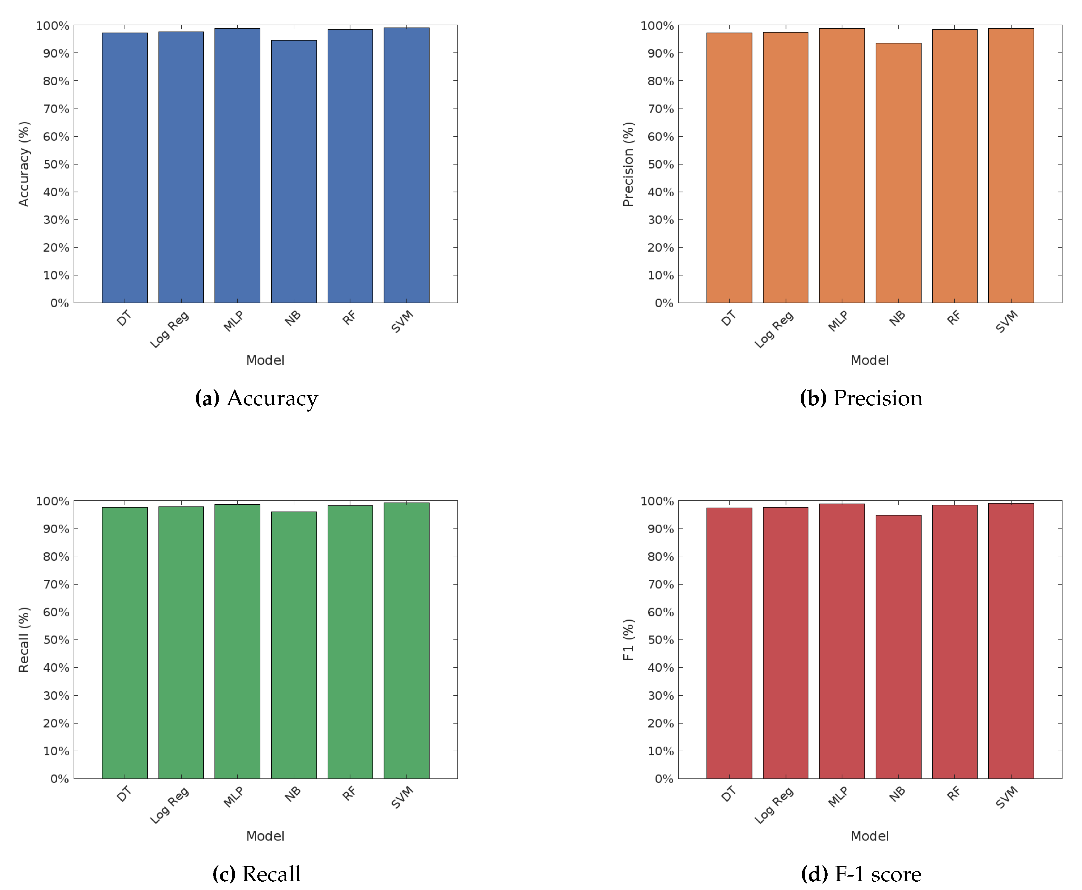
Figure 2.
Machine learning model performance - Word2Vec.
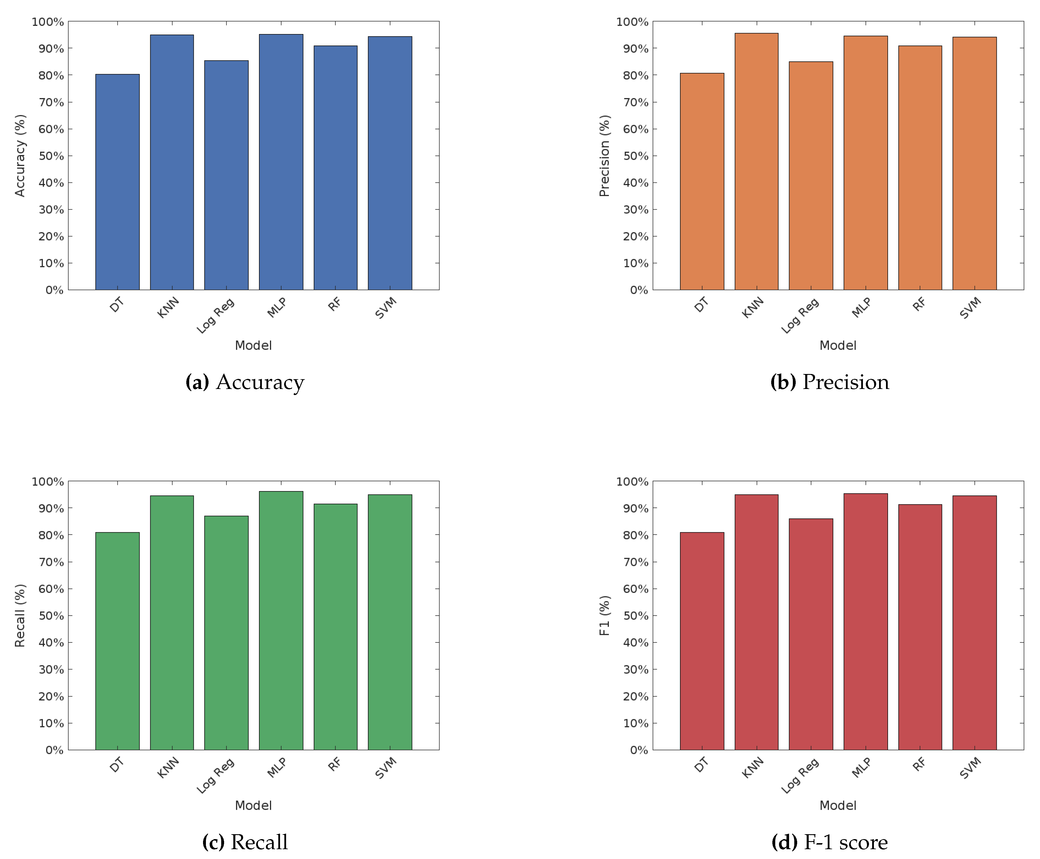
Figure 3.
Machine learning model performance - FastText

Figure 4.
CNN Models Learning Curves under TF-IDF.
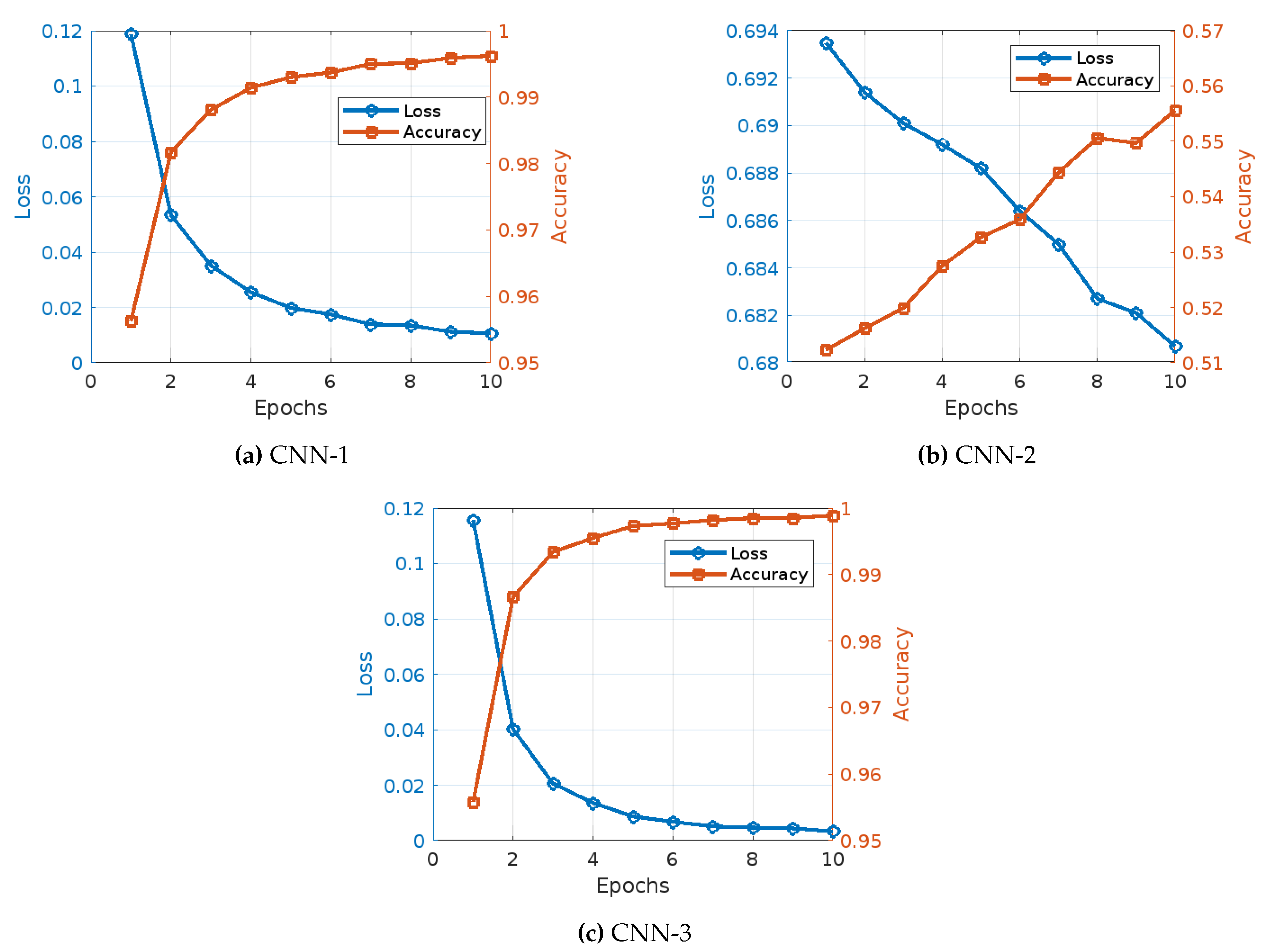
Figure 5.
CNN Models Learning under Word2Vec.
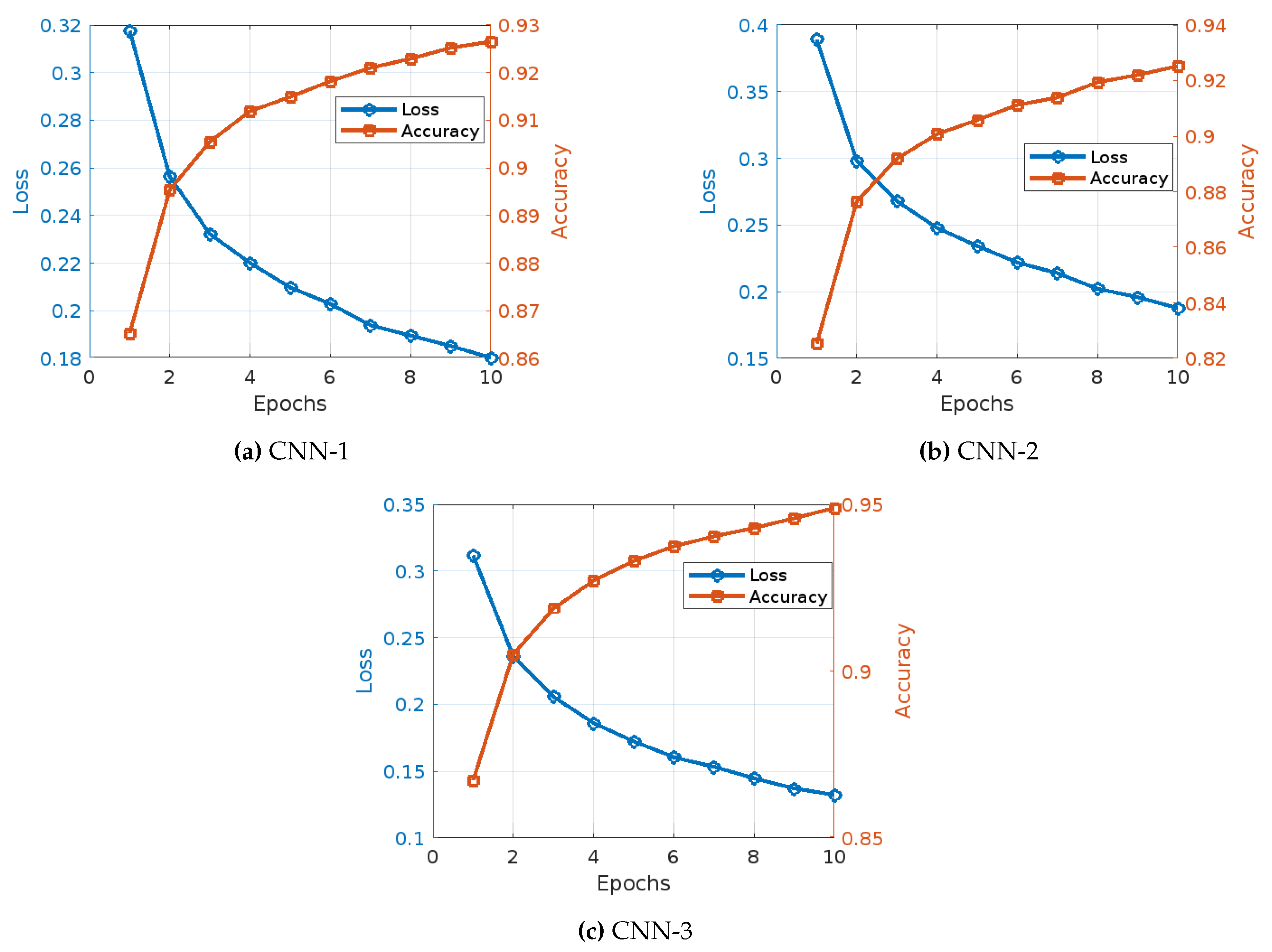
Figure 6.
CNN Models Learning Curves under Fasttext.
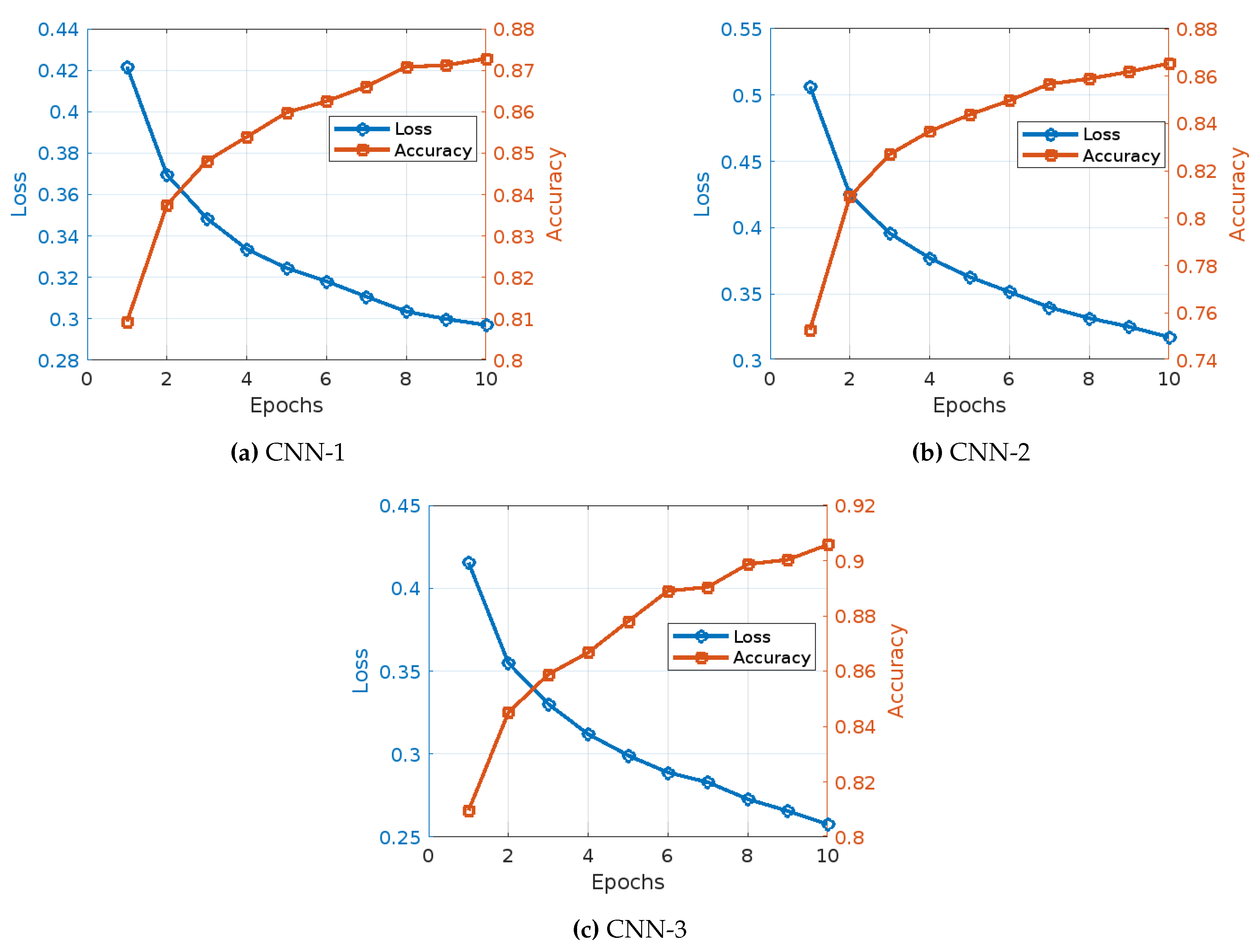
Figure 7.
CNN models performance comparison.
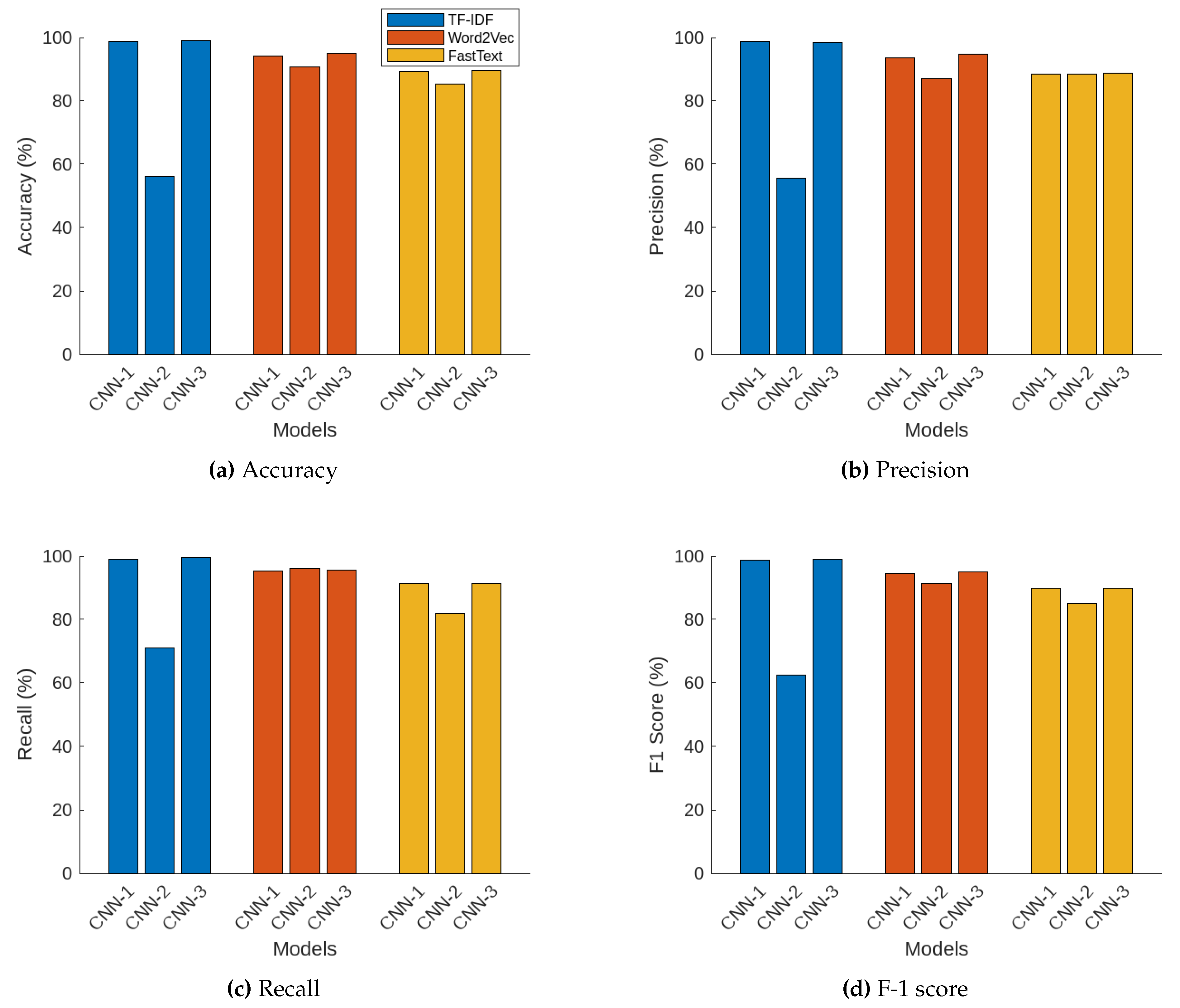

Table 1.
Summary of Convolutional Neural Network (CNN) Models.
| Model | Layer Type | Filters | Kernel Size | Activation | Other Details |
|---|---|---|---|---|---|
| CNN Model 1 | Conv1D | 128 | 5 | ReLU | MaxPooling1D (pool size=2) |
| Flatten | - | - | - | Dense (64 units, ReLU) | |
| Dropout | - | - | - | Dropout (0.5) | |
| Dense (Output) | - | - | Sigmoid | ||
| CNN Model 2 | Conv1D | 64 | 5 | ReLU | BatchNormalization |
| MaxPooling1D | - | 2 | - | Conv1D (128 filters, 5 kernel size) | |
| GlobalMaxPooling1D | - | - | - | Dense (64 units, ReLU) | |
| Dropout | - | - | - | Dropout (0.5) | |
| Dense (Output) | - | - | Sigmoid | ||
| CNN Model 3 | Conv1D | 32 | 3 | ReLU | MaxPooling1D (pool size=2) |
| Conv1D | 64 | 3 | ReLU | MaxPooling1D (pool size=2) | |
| Flatten | - | - | - | Dense (128 units, ReLU) | |
| Dropout | - | - | - | Dropout (0.5) | |
| Dense (Output) | - | - | Sigmoid |
Disclaimer/Publisher’s Note: The statements, opinions and data contained in all publications are solely those of the individual author(s) and contributor(s) and not of MDPI and/or the editor(s). MDPI and/or the editor(s) disclaim responsibility for any injury to people or property resulting from any ideas, methods, instructions or products referred to in the content. |
© 2024 by the authors. Licensee MDPI, Basel, Switzerland. This article is an open access article distributed under the terms and conditions of the Creative Commons Attribution (CC BY) license (http://creativecommons.org/licenses/by/4.0/).
Copyright: This open access article is published under a Creative Commons CC BY 4.0 license, which permit the free download, distribution, and reuse, provided that the author and preprint are cited in any reuse.


