
Submitted:
23 July 2024
Posted:
25 July 2024
You are already at the latest version
Abstract
We conducted a multi-scaled Ecoregional Conservation Assessment for the Southern Rockies (~14.5M ha) and its trailing edge, the Santa Fe Subregion (~2.2M ha), Wyoming to New Mexico, USA. We included a representation analysis of Existing Vegetation Types (EVT), mature-old-growth forests (MOG), and four focal species—Canada lynx (Lynx canadensis), North American wolverine (Gulo gulo luscus), Mexican spotted owl (Strix occidentalis lucida), and northern goshawk (Accipiter gentilis)—in relation to 30 x 30 and 50 x 50 conservation targets. To integrate conservation targets with wildfire risk reduction to the built environment and climate change planning, we overlaid the location of wildfires and forest treatments in relation to the Wildland-Urban Interface (WUI) and included downscaled climate projections for a lower (RCP4.5) and higher (RCP8.5) emissions scenario. Protected areas were highly skewed toward upper elevation EVTs (most were >50% protected), underrepresented forest types (<30% protected), especially MOG (<22% protected) and riparian areas (~14% protected), and poorly represented habitat (<30%) for at least 3 of the focal species, especially in the subregion where nearly all the targets underperformed compared to the ecoregion. Most (>73%) forest thinning treatments over the past decade were >1-km from delineated WUI areas, well beyond the distance at which vegetation management can effectively reduce structure ignition risk (< 50-m from structures). Extreme heat, drought, snowpack reductions, altered timing of peak stream flows, increasing wildfires, and potential shifts in the climate niche of woodlands over conifer forests may impact forest dependent species, while declining snowpack may impact wolverine that den in upper elevations. Strategically targeting the built environment for fuel treatments would improve wildfire risk reduction and may allow for expansion of protected areas held up in controversy. Stepped-up protections for roadless areas, adoption of wilderness proposals, and greater protections for MOG and riparian forests are critical for meeting representation targets.
Keywords:
biodiversity
; climate change
; ecoregion
; conservation
; Santa Fe
; Southern Rockies
1. Introduction
The Southern Rocky Mountains Ecoregion (SRME) spans ~14.5M ha of a rugged terrain characterized by abrupt transitions from many of the tallest peaks (>3,660 m) in North America to expansive lowland-valleys primarily within portions of southern Wyoming, central and western Colorado, and northern New Mexico, USA [1,2]. A prominent feature is the Continental Divide that splits the Pacific (to the west) and Atlantic (to the east) drainages. Beta diversity is especially pronounced across elevational life zones, with distinct shifts in species assemblages traversing lower montane/foothills, upper montane, subalpine, and alpine areas [1,3]. The World Wildlife Fund considered the ecoregion the Colorado Rockies Forests (Ecoregion #45) and ranked it “bioregionally outstanding” and “relatively stable” due mainly to large intact areas, including national parks, Wilderness areas, and Inventoried Roadless Areas (IRAs) [1,4]. NatureServe listed the ecoregion as the Southern Rocky Mountain Montane Forest & Woodland Macrogroup [M022; 5]. The USDA Forest Service identified five distinct subsections, including the Northern Parks and Ranges, South-Central Highlands, Northern-Central Highlands and Rocky Mountains, Southern Parks and Rocky Mountain Ranges, and Northern Rio Grande Basin [3]. Within the SRME, some 184 plant and animal species are endemic, 100 are globally imperiled (G1-G2), 23 are listed under the Endangered Species Act, and seven have been extirpated [1,3]. Importantly, species reintroductions have taken place in portions of the ecoregion, including Mexican gray wolf (Canis lupus), bison (Bison bison), black-footed ferret (Mustela nigripes), river otter (Lutra canadensis) and Canada lynx (Felis lynx canadensis, in Colorado), with a wolverine (Gulo gulo luscus) reintroduction program recently approved in Colorado that will begin soon (Colorado Senate Bill 24-171; https://leg.colorado.gov/bills/sb24-171; accessed May 25, 2024).
Large-scale conservation proposals (e.g., 30% protected by 2030, “30 x 30”; 50% protected by 2050, “50 x 50”) [6] are a cornerstone of conservation biology approaches worldwide [7] as well as of long-standing conservation efforts in this ecoregion [1,3,8,9]. For instance, The Nature Conservancy identified 188 conservation priority areas totaling 50% of the SRME to meet conservation goals of targeted species, natural, and ecological systems [3]. In the Southern Rockies, protected areas may function as important climate refugia with relatively low climate velocities compared to their developed surroundings [9], especially where there are large roadless area complexes, wilderness areas, and national parks [1,8].
Notably, the trailing edge of ecoregions may be especially vulnerable to higher climate velocities because species assemblages and climatic conditions are at their margins. A case in point is the Santa Fe Subregion (SFSR) at the southern edge of the SRME that climatically differs from the rest of the ecoregion via seasonal monsoons that affect natural disturbance dynamics. Climate change related shifts in monsoon delivery may affect the onset and length of the wildfire season [10]. The SFSR also includes a dense population center nearby, Santa Fe, that has experienced periodic wildfires in the surroundings with some wildfires spilling into nearby communities that abut the two primary national forests in this subregion: the Santa Fe and Carson (a small portion of the Rio Grande National Forest in Colorado is also included in SFSR). The Santa Fe National Forest is closest to numerous homes in harm’s way of wildfires. The overwhelming response by the USDA Forest Service has been unprecedented aerial fire suppression along with expansive forest thinning and burning proposed by researchers (e.g., prescribed fire and pile burning) [11,12,13,14] as well as road building to access sites for vegetation management. There is scientific debate and public controversy about whether such aggressive fuel reduction treatments are an effective strategy in a changing climate [15], the cumulative ecosystem damages associated with some of the treatments [16], whether too much forest biomass is being removed and too frequently [17], whether fire-risk reduction for communities should instead target areas closest to homes [18,19], the smoke and human health risks of frequent and extensive prescribed burns, and prescribed fires that sometimes escape containment (e.g., Calf Canyon/Hermit’s Peak fire of 2022) [20]. Importantly, The Nature Conservancy identified ~46% of the Santa Fe National Forest as a priority for coarse and fine-filter conservation [21]. However, little progress has been made toward these broader conservation targets mainly due to the controversy over forest management and wildfires.
Our objective is to present a multi-scaled Ecoregional Conservation Assessment (ECA) that incorporates conservation needs of both the larger SRME and the SFRS nested within it. Multi-scaled ECAs are necessary to ensure that a particular area of interest (subregion) is contextually analyzed for its relative conservation contributions within the backdrop of climate change, forest management, and wildfires. It is also necessary to demonstrate that large-scale conservation (e.g. priority areas, focal species distributions) can be compatible with wildfire risk reduction to the built environment and climate change planning.
We selected Canada lynx, a federally threatened species under the US Endangered Species Act; wolverine, federally threatened; northern goshawk (Accipiter gentilis), a USDA Forest Service “sensitive species;” and Mexican spotted owl (Strix occidentalis lucia), federally threatened, to represent a mixture of forest conservation and landscape connectivity needs at the two spatial scales (ecoregion, subregion), and to compare levels of protection of these focal species between the two scales using 30% and 50% targets. ECAs that include both landscape and focal species can be useful in advancing conservation proposals in regions facing multiple threats from development, wildland fires affecting towns, climate change, and controversial forest management practices. Our ECA approach to the SRME builds on a related ECA for the Mogollon Highlands in Arizona, just to the southeast that is facing some of the same conflicts over protection vs. forest management and wildfire risks [22]. ECAs like these may provide a means to advance conservation in high fire-risk environments where protected area proposals have stalled due to land management agencies and/or elected official calls for increased forest management via logging, burning, and road building.
2. Materials & Methods
2.1. Study Area
We used EPA Level III ecoregional classifications [2] to map the SRME study area (i.e., EPA Ecoregion 21) and overlaid a climate change projection boundary based on study area grid coordinates in the Climate Toolbox online portal (climatetoolbox.org; accessed May 3, 2024) (Figure 1). The study area boundary was confirmed by regional experts in a May 2024 workshop. For the purpose of a continuous ecoregional analysis, we did not include small, isolated fragments in Utah that are, despite their discontinuity, considered part of EPA Ecoregion 21.
Watershed boundaries were overlaid on the study area using 4-digit Hydrologic Unit Codes [HUC; 23] of the ecoregion and 8-digit HUCs for the SFSR in order to provide the necessary detail for a scaled-analysis. We delineated the SFSR as the 10 southernmost 8-digit HUCs in the SRME (Table S1) (Figure 1). All spatial analyses were conducted at both the SRME and SFSR scale. Based on our mapping approach, the SRME totaled 14,475,519 ha and the SFSR was 2,188,050 ha (~15% of the SRME) (Figure 1).
We clipped all spatial datasets to the study area and re-projected to a CONUS Albers projection (EPSG:5070) using QGIS version 3.36 (https://qgis.org). To reduce processing time, we converted most of our vector datasets to 30-m raster datasets aligned with LANDFIRE (2022, LF 2.3.0) rasters such as the elevation dataset that we used to create Figure 1. This allowed us to combine rasters representing different metrics, each having a set of unique pixel values corresponding to surface ownership, vegetation type, forest structure class, etc. The only exceptions to this raster approach were our analyses involving wolverine habitat connectivity as well as the analyses involving USDA Forest Service thinning activities that were both conducted using clipped vector datasets.
2.2. Landowners and GAP Status
For the Wyoming and New Mexico portions of the SRME, we used surface landowner data from the PAD-US 3.0. For the Colorado portion of the SRME (which comprises the majority of the ecoregion), we extracted landowner data from the Colorado Ownership Management and Protection Map (COMaP, v20230223) as it has greater accuracy than the PAD-US across the state. We grouped landowner polygons into nine ownership categories for all analyses that involved surface ownership. We also included National Forest Boundaries from the USDA Forest Service Enterprise Data Warehouse as described in DellaSala et al. [22].
We extracted US Geological Survey (USGS) GAP Analysis Project (GAP) status codes 1-4 from the PAD-US supplemented with data from the National Conservation Easement Database (NCEDB). We combined USDA Forest Service IRA data from the national dataset (2001 Roadless Area Conservation Rule) for IRAs in New Mexico and Wyoming and from the 2012 Colorado Roadless Rule dataset for IRAs in Colorado (https://www.fs.usda.gov/main/roadless/coloradoroadlessrules; accessed May 10, 2024). The Colorado Roadless Rule differs from the 2001 national rule as it classified portions of IRAs as either “upper tier” or “non-upper tier.” Upper tier IRAs have even greater protections than those under the national rule (e.g. in Wyoming or New Mexico), so we assigned upper tiers as GAP 2. We assigned IRAs in Wyoming and New Mexico as well as non-upper tier IRAs in Colorado GAP 2.5 as these areas have enhanced protections beyond what is typical for GAP 3 lands (see [22]). Because the PAD-US data combined with IRA and NCEDB data include overlapping polygons, our final GAP status dataset represents the lowest GAP status code (i.e. the highest level of protection) for any given area. Any areas outside of this combined dataset were assigned GAP 4. We combined the final GAP status rasters with rasters for the metrics below to determine the proportion of each area (e.g. Canada lynx suitable habitat) in each GAP status.
We obtained Wilderness area boundaries in several proposed federal legislation efforts that we had spatial data for, including the Colorado Wilderness Act, Colorado Outdoor Recreation and Environment Act, Gunnison Outdoor Resources Protection Act, and the Sarvis Creek Wilderness Completion Act (a total of 210,486 ha proposed as Wilderness in these bills). We created a separate GAP status dataset with existing Wilderness boundaries adjusted and new Wilderness areas added assuming all these bills were signed into law. We then calculated the GAP status distribution across the SRME and SFSR under this scenario.
2.3. Existing Vegetation Types (2020 Update)
We accessed Existing Vegetation Type (EVT) data for the study area using LANDFIRE (2022, LF 2.3.0) that represents the current distribution of terrestrial ecological systems developed by NatureServe for the western hemisphere. There were 97 EVTs within the SRME (Table S2), which we grouped into 19 broader categories, with a focus on the forest types most likely used by our focal species, including Alpine, Aspen (Populus spp) and Mixed-Conifer Forest, Aspen Forest and Woodland, Lodgepole Pine (Pinus contorta) Forest, Mixed-Conifer Forest, Pinyon (Pinus spp.)-Juniper (Juniperus spp.), Ponderosa Pine, and Subalpine Forest. The EVTs within the SFSR were generally similar to those of the ecoregion as described by Vander Lee et al. [21] with some noted exceptions such as the lack of lodgepole pine forest and limber pine woodland.
Characteristic tree species in the study area include Engelmann spruce (Picea engelmannii), blue spruce (Picea pungens), subalpine fir (Abies lasiocarpa), Rocky Mountain Douglas-fir (Pseudotsuga menziesii var. glauca), Rocky Mountain white fir (Abies concolor subsp. concolor), Rocky Mountain bristlecone pine (Pinus aristata), limber pine (Pinus flexilis), lodgepole pine, Ponderosa pine (Pinus ponderosa), Colorado pinyon pine (Pinus edulis), Rocky Mountain juniper (Juniperus scopulorum), and gambel oak (Quercus gambelii). Interestingly, southwestern white pine (Pinus strobiformis) and limber pine commingle at or near the limits of their geographical ranges to form a unique hybrid zone in the SFSR [24]. Riparian areas are characterized by abundant forbs and shrubs (when not grazed by cattle), narrowleaf cottonwood (Populus angustifolia), quacking aspen (Populus tremuloides), Plains cottonwood (Populus deltoides), peachleaf willow (Salix amygdaloides), Rocky Mountain maple (Acer grandidentatum), and thinleaf alder (Alnus tenuifolia) (see [4]). Alpine zones (above tree line) support a variety of shrubs, wildflowers, krummholz (stunted trees) and many non-vascular plants on exposed rocks [2].
2.4. Mature and Old-growth Forests (MOG)
We obtained spatial datasets on mature and old-growth (MOG) forest distributions from DellaSala et al. [25], who used three proxies to define MOG at 30m-resolution: tree height, canopy coverage, and above-ground biomass. As in DellaSala et al. [25], we grouped the nine forest structure classes in this dataset into three broader categories: young, intermediate, and mature forests. Because some of the proxy data used to create the original MOG dataset were obtained several years prior, we determined that the dataset needed to be screened for relatively recent high-severity fire events to ensure that we did not consider areas with greater than about 75% tree mortality from fire as MOG. We extracted high-severity fire data from the four-class composite burn index (CBI-4) annual mosaics, 2012 through 2023, in the USDA Forest Service Rapid Assessment of Vegetation Condition after Wildfire (RAVG) database and censored out any overlapping MOG pixels from our final analyses and maps (https://burnseverity.cr.usgs.gov/ravg/data-access, accessed April 14, 2024)
Using the RAVG mosaics allowed us to include fire severity data from the 2022 Hermits Peak/Calf Canyon Fire, which burned a substantial portion of the SFSR but which was not yet included in the Monitoring Trends in Burn Severity (MTBS) dataset. Data for some fires in the earlier years of the annual mosaic range were affected by the Landsat 7 Scan Line Corrector error. Any areas within the mosaics that were within the swaths lacking data due to this well-known error were also censored from the final MOG dataset.
2.5. Focal Species
2.5.1. Wolverine
Wolverine occupy isolated subalpine areas at low population densities and have been used to model metapopulation dynamics and landscaped connectivity with dispersing animals following low-resistance pathways that connect high-quality habitat [26]. We used a habitat connectivity dataset provided by Carroll et al. [26] via Data Basin, who used Circuitscape 4.0 to produce habitat connectivity scores for the western U.S. at an approximately 25-km resolution. We clipped this raster dataset to the SRME, then extracted the raster pixels with connectivity scores at the 90th percentile or above and again at the 95th percentile or above for the ecoregion. We converted these two sets of extracted pixels to vector formats and then clipped our GAP vector layer to them and calculated the GAP distribution for each dataset. We did this again for the SFSR, but the 90th and 95th percentile values were still based on the entire SRME.
2.5.2. Canada Lynx, Northern Goshawk, and Mexican Spotted Owl
Canada lynx use mid-elevation boreal and subalpine zones with deep snowpack, selecting forests with a high proportion of beetle-killed large trees and with high horizontal cover used by its principal prey species, snowshoe hare (Lepus americanus) [27]. Northern goshawk select mature forests with large trees and high canopy closure [28] and in parts of their range will nest in dense aspen and lodgepole pine forests [29]. The Mexican spotted owl typically uses forests with high canopy cover in mixed-conifer and pine-oak forests and woodlands and is known to be sensitive to habitat fragmentation [30].
We used the 2001 GAP Analysis Project habitat suitability dataset (30-m resolution) for each of the three species. Because of the age of these datasets, we censored out any suitable habitat pixels that have experienced high-severity fire from 2001-2023, which is a conservative approach that ensures suitable habitat distribution was not overestimated. We extracted high-severity pixels from RAVG annual mosaics for the 2012-2023 period as described in the MOG section above. We then extracted the high-severity class of pixels from the MTBS annual fire severity raster mosaics for the 2001-2011 period (RAVG data were not available for the region prior to 2012) and combined these with the high-severity fire pixels from the RAVG dataset to create a mask layer that we used to censor out any suitable habitat pixels in the 2001 GAP Analysis datasets. We combined our censored habitat suitability datasets with the GAP status datasets for both the SRME and SFSR to calculate the GAP status distributions for each species’ total area of suitable habitat.
2.6. Wildland-Urban Interface/Intermix (WUI), Wildfires, and Forest Thinning
We extracted the six 2020 categories of WUI areas from the national WUI dataset produced by Radeloff et al. [31]: low-density intermix, medium-density intermix, high-density intermix, low-density interface, medium-density interface, and high-density interface. We rasterized the dataset as we did with other datasets above and combined it with our GAP status raster for both the SRME and SFSR.
We extracted all wildfires from the MTBS national dataset from 1984-2022, amended with the final fire perimeter for the 2022 Hermits Peak/Calf Canyon Fire, and then dissolved these perimeters to delineate the portions of the SRME and SFSR that burned at least once during that time period. We did not analyze fire severity distributions as that was beyond the scope of this study. We rasterized the fire footprint data as described previously and combined it with our GAP status raster as well as our WUI raster. We also created a raster denoting existing Wilderness, upper tier IRAs in Colorado, and non-upper tier Colorado IRAs as well as IRAs in Wyoming and New Mexico and then combined this with the fire footprint raster.
To determine where mechanical thinning operations have been taking place on national forest land in the SRME and SFSR, relative to WUI areas, we extracted from the USDA Forest Service’s Forest Activities Tracking System (FACTS) database (https://data.fs.usda.gov/geodata/edw/datasets.php, accessed April 18, 2024) all activity polygons with a completion date during or after 2014 and before 2024 and which had a treatment type of “thinning” in the hazardous fuels dataset in FACTS, or an activity name of “commercial thinning” in the timber harvest dataset in FACTS, or an activity name of “precommercial thinning” in the timber stand improvement dataset in FACTS. We merged and dissolved these polygons to delineate the 2014-2023 mechanical thinning footprint in national forests across the SRME and SFSR. Next, we dissolved our WUI dataset and added to it four buffer zones at 250-m increments from the edge of any WUI outer boundary. We then intersected our thinning footprint vector dataset with these buffer zones to determine the area and percentage that was conducted within 250-m, 500-m, 750-m, 1-km, and >1-km of a WUI area.
2.7. Downscaled Climate Projections
Extreme topographic relief of the Rockies (Figure 1) drives much of the climatic variability within the SRME. The climate is considered temperate semiarid steppe regime with annual average temperatures ranging from 1.6° to 7.2° C reaching 10° C in low-lying valleys [3]. Eastern slopes are much drier due to the montane rain-shadow. Late-summer monsoonal precipitation is characteristic of the SFRS [10]. Annual precipitation overall ranges from <254-mm at the base of mountains to >1.4-m at higher elevations, primarily as snowfall [3].
We used the Climate Toolbox online portal (climatetoolbox.org; accessed May 3, 2024) to project potential climate change scenarios for the study area, which includes a collection of web tools visualizing past and present climate and vegetation of the contiguous U.S. Methods, data, and sources for the many different tools are available on the Climate Toolbox website. We calculated historical trends using the “Historical climate tracker” tool, delineated with a rectangle that encompassed the entire study area (see Figure 1). For future climate trend projections across the study area, we input a custom shapefile in the Climate Toolbox portal. In general, future projections were more precisely delineated than historical climate assessment.
Historical values were calculated using the gridMET dataset, which is a gridded surface meteorological dataset covering the continental U.S. from 1979-present, mapping surface weather variables at ~4 km spatial grain [32]. Future projections were produced using Multivariate Adaptive Constructed Analogs (MACA) version 2 output, based on an ensemble of 20 GCMs (bcc-cs1-1, bcc-csm1-1-m, BNU-ESM, CanESM2, CCSM4, CNRM-CN5, CSIRO-Mk3-6-0, GFDL-ESM2M, GFDL-ESM2G, HADGem2-CC365, HADGem2-ES365, inmcm4, IPSL-CM5A-LR, IPSL-CM5A-MR, IPSL-CM5B-LR, MIROC5, MIROC-ESM, MIROC-ESM-CHEM, MRI-CGCM3, NorESM1-M) and 2 scenarios (RCP 4.5 and 8.5) that were downscaled to a ~4 km resolution for compatibility with the gridMET data [32].
We accessed output from the MC2 dynamic global vegetation model [33,34] through the Climate Toolbox Future Vegetation web tool. MC2 was forced with downscaled MACAv2-PRISM data. Historical and future vegetation data, which are sourced from the Integrated Scenarios Project (https://consbio.org/projects/integrated-scenarios-of-climate-hydrology-and-vegetation-for-the-northwest/; accessed May 3, 2024) were used to simulate potential vegetation change based on climate variables. High uncertainty in these projections stems from numerous non-modeled factors such as species dispersal capabilities, competition among species, and natural successional dynamics.
We accessed streamflow projections through the Climate Toolbox Future Streamflows web tool, also sourced from the Integrated Scenarios Project (https://consbio.org/projects/integrated-scenarios-of-climate-hydrology-and-vegetation-for-the-northwest/; accessed May 3, 2024). Streamflow data were generated from the non-regulated stream routing of VIC (version 4.1.2) hydrologic outputs, utilizing large-scale river routing scheme [35] and forced with MACAv2-LIVNEHv13 downscaling of the CMIP5 global climate model outputs.
3. Results
3.1. Landownerships and Gap Status
Nearly half (48.5%) of the 14.5M ha SRME is managed by the USDA Forest Service, 34% is private surface ownership, 8.2% is by the US Bureau of Land Management (BLM), 3.9% is by various state agencies, 2.9% is by Native American tribes, 1.3% is by the National Park Service, and the remainder is managed by multiple agencies and entities (Figure 2, Table 1). Landownership distribution is similar in the SFSR (e.g. 46.3% is managed by the USDA Forest Service), with the exception of distinctly more tribal ownership (12.1%) and the complete lack of BLM land (Table 1 vs Table 2).
Notably, only 18.2% and 12.1% of the SRME and SFSR, respectively, is within designated protected areas (GAP 1 and 2) (Table 1 and Table 2). With stepped up protections for IRAs (i.e., IRAs+), protection levels would rise to 27.8% for the SRME, which is close to the 30 x 30 target but considerably below the 50 x 50 target (Table 1). The SFRS is even further below both targets with just 16.8% if IRAs+ were added (Table 2). Even if all currently proposed Wilderness (210,486 ha) areas in Colorado were signed into law, protection levels would only marginally increase across the SRME (18.9% or 28.2% with IRA+ added). The SFSR would not see any changes as none of the lands are included in any of the Wilderness proposals for which we had spatial datasets.
The USDA Forest Service, the major landowner within the SRME, has protected just 28.5% of its lands across the ecoregion with an additional 19.9% within IRAs+ that would approach (48.4% total) the 50 x 50 target. By contrast, the agency has protected just 17.1% of national forest lands within the SFSR, with an additional 9.9% within IRAs+ that would fall below (27%) even the 30 x 30 target.
3.2. Existing Vegetation Types Representation Analysis
Not surprisingly, for both the SRME and SFRS, only the upper elevation areas (sparse, subalpine forest, snow-ice, barren, and alpine) met either the 30 x 30 or 50 x 50 targets (Table 3 and Table 4). By contrast, none of the low-mid elevation forest types, where forest management and development are concentrated, were even close to the targets. For example, 65.9% of alpine habitat already has GAP 1 or 2 status across the SRME, despite accounting for only 1.3% of the entire ecoregion. Similarly, 40.4% of subalpine forest in the SRME has GAP 1 or 2 status, and this would increase to 57% with IRA+ added. However, only 5.4% of ponderosa pine forest—which accounts for about 15.2% of the SRME—is within designated protected areas, and this number would only increase to 10.5% with IRA+ added (Table 3). Such low levels of protection for lower elevation forests are even more apparent in the SFSR, where only 5.1% of ponderosa pine forest has GAP 1 or 2 status despite accounting for 30.2% of the total area of the SFSR (Table 4).
Other EVT categories also have surprisingly low representation in designated protected areas. Only 7.2% and 5.7% of pinyon-juniper in the SRME and SFSR, respectively, have GAP 1 or 2 status (Table 3 and Table 4). Shrubland habitats account for 17.1% of the SRME, but only 7.9% of these habitat types are within designated protected areas (Table 3). And importantly, only 14.1% and 10.6% of riparian EVTs in the SRME and SFSR, respectively, have a GAP status of 1 or 2 (Table 3 and Table 4). With IRAs+, riparian protection would increase to 21.3% and 13.1% in the SRME and SFSR, respectively, which is still well below even the 30 x 30 target.
3.3. Mature and Old-Growth Forest Representation Analysis
The SRME contains some 2,760,948 ha and the SFRS has 601,322 ha of MOG (21.8% of the ecoregion MOG) with the rest in structurally younger forest classes (Table 5). Notably, only 21.5% and 16.1% of MOG at the ecoregional and subregional scale, respectively, is protected with GAP 1 and 2 status (Table 5). With the inclusion of IRAs+, MOG protection levels would rise to 37.9% and 22.9%, respectively, but this is still below most conservation targets.
3.4. Focal Species Distributions and GAP status
3.4.1. Wolverine
Wolverine habitat connectivity spans the SRME providing potentially suitable north-south and east-west linkage zones in varying degrees (Figure 3). The highest connectivity scores are clustered in the center of the SRME (around Gunnison, Colorado, dark purple area) and along northwest portions of the SRME southwest of Laramie, Wyoming (Figure 3), as well as within the southeastern section of the SFSR (Figure 3 inset).
Areas in the upper tiers of connectivity scores across the SRME are meeting the 30% but not the 50% targets (32.2% and 31% of areas with 90th percentile and 95th percentile of connectivity scores, respectively; Table 6). With the inclusion of IRAs+, approximately 49% of each tier would be protected, which nearly meets the 50% target. For the SFSR, only 14.7% and 26.5% of the 90th percentile and 95th percentile connectivity tiers, respectively, is protected. With the inclusion of IRAs+, 16.7% and 28.6% of each tier, respectively, would be protected, which is below the 30% target (Table 6).
3.4.2. Mexican Spotted Owl and Northern Goshawk Representation Analysis
Both the Mexican spotted owl and northern goshawk overlap in old forest habitat across the SRME with the goshawk using mature forests for both the summer and winter range and the Mexican spotted owl more limited in its distribution (Figure 4). Thus, we combined the analysis of representation on the same figure for these two forest raptors.
For the Mexican spotted owl, the SRME contains 344,789 ha of suitable habitat while the SFRS contains 193,419 ha (56% of the total) (Table 7). Levels of protection range from 5.8% in the SFSR to 7.4% in the SRME. The addition of IRAs+ would approximately double protection levels (12 and 17% in the SFSR and SRME, respectively), but they are still well below the conservation targets.
3.4.3. Canada Lynx Representation Analysis
The SRME contains ~2.9M ha for Canada lynx habitat with no existing habitat identified in the SFSR (Table 7). Nearly 29% of suitable lynx habitat is protected, and IRAs+ would increase that to 46.8%, which is near the 50 x 50 target. While the historic range of the lynx included northern New Mexico according to Thornton and Murray [36], no extant habitat was identified in the SFRS according to the 2001 GAP Analysis data (see Discussion).
3.5. WUI, Wildfires, and Forest Thinning
From 1984 to 2022, ~1.27M ha (8.8%) of the SRME and 366,839 ha (16.8%) of the SFRS experienced a wildfire, with a substantially lower proportion of the total wildfire footprint intersecting the WUI within the SRME (2.3%) and the WUI of the SFRS (1.5%) (Figure 5, Table 8). Most of the WUI in the SRME is considered low-density intermix (75.6%) and medium-density intermix (12.7%). The same general pattern was observed within the SFSR, with 77% and 11.1% of the WUI being considered low-density and medium-density intermix, respectively. Of the WUI that intersected the total fire footprint, 88.5% and 90.9% was low-density intermix in the SRME and SFSR, respectively (Table 8).
We also found that 12.6% (160,046 ha) of the total fire footprint in the SRME overlapped existing Wilderness, with 11.4% (41,844 ha) overlapping in the SFSR. Upper tier IRAs in Colorado represented only about 3.4% (43,244 ha) of the total fire footprint in the SRME. Non-upper tier IRAs in Colorado and IRAs in Wyoming and New Mexico represented 14% (177,324 ha) and 8% (29,507 ha) of the total fire footprint in the SRME and SFSR, respectively.
Notably, 73.5% of the total area thinned by the USDA Forest Service between 2014 and 2023 in the SRME (47,174 ha) and 79.7 of the total area thinned in the SFSR (16,874 ha) was >1-km away from the WUI. Only 8.1% of the thinned area in the SRME (2,813 ha) and 4.4% in the SFSR (746 ha) was within 250-m of a WUI area.
3.6. Climate Change
3.6.1. Historical Trends
From 1979-2023, average temperature increased 1.2°C as obtained from the Climate Toolbox (Table 9). Minimum temperatures increased 1.5°C more than maximum temperature increase of 0.8°C, on average. Additional historical changes have included longer frost-free days, less annual precipitation, more droughts, and reduced snowpack (Table 9).
3.6.2. Future Projections Under Two Emissions Scenarios
Temperature Projections. The lower emissions trajectory (RCP4.5) indicates that average overheating in the SRME could be limited to 3.0°C (range from 1.7° to 4.3°C) by the end of the century (Figure 6). Summer maximum is expected to increase by 3°C if emissions are substantially reduced. The higher emissions trajectory (RCP8.5) indicates a more extreme average annual temperature increase of 5.2°C (range from 3.5° to 7.2°C) by the end of this century when compared to the historical average from 1951-80 (Figure 6).
Heat Wave Projections. More frequent days of high heat are expected in the SRME as climate change intensifies over the century (Table 10). An additional 40 days/yr >32°C with even more extreme heat (higher temperature events) are projected by the end of the century if emissions continue unabated (RCP8.5). However, if emissions are reduced, severe heat days could be reduced by more than half by the end of the century.
Precipitation Projections. High year-to-year variation in annual precipitation (Figure S1) made long-term trends highly uncertain (Figure S2) and thus we have placed these results in the Online Supplemental. The study area could experience a range of future precipitation trends, from a potential increase of ~26% to decline of ~20% (Figure S2). Average precipitation change is projected at +6%, while uncertainty in the precipitation projections is quite high. However, both evapotranspiration and the Climatic Water Deficit (CWD), a measure of water stress based on evaporative demand on plants, are expected to increase (Figure S3-S4). Thus, even if annual precipitation increases, the hotter temperatures mean that more plant stress and evaporative losses would occur. Further as overheating of the SRME intensifies, precipitation is expected to increasingly fall as rain instead of snow, leading to continued declines of 40-92% in snowpack if emissions continue unabated and 22-72% if emissions are reduced (Figure S5-S6).
Streamflow Projections. Streamflow in the southern Rockies generally peaks in June when snowpack recedes. Gradual snowmelt at higher elevations continues through the summer months, keeping flows consistent during summer. Overheating is expected to reduce snowpack and cause faster runoff from rainfall in the winter, leading to earlier peak flows (Figure 7). With less snow, lower summer flows are expected with more extreme conditions expected for the high emissions pathway.
Vegetation Projections. As climate change intensifies, the climate niche of dominant vegetation types is expected to shift, affecting wildlife habitat suitability and wildfire behavior. Uncertainties in vegetation response to the climate niche are related to many factors, including insect outbreaks, wildfires, drought response, plant dispersal mechanisms, plant establishment, and species competition. Thus, we placed these findings in the Online Supplemental that indicates the climate envelope of conifer forests is projected to constrict while woodlands and shrublands may expand (Online Supplemental Figure S7) (MC2 model [33,34].
4. Discussion
4.1. Representation and Importance of Protected Areas
Our ECA builds on prior conservation plans for the SRME and SFSR that are over two decades old with little success toward initial target setting [1,3]. One of the interesting findings of our ECA is that while landownership patterns were very similar between the two scales (e.g., USDA Forest Service manages 46%-48% of the area in both cases), there were striking differences in protection levels between the ecoregion and subregion. In nearly all of the representation analyses, the SFSR underperforms not only in the 30 x 30 and 50 x 50 targets but also in comparison with the SRME. This underscores the contextual importance of the subregion relative to its larger surroundings, and it highlights the need for greater conservation attention to begin closing the noted gaps in protection. Current Wilderness proposals (which are concentrated in the Colorado-portion of the SRME), while important, are not enough to increase relative protection levels. This is because most of the total area proposed for Wilderness is already GAP 2 or 2.5. Our analysis also highlights the need for policymakers and land management agencies to explore additional ways to increase the protection level for GAP 3 or 4 lands across the ecoregion.
Additionally, the protected areas network was highly skewed toward upper elevation EVTs (alpine, barren, sparse, rock and ice), which is no surprise given this had also been previously reported [1]. By contrast, montane forests, woodlands, pinyon-juniper, and riparian areas where wildlife concentrate, including 3 of our focal species (goshawk, Mexican spotted owl, Canada lynx), were poorly represented. Ponderosa pine forests, particularly, have low levels of protection across both the SRME and SFSR despite accounting for a large proportion of the EVT area. This forest type is also heavily targeted for fuel reduction involving intensive thinning projects in both the SRME and SFSR. Importantly, there is some evidence suggesting that the white pine-limber pine hybrid zone is moving north in response to climate disruption [38,39]. Nutritious white pine seeds are eaten by a wide diversity of wildlife and have coevolved a mutualistic relationship with Clark’s nutcrackers (Nucifraga columbiana) to disperse their large, wingless seeds. A high level of genetic resistance to the exotic white pine blister rust Cronartium ribicola, a significant stressor to white pines throughout the West, is found within the SFSR [40]. However, despite the need to preserve uniquely resistant populations, the Santa Fe and Carson national forest management plans provide no protection for white pines that are vulnerable when clearing vegetation for fuel reduction.
4.2. Focal Species Conservation
We identified important habitat for four focal species (Canada lynx, northern goshawk, Mexican spotted owl, and wolverine) at both spatial scales. Other than wolverine, protection levels for the three other focal species underperformed, were improved by the addition of IRAs+, but still remained below the conservation targets. Three of the four (all but wolverine) focal species use dense forest—mostly MOG—although Canada lynx forage on snowshoe hare that use forest openings [27]. MOG protection underperformance was striking for the SFSR where MOG is concentrated but poorly represented in protected areas. For northern goshawk and Mexican spotted owl, their dependence on older forests may put them in conflict with much of the USDA Forest Service’s fuel reduction projects that at least for the spotted owl can degrade habitat [41], although this is currently debated among researchers [42]. Interestingly, the GAP Analysis 2001 habitat suitability dataset did not delineate any Canada lynx habitat within the SFSR. This may have been due to assumptions at the time about the species’ historical range. Thornton and Murray [36], however, found that Canada lynx was historically more widespread than typically thought, with a significant amount of suitable habitat located in the higher elevations of the SFSR. That study also found that Canada lynx suitable habitat across the region will diminish by 2050 and 2070 under a moderate emissions scenario [36]. Such habitat changes will need to be accounted for when determining where Canada lynx should be reintroduced in the SRME, and our results show that even this relatively high elevation species would still benefit from increased protection levels.
The situation for wolverines is better overall in terms of habitat protection; however, even high elevation areas are experiencing recreation pressures [43]. Based on the wolverine connectivity score [26], we identified several linkage zones that may connect portions of the wolverine range potentially allowing for movements in relation to climate shifts and expansion of wolverine into the southern trailing edge. These include linkage zones around Gunnison, Colorado (central portion of the region), just southwest of Laramie, Wyoming (northern edge), along the spine of the Rockies, and on the eastern flanks of the Santa Fe National Forest (again poorly represented). Additionally, although not modeled here, and at mid-elevations, linkage zones are also known to be important for movements of lynx from their northern to southern range in the Rockies [27].
4.3. Wildfires, Wilderness, and the Wildland-Urban Interface
Fire regimes of the SRME have been described as moderate-high frequency and low-mixed-severity at lower elevations (e.g., foothills) with infrequent, high-severity fires in upper montane areas [44,45,46,47]. Wildfires tend to peak prior to the arrival of midsummer monsoons in the SFRS. Historically, there have been very large fires (hundreds of thousands to millions of hectares) during drought years in Colorado [46] and New Mexico [17]. Variability in fire regimes throughout the SRME creates the conditions for a mixture of open and closed canopy forests; however, forest densities have been affected by fire suppression (mostly foothills) [46], and logging and livestock grazing in places. Notably, wildfire regimes in large, protected areas across the Rockies seem to be operating within historic bounds [46], possibly due to their highly skewed upper elevation locations that are difficult to access for fire suppression and vegetation treatments and differences in vegetation types at higher elevations [1]. This is in contrast to areas with fewer protections and more exposure to logging that tend to burn more severely [48]. Additionally, outbreaks of bark beetles (Scolytinae) and western spruce budworm (Choristoneura freemani) have been widespread since the 1990s [49] and linked to global overheating, especially during the winter [50]. Importantly, outbreaks can lower forest canopy fuel profiles rendering affected areas less prone to subsequent fires [49,51,52,53,54]. Outbreaks also tend to be highly concentrated in areas where extensive monoculture forestry has reduced host-tree species variability, simplified structural complexity (e.g., older forest age classes, large trees, snags), and degraded habitat for insectivorous species [55].
Approximately 1.27M ha of the SRME and 366,839 ha of the SFSR experienced wildfire at least once over the four decades for which we have fire data. Interestingly, existing Wilderness and IRAs represented 19.5% to 30% of the total fire footprint in the SFSR and SRME, respectively, despite these designations accounting for 12.8% (281,110 ha) to 24.3% (3,523,888 ha) of the total area in each region. While IRAs were not designated until at least 2001, the disproportionate occurrence of fire in Wilderness and IRAs is still worth noting and may be due to a number of factors. Wilderness areas in the SRME skew toward upper elevation areas (the average elevation of Wilderness in the SRME is 3,249 m) where subalpine and lodgepole forests dominate, both of which have fire regimes characterized by long fire rotations and large stand-replacing fires. For example, 13.4% (21,414 ha) of Wilderness that burned in the SRME was due to the 2020 Cameron Peak Fire alone. Existing Wilderness represents 11.1% of the total land area in the SRME and 12.6% of the total fire footprint, indicating that fire occurrence was also disproportionate in IRAs. These areas tend to be located at lower elevations (the average elevation of upper tier and non-upper tier IRAs is 3,126-m and 2,893-m, respectively) compared to existing Wilderness and therefore have a greater proportion of forest types with shorter fire rotations such as mixed conifer and ponderosa pine forest. While we did not conduct an analysis of fire severity distributions, the greater occurrence of fire in IRAs may represent a restorative trajectory toward pre-suppression historical conditions.
The WUI, in particular, represented 2.3% and 1.5% of the total area burned in the ecoregion and subregion, respectively. Most of the wildfire area that intersected WUI occurred in the low-density intermix class (~90% of the total WUI area burned between 1984 and 2022). This class is also the most abundant WUI type across both the SRME and SFSR. Interestingly, 73.5% to 79.7% of the total area thinned in the SRME and SFSR, respectively, was >1 km away from the WUI. That is, despite the wide distribution of WUI (542,599 ha across the ecoregion), the vast majority of thinning activities on USDA Forest Service land are occurring at substantial distances from at-risk communities.
Additionally, while the US Forest Service has conducted hundreds of prescribed burns over the past few decades, there have been four controversial prescribed burns since 2000 that escaped containment and destroyed dozens of homes, including the Cerro Grande Fire, the Cerro Pelado Fire, the Hermits Peak, and Calf Canyon Fire within the subregion. Based on analysis of USDA Forest Service’s Fire History Occurrences and Perimeters dataset for Region 3, Hyden [20] estimated that the total area burned since 2014 in the Santa Fe National Forest area by escaped prescribed fires was ~154,830 ha, about 94% of all wildfires. While prescribed burning along with cultural burning practices have many ecological benefits, the substantially large relative area impacted of escaped prescribed fires that do so under extreme fire weather could be a limiting factor in forest recruitment in a changing climate, especially of important habitat types such as MOG. Even one escaped burn can shelf all prescribed fires at least temporarily due to controversy with the affected communities and human health issues regarding smoke inhalation (https://www.fs.usda.gov/about-agency/newsroom/releases/usda-forest-service-chief-randy-moores-statement-announcing-actions; accessed May 10, 2024).
4.4. Climate Change
The Southern Rocky Mountain Ecoregion has already experienced elevated temperatures, increased droughts, and reduced snowpack. The velocity of climate change across the ecoregion will depend on the particular emissions pathway (RCP4.5 vs RCP 8.5); however, the current trajectory is toward worse case scenarios as emissions are at unprecedented levels [56]. Climate change may also interact with land-use (although not modeled here) to limit the adaptive capacity of focal species and important habitat types. Most notably, projected increases in wildfire would reset forest succession from MOG to complex early seral forests [57], resulting in broad shifts in species assemblages. Further, MC2 model projections indicate the climate niche for conifers may shrink while the climate niche for woodlands may expand and this may affect at least the three focal species using conifer forests in our study area (lynx, spotted owl, goshawk). Elevated reductions in snowpack will affect stream flows that feedback on aquatic species and riparian obligates (e.g., beaver, Castor canadensis) and in higher elevations on wolverine that den in snowfields [43].
5. Conclusions and Conservation Recommendations
The biodiversity of the SRME varies across topo-edaphic gradients (e.g., life zones) and is particularly vulnerable to unprecedented land-uses and climate change. The protected areas network, while important in potentially slowing climate change velocities [9], poorly represents most EVTs, MOG, and suitable habitat for focal species, especially along the trailing edge within the SFRS that might be more vulnerable to higher climate velocities.
We reaffirmed the conservation value of IRAs [1], especially if bumped up in protection status from GAP 2.5 to GAP 2 in helping to meet 30 x 30 and 50 x 50 targets. IRAs could be upgraded to IRAs+ by adopting the enhanced protective measures (“upper tier roadless”) of the 1.7M ha Colorado Roadless Rule applied throughout the ecoregion. IRAs+ could also be advanced to Wilderness protection status through congressional legislation as proposed in Colorado (e.g., H.R. 803) and New Mexico (Pecos Wilderness Protection Act (not analyzed here, S. 3033, due to lack of spatial data). President Biden’s Executive Order 14008 pertains to 30 x 30 [58] and representation targets in this ecoregion could help inform the nation’s overall 30 x 30 efforts. Notably, all 128 national forest plans are proposed for revision in relation to a nationwide MOG draft environmental impact statement in response to President Biden’s Executive Order 14008 [59]. Our target setting for MOG helps inform the importance of this process underway and the need for strict protections from logging [26] given their pivotal conservation importance.
Our ECA provides an integrated approach to conservation, wildfire risk reduction, and climate change planning in reaffirming the importance of broad conservation targets [1,3,21] and integrating them with effective wildfire risk reductions aimed at the built environment. Most notably, the Forest Service is conducting controversial forest management and fuel reduction treatments >1-km from the nearest structures while at least some scientists are calling for wildfire risk reduction targeting the home ignition zone [18,19,60]. A more targeted use of fuel reduction treatments [60] might allow protected area proposals to advance in association with climate change planning for more fires. Additionally, increased habitat protections for three of the 4 focal species in our study area (Canada lynx, Mexican spotted owl, and northern goshawk) that utilize forests might improve their chances of surviving climate change and land-use stressors, while additional restrictions are needed on recreation access in high elevation areas to protect wolverine and allow them and lynx to reoccupy the trailing edges of their historic range in search of climate refugia. Intact areas protected from development have the best chance at serving as climate refugia and important linkage zones [8]. Moreover, effective road closures and road obliterations would help in rewilding efforts across the region [61], reduce fragmentation of linkage zones, and lower unwanted human-caused wildfire ignitions [62].
Supplementary Materials
The following supporting information can be downloaded at: https://databasin.org/galleries/5cd5cb2f9892498588541574a94a2796/; Figures S1-S5: Table S1-S2.
Author Bios
Dominick A. DellaSala, Ph.D., is Chief Scientist at Wild Heritage and former President of the Society for Conservation Biology, North America Section. He is an internationally renowned author of >300 peer-reviewed papers and 9 award-winning books on forests, climate change, endangered species, and speaking truth to power. Kaia Africanis, Ph.D., is Conservation Science Coordinator at Wild Heritage. She has led large-scale interdisciplinary ecological and wildfire projects in the Western U.S. and international research studies on social science concepts as applied to natural resources in Africa. Bryant Baker, M.Sc., is the Director and Principal GIS Analyst at Wildland Mapping Institute. He has authored numerous peer-reviewed papers on topics ranging from aquatic biogeochemistry to giant sequoia fire ecology, and his maps have appeared in books, major newspapers, magazines, and films. Marni Koopman, Ph.D. is a Climate Change Scientist who has led science-based climate action planning for communities around the nation, ensuring that solutions work for both people and nature.
Author Contributions
DD was project manager overseeing all phases of this project, including conceptualization, methods, analysis, and writing. KA organized the workshop, data compilation and uploads, manuscript upload, and writing. BB conducted all GIS analyses and associated writing. MK conducted the climate change analysis and associated writing. All authors have read and agreed to the published version of the manuscript.
Funding
The funding source for this paper is through a grant to DD by an anonymous foundation. The funders had no role in the design of the study; in the collection, analyses, or interpretation of data; in the writing of the manuscript; or in the decision to publish the results.
Data Availability Statement
The datasets used in the GIS analysis are available at https://databasin.org/galleries/2f5667df31e442f7b7527f8646b66683/.
Acknowledgments
We thank the following workshop participants for providing valuable insight into the GIS mapping and study area: Sam Hitt (Wild Watershed), Alison Gallensky (Rocky Mountain Wild), Sarah Hyden (The Forest Advocate), Michelle Lute (The Rewilding Institute, Wildlife for All), Brian Nowicki (Center for Biological Diversity), Mark Pearsons (San Juan Citizens Alliance), Joey Smallwood, Adam Rissien (WildEarth Guardians), Anna Vargas (San Luis Valley Ecosystem Council).
Conflicts of Interest
the authors have no conflicts of interests and conducted the analysis as independent researchers not affiliated with any agency or corporate interests with a financial stake in the outcomes.
References
- Hinneman, D. J.; Watson, J.; Martin, W. W. The State of the Southern Rockies Ecoregion: A Look at Special Imperilment, Ecosystem Protection, and a Conservation Opportunity. Endangered Species Update. Sch. Nat. Resour. Univ. Mich. JanuaryFebruary 2000, 17 (1:1-24).
- Drummond, B. M.; Wilson, T. S.; Acevedo, W. Status and Trends of Land Change in the Western United States-1973 to 2000. USGS Professional Paper 1794-A. 2012. Available online: http://pubs.usgs.gov/pp/1794/a/ (accessed on 03 June 2024).
- Neely, B.; Comer, P.; Moritz, M.; Lammerts, R.; Rondeau, C. Prague, G.; Bell, H.; Copeland, J.; Humke, S.; Spakeman, T.; Schulz, D.; Theobald, D.; Valutis, L. Southern Rocky Mountains: An ecoregional assessment and conservation blueprint; The Nature Conservancy with support from the U.S. Forest Service, Rocky Mountain Region, Colorado Division of Wildlife, and Bureau of Land Management: Boulder, C.O., 2001. Available online: https://www.researchgate.net/publication/260097702_Southern_Rocky_Mountains_an_ecoregional_assessment_and_conservation_blueprint (accessed on 21 June, 2024).
- Ricketts, T. H.; Dinerstein, E.; Olson, D. M.; Loucks, C. J. Terrestrial ecoregions of North America; Island Press: Washington, D.C, 1999.
- NatureServe. NatureServe Network Biodiversity Location Data Accessed through NatureServe Explorer Web Application, 2024. Available online: https://explorer.natureserve.org/Taxon/ELEMENT_GLOBAL.2.838618/Pinus_ponderosa_-_Pseudotsuga_menziesii_-_Abies_concolor_Forest_Woodland_Macrogroup (accessed 21 May 2024).
- Dinerstein, E., multiple authors. An Ecoregion-Based Approach to Protecting Half the Terrestrial Realm. BioScience 2017, 1 (6), 1–12. [CrossRef]
- Noss, R. F.; Dobson, A. P.; Baldwin, R.; Beier, P.; Davis, C. R.; Dellasala, D. A.; Francis, J.; Locke, H.; Nowak, K.; Lopez, R.; Reining, C.; Trombulak, S. C.; Tabor, G. Bolder Thinking for Conservation. Conserv Biol 2012, 26 (1), 1–4.
- Watson, J. E. M.; Evans, T.; Venter, O.; Williams, B.; Tulloch, A.; Stewart, C.; Thompson, I.; Ray, J. C.; Murray, K.; Salazar, A.; McAlpine, C. The Exceptional Value of Intact Forest Ecosystems. Nat Ecol Evol 2018, 2, 599–610. [CrossRef]
- Haight, J.; Hammill, E. Protected Areas as Potential Refugia for Biodiversity under Climatic Change. Biol Conserv 2019, 241, 108258. [CrossRef]
- Hoell, A.; Funk, C.; Barlow, M.; Shukla, S. Recent and Possible Future Variations in the North American Monsoon. In The Monsoons and Climate Change: Observations and Modeling. Carvalho, L., Jones, C., Eds.; Springer Climate. Springer, Cham, 2016, pp. 149-162. [CrossRef]
- Allen, C. D.; Savage, M.; Falk, D. A.; Suckling, K. F.; Swetnam, T. W.; Schulke, T.; Stacey, P. B.; Morgan, P.; Hoffman, M.; Klingel, J. T. Ecological Restoration of Southwestern Ponderosa Pine Ecosystems: A Broad Perspective. Ecol. Appl. 2002, 12, 1418–1433. [CrossRef]
- Margolis, E. Q.; Balmat, J. Fire History and Fire-Climate Relationships along a Fire Regime Gradient in the Santa Fe Municipal Watershed, NM, USA. For. Ecol. Manag. 2009, 258, 2416–2430. [CrossRef]
- Fulé, P. Z.; Crouse, J. E.; Roccaforte, J. P.; Kalies, E. L. Do Thinning and/or Burning Treatments in Western USA Ponderosa or Jeffrey Pine-Dominated Forests Help Restore Natural Fire Behavior? For. Ecol. Manag. 2012, 269, 68–81. [CrossRef]
- Haffey, C.; Sisk, T. D.; Allen, C. D.; Thode, A. E.; Margolis, E. Q. Limits to Ponderosa Pine Regeneration Following Large High-Severity Forest Fires in the United States Southwest. Fire Ecol. 2018, 14 (ue 1). [CrossRef]
- Baker, W. L.; Hanson, C. T.; DellaSala, D. A. Harnessing Natural Disturbances: A Nature-Based Solution for Restoring and Adapting Dry Forests in the Western USA to Climate Change. Fire 2023, 6, 428. [CrossRef]
- DellaSala, D. A.; Baker, B.; Hanson, C. T.; Ruediger, L.; W, B. Have Western USA Fire Suppression and Active Management Approaches Become a Contemporary Sisyphus? Biol. Conserv. 2022, 268 (109499). [CrossRef]
- Baker, W. L. Restoring and Managing Low-Severity Fire in Dry-Forest Landscapes of the Western USA. PLoS ONE 2017, 12 2. [CrossRef]
- Calkin, D. E.; Barrett, K.; Cohen, J. D.; Quarles, S. L. Wildland-Urban Fire Disasters Aren’t Actually a Wildfire Problem. PNAS 2023, 120 (51). [CrossRef]
- Law, B. E.; Bloemers, R.; Colleton, N.; Allen, M. Redefining the Wildfire Problem and Scaling Solutions to Meet the Challenge. Bull. At. Sci. 2023, 79 (6), 377-384,. [CrossRef]
- Hyden, S. Forest Service Wildfire Management Policy Run Amok. Available online: https://www.counterpunch.org/2023/08/11/forest-service-wildfire-management-policy-run-amok/ (accessed 2 June, 2024).
- Vander Lee, B.; Smith, R.; Bate, J. Ecological and Biological Diversity of the Santa Fe National Forest in Ecological and Biodiversity of National Forests in Region 3. Chapter 13. Nat Conserv 2004.
- DellaSala, D. A.; Kuchy, A. L.; Koopman, M.; Menke, K.; Fleischner, T. L.; Floyd, M. L. An Ecoregional Conservation Assessment for Forests and Woodlands of the Mogollon Highlands Ecoregion, Northcentral Arizona and Southwestern, 2023. Land 12, 2112–2112. [CrossRef]
- Jones, K. A.; Niknami, L. S.; Buto, S. G.; Decker, D. Federal Standards and Procedures for the National Watershed Boundary Dataset (WBD. US Geol. Surv. Tech. Methods 2022, 11-A3, 54 ,. [CrossRef]
- Benkman, C. W.; Balda, R. P. Adaptations for Seed Dispersal and the Compromises Due to Seed Predation in Limber Pine. Ecology 65, 632–642.
- DellaSala, D. A.; Mackey, B.; Norman, P.; Campbell, C.; Comer, P. J.; Kormos, C. F.; Keith, H.; Rogers, B. Mature and Old-Growth Forests Contribute to Large-Scale Conservation Targets in the Conterminous United States. Frontiers 2022, 5. [CrossRef]
- Carroll, K. A.; Hansen, A. J.; Inman, R. M.; Lawrence, R. L.; Hoegh, A. B. Testing Landscape Resistance Layers and Modeling Connectivity for Wolverines in the Western United States. Glob Ecol Conserv 2020, 23, 01125. [CrossRef]
- Squires, J. R.; DeCesare, H. J.; Olson, L. E.; Kolbe, J. A.; Hebblewhite, M.; Parks, S. Combining Resource Selection and Movement Behavior to Predict Corridors for Canada Lynx at Their Southern Range Periphery. Biol. Conserv. 2013, 157, 187–195. [CrossRef]
- Greenwald, D. N.; Crocker-Bedford, D. C.; Broberg, L.; Suckling, K. F.; Tibbitts, T. A Review of Northern Goshawk Habitat Section in the Home Range and Implications for Forest Management in the Western United States. Wildl. Soc. Bull. 2005, 33(1), 120–129.
- Miller, R. A.; Carlisle, J. D.; Bechard, M. J.; Santini, D. Predicting Nesting Habitat of Northern Goshawks in Mixed Aspen-Lodgepole Pine Forests in a High-Elevation Shrub-Stepped Dominated Landscape. Open J Ecol 2013, 3, 109–115. [CrossRef]
- Wan, H. Y.; S.A., C.; Ganey, J. L. Habitat Fragmentation Reduces Genetic Diversity and Connectivity of the Mexican Spotted Owls: A Simulation Study Using Empirical Resistance Models. Genes 2018, 9 (8), 403. [CrossRef]
- Radeloff, V. C.; Helmers, D. P.; Mockrin, M. H.; Carlson, A. R.; Hawbaker, T. J.; Martinuzzi, S. The 1990-2020 Wildland-Urban Interface of the Conterminous United States – Geospatial Data, 4th ed.; Forest Service Research Data Archive: Fort Collins, CO, 2023. [CrossRef]
- Abatzoglou, J. T.; Brown, T. J. A Comparison of Statistical Downscaling Methods Suited for Wildfire Applications. Int. J. Climatol. 2012, 32, 772–780. [CrossRef]
- Global Vegetation Dynamics: Concepts and Applications in the MC1 Model. In AGU Geophyiscal Monographs; Bachelet, D., Turner, D., Eds.; Wiley: Hoboken, NJ, USA, 2015; Vol. 214, p 210. [CrossRef]
- Sheehan, T.; Bachelet, D.; Ferschweiler, K. Projected Major Fire and Vegetation Changes in the Pacific Northwest of the Conterminous United States under Selected CMIP5 Climate Futures. Ecol Model 2015, 317, 16–29.
- Lohmann, D. R.; Nolte-Holube, R.; Raschke, E. A Large-Scale Horizontal Routing Model to Be Coupled to Land Surface Parameterization Schemes. Tellus 1996, 48, 708–721.
- Thornton, D.; Murray, D. Modeling Range Dynamics through Time to Inform Conservation Planning: Canada Lynx in the Contiguous United States. Biol Conserv 2024, 292, 110541. [CrossRef]
- Hegewisch, K. C.; Abatzoglou, J. T. Future Time Series Web Tool. Clim. Toolbox. Available online: https://climatetoolbox.org (accessed on 8 June 2024).
- Menon, M.; Landguth, E.; Leal-Saenz, A.; Bagley, J. C.; Schoettle, A. W.; Wehenkel, C.; Flores-Renteria, L.; Cushman, S. A.; Waring, K. M. Tracing the Footprints of a Moving Hybrid Zone under a Demographic History of Speciation with Gene Flow. Evol Appl 2020, 13 (1), 195–209.
- Menon, M.; Bagley, J. C.; Page, G. F. M.; Whipple, A. V.; Schoettle, A. W.; Still, C. J.; Wehenke, C.; Waring, K. M.; Flores-Renteria, L.; Cushma, S. A.; Eckert, A. J. Adaptive Evolution in a Conifer Hybrid Zone Is Driven by a Mosaic of Recently Introgressed and Background Genetic Variants. Commun Biol 2021, 4 (1), 160. [CrossRef]
- Johnson, J. S.; Sniezko, R. A. Quantitative Disease Resistance to White Pine Blister Rust at Southwestern White Pine’s (Pinus Strobiformis) Northern Range. Front. For. Glob. Change 2021, 4. [CrossRef]
- Lee, D. Spotted Owls and Forest Fire: A Systematic Review and Meta-Analysis of the Evidence. Ecosphere 2018. [CrossRef]
- Lee, D. Spotted Owls and Forest Fire: Reply. Ecosphere 2020. [CrossRef]
- Heinemeyer, K.; Squires, J.; Hebblewhite, M.; O’Keefe, J. J.; Holbrook, J. D.; Copeland, J. Wolverines in Winter: Indirect Habitat Loss and Functional Responses to Backcountry Recreation. Ecosphere 2019. [CrossRef]
- Sherriff, R. L.; Veblen, T.; Sibold, J. Fire History in High Elevation Subalpine Forests in the Colorado Front Range. Ecoscience 2007, 8, 369–380. [CrossRef]
- Addington, R. N. multiple authors. Principles and Practices for the Restoration of Ponderosa Pine and Dry Mixed-Conifer Forests of the Colorado Front Range; USDA General Technical Report RMRS-GTR-373:; Fort Collins, CO, 2018; pp 1–121. https://www.fs.usda.gov/rm/pubs_series/rmrs/gtr/rmrs_gtr373.pdf.
- Hood, S.; Harvey, B. J.; Fornwalt, P. J.; Naficy, C. E.; Hansen, W. D.; Davis, K. T.; Battaglia, M. A.; Stevens-Rumann, C. S.; Saab, V. A. Fire Ecology of Rocky Mountain Forests. Chapter 8. In Fire Ecology and Management: Past, Present, and Future of US Forested Ecosystems, Managing Forest Ecosystems 39; Greenberg, C. H., Collins, B., Eds.; 2021. [CrossRef]
- McKinney, S. T. Fire Regimes of Ponderosa Pine Ecosystems in Two Ecoregions of New Mexico. In Fire Effect Information System. USDA Forest Service Rocky Mountain Research Station, Missoula Fire Sciences Laboratory: Missoula, MT, 2021. Available online: https://www.fs.usda.gov/database/feis/fire_regimes/NM_ponderosa_pine/all.html; (accessed on 15 June 2024).
- Bradley, C. M., C. T. Hanson, DellaSala, D. A. Does increased forest protection correspond to higher fire severity in frequent-fire forests of the western United States? Ecosphere 2016, 7, 1-13.
- Flower, A.; G. Gavin, D.; Heyerdahl, E. K.; Parsons, R. A.; Cohn, G. M. Western Spruce Budworm Outbreaks Did Not Increase Fire Risk over the Last Three Centuries: A Dendrochronological Analysis of Inter-Disturbance Synergism. PLoS ONE 2014, 9 (12), e114282. [CrossRef]
- Bentz, B. J.; Regniere, J.; Fettig, C. J.; Hansen, M.; Hayes, J. L.; Hicke, J. A.; Kelsey, R. G.; Negron, J. F.; Seybold, S. J. Climate Change and Bark Beetles of the Western United States and Canada: Direct and Indirect Effects. BioScience 2010, 60 (8), 602–613. [CrossRef]
- Kulakowski, D.; Jarvis, D. The Influence of Mountain Pine Beetle Outbreaks and Drought on Severe Wildfires in Northwestern Colorado and Southern Wyoming: A Look at the Past Century. Ecol Manag 2011, 262, 1686–1696. [CrossRef]
- Six, D. L.; Biber, E.; Long, E. Management of Pine Beetle Outbreak Suppression: Does Relevant Science Support Current Policy? Forests 2014, 5, 103–133. [CrossRef]
- Hart, S. J.; Schoennagel, T.; Veblen, T. T.; Chapman, T. B. Area Burned in the Western United States Unaffected by Recent Mountain Pine Beetle Outbreaks. PNAS 2015, 112 (14), 4375–4380. [CrossRef]
- Meigs, G. W.; Zald, H. S. J.; Keeton, W. S. Do Insect Outbreaks Reduce the Severity of Subsequent Forest Fires? Environ. Res Lett 2016. [CrossRef]
- Black, S.H., Kulakowski, D., Noon, B.R., DellaSala, D. Do bark beetle outbreaks increase wildfire risks in the Central U.S. Rocky Mountains: Implications from Recent Research. Natural Areas Journal 2013, 33, 59-65. [CrossRef]
- Intergovernmental Panel on Climate Change (IPCC). 2024. 6th Assessment Report. Available online: https://www.ipcc.ch/assessment-report/ar6/ (accessed 10 June 2024).
- Swanson, M. E.; Franklin J. F.; Beschta R. L.; Crisafulli C. M; DellaSala D. A.; Hutto R. L.; Lindenmayer, D. B.; Swanson, F. J. The Forgotten Stage of Forest Succession: Early-Successional Ecosystems on Forest Sites. Front Ecol Env. 2011, 9 (2), 117–125. [CrossRef]
- Executive Order 14008. FACT SHEET: Biden-Harris Administration Takes New Action to Conserve and Restore America’s Lands and Waters, 2023. Available online: https://www.whitehouse.gov/briefing-room/statements-releases/2023/03/21/fact-sheet-biden-harris-administration-takes-new-action-to-conserve-and-restore-americas-lands-and-waters/ (accessed 12 July 2024).
- Executive Order 14072. Strengthening The Nation’s Forest, Communities, and Local Economies, 2022. Available online: https://www.federalregister.gov/documents/2022/04/27/2022-09138/strengthening-the-nations-forests-communities-and-local-economies (accessed 12 July 2024).
- Schoennagel, T.; Balch, J. K.; Brenkert-Smith, H. Adapt to More Wildfire in Western North American Forests as Climate Changes. PNAS 2017, 114 (18), 4582–4590. [CrossRef]
- Ripple W. J.; Olwf C.; Phillips M. K.; Beschta R. L. Rewilding the American West. BioScience 2022, 72, 931–935. [CrossRef]
- Balch, J. K.; Bradley, B. A.; Abatzoglou, J. T.; Nagy, R. C.; Fusco, E. J.; Mahood, A. L. Human-Started Wildfires Expand the Fire Niche across the United States. PNAS 2017, 114 (11), 2946–2951. [CrossRef]
Figure 1.
Southern Rocky Mountains Ecoregion showing elevation, HUC4 watersheds at the ecoregion scale, HUC8 watersheds at the Santa Fe subregion scale, and the cli-mate change projection area rectangle derived using the Climate Toolbox (climatetoolbox.org; accessed May 3, 2024). See Table S1 for HUC8 watersheds.
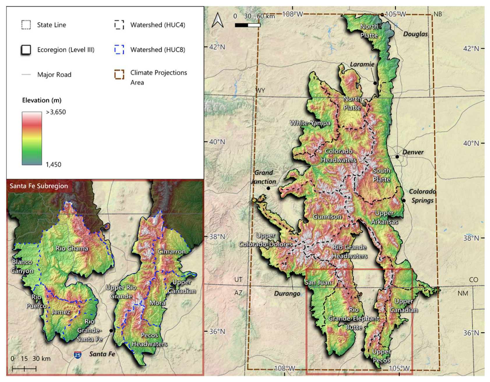
Figure 2.
Surface ownership distribution across the Southern Rocky Mountains Ecoregion and Santa Fe Subregion, Wyoming to New Mexico.
Figure 2.
Surface ownership distribution across the Southern Rocky Mountains Ecoregion and Santa Fe Subregion, Wyoming to New Mexico.
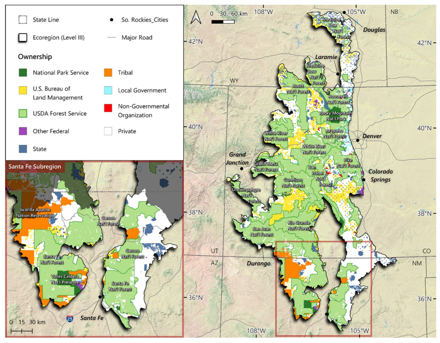
Figure 3.
Wolverine connectivity scores for the Southern Rockies Ecoregion and Santa Fe Subregion based on Carroll et al. [26]. Note the clustering of dark colors that may act as important linkage zones for connectivity and dispersal of wolverine across the ecoregion.
Figure 3.
Wolverine connectivity scores for the Southern Rockies Ecoregion and Santa Fe Subregion based on Carroll et al. [26]. Note the clustering of dark colors that may act as important linkage zones for connectivity and dispersal of wolverine across the ecoregion.
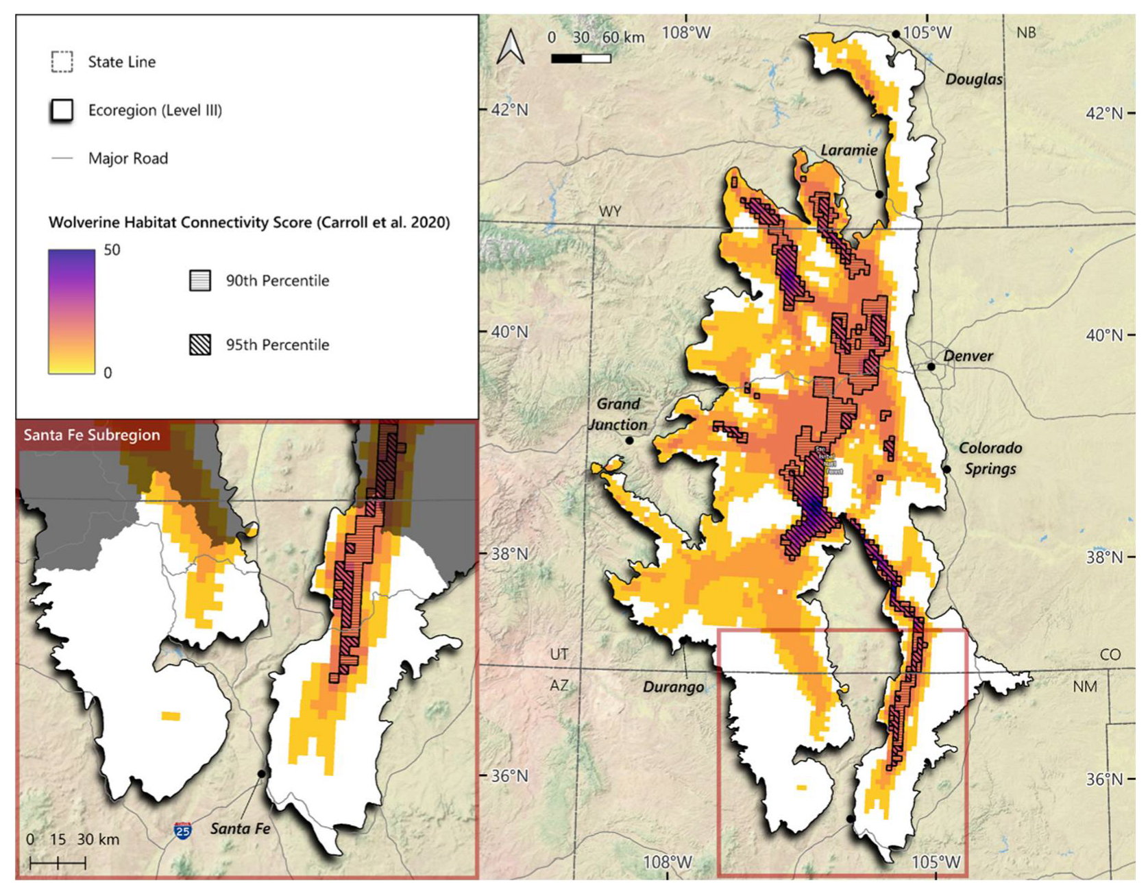
Figure 4.
Suitable habitat for both the Mexican Spotted Owl and Northern Goshawk in the Southern Rocky Mountains Ecoregion and Santa Fe Subregion.
Figure 4.
Suitable habitat for both the Mexican Spotted Owl and Northern Goshawk in the Southern Rocky Mountains Ecoregion and Santa Fe Subregion.

Figure 5.
Wildfires within the Southern Rocky Mountains Ecoregion and Santa Fe Subregion (1984-2022) in the Wildland Urban Interface, Wilderness, and Inventoried Roadless Areas.
Figure 5.
Wildfires within the Southern Rocky Mountains Ecoregion and Santa Fe Subregion (1984-2022) in the Wildland Urban Interface, Wilderness, and Inventoried Roadless Areas.
Figure 6.
Mean temperature across the study area from 1950 to 2100 under the lower (blue) and higher (pink) emissions scenarios. Graph created with Climate Toolbox Future Time Series web tool [37].
Figure 6.
Mean temperature across the study area from 1950 to 2100 under the lower (blue) and higher (pink) emissions scenarios. Graph created with Climate Toolbox Future Time Series web tool [37].
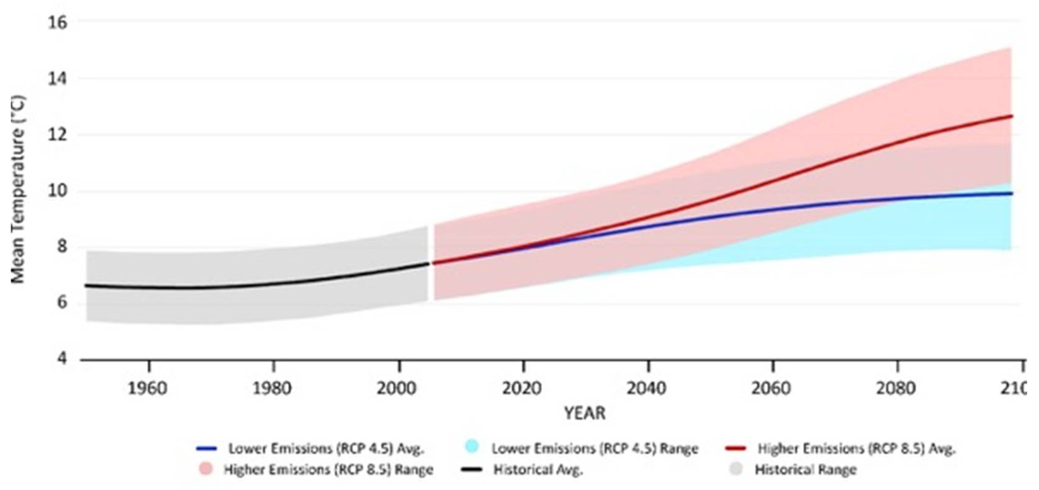
Figure 7.
Projected streamflow (m3/s) on the Colorado River at the Glenwood Springs Gauge Station from 2070-2099, as compared to historical flows (1950-2005). Historical flows (dark blue) show a peak in June and lowest flows during winter, while future flows are expected to peak in April/May and be lower during summer months. The high emissions scenario (RCP8.5, orange) leads to lower summer flows and a higher spring peak than the low emissions scenario (RCP 4.5, light blue). Graphic downloaded from Climate Toolbox Future Streamflow web tool based on VIC-MACAv2-Livneh CMIP5 multi-model mean bias-corrected data [37].
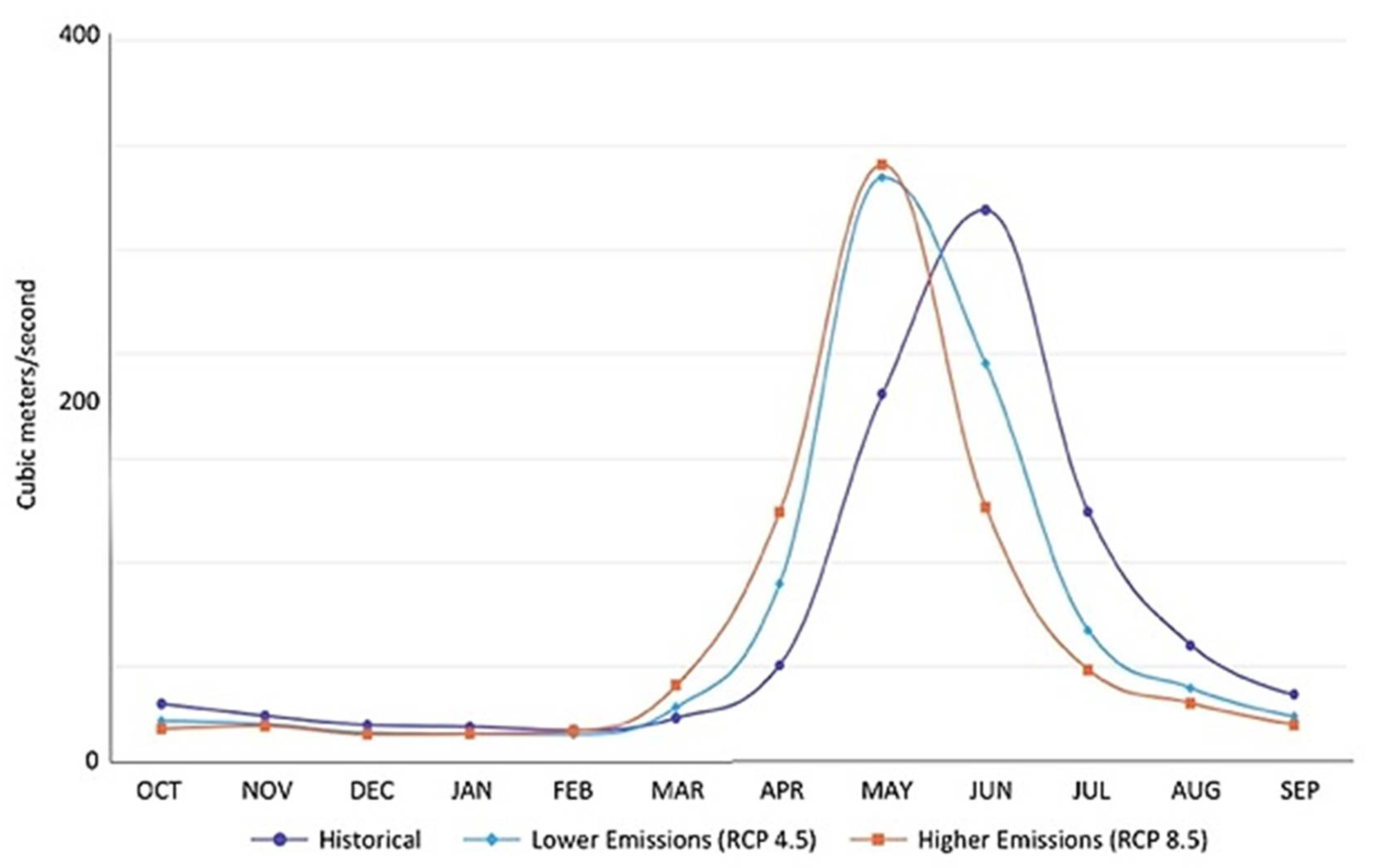

Table 1.
Landownerships and GAP status for the Southern Rocky Mountain Ecoregion.
| Southern Rocky Mountains Ecoregion | ||||||
|---|---|---|---|---|---|---|
| Owner Category | GAP ha | Total Owner Category ha |
||||
| (%) | ||||||
| 1 | 2 | 2.5 | 3 | 4 | (%) | |
| National Park Service | 139,643 | 40,539 | 1 | 8,684 | 4,302 | 193,170 |
| (72.3) | (21.0) | (0.0) | (4.5) | (2.2) | (1.3) | |
| U.S. Bureau of Land Management | 20,911 | 104,967 | 143 | 1,059,753 | 7,847 | 1,193,622 |
| (1.8) | (8.8) | (0.0) | (88.8) | (0.7) | (8.2) | |
| USDA Forest Service | 1,486,778 | 510,940 | 1,396,938 | 3,614,900 | 9,478 | 7,019,033 |
| (21.2) | (7.3) | (19.9) | (51.5) | (0.1) | (48.5) | |
| Other Federal1 | 20 | 10,866 | 0 | 497 | 39,025 | 50,408 |
| (0.0) | (21.6) | (0.0) | (1.0) | (77.4) | (0.3) | |
| State | 79 | 52,332 | 353 | 303,385 | 202,997 | 559,145 |
| (0.0) | (9.4) | (0.1) | (54.3) | (36.3) | (3.9) | |
| Local Government | 1,284 | 24,838 | 43 | 8,924 | 52,801 | 87,889 |
| (1.5) | (28.3) | (0.0) | (10.2) | (60.1) | (0.6) | |
| Tribal | 1 | 274 | 64 | 174 | 413,551 | 414,064 |
| (0.0) | (0.1) | (0.0) | (0.0) | (99.9) | (2.9) | |
| Non-Governmental Organization |
128 | 22,579 | 10 | 2,263 | 7,185 | 32,165 |
| (0.4) | (70.2) | (0.0) | (7.0) | (22.3) | (0.2) | |
| Private | 2,326 | 209,099 | 2,174 | 108,796 | 4,603,628 | 4,926,023 |
| (0.0) | (4.2) | (0.0) | (2.2) | (93.5) | (34.0) | |
| Total GAP ha | 1,651,170 | 976,433 | 1,399,726 | 5,107,376 | 5,340,813 | 14,475,519 |
| (%) | (11.4) | (6.7) | (9.7) | (35.3) | (36.9) | |
1 Includes U.S. Army Corps of Engineers, U.S. Bureau of Reclamation, U.S. Department of Agriculture (non-Forest Service), U.S. Department of Defense, U.S. Department of Energy, U.S. Department of Interior (non-Bureau of Land Management, non-National Park Service, non-Fish and Wildlife Service), and U.S. Fish and Wildlife Service.
Table 2.
Landownerships and GAP status for the Santa Fe Subregion.
| Southern Rocky Mountains Ecoregion | ||||||
|---|---|---|---|---|---|---|
| Owner Category | GAP ha | Total Owner Category ha |
||||
| (%) | ||||||
| 1 | 2 | 2.5 | 3 | 4 | (%) | |
| National Park Service | 12,605 | 38,609 | 0 | 0 | 0 | 51,214 |
| (24.6) | (75.4) | (0.0) | (0.0) | (0.0) | (2.3) | |
| U.S. Bureau of Land Management | 0 | 0 | 0 | 0 | 0 | 0 |
| (0.0) | (0.0) | (0.0) | (0.0) | (0.0) | (0.0) | |
| USDA Forest Service | 162,852 | 10,581 | 99,897 | 740,343 | 36 | 1,013,710 |
| (16.1) | (1.0) | (9.9) | (73.0) | (0.0) | (46.3) | |
| Other Federal 1 | 1 | 8,003 | 2 | 41,924 | 10,287 | 60,217 |
| (0.0) | (13.3) | (0.0) | (69.6) | (17.1) | (2.8) | |
| State | 0 | 31,818 | 1 | 8,781 | 30,634 | 71,234 |
| (0.0) | (44.7) | (0.0) | (12.3) | (43.0) | (3.3) | |
| Local Government | 0 | 2 | 1 | 0 | 893 | 897 |
| (0.0) | (0.3) | (0.1) | (0.0) | (99.6) | (0.0) | |
| Tribal | 1 | 274 | 64 | 45 | 264,245 | 264,630 |
| (0.0) | (0.1) | (0.0) | (0.0) | (99.9) | (12.1) | |
| Non-Governmental Organization |
0 | 215 | 0 | 0 | 0 | 215 |
| (0.0) | (100.0) | (0.0) | (0.0) | (0.0) | (0.0) | |
| Private | 86 | 1,272 | 380 | 7,311 | 716,884 | 725,933 |
| (0.0) | (0.2) | (0.1) | (1.0) | (98.8) | (33.2) | |
| Total GAP ha | 175,546 | 90,775 | 100,345 | 798,404 | 1,022,980 | 2,188,050 |
| (%) | (8.0) | (4.1) | (4.6) | (36.5) | (46.8) | |
1 Includes U.S. Army Corps of Engineers, U.S. Bureau of Reclamation, U.S. Department of Agriculture (non-Forest Service), U.S. Department of Defense, U.S. Department of Energy, U.S. Department of Interior (non-Bureau of Land Management, non-National Park Service, non-Fish and Wildlife Service), and U.S. Fish and Wildlife Service.
Table 3.
GAP status of Existing Vegetation Type categories (see Table S2 for definition of categories) for the Southern Rocky Mountain Ecoregion.
Table 3.
GAP status of Existing Vegetation Type categories (see Table S2 for definition of categories) for the Southern Rocky Mountain Ecoregion.
| Southern Rocky Mountains Ecoregion | ||||||
|---|---|---|---|---|---|---|
| Existing Vegetation Type (EVT) Category | GAP ha | Total EVT Category ha | ||||
| (%) | ||||||
| 1 | 2 | 2.5 | 3 | 4 | (%) | |
| Agricultural | 269 | 11,263 | 1,008 | 22,927 | 221,516 | 256,983 |
| (0.1) | (4.4) | (0.4) | (8.9) | (86.2) | (1.8) | |
| Alpine | 90,446 | 29,059 | 22,827 | 29,109 | 9,781 | 181,223 |
| (49.9) | (16.0) | (12.6) | (16.1) | (5.4) | (1.3) | |
| Aspen and Mixed-Conifer Forest | 5,177 | 2,484 | 17,949 | 33,109 | 9,966 | 68,684 |
| (7.5) | (3.6) | (26.1) | (48.2) | (14.5) | (0.5) | |
| Aspen Forest and Woodland | 107,598 | 92,004 | 236,841 | 500,609 | 343,511 | 1,280,563 |
| (8.4) | (7.2) | (18.5) | (39.1) | (26.8) | (8.8) | |
| Barren | 52,872 | 13,289 | 18,192 | 26,440 | 22,601 | 133,395 |
| (39.6) | (10.0) | (13.6) | (19.8) | (16.9) | (0.9) | |
| Developed | 1,443 | 4,819 | 541 | 42,593 | 167,541 | 216,938 |
| (0.7) | (2.2) | (0.2) | (19.6) | (77.2) | (1.5) | |
| Grassland | 80,727 | 95,578 | 71,477 | 386,897 | 807,428 | 1,442,106 |
| (5.6) | (6.6) | (5.0) | (26.8) | (56.0) | (10.0) | |
| Limber Pine Woodland | 4 | 237 | 26 | 2,165 | 1,489 | 3,921 |
| (0.1) | (6.1) | (0.7) | (55.2) | (38.0) | (0.0) | |
| Lodgepole Pine Forest | 114,905 | 64,508 | 137,148 | 408,600 | 106,138 | 831,299 |
| (13.8) | (7.8) | (16.5) | (49.2) | (12.8) | (5.7) | |
| Mixed-Conifer Forest | 91,210 | 87,846 | 154,977 | 506,968 | 362,187 | 1,203,189 |
| (7.6) | (7.3) | (12.9) | (42.1) | (30.1) | (8.3) | |
| Pinyon-Juniper | 18,355 | 50,682 | 36,605 | 386,388 | 463,682 | 955,712 |
| (1.9) | (5.3) | (3.8) | (40.4) | (48.5) | (6.6) | |
| Ponderosa Pine | 35,994 | 83,489 | 112,688 | 842,012 | 1,130,986 | 2,205,170 |
| (1.6) | (3.8) | (5.1) | (38.2) | (51.3) | (15.2) | |
| Riparian | 21,052 | 13,503 | 17,583 | 80,563 | 113,188 | 245,889 |
| (8.6) | (5.5) | (7.2) | (32.8) | (46.0) | (1.7) | |
| Shrubland | 67,705 | 127,211 | 118,569 | 904,887 | 1,250,583 | 2,468,954 |
| (2.7) | (5.2) | (4.8) | (36.7) | (50.7) | (17.1) | |
| Snow-Ice | 41,221 | 8,151 | 2,358 | 7,225 | 2,348 | 61,304 |
| (67.2) | (13.3) | (3.8) | (11.8) | (3.8) | (0.4) | |
| Sparse | 162,830 | 35,553 | 39,627 | 43,009 | 16,005 | 297,024 |
| (54.8) | (12.0) | (13.3) | (14.5) | (5.4) | (2.1) | |
| Subalpine Forest | 747,527 | 240,071 | 405,574 | 836,305 | 211,538 | 2,441,016 |
| (30.6) | (9.8) | (16.6) | (34.3) | (8.7) | (16.9) | |
| Water | 3,725 | 5,335 | 1,698 | 21,600 | 30,441 | 62,799 |
| (5.9) | (8.5) | (2.7) | (34.4) | (48.5) | (0.4) | |
| Wetland | 8,111 | 11,349 | 4,037 | 25,971 | 69,883 | 119,351 |
| (6.8) | (9.5) | (3.4) | (21.8) | (58.6) | (0.8) | |
| Total GAP ha | 1,651,170 | 976,433 | 1,399,726 | 5,107,376 | 5,340,813 |
14,475,519 (100%) |
| (%) | (11.4) | (6.7) | (9.7) | (35.3) | (36.9) | |
Table 4.
GAP status of Existing Vegetation Type categories (see Table S2 for definition of categories) for the Santa Fe Subregion.
Table 4.
GAP status of Existing Vegetation Type categories (see Table S2 for definition of categories) for the Santa Fe Subregion.
| Santa Fe Subregion | ||||||
|---|---|---|---|---|---|---|
| Existing Vegetation Type (EVT) Category | GAP ha | Total EVT Category ha | ||||
| (%) | ||||||
| 1 | 2 | 2.5 | 3 | 4 | (%) | |
| Agricultural | 40 | 455 | 101 | 1,833 | 27,075 | 29,505 |
| (0.1) | (1.5) | (0.3) | (6.2) | (91.8) | (1.3) | |
| Alpine | 453 | 141 | 25 | 182 | 1,208 | 2,009 |
| (22.6) | (7.0) | (1.2) | (9.1) | (60.1) | (0.1) | |
| Aspen and Mixed-Conifer Forest | 306 | 371 | 172 | 890 | 2,136 | 3,875 |
| (7.9) | (9.6) | (4.4) | (23.0) | (55.1) | (0.2) | |
| Aspen Forest and Woodland | 9,814 | 4,648 | 3,495 | 30,877 | 28,563 | 77,397 |
| (12.7) | (6.0) | (4.5) | (39.9) | (36.9) | (3.5) | |
| Barren | 4,045 | 438 | 290 | 799 | 3,185 | 8,757 |
| (46.2) | (5.0) | (3.3) | (9.1) | (36.4) | (0.4) | |
| Developed | 223 | 668 | 97 | 4,544 | 21,545 | 27,077 |
| (0.8) | (2.5) | (0.4) | (16.8) | (79.6) | (1.2) | |
| Grassland | 6,756 | 11,666 | 4,544 | 30,197 | 67,543 | 120,706 |
| (5.6) | (9.7) | (3.8) | (25.0) | (56.0) | (5.5) | |
| Limber Pine Woodland | 0 | 0 | 0 | 0 | 0 | 0 |
| (0.0) | (0.0) | (0.0) | (0.0) | (0.0) | (0.0) | |
| Lodgepole Pine Forest | 0.1 | 1 | 1 | 0.1 | 0 | 2 |
| (4.3) | (39.1) | (52.2) | (4.3) | (0.0) | (0.0) | |
| Mixed-Conifer Forest | 40,613 | 20,745 | 26,675 | 159,960 | 113,726 | 361,719 |
| (11.2) | (5.7) | (7.4) | (44.2) | (31.4) | (16.5) | |
| Pinyon-Juniper | 13,342 | 8,390 | 20,138 | 145,166 | 196,042 | 383,078 |
| (3.5) | (2.2) | (5.3) | (37.9) | (51.2) | (17.5) | |
| Ponderosa Pine | 16,241 | 17,185 | 21,711 | 298,328 | 308,192 | 661,657 |
| (2.5) | (2.6) | (3.3) | (45.1) | (46.6) | (30.2) | |
| Riparian | 948 | 1,146 | 495 | 4,920 | 12,284 | 19,793 |
| (4.8) | (5.8) | (2.5) | (24.9) | (62.1) | (0.9) | |
| Shrubland | 15,066 | 13,315 | 10,137 | 64,256 | 155,022 | 257,795 |
| (5.8) | (5.2) | (3.9) | (24.9) | (60.1) | (11.8) | |
| Snow-Ice | 9 | 0 | 0 | 0 | 12 | 21 |
| (43.9) | (0.0) | (0.0) | (0.0) | (56.1) | (0.0) | |
| Sparse | 1,206 | 146 | 271 | 650 | 1,122 | 3,395 |
| (35.5) | (4.3) | (8.0) | (19.1) | (33.1) | (0.2) | |
| Subalpine Forest | 66,104 | 8,037 | 12,129 | 53,830 | 72,629 | 212,730 |
| (31.1) | (3.8) | (5.7) | (25.3) | (34.1) | (9.7) | |
| Water | 91 | 351 | 3 | 118 | 4,298 | 4,860 |
| (1.9) | (7.2) | (0.1) | (2.4) | (88.4) | (0.2) | |
| Wetland | 289 | 3,072 | 60 | 1,855 | 8,397 | 13,673 |
| (2.1) | (22.5) | (0.4) | (13.6) | (61.4) | (0.6) | |
| Total GAP ha | 175,546 | 90,775 | 100,345 | 798,404 | 1,022,980 |
2,188,050 (100.0) |
| (%) | (8.0) | (4.1) | (4.6) | (36.5) | (46.8) | |
Table 5.
Forest structure classes (based on [25]) and GAP status within the Southern Rocky Mountain Ecoregion and Santa Fe Subregion.
Table 5.
Forest structure classes (based on [25]) and GAP status within the Southern Rocky Mountain Ecoregion and Santa Fe Subregion.
| Southern Rocky Mountains Ecoregion | ||||||
|---|---|---|---|---|---|---|
| Forest Structure Class | GAP ha | Total Forest Structure Class ha | ||||
| (%) | ||||||
| 1 | 2 | 2.5 | 3 | 4 | (%) | |
| Young | 214,080 | 110,619 | 189,426 | 618,906 | 381,940 | 1,514,970 |
| (14.1) | (7.3) | (12.5) | (40.9) | (25.2) | (22.9) | |
| Intermediate | 274,961 | 160,632 | 302,829 | 967,726 | 625,263 | 2,331,411 |
| (11.8) | (6.9) | (13.0) | (41.5) | (26.8) | (35.3) | |
| Mature | 387,317 | 206,024 | 438,769 | 1,078,196 | 650,641 | 2,760,947 |
| (14.0) | (7.5) | (15.9) | (39.1) | (23.6) | (41.8) | |
| Total GAP ha | 876,358 | 477,275 | 931,024 | 2,664,829 | 1,657,843 |
6,607,329 (100.0) |
| (13.3) | (7.2) | (14.1) | (40.3) | (25.1) | ||
| Santa Fe Subregion | ||||||
| Forest Structure Class | GAP ha | Total Forest Structure Class ha | ||||
| (%) | ||||||
| 1 | 2 | 2.5 | 3 | 4 | (%) | |
| Young | 16,957 | 10,126 | 9,021 | 78,272 | 78,996 | 193,372 |
| (8.8) | (5.2) | (4.7) | (40.5) | (40.9) | (15.9) | |
| Intermediate | 33,504 | 18,373 | 19,557 | 182,556 | 167,959 | 421,949 |
| (7.9) | (4.4) | (4.6) | (43.3) | (39.8) | (34.7) | |
| Mature | 74,385 | 22,007 | 41,420 | 275,932 | 187,588 | 601,332 |
| (12.4) | (3.7) | (6.9) | (45.9) | (31.2) | (49.4) | |
| Total GAP ha | 124,846 | 50,505 | 69,999 | 536,760 | 434,542 |
1,216,653 (100.0) |
| (10.3) | (4.2) | (5.8) | (44.1) | (35.7) | ||
Table 6.
GAP status of upper tiers of wolverine habitat connectivity across the Southern Rocky Mountains Ecoregion and Santa Fe Subregion.
Table 6.
GAP status of upper tiers of wolverine habitat connectivity across the Southern Rocky Mountains Ecoregion and Santa Fe Subregion.
| Southern Rocky Mountains Ecoregion | ||||||
|---|---|---|---|---|---|---|
| Wolverine Habitat Connectivity Tier | GAP ha | Wolverine Habitat Connectivity Tier ha | ||||
| (%) | ||||||
| 1 | 2 | 2.5 | 3 | 4 | (%) | |
| 90th Percentile | 370,568 | 142,632 | 259,856 | 565,749 | 255,199 | 1,594,004 |
| (23.2) | (8.9) | (16.3) | (35.5) | (16.0) | (66.7) | |
| 95th Percentile | 186,999 | 59,476 | 145,152 | 299,470 | 104,002 | 795,099 |
| (23.5) | (7.5) | (18.3) | (37.7) | (13.1) | (33.3) | |
| Total GAP ha | 557,567 | 202,108 | 405,008 | 865,219 | 359,201 | 2,389,103 |
| (23.3) | (8.5) | (17.0) | (36.2) | (15.0) | ||
| Santa Fe Subregion | ||||||
| Wolverine Habitat Connectivity Tier | GAP ha | Wolverine Habitat Connectivity Tier ha | ||||
| (%) | ||||||
| 1 | 2 | 2.5 | 3 | 4 | (%) | |
| 90th Percentile | 16,567 | 4 | 2,224 | 45,033 | 49,005 | 112,833 |
| (14.7) | (0.0) | (2.0) | (39.9) | (43.4) | (73.9) | |
| 95th Percentile | 10,559 | 2 | 809 | 13,624 | 14,807 | 39,801 |
| (26.5) | (0.0) | (2.0) | (34.2) | (37.2) | (26.1) | |
| Total GAP ha | 27,126 | 6 | 3,033 | 58,657 | 63,812 | 152,634 |
| (17.8) | (0.0) | (2.0) | (38.4) | (41.8) | ||
Table 7.
Suitable habitat for Mexican spotted owl, northern goshawk, and Canada lynx along with their GAP status within the Southern Rocky Mountain Ecoregion and Santa Fe Subregion.
Table 7.
Suitable habitat for Mexican spotted owl, northern goshawk, and Canada lynx along with their GAP status within the Southern Rocky Mountain Ecoregion and Santa Fe Subregion.
| Southern Rocky Mountains Ecoregion | ||||||
|---|---|---|---|---|---|---|
| Focal Species | GAP ha | Total Focal Species Suitable Habitat ha | ||||
| (%) | ||||||
| 1 | 2 | 2.5 | 3 | 4 | (%) | |
| Mexican Spotted Owl | 7,912 | 17,767 | 32,989 | 181,424 | 104,697 | 344,789 |
| (2.3) | (5.2) | (9.6) | (52.6) | (30.4) | (2.7) | |
| Northern Goshawk | 995,417 | 637,456 | 1,041,847 | 3,732,433 | 3,299,723 | 9,706,876 |
| (10.3) | (6.6) | (10.7) | (38.5) | (34.0) | (75.2) | |
| Canada Lynx | 558,604 | 258,103 | 520,036 | 1,163,796 | 356,529 | 2,857,068 |
| (19.6) | (9.0) | (18.2) | (40.7) | (12.5) | (22.1) | |
| Total GAP ha | 1,561,934 | 913,326 | 1,594,872 | 5,077,653 | 3,760,949 | 12,908,733 |
| (12.1) | (7.1) | (12.4) | (39.3) | (29.1) | ||
| Santa Fe Subregion | ||||||
| Focal Species | GAP ha | Total Focal Species Suitable Habitat ha | ||||
| (%) | ||||||
| 1 | 2 | 2.5 | 3 | 4 | (%) | |
| Mexican Spotted Owl | 7,218 | 4,054 | 11,312 | 112,238 | 58,596 | 193,419 |
| (3.7) | (2.1) | (5.8) | (58.0) | (30.3) | (9.9) | |
| Northern Goshawk | 130,313 | 65,243 | 83,743 | 684,744 | 800,875 | 1,764,918 |
| (7.4) | (3.7) | (4.7) | (38.8) | (45.4) | (90.1) | |
| Canada Lynx | 0 | 0 | 0 | 0 | 0 | 0 |
| (0.0) | (0.0) | (0.0) | (0.0) | (0.0) | (0.0) | |
| Total GAP ha | 137,531 | 69,297 | 95,056 | 796,982 | 859,471 | 1,958,337 |
| (7.0) | (3.5) | (4.9) | (40.7) | (43.9) | ||
Table 8.
Wildland-Urban interface/intermix class distribution across the SRME and SFSR and the relative proportions that were intersected by at least one fire between 1984 and 2022.
Table 8.
Wildland-Urban interface/intermix class distribution across the SRME and SFSR and the relative proportions that were intersected by at least one fire between 1984 and 2022.
| Wildland-Urban Interface/Intermix (2020) Class | Southern Rocky Mountains Ecoregion | Santa Fe Subregion | ||
|---|---|---|---|---|
| All ha | Burned ha | All ha | Burned ha | |
| (%) | (%) | (%) | (%) | |
| Low Density Intermix | 410,361 | 25,685 | 51,441 | 4,909 |
| (75.6) | (88.5) | (77.0) | (90.9) | |
| Medium Density Intermix | 69,114 | 1,442 | 7,392 | 166 |
| (12.7) | (5.0) | (11.1) | (3.1) | |
| High Density Intermix | 237 | 2 | 26 | 1 |
| (0.0) | (0.0) | (0.0) | (0.0) | |
| Low Density Interface | 25,640 | 1,536 | 5,086 | 165 |
| (4.7) | (5.3) | (7.6) | (3.1) | |
| Medium Density Interface | 31,149 | 295 | 2,495 | 113 |
| (5.7) | (1.0) | (3.7) | (2.1) | |
| High Density Interface | 6,097 | 78 | 357 | 48 |
| (1.1) | (0.3) | (0.5) | (0.9) | |
| Total ha | 542,599 | 29,037 | 66,797 | 5,402 |
| (%)1 | (3.8) | (2.3) | (3.1) | (1.5) |
1The first and third columns are the percentages of the SRME and SFSR, respectively. The second and fourth columns are the percentages of the total burned area within the SRME (1,270,603 ha) and SFSR (366,839 ha), respectively.
Table 9.
Historical (1979-2023) climate changes for the Southern Rocky Mountains Ecoregion.1.
| Average Annual Temperature | +1.2°C |
| Maximum Temperature | +0.8°C |
| Minimum Temperature | +1.5°C |
| Frost Free Days | +29 days longer frost-free season |
| Annual Precipitation | -15% |
| Drought2 | Increasing frequency |
| Snowpack3 | <20% at most sites |
1GridMET gridded surface meteorological dataset accessed from Climatetoolbox.org; April 4, 2024. 2Palmer Drought Severity Index (PDSI) accessed from Climatetoolbox.org. 3EPA 2023. https://www.epa.gov/climate-indicators/climate-change-indicators-snowpack; accessed May 10, 2024.
Table 10.
Estimated number of additional days per year over 32°C, 38°C, and 41°C across the Southern Rocky Mountain Ecoregion based on continued high emissions (RCP8.5) vs. low emissions (RCP4.5) scenarios for two time periods (2040-69, 2070-99). Data accessed from Climate Toolbox Future Box Plots web tool [37].
| Years | RCP8.5 | RCP4.5 | ||||
|---|---|---|---|---|---|---|
| > 32°C | > 38°C | > 41°C | > 32°C | > 38°C | > 41°C | |
| 2040-69 | +19.6 | +1.3 | +0.1 | +12.3 | +0.4 | +0.0 |
| 2070-99 | +39.3 | +6.4 | +1.1 | +15.2 | +0.7 | +0.0 |
Disclaimer/Publisher’s Note: The statements, opinions and data contained in all publications are solely those of the individual author(s) and contributor(s) and not of MDPI and/or the editor(s). MDPI and/or the editor(s) disclaim responsibility for any injury to people or property resulting from any ideas, methods, instructions or products referred to in the content. |
© 2024 by the authors. Licensee MDPI, Basel, Switzerland. This article is an open access article distributed under the terms and conditions of the Creative Commons Attribution (CC BY) license (http://creativecommons.org/licenses/by/4.0/).
Copyright: This open access article is published under a Creative Commons CC BY 4.0 license, which permit the free download, distribution, and reuse, provided that the author and preprint are cited in any reuse.


