Submitted:
23 July 2024
Posted:
25 July 2024
You are already at the latest version
Abstract
This paper presents a methodology based on deep learning models and metaheuristic algorithms for the optimization of airfoils for the design of aircraft wings with large endurance. The use of AZTLI-NN (a neural network with an architecture composed of a multilayer perceptron and a variational autoencoder) is implemented for the prediction of graphs of the aerodynamic coefficients of the airfoil as a function of the angle of attack. This neural network presents good predictions of the aerodynamic coefficients, similar to the coefficients obtained with computational fluid dynamics simulations. AZTLI-NN in combination of metaheuristic algorithms and the CST profile parameterization method show excellent performance in single-objective and multi-objective profile optimization tasks.
Keywords:
airfoil optimization
; OpenFOAM
; deep learning models
; metaheuristics algorithms
; method CST
1. Introduction
As a key component of aircraft, an excellent aerodynamic configuration of the airfoil plays a crucial role in fuel economy, reducing polluting emissions and improving performance [1,2,3]. In the design of unmanned aerial vehicles (UAV) and gliders, the development of wing configurations with a high aspect ratio is also being opted for, because these wing configurations provide a better range and flight duration. In UAVs there is a greater interest in improving the flight duration, especially in subsonic flight missions, in missions such as: reconnaissance, target tracking, pseudo-satellites, etc [4].
Taking into account the aircraft powered by propeller engines, aerodynamically, an aircraft to achieve a large endurance its CL1.5/CD (CL, lift coefficient; CD, drag coefficient) ratio values should be the highest possible [5]. This CL1.5/CD ratio is usually called the endurance parameter. As mentioned above, this is mainly achieved by having a wing with a high aspect ratio, but the shape of the airfoils along the wingspan is also of utmost importance, which should also provide a high cl1.5/cd value [4,6]. The design of this type of airfoils is obtained by optimizing the shape of the airfoil, which must produce a high value of the endurance parameter with respect to a design lift coefficient. It is important to mention that airfoils with high values of cl1.5/cd and cl usually have convex shapes that generate very negative values of pitch moment coefficient (cm). This drawback is compensated by the empennage of the aircraft. Although in aircraft configurations that lack a horizontal empennage (such as flying wings) it is necessary that the cm be as close to zero, for this reason in these cases an extra objective function is usually added to the optimization task, minimizing |cm| [4,7].
Computational fluid dynamics (CFD), wind tunnel testing and theoretical analysis have gradually become the main approaches to aerodynamic design, advancing the progress of aerodynamic optimization of airfoils. However, in real engineering design, wind tunnel tests are expensive, and theoretical analysis is less applicable when dealing with complex engineering problems, so CFD has gradually become the main method for aerodynamic analysis [8].
The basic element of aerodynamic optimization of the airfoil mainly includes the design object, the design objective, the design constraints and the design method (optimization method). Design object refers to the aerodynamic geometric configuration. The design objective refers to the expected aerodynamic performance, the characteristics of the flow field, etc. The design constraints illustrate the interdependence and constraints between the design variables of the design object. And optimization methods provide the strategies and means to achieve the design goal [8].
Currently there are a large number of optimization methods that are widely used. These methods can be generally classified into gradient-based and gradient-free optimization methods. Current gradient-based approaches use discrete adjunct sensitivity analysis, scale approximately linearly with the number of design variables, and are very capable of handling thousands of design variables and constraints. The advantages of gradient-based optimization to address airfoil shape optimization are low computational costs in large design spaces and a track record of successful implementations in aerodynamics. However, there are some drawbacks to this approach, such as the tendency to converge on local optima and a high sensitivity to the starting point, poor efficiency for nonlinear cost functions and the need for continuous shapes (the shape gradient must exist at all points). The gradient-based approach may be more appropriate for a detailed aerodynamic design, as they are only able to offer a limited range of solutions. Gradient-free methods can be more complex to implement than gradient-based methods, but they do not require continuity or predictability in the design space and usually increase the probability of finding a global optimum. Optimization methods known as metaheuristics can offer robust methods for finding a solution and increase the probability of converging on a solution at the global optimum. It is known that these gradient-free methods are able to address numerically noisy optimization problems that are difficult for gradient-based methods. And unlike gradient methods, derivatives of cost functions are not necessary. In addition, no predefined baseline design or knowledge of the design space is required and gradient-free methods usually optimize several solutions in parallel. However, their convergence speeds are usually slow enough that they are unable to cooperate directly with time-consuming CFD analysis. To counteract this disadvantage that metaheuristic methods have, in the first instance, more robust computing equipment is used (which implies raising the costs of the optimization process). Another alternative is to make use of methods based on surrogate models [8,9,10,11].
Traditional methods for training surrogate models include the polynomial response surface method, the support vector regression method, and the Kriging model. The traditional substitute model has adjustable parameters; however, the main problem is that it is not suitable for handling large-scale training data, so it is usually trained with a small amount of data in a relatively limited space [8,9,10,11,12]. Recent advances in machine learning (especially in deep learning methods: artificial neural networks) have provided a new option for generating surrogate models. Compared to traditional surrogate models, the advantages of applying neural networks in aerodynamic data modeling lie in the fact that: a) neural networks, as a data-driven model, are not based on aerodynamic theories or physical models, which means that it does not require in-depth knowledge of aerodynamics; b) neural networks can be used to address high-dimensional, multi-scale and nonlinear problems that are difficult for traditional surrogate models; and c) some neural networks have the ability to process time sequence data [13].
In the present work, a methodology is developed to accelerate the process of airfoil optimization under conditions of subsonic, incompressible and turbulent flow, making use of current deep learning models and metaheuristic algorithms. This research work is specifically aimed at the design of aircraft with long endurance operating in subsonic flight regime.
2. Materials and Methods
2.1. Mathematical Formulation of the Problems
Two cases are considered:
- determination of the airfoil shape producing a long endurance parameter (cl1.5/cd) with respect to a specified lift coefficient;
- determination of the airfoil shape producing a long endurance parameter (cl1.5/cd) and a near-zero value of the pitch moment coefficient (cm) with respect to a specified lift coefficient.
The purpose of the above cases is to contemplate aircraft configurations with empennage and without empennage.
For the first case, it is only necessary to maximize the endurance parameter and consider design constraints such as the design lift coefficient.
max f1(ξ) = cl1.5/cd,
such that ha(ξ) = 0, a = 1, 2, ..., A,
gb(ξ) ≤ 0, b = 1, 2, ..., B,
ξ ∊ Ω.
For the second case, the objective of minimizing the magnitude of cm is added.
where ξ is the vector of design parameters; h(ξ) are constraint functions (equalities); g(ξ) are constraint functions(inequalities); Ω is the decision space of the design parameters.
max f1(ξ) = cl1.5/cd,
min f2(ξ) = |cm|
such that ha(ξ) = 0, a = 1, 2, ..., A,
gb(ξ) ≤ 0, b = 1, 2, ..., B,
ξ ∊ Ω.
To provide a solution to the above optimization tasks, the following methodology is proposed:
- Selecting a method of parameterization of the aerodynamic profile, the method should allow modeling aerodynamic profiles used for the design of aircraft with long-span wings;
- Select a robust method that allows the aerodynamic coefficients of the airfoils to be calculated. The method should take into account the viscosity and turbulence effects of the flow;
- Propose a model based on deep learning models to predict the values of the objective functions, this in order to speed up the process of calculating the objective functions;
- Finally, select the appropriate optimization algorithms for each task.
2.2. Selection of the Method of Airfoils Parameterization
To determine the design parameters, two of the best airfoil parameterization methods were evaluated: CST (see Appendix A) and Bezier-PARSEC (see Appendix B) methods. The way to evaluate the methods is to evaluate the capabilities they have when reconstructing the geometry existing airfoils (such as NACA, Eppler, TSAGI, etc.). Obtaining the original coordinates of the airfoils is carried out using the profile database of the University of Illinois at Urbana-Champaign (UIUC) [14]. Only the selection of asymmetric airfoils that are used in general aviation (aircraft operating in subsonic and/or transonic flight regime) is contemplated [15].
The reconstruction of the airfoils is carried out through the use of the evolutionary algorithm Differential Evolution (DE), whose objective is to find the values of the design parameters of each method which provide the least geometric deviation when comparing the reconstructed profiles and the original ones [16]. The value of the geometric deviation is obtained by the error norm L2:
where ytar is the set of heights of the original points of the target profile; y is the set of heights of the reconstructed points; P is the number of points that make up the geometry of the airfoil.
2.3. Creation of a Database of Airfoils and Their Aerodynamic Coefficients
2.3.1. Geometries of the Airfoils
In the first instance, it is proposed to make use of the selected profiles from the UIUC database, in case these are not enough, the use of a Generative Adversarial Network (GAN) is suggested for the creation of new profiles, which will be based on the selected profiles from the UIUC database. GANs use a learning scheme that allows the defining attributes of the probability distribution to be encoded in a neural network, making it possible to generate instances that resemble the original probability distribution [17]. The GAN architecture is formed by two constituent neural networks: one called discriminator (D) and the other generator (G). The G network is responsible for generating new instances of the same domain as that of the source dataset. The network D is in charge of discriminating whether the input data are real, that is belonging to the input data set or whether they are fictitious, that is artificially generated. Both networks are trained together in such a way that G maximizes its chances of not being detected by D and D in such a way that it makes its methods of detecting the artificially generated data by G more and more sophisticated. These two adversarial networks compete in a zero-sum game in which it is hypothesized that they eventually reach a Nash equilibrium (see Figure 1) [18].
2.3.2. Obtaining the Aerodynamic Coefficients
The aerodynamic coefficients of the profiles are obtained by means of Computational Fluid Dynamics, using the CFD package OpenFOAM 11 [19] and the GMSH mesh generator [20]. It is considered a viscous, turbulent, steady and incompressible flow.
where ui is the average velocity; ν is the kinematic viscosity of the air; ρ is the density of the air; p is the pressure; u'iu'j is the Reynolds stress tensor.
To model the turbulence the k-ω SST model is considered. This is a two-equation turbulence model that is widely used to calculate the aerodynamic coefficients in subsonic and transonic flows. It combines the low Reynolds number version of the k-ω model and the high Reynolds number version of the k-ε model to obtain accurate results under a wide range of flow conditions. The k-ω SST model is computationally more expensive than other two-equation models, but can provide more accurate results for more complex flows [21,22,23]. OpenFOAM uses the version of the k-ω SST model exposed by Menter in [24]. The turbulence specific dissipation rate (ω) equation is given by:
and the kinetic energy of turbulence (k) is defined by:
where F1 is the blending function; S is the invariant measure of the strain rate; is a production limiter. All constants are computed by a blend from the corresponding constants of the k - ε and the k - ω models via α = α1F + α2(1 - F). The constants for this model are: β* = 0.09, α1 = 5/9, β = 3/40, σk1 = 0.85, σω1=0.5, α2 = 0.44, σω2 = 0.856 [24].
The k-ω SST model allows the use of wall functions, which allows the use of meshes that are not so thin next to the wall (y+ values between 10 and 100) without losing as much precision [24]. By having this tolerance in the y+ values, greater flexibility is possible when developing the mesh.
For the creation of the mesh, a control volume with a type C configuration [25] (see Figure 2(a)) and the use of hexahedral elements is considered (OpenFOAM does not work with two-dimensional meshes). Each mesh has 21360 hexahedral elements, which allows y+ values close to 10 when using turbulent flows with Re values between 1 million to 6 million (see Figure 2(b)). Most of the boundary conditions used are shown in Figure. 2(c) . The "wall" condition is applied to the faces that limit the geometry of the profile; the "outlet" condition is assigned to the vertical face located to the right of the control volume; the "inlet" condition is assigned to the arc faces and the upper and lower horizontal faces of the control volume; finally, the "empty" condition is applied to the front and rear faces of the control volume. This last condition is what indicates to OpenFOAM that the simulation is two-dimensional [19]. The entire control volume is defined as "internal field".
In the simulations, five physical fields are mainly evaluated: pressure (p) (in incompressible flow simulations, OpenFOAM, uses a specific pressure, p/ρ [19]), velocity (U), turbulent kinematic viscosity (νt), turbulent kinetic energy (k) and specific turbulence dispersion velocity (ω). Table 1 shows the initial conditions for each physical field at each boundary condition and for the internal field.
The values of ω and νt at the input, output and internal field are specified by default to work together with the wall function implemented on the profile wall [19,26]. The initial values of k are determined by the following equation [19]:
where I is the intensity of the turbulence and U∞ is the velocity of the free flow.
2.3.3. Encoding of the Data
When training neural networks, it is often useful to make sure that the data is normalized at all stages of the network. Normalization helps to stabilize and accelerate the training of the network by means of a downward gradient. If the data has been scaled badly, the loss function value may become an undefined value (NaN) and the network parameters may diverge during training. Common ways to normalize data include rescaling data so that its interval is [0, 1] or that it has a mean of zero and a standard deviation of one [27,28].
For normalization of the input vectors, which are the design parameters of the airfoils, the MinMax scaler is used [29], where the transformation is given by:
where ξj,min and ξj,max are the lower and upper limits of the calculated interval of the parameter ξj; dmin and dmax are new design intervals, 0 and 1, respectively.
For the case of the output data, the aerodynamic coefficients are represented in graphs, that is, images, which can be represented in matrices (three matrices representing the RGB layers), and whose components (pixels) have values between 0 and 1 (the original ranges are between 0 and 255, but the Python graphers also detect the range between 0 and 1 as valid) [30]. The graphs of interest are: endurance parameter vs angle of attack, pitch moment coefficient vs angle of attack and lift coefficient vs angle of attack. Each graph was normalized in images of 256 x 256 pixels, the axes and labels are eliminated, only the curve representing the values is left, the pixels that make up the curve have values of 1 (white color), while the pixels that make up the background have values of 0 (black color). Finally, the three images become layers of an RGB-encoded image (see Figure 3).
2.4. Design of the Neural Network for the Prediction of Aerodynamic Coefficients of Airfoils
The method for the design of the neural network is depicted in Figure 4, this method can be divided into the following three parts. 1 - the Principal Component Analysis (PCA) is used to perform the reduction of representative features of the output images and to obtain an approximation of the optimal dimension of the features involved in a Variational Autoencoder (VAE). 2 - VAE is used to extract representative features from the output images by unsupervised reconstruction-based learning. 3 - an Multi-layer Perceptron (MLP) network is developed to construct a non-linear mapping of the shapes of the aerodynamic surfaces to the features extracted by the VAE. The graphs of the aerodynamic coefficients of the profiles can be predicted by the composite network connecting the MLP and the decoder of the VAE [31].
2.4.1. Approximation of the Representative Features of the Output Images
The main goal of PCA is to find the principal component (PC) space, which is used to transform information from the original higher-dimensional space to the lower-dimensional space. The PC space consists of k components that are orthonormal, uncorrelated and represent the directions of the maximum variance of the data. The first principal component of the PCA space represents the direction of the maximum variance of the data, the second component has the second largest variance, and so on [32]. For image compression, the PCA method is used together with the information loss method (LOSSY). In the LOSSY method, some of the redundant information of the original file is lost, that is, when the file is restored, only the most important information is restored [29,32].
2.4.2. VAE Configuration
A VAE is a model consisting of an encoder and a decoder (see Figure 5). The encoder, also known as the output model or the recognition model, approximates the posterior distribution of the hidden variables of the decoder. The decoder is a deep hidden variable model and is a variation of the generative model. Both components, the encoder and the decoder, are directional graphic models that are totally or partially parameterized by deep neural networks [33].
In the case of an automatic encoder (AE), with a given input of ζ, the encoder converts ζ into a hidden representation of z that has a smaller dimension compared to ζ. The decoder then uses z to reconstruct ζ'. The recovery loss function L is calculated by comparing the differences between ζ and ζ'. VAEs are probabilistic modifications of AEs that combine Bayesian variational inference and deep learning. The encoder serves as an inference model that attempts to infer the latent variables z from the input data ζ through a learned distribution q(z|ζ); the decoder serves as a generative model that generates similar input data ζ‘ under the given latent vector z by sampling from learned distribution p(ζ|z). Assuming that the posterior q(z|ζ) of the m latent variables is a diagonal Gaussian with mean μ and standard deviation σ, and the prior p(ζ|z) is a normal Gaussian with μ=0 and σ=1 [31,33]. The Kullback-Leiber divergence is used to reduce the gap between the prior and posterior distributions, i.e.,
where the vector z can be assembled as follows:
where ε is a random vector of R(0, 1) and ⊙ denotes component multiplication.
The binary cross entropy recovery loss function BCE(ζ', ζ) is used to minimize the differences between the generated image and the original image, and is expressed as follows [30]:
Therefore, the loss function to be minimized has the form of:
To minimize the loss function, network parameters are adjusted through back-forward propagation in every optimization iteration.
The proposed configuration for the encoder is composed of 6 convolutional layers and 6 MaxPooling layers (see Figure 6). After several blocks of convolutional residuals, the mean and standard deviation are extracted for each input image, in order to apply (12) and determine the z vector. The first 5 convolutional layers use the rectified linear unit (ReLU) activation function and the sixth layer uses the sigmoid activation function.
The architecture of the decoder is similar to that of the encoder, as shown in Figure 7, with the only difference that the convolutional layers are replaced by deconvolutive layers (or transposed convolution layer) and the layers of the MaxPooling operation are replaced by UpSamplin layers. The first five deconvolutive layers use ReLU activation function, and the last layer uses the sigmoid activation function.
To determine the performance in image reconstruction by the VAE, the mean absolute error (MAE) metric is used. The MAE describes the difference between the output data and the original input data [31]:
where nP is the number of pixels of the images; ζ’p is the value of the pixel p of the reconstructed image; ζp is the value of the pixel p of the real image.
Having the reconstructed images of the graphs of the aerodynamic coefficients, it is required to evaluate how efficient these images are to perform the readings of each coefficient in comparison to the original graphs. For this case, the use of the determination factor (R2) as a metric is proposed. R2 measures the fraction of variance of a dependent variable explained by independent variables. The values of R2 vary between 0 and 1, the closer the values of R2 to 1, indicates a better fit of the model [34,35,36].
2.4.3. MLP Configuration
The MLP is in charge of performing a non-linear mapping of the vector that indicates the characteristics associated with the graphs derived from the VAE and the normalized parameters of the airfoil parameterization method. The loss function to be minimized is the mean square error (MSE) between the difference between the z vectors provided by the encoder and the z' vectors predicted by the MLP [31]:
The proposed MLP architecture has an input layer with j neurons (corresponding to the number of parameters of the airfoil parameterization method), an output layer with m neurons (corresponding to the size of the z vector), and three hidden layers. To determine the number of neurons and the activation function of each hidden layer an optimization algorithm is used, where the optimization task is defined as:
min f1(η) = MSE(z’, z),
such that η ∊ Ω.
In this case η represents the vector formed by the parameters n1, n2, n3 representing the number of neurons in each of the hidden layers respectively, and by a1, a2, a3, representing the activation function in each hidden layer. The optimization algorithm chosen to solve this optimization task is the Integer Encoding Differential Evolution (IEDE) [34]. IEDE is a version of the standard DE algorithm where only the mutation operator is modified, so that it can operate with integer type values [37].
where F is the mutation factor; r is a randomly selected number based on the normal distribution; ηr1, ηr2, ηr3 are three different vectors randomly selected in the current population; int↑(), int↓() are functions that round a number to the nearest upper and lower integer, respectively.
Having defined the architecture of the MLP, it is connected with the decoder of the VAE in order to have a neural network that is capable of predicting the graphs of the aerodynamic coefficients of a profile from a vector of design parameters (see Figure 8).
2.5. Optimization Algorithms
2.5.1. Single-Objective Optimization Algorithm
To solve single-objective optimization tasks, we opted to use the Success-History based Adaptive Differential Evolution (SHADE) algorithm [38]. This variant of the DE algorithm has the advantage that it adapts its evolutionary operators as it finds better values of the mutation and crossover factors, that is, it evolves as it searches for the optimal solution to the ongoing problem. Another advantage of the SHADE algorithm is that it can be adapted to the use of population size reduction (PSR) methods [38,39,40]. These methods help to solve part of the disadvantage of evolutionary algorithms, which is to reduce the number of objective functions to be evaluated in each generation, without having to lose performance in the search for an optimal global value. The variant of the SHADE algorithm to be used in this work incorporates the - Continuous Adaptive Population Reduction (CAPR) [41] method. The performance of the CAPR-SHADE algorithm has been tested in aerodynamic optimization tasks [42,43].
In CAPR-SHADE, the mutation factor F ∊ [0, 1] controls the magnitude of the differential mutation operator and CR ∊ [0, 1] is the crossover rate. This algorithm maintains a historical memory (MF and MCR) with H entries for both control parameters F and CR. In the beginning, the contents of MF,k, MCR,k (k = 1, ..., H) are initialized to 0.5. In each generation g, the control parameters CRi and Fi used by each individual ri are generated by randomly selecting the index ri from [1; H], and then applying the formulas below:
Here, randni(M, 0.1), randci(M, 0.1) are randomly selected values of normal and Cauchy distributions respectively, with mean of M (MCR or MF) and variance 0.1. In equation (20), in case a value for CRi outside [0, 1] is generated, it is replaced by the limit value (0 or 1) closest to the generated value. When Fi > 1, Fi is rounded to 1, and when Fi ≤ 0, (21) is applied repeatedly until a valid value is generated. In (20), if MCR,ri has been assigned the -1 value, CRi is set to 0.
The mutation strategy used by CAPR-SHADE is current-to-pbest/1 which is a variant of the current-to-best/1 strategy in which the operator is adjustable using a parameter p:
The individual ξpbest,g is randomly selected from the upper p·NP members in the g-th generation (p ∊ [0, 1]). Fi is the parameter F used by individual ξi. The elitism of the current-to pbest/1 depends on the control parameter p, which provides a balance between exploitation and exploration (small values of p indicate greater discrimination in the elite set). In case any component j of the mutated vectors vi is out of the decision range, the value will be adjusted to the nearest extreme value.
The crossover operator uses a binary strategy, similar to the one used in DE standard:
The selection operator compares each individual ξi,g with its corresponding trial vector ui,g, where the best one passes to the next generation:
In each generation, in (24), CRi and Fi values that succeed in generating a trial vector ui,g which is better than the parent individual ξi,g are recorded as SCR, SF , and at the end of the generation, the MCR and MF memories content are updated using Algorithm 1.
| Algorithm 1. Memory update algorithm in SHADE [39]. | |
| Input: SCR, SF, MCR,k,g, MF,k,g, k , H | |
| Output: MCR,k,g+1, MF,k,g+1, k | |
| 1 | if SCR ≠ ∅ and SF ≠ ∅ then |
| 2 | if MCR,k,g = -1 or max(SCR) = 0 then |
| 3 | MCR,k,g+1 = -1; |
| 4 | else |
| 5 | MCR,k,g+1 = meanWL(SCR); |
| 6 | MF,k,g+1 = meanWL(SF); |
| 7 | k++; |
| 8 | if k > H then |
| 9 | k = 1; |
| 10 | else |
| 11 | MCR,k,g+1 = MCR,k,g; |
| 12 | MF,k,g+1 = MF,k,g; |
| 13 | return Output |
In Algorithm 1, the index k determines the position in the memory to be updated. In generation g, the element k in the memory is updated. At the beginning of the search, k is initialized to 1. k is incremented every time a new item is inserted in the history. If k > H, k is set to 1. In Algorithm 1 it is observed that when all individuals of generation g do not generate a trial vector that is better than the parent, i.e. SCR = SF = ∅, the memory is not updated. The weighted mean of Lehmer meanWL(S) is calculated as follows:
The amount of improvement ∆fm is used to influence the adaptation parameter S.
The CAPR method gradually reduces the size of the population according to the change in the gradient of the fitness value [41]:
where
The above equations are used from the third generation, where favg indicates the averaging of the values of the objective functions of all individuals in each generation.
The CAPR-SHADE algorithm as well as the standard DE algorithm are created to be used in unconstrained optimization tasks. A penalty function is used to convert a constrained optimization task to a unconstrained one. The penalty function is expressed as follows [44]:
where
where U* is the minimum value of the values of the objective functions of those vectors that satisfied the constraints. Initially, a large value is assigned to U*, but the value must be updated with the current best-known function value at feasible points. Therefore, the initial U* is not updated until a feasible solution has been found. R is a penalty parameter that allows to regularize the obtained values of ψ(ξ) and U*. The constraints expressed as equalities (h(ξ)) have to be reformulated as inequalities (g(ξ)).
Using the penalty function, optimization tasks as expressed in (1) are expressed as:
min L(ξ),
such that ξ ∊ Ω.
2.5.2. Multi-Objective Optimization Algorithm
The Non-Dominated Classification Genetic Algorithm (NSGA-II) is a powerful decision space exploration engine based on Genetic Algorithm (GA) to solve multi-objective optimization problems [45]. The philosophy of NSGA-II is based on four fundamental principles, which are: non-dominated classification, elite preservation operator, crowding distance and selection operator [45,46].
The non-dominated classification process begins with the assignment of the first rank to the non-dominated members (based on Pareto dominance) of the initial population. These first classified members are then placed on the first front and removed from the initial population. After that, the non-dominant classification procedure is performed on the remaining members of the population. In addition, the non-dominated members of the remaining population are assigned the second rank and placed on the second front. This process continues until all the members of the population are placed on different fronts according to their ranks, as shown in Figure 9(a). Algorithm 2 shows the process of the non-dominated classification.
| Algorithm 2. Non-dominated classification [45]. | |
| Input: Pt, f1(Pt), f2(Pt) | |
| Output: Fi | |
| 1 | for p in Pt do; |
| 2 | Sp = ∅; |
| 3 | np = 0; |
| 4 | for q in Pt do |
| 5 | if p ≺ q then |
| 6 | q→Sp; |
| 7 | else |
| 8 | np++; |
| 9 | if np == 0 then |
| 10 | prank = 1; |
| 11 | p→F1; |
| 12 | i = 1 |
| 13 | while Fi ≠ ∅ do |
| 14 | Q = ∅; |
| 15 | for p in Fi do |
| 16 | for q in Sp do |
| 17 | nq = nq -1; |
| 18 | if nq == 0 then |
| 19 | qrank = i+1; |
| 20 | q→Q; |
| 21 | i++; |
| 22 | Fi = Q; |
| 23 | return Output |
The elite preservation strategy retains the elite solutions of a population by transferring them directly to the next generation. In other words, the non-dominated solutions found in each generation pass to the next generations until some new solutions dominate them.
The crowding distance (CD) is calculated to estimate the density of the solutions surrounding a particular solution. It is the average distance of two solutions on either side of the solution along each of the objectives (see Figure 9(b)). The CD of the k-th individual is defined as the average distance of two closest solutions on each side:
where fl,max and fl,min are the maximum and minimum values, respectively, of the l-th objective function among all vectors.
Algorithm 3 shows the process for determining the crowding distance on each front.
| Algorithm 3. Crowding distance [45]. | |
| Input: F | |
| Output: CD | |
| 1 | nk = |F|; |
| 2 | CD = ∅; |
| 3 | CD1 = CDnk = ∞; |
| 4 | for k = 2 to nk-1 do |
| 5 | Apply (34); |
| 6 | CDk → CD; |
| 7 | return Output |
The encoding of the individuals to be used in NSGA-II is floating-type. The genetic operators selected to operate with floating-type coding are: binary tournament selection, simulated binary crossover (SBX) operator and polynomial mutation.
Algorithm 4 describes the binary tournament selection.
| Algorithm 4. Binary tournament selection. | |
| Input: Pt, pt | |
| Output: p | |
| 1 | Select two vectors at random from Pt, ξr1≠ξr2; |
| 2 | Select a random number r; from a normal distribution; |
| 3 | if r < pt then |
| 4 | if ξr1 ≺ ξr2 then |
| 5 | p = ξr1; |
| 6 | else |
| 7 | p = ξr2; |
| 8 | else |
| 9 | if ξr1 ≺ ξr2 then |
| 10 | p = ξr2; |
| 11 | else |
| 12 | p = ξr1; |
| 13 | return Output |
The SBX operator simulates the principle of operation of the single-point crossing operator on binary chains [47].
where c1 and c2 are the child vectors of the parent vectors p1 and p2; the subscript j represents the components of each vector; and β is obtained from:
where u is a randomly selected number from a normal distribution from 0 to 1; ηc is the distribution index for the crossover.
The mutation operator uses the polynomial mutation strategy [48]:
where vi is the mutated vector of the child vector ci; Ωlj and Ωuj are the minimum and maximum values of the design parameter j, respectively; δj is a small deviation that is calculated from:
where ηm is the index of the mutation distribution.
The NSGA-II procedure is generally shown in Figure 10.
3. Results and Discussion
The calculations that were performed in each of the stages were performed with a computer with the following characteristics:
- hardware model - Gigabyte Technology Co., Ltd. B760 GAMING X;
- processor-13th Gen Intel® CoreTM i5-13400f x 12;
- RAM memory - 64 GB;
- GPU - NVIDIA GeForce RTX 4090;
- OS - Ubuntu 22.04.4 LTS.
3.1. Selection of the Method of Airfoils Parameterization
In the airfoil reconstruction tests using the CST and Bezier-PARSEC methods, 322 airfoils extracted from the UIUC database were used. The DE variant “current-to-best/1” was selected as the optimization algorithm [49]. In the optimization tests a value of F = 0.85 was used, the crossover operation was omitted, an initial population of NP = 10D was taken (D is the size of the vector of design parameters) and a maximum of 200 generations were evaluated for each airfoil [16]. The decision spaces for each method are defined in Table 3 and Table 4.
Figure 11 shows a histogram where the results obtained from the reconstruction tests of existing airfoils can be visualized.
It can clearly be seen that the CST method was able to reconstruct a greater number of profiles with the smallest possible geometric deviation. Figure 12 shows 4 examples of profiles reconstructed with both methods, comparing them with the original profile. The graphs show the local deviations in the upper curve and in the lower curve of the profile. In all cases it is visualized that the CST Method achieves a better reconstruction of the profile.
Based on the results obtained, the CST method was selected to demonstrate better flexibility than the CST method, the only disadvantage that this model has is the lack of intuitiveness, since the parameters used in this method lack an aerodynamic meaning of the profile.
3.2. New Geometries of the Airfoils Using a GAN
The architecture of the GAN that was used for the generation of new profiles is shown in Figure 13 and its specifications are shown in Table 5 and Table 6. Because the profiles to be generated can be encoded as ξreal vectors (each vector consisting of the profile parameters CST), then the generator and the discriminator can be MLP. To achieve a better training of the GAN the design intervals of the CST parameters (see Table 3) were normalized between the values of -1 to 1.
1200 epochs were required for training. Due to the fact that at this point of the research there are only 322 profiles, a convergence could not be guaranteed, for this reason the results were monitored every 200 epochs. In Figure 14 it can be seen that between 800 and 1000 or at the end of the 1200 evaluated epochs, the values of the loss function of the generator and the discriminator tend to be the same, in these epochs it is where it is required to save the weights of the neural network.
Figure 15 shows geometries that are clearly similar to the airfoils used for the GAN training, of course there are airfoils that have no resemblance to the real airfoils, but still retain the geometric characteristics that can identify them as an airfoil.
When analyzing 678 new airfoils, it was found that the values of the maximum profile thickness (yt,max) are in the range from 0.066 to 0.17, and the values of the maximum curvature of the profile (yc,max) are in the range from 0.0117 to 0.065. The ranges of the above parameters, for the real profiles, are yt,max from 0.06 to 0.19 and yc,max from 0.0055 to 0.065.
3.3. Validation of CFD Simulations
To support the configuration of the simulation in OpenFOAM and the mesh generated in GMSH, the aerodynamic coefficients of the NACA 0012 profile with different Reynolds and Mach numbers were obtained, comparing them with the coefficients obtained experimentally in the laboratories of the National Aeronautics and Space Administration of the United States [50]. At the suggestion of OpenFOAM, the comparison between the experimental results and those obtained by CFD, the data obtained in the tests with fixed transition of the boundary layer should be used, the tests with grain size of 80, 120 and/or 180 are suggested [51]. The characteristics of the tests and the coefficients obtained at different Re and M are shown in detail in Table 7 and Figure 16.
The results obtained using OpenFOAM are suitable for generating the aerodynamic coefficient database of the profiles. It is important to mention that in this work the CFD simulations will be limited until the maximum value of the endurance parameter is found, this because for the moment the evaluation of the profile loss region will be avoided due to its complexity.
3.4. Approximation of the Representative Features of the Output Images
Figure 17, Figure 18 and Figure 19 show 4 tests with different numbers of PC (5, 10, 15, 20) applied to the three layers of one of the output images. From 10 PC, the shape of the curves can be recreated, only having variation in the color saturation in the pixels, which is not of great importance for reading values.
3.5. Evaluation of the VAE
Considering a database of 1000 profiles, 90% of the data was selected for the VAE training and the remaining 10% was used for testing. In the PCA tests it was determined that at least 10 main components are required to be able to reconstruct the images. A VEA being a more robust model requires fewer components, for this reason 5 different sizes of the z vector will be tested, 5, 6, 7, 8 and 9. The results of the reconstruction of the images in both stages are shown in Figure 20 and Figure 21 .
In the testing stage, the generalization capacity of a neural network is defined. The average MAE values of the test data for each z size are shown in Table 8. The best values are highlighted in green. The z vectors of size 7 and 8 come to generalize in a similar way, in this case the vector of smaller size is chosen.
An example of graph reconstruction using the VAE with a 7-component z vector is shown in Figure 22. Figure 23 shows a linear fit analysis between the read values of the aerodynamic coefficients obtained from the real graphs (those obtained from the CFD simulations) and the graphs reconstructed by the VAE. The values of R2 are indicated for each case, the ideal fit line is indicated (when the predicted values (P) are equal to the target values (T)) and the line of the best linear fit (BLF) of the model.
3.6. Design of the MLP and Performance Evaluation of AZTLI-NN
To solve the optimization task shown in (17), the decision space Ω shown in Table 9 is considered.
In the optimization task the output layer has a sigmoidal activation function, the optimizer is ADAM, out of 90% of the data assigned for training 10% is assigned for validation during training, and 500 epochs were considered. The IEDE algorithm has a F = 0.85, the population size of 30, and 30 generations were evaluated. The optimal architecture is shown in Figure 24. In the input layer there are 14 neurons, corresponding to the parameters of the CST method, the first hidden layer has 161 neurons, the second with 320 and the third layer with 511, finally the output layer has 7 neurons corresponding to the size of the z vector of the VAE.
The results of R2 of the coefficient reading with the graphs predicted by the AZTLI-NN assembled network are shown in Figure 25.
Statistically, it can be considered that the neural network achieves a good generalization, but at present, many of the neural networks dedicated to the prediction of aerodynamic coefficients achieve values of R2~0.99. To analyze whether it is possible to increase the accuracy of the neural network, the number of data was increased to 1500 with the help of the GAN. As the number of training data increased, the predictions improved, the R2 value for cl1.5/cd improved by 2.2%, for the cm improved by 3.2%, and for the cl improved by 1.2%. In all three cases the R2 values were closer to 0.99, and even for the prediction of cl a value greater than 0.99 was obtained (see Figure 26).
From the profiles used for testing, information was sought about experimental tests with similar characteristics to which the neural network was trained. Information on experimental tests of the FX 66-S-161 profile was found in [52]. The experimental tests were developed in a laminar wind tunnel with Re = 1.5x10⁶ and M = 0.25. The aerodynamic coefficients corresponding to the FX 66-S-161 profile are shown in Figure 27.
3.7. Solving the First Optimization Case
The first proposed optimization case is described in detail as follows: during the conceptual design process of an aircraft it is necessary to find an aerodynamic profile that has the following characteristics: design lift coefficient, cl,d = 0.59; minimum maximum thickness of the airfoil, yt,min = 11%; maximum permissible angle of attack, αmax = 4°. The flow conditions are: Re = 1.5x10⁶ and M = 0.15. The optimization algorithm used to solve this task is shown in Appendix C.
In the first instance, the convergence of the algorithm was evaluated based on the number of generations, for this an initial population size NP0 = 10|ξ|, a minimum population NPmin = 4 (recommended in [41]) was proposed. 500 generations were evaluated. The test was performed 5 times to analyze the repeatability of the results. The results of the 5 tests performed are shown in Figure 28 .
As can be visualized in Figure 29 the algorithm requires less than 100 generations to converge. In the next series of tests, a value of 100 generations was maintained to be evaluated. In the following series of tests the size of the initial population was varied, with sizes of 10|ξ|, 20|ξ| and 50|ξ|. The results of this series of tests are shown in Table 10. The 15 airfoils obtained in the different tests are shown in Figure 29 .
3.8. Solving the Second Optimization Case
The second proposed optimization case is described in detail as follows: during the conceptual design process of an aircraft wing, it is necessary to provide profile variants that provide high values of cl1.5/cd and close to zero values of cm; and a design lift coefficient (cl,d) of 0.59 is considered. The flow conditions are: Re = 1.5x10⁶ and M = 0.15.
The default values for NSGA-II of the population size (NP = 100) and the number of generations (T = 250) were used [45]. This test was performed 5 times to analyze the repeatability of the algorithm shown in Appendix D.
Figure 31 shows how the Pareto front of each of the 5 tests evolves. After evaluating 250 generations, it can be observed that the Pareto boundaries tend to have the same shape, which implies that there is repeatability in the results.
The computation time of each test is approximately 120 s.
The best Pareto boundary obtained is shown in Figure 32 (In test 5, a boundary with the highest number of dominant individuals was obtained). In addition, the geometries of the airfoils that are part of the Pareto front are shown in Figure 32.
Figure 33 shows in more detail the comparison of the geometries of the airfoils shown in Figure 32 . It can be seen that the position of the maximum thickness (∼25% of the chord) and the position of the maximum camber (∼0.20 of the chord) of the airfoils are similar. The main difference between the airfoils is shown in the camber at the trailing edge of the airfoil. As |cm|decreases (or cl1.5/cd decreases) the camber decreases more rapidly at the trailing edge of the airfoil.
The graphs of the aerodynamic coefficients of each of the airfoils of the Pareto front are shown in Figure 34. Among the most remarkable things that can be observed in Figure 34 is the following: in the graph of cl vs α it can be observed that all the airfoils have a linear behavior within the range of 0 to 10 degrees; the maximum values of cl1.5/cd of the airfoils are between 8 and 9 degrees; from 0 to 7 degrees the cm values of each airfoil do not show a significant change.
4. Conclusions
As part of this work, a methodology was developed to generate optimization algorithms, aimed at the aerodynamic optimization of airfoils under conditions of subsonic, incompressible and turbulent flow. In the development process, metaheuristic algorithms (specifically evolutionary algorithms) and different artificial neural network architectures were evaluated. The purpose of the algorithms developed is that they can be used in the early stages of aircraft design with high elongation and long flight duration. To achieve the established goal, the following research and developments were carried out:
- An artificial neural network architecture, AZTLI-NN, (composed of a multilayer perceptron and a variational autoencoder) was developed for aerodynamic response prediction. A new image-based coding was proposed for the output parameters of the neural network, the neural network has the ability to generate the diagrams of the aerodynamic coefficients as a function of the angle of attack. For the training of the neural network, a database of wing airfoils was generated with their respective aerodynamic coefficients (lift coefficient, drag coefficient, pitch moment coefficient) using computational aerodynamics. The procedure of the numerical simulations was validated with experimental cases. Airfoil parameterization methods were evaluated to determine which provided the best performance when reconstructing wing airfoils.
- Evolutionary algorithms of mono-objective and multi-objective optimization were adapted so that they could be used in conjunction with the AZTLI-NN network.
- The performance of each of the algorithms was evaluated. Several tests were carried out to evaluate the repeatability of the results and the consistency in the computation times. In both cases, repeatability of the results was obtained, and the computation times are suitable for the algorithms to be considered in early-stage design processes.
Therefore, the work carried out achieves the practical importance raised, since not only was it possible to meet the established objective, but also provided a background to achieve the development of neural network architectures and adapt evolutionary algorithms to be used in optimization tasks of airfoils aimed at different tasks. For example, the proposed methodology can be used in the design of aircraft operating in different flight regimes, in the design of propellers, in the design of wind turbines, etc.
Author Contributions
Conceptualization, J.G.Q.P.; methodology, J.G.Q.P.; software, J.G.Q.P.; validation, J.G.Q.P.; formal analysis, J.G.Q.P.; investigation, J.G.Q.P.; resources, E.K., and O.L.; data curation, J.G.Q.P.; writing—original draft preparation, J.G.Q.P.; writing—review and editing, V.S., E.M., E.K., and O.L.; visualization, V.S., and E.K.; supervision, V.S., E.M., E.K., and O.L.; project administration, J.G.Q.P.; funding acquisition, E.M. and E.K.,. All authors have read and agreed to the published version of the manuscript.
Funding
This work was supported by the Analytical Center for the Government of the Russian Federation (agreement identifier 000000D730324P540002, grant No 70-2023-001317 dated 28.12.2023).
Data Availability Statement
The original contributions presented in the study are included in the article/supplementary material, further inquiries can be directed to the corresponding author/s J.G.Q.P.
Acknowledgments
We would like to thank Prof. A. Nikonorov for valuable discussions during the preparation of the manuscript.
Conflicts of Interest
The authors declare no conflict of interest. The funders had no role in the design of the study; in the collection, analysis, or interpretation of data; in the writing of the manuscript; or in the decision to publish the results.
Appendix A
CST Method
Method proposed by Kulfan in 2006 [53]. The upper and lower curves of the airfoil are represented as the product of the class C function(x) and a shape function S(x) plus a component indicating the thickness of the trailing edge of the profile Δyte (in case the trailing edge of the profile has no thickness this term is omitted):
The class function for defining the airfoil geometries is expressed as:
To generate an arbitrary aerodynamic shape, the Bernstein polynomial is chosen as the shape function. The definition of the Bernstein polynomial (BPn) of order n is:
Kr,n are binomial coefficients defined as:
Then, S(x) is defined as:
The extended equations for the upper and lower curves are:
where u subscript indicating the upper curve of the profile; l subscript indicating the lower curve of the profile; Au,r and Al,r are the coefficients of the components of the Bernstein polynomial, and in turn are the design variables for numerical design optimization; x is a succession of values between 0 and 1.
The following equations are used to determine the thickness line and the sag line of the profile:
To be able to reconstruct most of the existing profiles it is recommended to use Bernstein polynomials of order 6, which implies having a total of 14 design variables.
Appendix B
Bezier-PARSEC Method
These parameters were created by Derksen and Rogalsky in 2004 [54]. The profiles created with the Bezier-PARSEC parameters in their BP3333 version are represented by four third-degree Bezier curves, two for determining the thickness line (leading edge and trailing edge) and two for determining the middle line (leading edge and trailing edge). The parameters used to create the profiles are the following: rle - radius of the leading edge; αte - angle of the camber line at the trailing edge; βte - angle of the thickness line at the trailing edge; zte - vertical displacement of the trailing edge; γle - angle of the camber line at the leading edge; (xc, yc) - position of the maximum value of the camber line; kc - curvature at camber line; (xt, yt) - position of the maximum value of the thickness line; kt - curvature at the maximum point of the thickness line; dzte – half the thickness of the trailing edge.
Figure B1.
BP parameters and Bezier reference points for: (a) thickness line; (b) camber line.
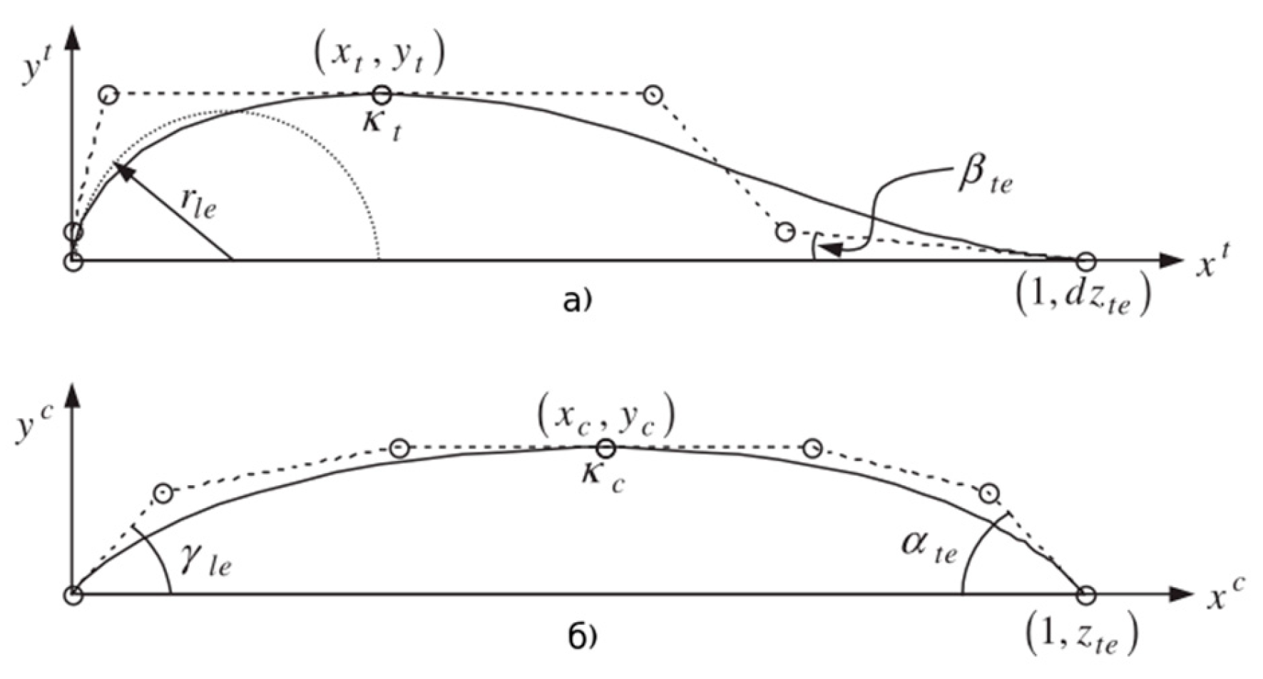
The third-degree Bezier curves are given by the following parametric equations (x(u) and y(u)):
where u is a parameter that changes from 0 to 1 under its own conditions.
The Bezier control points for the leading edge thickness line are calculated by the following equations:
and the control points of the trailing edge thickness line are calculated using:
the parameter b9 is the smallest root of:
and fulfill the condition of
The Bezier control points for the camber line at the leading edge are calculated using the following relations:
the parameter b1 is calculated from:
and must comply with 0 < b1 < yc.
And the curvature line control points at the trailing edge are calculated using:
Appendix C
| Algorithm C1. CAPR-SHADOW + GAN + AZTLI-NN algorithm [55]. | |
| Inputs: Ω, cy,d, αmax, yt,min M, Re, G, NP, NPmin, U*, γ, H, p | |
| Outputs: L(ξopt), ξopt | |
| 1 | Download the parameter normalization model; |
| 2 | Download AZTLI-NN architecture and Weights; |
| 3 | g = 1; |
| 4 | Initialize the Pg aggregate using GAN; |
| 5 | Normalize the parameters of the CST vectors of the initial population;; |
| 6 | Create images of graphs of aerodynamic coefficients using AZTLI-NN; |
| 7 | for i = 1 to NP do |
| 8 | Divide the images into three layers; |
| 9 | Get αi(cl,d) with the graph (cl vs α)i; |
| 10 | Get (αi(cl,d)) with the graph (cl1.5/cd vs α)i; |
| 11 | Apply (A7), to obtain max(yt(x))i; |
| 12 | Get ψ(ξg) with (32); |
| 13 | Get L(ξg) with (31); |
| 14 | Update U*; |
| 15 | mean(L(ξg))→ Lavg; |
| 16 | Assign values of 0,5 in memories MCR and MF; |
| 17 | Create A = ∅, |A| = round(2,6NP); |
| 18 | k = 1; |
| 19 | for g = 2 to G do |
| 20 | SCR = ∅, SF = ∅, Δf = ∅; |
| 21 | for i = 1 to NP do |
| 22 | ri = choose randomly from [1, H]; |
| 23 | Get CRi,g with (20); |
| 24 | Get Fi,g with (21); |
| 25 | Get the mutated vector vi,g with(22); |
| 26 | for j = 1 to |ξ| do |
| 27 | Get the component of the trial vector uj,i,g with (23); |
| 28 | Create images of graphs of aerodynamic coefficients of P(ug) using AZTLI-NN; |
| 29 | for i = 1 to NP do |
| 30 | Divide the images into three layers (from ug); |
| 31 | Get αi(cl,d) with the graph (cl vs α)i; |
| 32 | Get (αi(cl,d)) with the graph (cl1.5/cd vs α)i; |
| 33 | Apply (A7), to obtain max(yt(x))i; |
| 34 | Get ψ(ug) with (32); |
| 35 | Get L(ug) with (32); |
| 36 | Update U*; |
| 37 | for i = 1 to NP do |
| 38 | if L(ui,g) ≤ L(ξi,g) then |
| 39 | ξi,g+1 = ui,g; |
| 40 | ξi,g→ A; |
| 41 | CRi,g→ SCR, Fi,g→ SF; |
| 42 | |L(ui,g) - L(ξi,g)|→ Δf; |
| 43 | else |
| 44 | ξi,g+1 = ξi,g; |
| 45 | Update the memories MCR and MF with Algorithm 1; |
| 46 | mean(L(ξg+1))→ Lavg; |
| 47 | if g ≥ 3 then |
| 48 | Get Δg and Δg-1 with (30); |
| 49 | Get NPg+1 with (28); |
| 50 | if NPg+1 < NPmin then |
| 51 | Apply (29); |
| 52 | (NPg – NPg+1) worst elements → A; |
| 53 | if |A| > round(2,6NP) then |
| 54 | Delete (|A| - round(2,6NP)) elements randomly; |
| 55 | k++; |
| 56 | return Output |
Appendix D
| Algorithm D1. NSGA-II + GAN + AZTLI-NN algorithm [55]. | |
| Inputs: Ω, cy,d, M, Re, T, NP | |
| Outputs: FPareto(ξ), ξPareto | |
| 1 | Download the parameter normalization model; |
| 2 | Download AZTLI-NN architecture and weights; |
| 3 | t = 1; |
| 4 | Initialize the Pt aggregate using GAN; |
| 5 | Normalize the parameters of the CST vectors of the initial population;; |
| 6 | Create images of graphs of aerodynamic coefficients using AZTLI-NN; |
| 7 | for i = 1 to NP do |
| 8 | Divide the images into three layers; |
| 9 | Get αi(cl,d) with the graph (cl vs α)i; |
| 10 | Get (αi(cy,d)) with the graph (cl1.5/cd vs α)i; |
| 11 | Get |cm|(αi(cy,d)) with (cm vs α)p; |
| 12 | Get ranks Fi from Pt with Algorithm 2; |
| 13 | for i = 1 to maxrank do |
| 14 | Get CDi with Algorithm 3; |
| 15 | Sort Pt based on Fi and CDi; |
| 16 | while |Qt| < NP do |
| 17 | Get p1 with Algorithm 4; |
| 18 | Get p2 with Algorithm 4; |
| 19 | v1 = v2 = ∅; |
| 20 | for j = 1 to |p1| do |
| 21 | Get c1,j and c2,j with (35) and (36); |
| 22 | Get v1,j and v2,j with (37) and (38) |
| 23 | v1,j→v1; |
| 24 | v2,j→v2; |
| 25 | v1→Qt; |
| 26 | v2→Qt; |
| 27 | Rt = Pt ∪ Qt; |
| 28 | Get ranks Fi from Rt with Algorithm 2; |
| 29 | for i = 1 to maxrank do |
| 30 | Get CDi with Algorithm 3; |
| 31 | Sort Rt based on Fi and CDi; |
| 32 | Best NP vectors pass Rt→Pt+1; |
| 33 | Pt = Pt+1; |
| 34 | for t = 2 to T do |
| 35 | while |Qt| < NP do |
| 36 | Get p1 with Algorithm 6; |
| 37 | Get p2 with Algorithm 6; |
| 38 | v1 = v2 = ∅; |
| 39 | for j = 1 to |p1| do |
| 40 | Get c1,j and c2,j with (35) and (36); |
| 41 | Get v1,j and v2,j with (37) and (38); |
| 42 | v1,j→v1; |
| 43 | v2,j→v2; |
| 44 | v1→Qt; |
| 45 | v2→Qt; |
| 46 | Rt = Pt ∪ Qt; |
| 47 | Get ranks Fi from Rt with Algorithm 2; |
| 48 | for i = 1 to maxrank do |
| 49 | Get CDi with Algorithm 3; |
| 50 | Sort Rt based on Fi and CDi; |
| 51 | Best NP vectors pass Rt→Pt+1; |
| 52 | Pt = Pt+1; |
| 53 | return Output |
References
- Ma, Y.; Elham, A. Designing high aspect ratio wings: a review of concepts and approaches. Progress in Aerospace. 2024, 145, 100983. [Google Scholar] [CrossRef]
- Martins, J.R.; Kennedy, G.; Kenway, G.K. High aspect ratio wing design: optimal aero structural trade offs for the next generation of materials. In 52nd Aerospace Sciences Meeting. USA. 13-17 January 2014.
- Vassberg, J.C.; Jameson, A. Industrial applications of aerodynamic shape optimization. In VKI Lecture-II. Belgium. 11 September 2018.
- Nikolaev, N.V. Optimization of airfoils along high-aspect-ratio wing of long-endurance aircraft in trimmed flight. Journal of Aerospace Engineering. 2019, 32, 04019090. [Google Scholar] [CrossRef]
- Anderson, J.D.; Bowden, M.L. Introduction to flight, 9th ed.; McGraw-Hill Higher Education: USA, 2021; pp. 508–513.
- Steinbuch, M.; Marcus, B.; Shepshelovich, M. Development of UAV wings-subsonic designs. In 41st Aerospace Sciences Meeting and Exhibit. USA. 6-9 January 2003.
- Park, K.; Kim, B.S. Optimal design of an airfoil plataform shapes with high aspect ratio using genetic algorithms. International Journal of Aerospace and Mechanical Engineering. 2013, 7, 584–590. [Google Scholar]
- Wang, L.; Zhang, H.; Wang, C.; Tao, J.; Lan, X.; Sun, G.; Feng, J. A review of intelligent airfoil aerodynamic optimization methods based on data-driven advanced models. Mathematics. 2024, 12, 1417. [Google Scholar] [CrossRef]
- Dussage, T.P.; Sung, W.J.; Pinon Fischer, O.J.; Mavris, D.N. A reinforcement learning approach to airfoil shape optimization. Scientific Reports. 2023, 13, 9753. [Google Scholar] [CrossRef]
- Yan, X.; Zhu, J.; Kuang, M.; Wang, X. ; Aerodynamic shape optimization using a novel optimizer based on machine learning techniques. Aerospace Science and Technology. 2019, 86, 826–835. [Google Scholar] [CrossRef]
- Skinner, S.N.; Zare-Behtash, H. State-of-the-art in aerodynamic shape optimization methods. Applied Soft Computing. 2018, 62, 933–962. [Google Scholar] [CrossRef]
- Li, J.; Du, X.; Martins, J.R. Machine learning in aerodynamic shape optimization. Progress in Aerospace Sciences. 2022, 134, 100849. [Google Scholar] [CrossRef]
- Hu, L.; Zhang, J.; Xiang, Y.; Wnag, W. Neural networks-based aerodynamic data modeling: a comprehensive review. IEEE Access. 2020, 8, 90805–90823. [Google Scholar] [CrossRef]
- UIUC Airfoil coordinates database. Available online: https://m-selig.ae.illinois.edu/ads/coord_database.html (accessed on 20 February 2024).
- The incomplete guide to airfoil usage. Available online: https://m-selig.ae.illinois.edu/ads/aircraft.html#conventional (accessed on 19 February 2024).
- Derksen, R.W.; Rogalsky, T. Bezier-PARSEC: an optimized aerofoil parameterization for design. Advances in Engineering Software. 2010, 41, 923–930. [Google Scholar] [CrossRef]
- Goodfellow, I.; Pouget-Abadie, J.; Mirza, M.; Xu, B.; Warde-Farley, D.; Ozair, S.; Bengio, Y. Generative adversarial networks. Communications of the ACM. 2020, 63, 139–144. [Google Scholar] [CrossRef]
- Creswell, A.; White, T.; Dumoulin, V.; Arulkumuran, K.; Sengupta, B.; Bharath, A.A. Generative adversarial networks: an overview. IEEE Signal Processing. 2018, 35, 53–68. [Google Scholar] [CrossRef]
- OpenFOAM v11 User Guide. Available online: https://doc.cfd.direct/openfoam/user-guide-v11/index (accessed on 20 March 2024).
- Welcome to pygmsh’ documentation! Available online: https://pygmsh.readthedocs.io/en/latest (accessed on 10 March 2024).
- Eleni, D.C.; Athanasios, T.I.; Dionissios, M.P. Evaluation of the turbulence models for the simulation of the flow over a National Advisory Committe for Aeronautics (NACA) 0012 airfoil. Journal of Mechanical Engineering Research. 2012, 4, 100–111. [Google Scholar]
- Suvanjumrat, C. Comparison of turbulence models for flow past NACA0015 airfoil using OpenFOAM. Engineering Journal. 2017, 21, 207–221. [Google Scholar] [CrossRef]
- Khan, S.A.; Bashir, M.; Baig, M.A.A.; Ali, F.A.G.M. Comparing the effect of different turbulence models on the CFD predictions of NACA0018 airfoil aerodynamics. CFD Letters. 2020, 3, 1–10. [Google Scholar] [CrossRef]
- Menter, F.R.; Kuntz, M.; Lagtry, R. ; Ten years of industrial experience with the SST turbulence model. Turbulence, heat and mass transfer. 2003, 4, 625–632. [Google Scholar]
- Lu, S.; Liu, J.; Hekkenberg, R. Mesh properties for RANS simulations of airfoil-shaped profiles: a case study of ruder hydrodynamics. Journal Marine Science and Engineering. 2021, 9, 1062. [Google Scholar] [CrossRef]
- Liu, F. A thorough description of how wall functions are implemented in OpenFOAM. In CFD with OpenSource Sotfware. 22 January 2017.
- Sola, J.; Sevilla, J. Importance of input data normalization for the application of neural networks to complex industrial problems. IEEE Transactions on Nuclear Science. 1997, 44, 1464–1468. [Google Scholar] [CrossRef]
- Gokhan, A.K.S.U.; Guzeller, C.O.; Eser, M.T. The effect of the normalization method used in different sample sizes on the success of artificial neural network model. International Journal of Assessment Tools in Education. 2019, 6, 170–192. [Google Scholar]
- Pedregosa, F.; Varoquax, G.; Gramfort, A.; Michel, V.; Thirion, B.; Grisel, O.; Blondel, M.; Prettenhofer, P.; Weiss, R.; Dubourg, V.; Vanderplas, J.; Passos, A.; Cournapeau, D.; Brucher, M.; Perrot, M.; Duchesnay, E. Scikit-learn: machine learning in Python. Journal of Machine Learning Research. 2011, 12, 2825–2830. [Google Scholar]
- Keras. Available online: https://keras.io (accessed on 15 April 2024).
- Wang, J.; He, C.; Li, R.; Chen, H.; Zhai, C.; Zhang, M. Flow field predictions of supercritical airfoils via variational autoencoder based deep learning framework. Physics Fluids. 2021, 33, 086108. [Google Scholar] [CrossRef]
- Tharwat, A. Principal component analysis – a tutorial. International Journal of Applied Pattern Recognition. 2016, 3, 197–240. [Google Scholar] [CrossRef]
- Kingma, D.P.; Welling, M. An introduction to variational autoencoders. Foundations and Trends in Machine Learning. 2019, 12, 307–392. [Google Scholar] [CrossRef]
- Espinosa Barcenas, O.U.; Quijada Pioquinto, J.G.; Kurkina, E.; Lukyanov, O. Surrogate aerodynamic wing modeling based on a multilayer perceptron. Aerospace. 2023, 10, 149. [Google Scholar] [CrossRef]
- Sun, G.; Sun, Y.; Wang, S. Artificial neural network based inverse design: airfoils and wings. Aerospace Science and Technology. 2015, 42, 415–428. [Google Scholar] [CrossRef]
- Moin, H.; Khan, H.Z.I.; Mobeen, S.; Riaz, J. Airfoil’s aerodynamic coefficients prediction using artificial neural network. In 2022 19th International Bhurban Conference on Applied Sciences and Technology (IBCAST). Pakistan. 16 - 20 August 2022.
- Deng, C.; Zhao, B.; Yang, Y.; Deng, A. Integer encoding differential evolution algorithm for integer programming. In 2010 2nd International Conference on Information Engineering and Computer Science. China. 30 December 2010.
- Tanabe, R.; Fukunuga, A. Success-history based parameter adaptation for differential evolution. In IEEE Congress on Evolution Computation (CEC). Mexico. 15 July 2013.
- Tanabe, R.; Fukunuga, A.S. Improving the search performance of SHADE using linear population size reduction. In 2014 IEEE Congress on Evolution Computation (CEC). China. 22 September 2014.
- Renkavieski, C.; Parpinelli, R.S. L-SHADE with alternative population size reduction for unconstrained continuous optimization. Anais do Computer on the Beach. 2020, 11, 351–358. [Google Scholar]
- Wong, I.; Liu, W.; Ho, C.M.; Ding, X. Continuous adaptive population reduction (CAPR) for differential evolution optimization. SLAS Technology. 2017, 22, 289–305. [Google Scholar] [CrossRef] [PubMed]
- Pioquinto, J.G.Q.; Moreno, R.A.F. Methods for increasing the efficiency of the differential evolution algorithm for aerodynamic shape optimization applications. In the XXVI All-Russian Seminar on Motion Control and Navigation of Aircraft. Russia. 14-16 June 2023.
- Sedelnikov, A.; Kurkin, E.; Quijada Pioquinto, J.G.; Lukyanov, O.; Nazarov, D.; Chertykovtseva, V.; Kurkina, E.; Hoang, V.H. Algorithm for propeller optimization based on differential evolution. Computation. 2024, 12, 52. [Google Scholar] [CrossRef]
- Ali, M.M.; Zhu, W.X. A penalty function-based differential evolution algorithm for constrained global optimization. Comput. Optim. Appl. 2013, 54, 707–739. [Google Scholar] [CrossRef]
- Deb, K.; Pratab, A.; Agarwal, S.; Meyarivan, T.A.M.T. A fast and elitist multiobjective genetic algorithm: NSGA-II. IEEE Transactions on Evolutionary Computation. 2002, 6, 182–197. [Google Scholar] [CrossRef]
- Verma, S.; Pant, M.; Snasel, V. A comprehensive review on NSGA-II for multi-objective combinatorial optimization problems. IEEE Access. 2021, 9, 57757–57791. [Google Scholar] [CrossRef]
- Deb, K.; Sindhya, K.; Okabe, T. Self-adaptive simulated binary crossover for real-parameter optimization. In the 9th Annual Conference on Genetic and Evolutionary Computation. 7 July 2007.
- Kakde, M.R.O. Survey on multiobjective evolutionary and real coded genetic algorithms. In the 8th Asia Pacific Symposium on Intelligent and Evolutionary Systems. January 2004.
- Das, S.; Mullick, S.S.; Suganthan, P.N. Recent advances in differential evolution – an update survey. Swarm and Evolutionary Computation. 2016, 27, 1–30. [Google Scholar] [CrossRef]
- Ladson, C.L. Effects of independent variation of Mach and Reynolds numbers on the low-speed aerodynamic characteristics of the NACA 0012 airfoil section. National Aeronautics and Space Administration, Scientific and Technical Information Division. 1988. № 4074.
- Turbulent flow over NACA0012 airfoil (2D). Available online: https://www.openfoam.com/documentation/guides/latest/doc/verification-validation-naca0012-airfoil-2d.html (accessed on 20 March 2024).
- Althaus, D.; Wortmann, F.X. Experimental results from laminar wind tunnel of the Institut fur Aero- und Gasdynamic der Universitat Stuttgart. Fried. Vieweg & Sohn: Germany, 1981; 1-20.
- Kulfan, B.M.; Bussoletti, J.E. “Fundamental” parametric geometry representations for aircraft component shapes. In 11th AIAA/ISSMO Multidisciplinary Analysis and Optimization Conference. USA. 6-8 September 2006.
- Rogalsky, T. Acceleration of differential evolution for aerodynamic design. PhD Thesis, . Winnipeg, Canada, March 2004. [Google Scholar]
- OpenVozduj/AZTLI-NN. Available online: https://github.com/OpenVozduj/AZTLI-NN (accessed on 22 July 2024).
Figure 1.
General architecture of the architecture of a GAN.
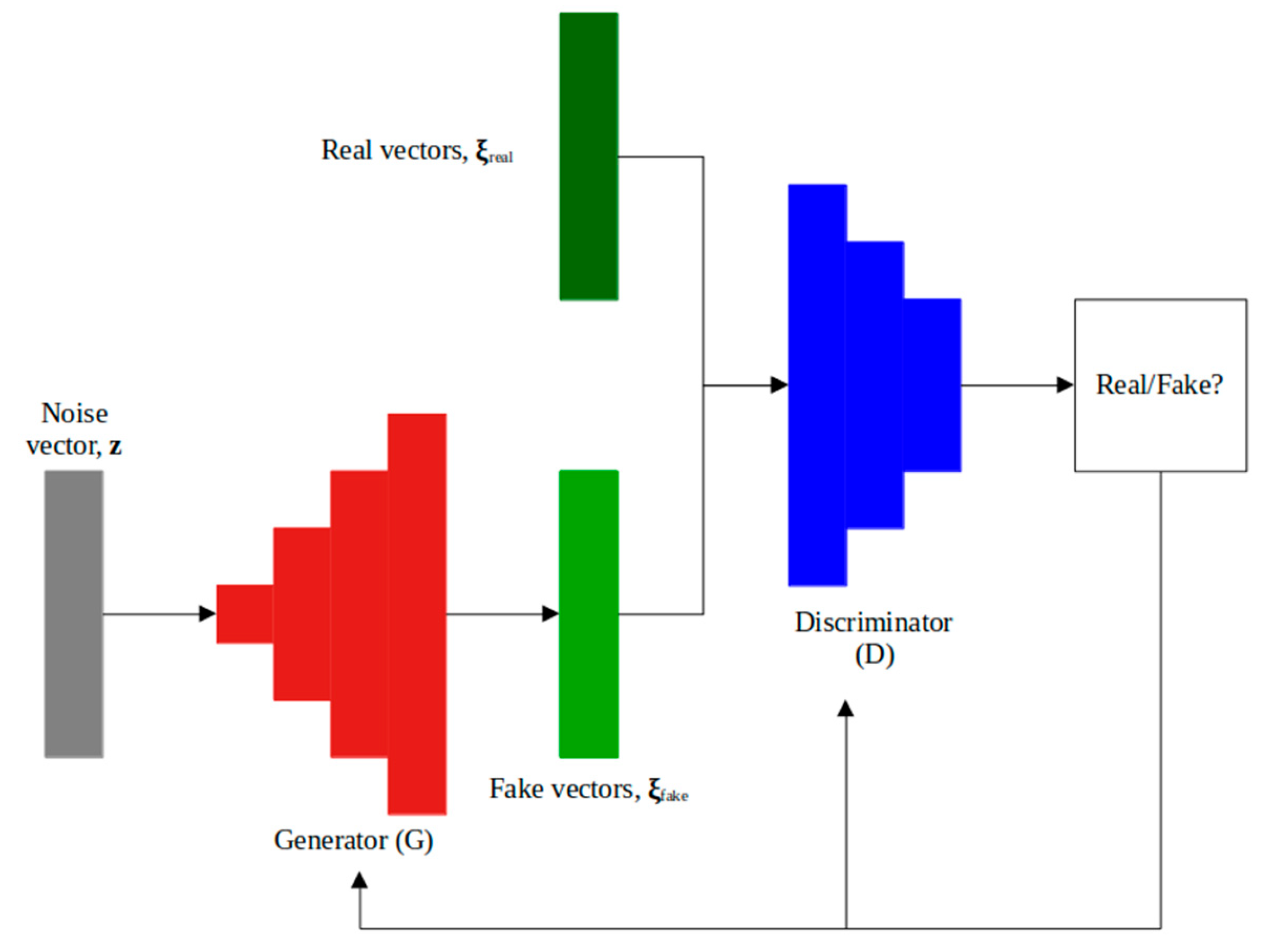
Figure 2.
(a) Dimensions of the control volume, c is the chord length of the profile; (b) General view of the mesh; (c) Boundary conditions of the control volume.
Figure 2.
(a) Dimensions of the control volume, c is the chord length of the profile; (b) General view of the mesh; (c) Boundary conditions of the control volume.
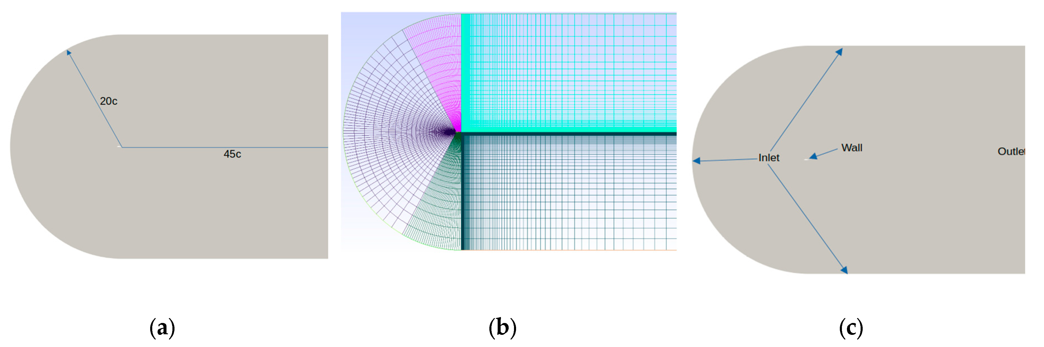
Figure 3.
Creation of the output data (output images) representing the aerodynamic coefficients of the airfoils.
Figure 3.
Creation of the output data (output images) representing the aerodynamic coefficients of the airfoils.
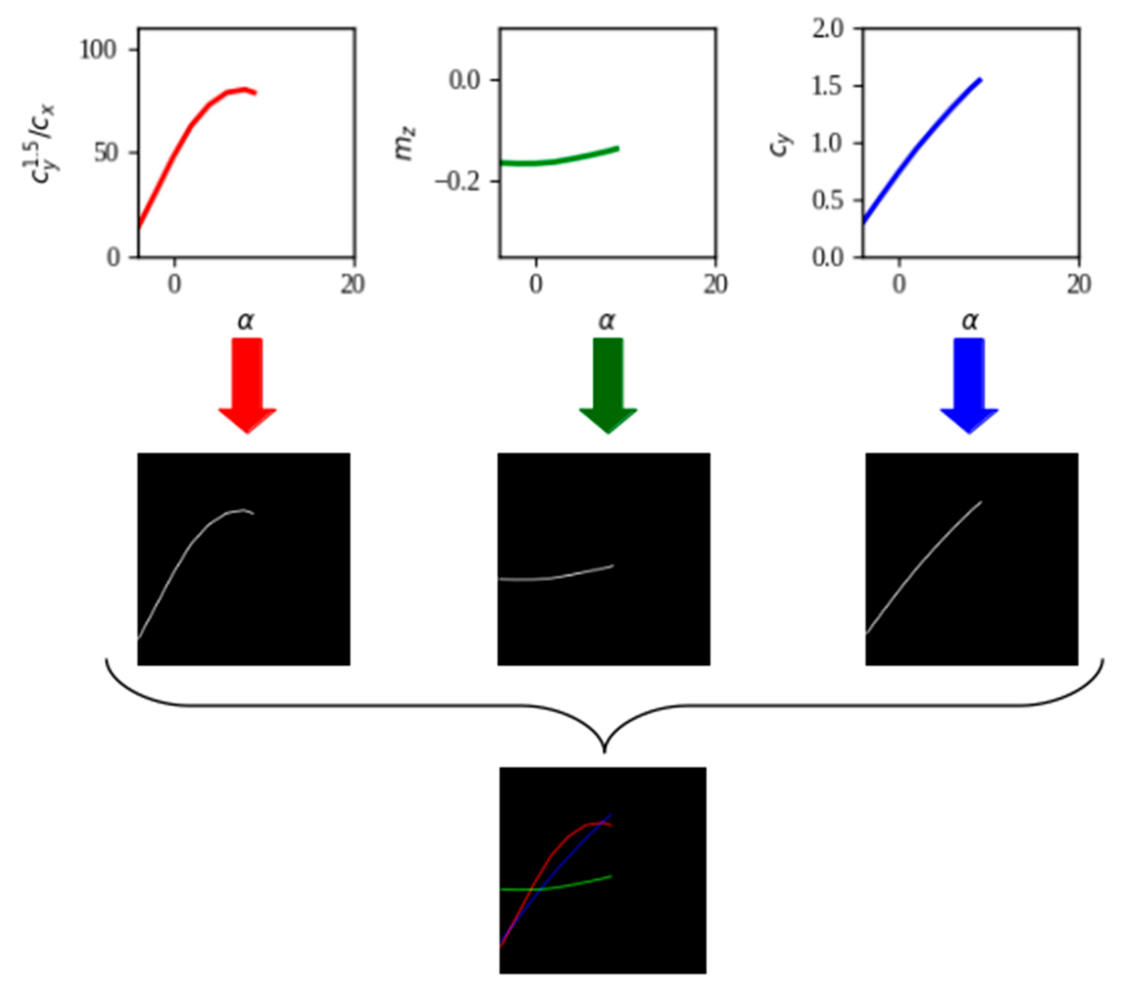
Figure 4.
Methodology of design of a neural network to predict aerodynamic coefficients.
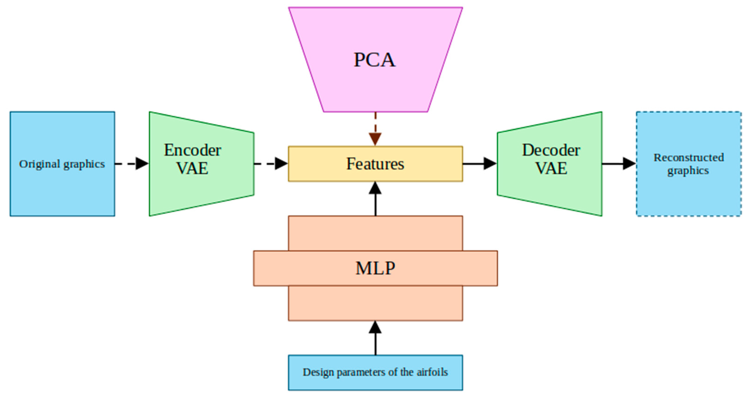
Figure 5.
General architecture of a VAE.
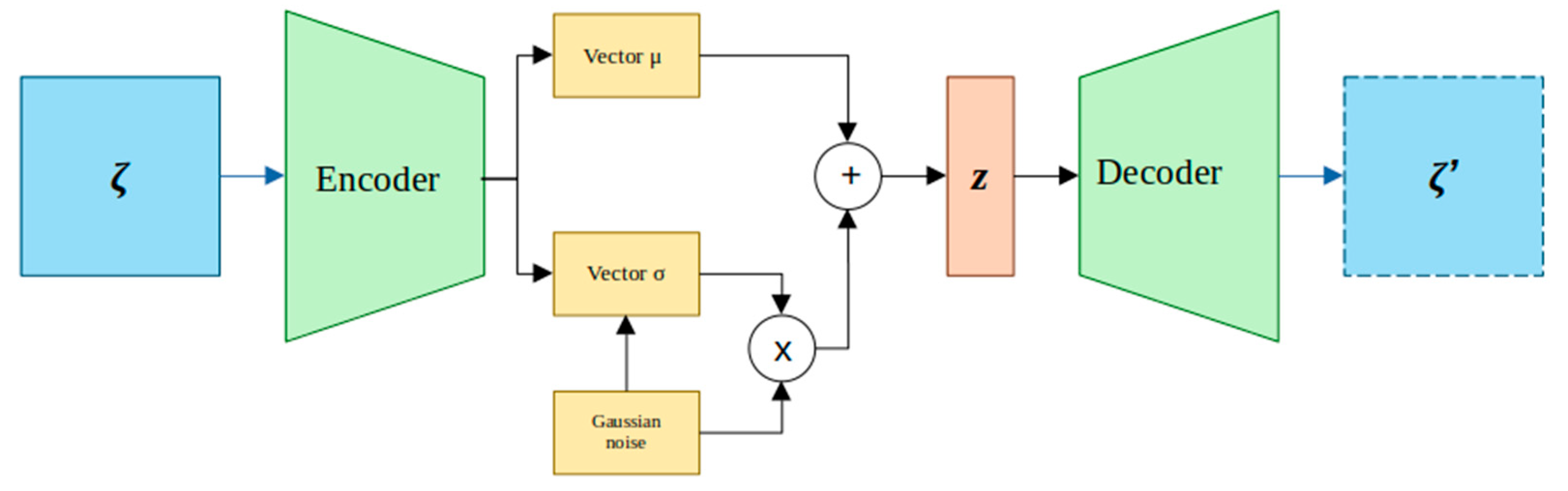
Figure 6.
Architecture of the encoder.
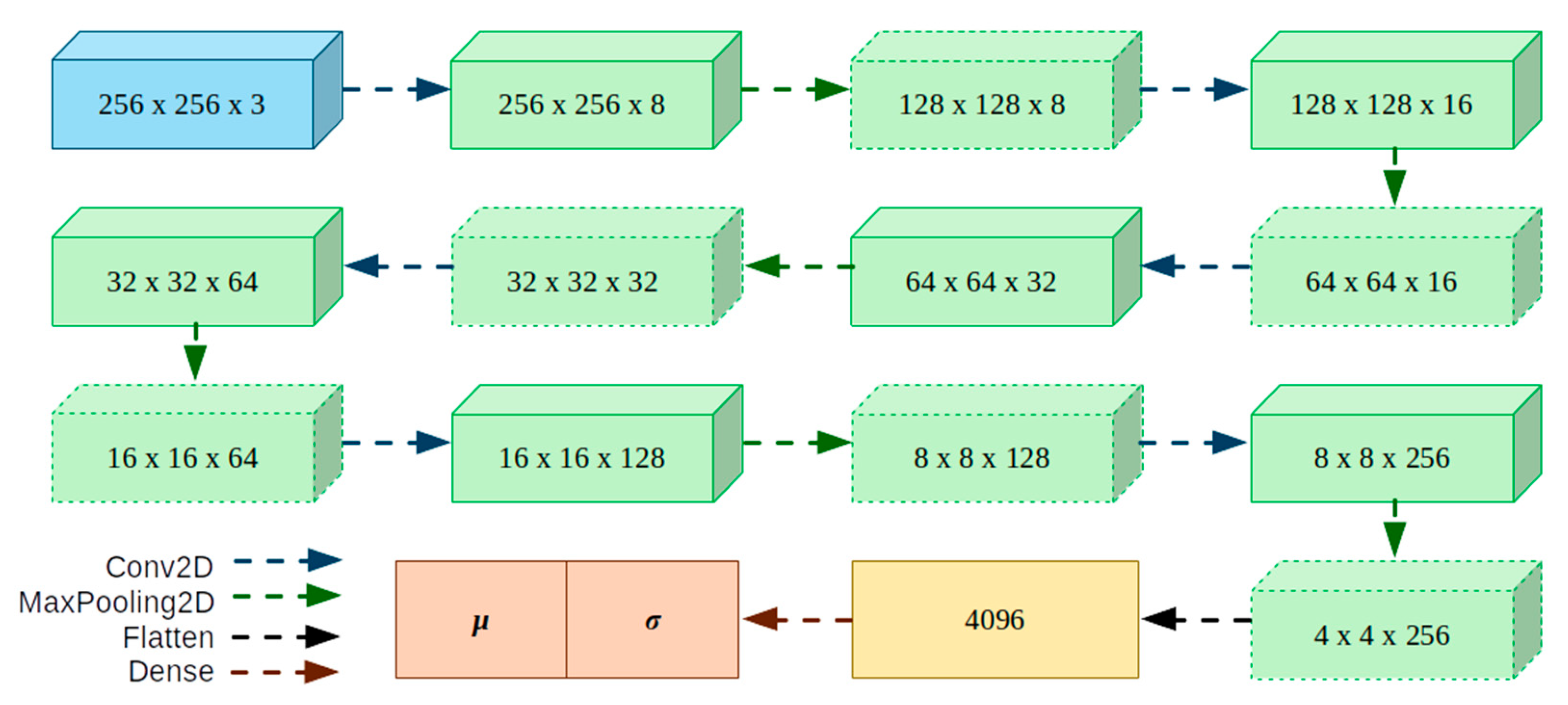
Figure 7.
Architecture of the decoder.
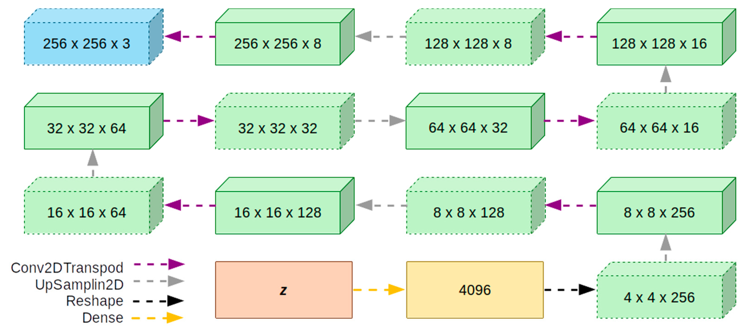
Figure 8.
Final architecture of the neural network “AZTLI-NN” used to predict aerodynamic coefficients of the airfoils.
Figure 8.
Final architecture of the neural network “AZTLI-NN” used to predict aerodynamic coefficients of the airfoils.
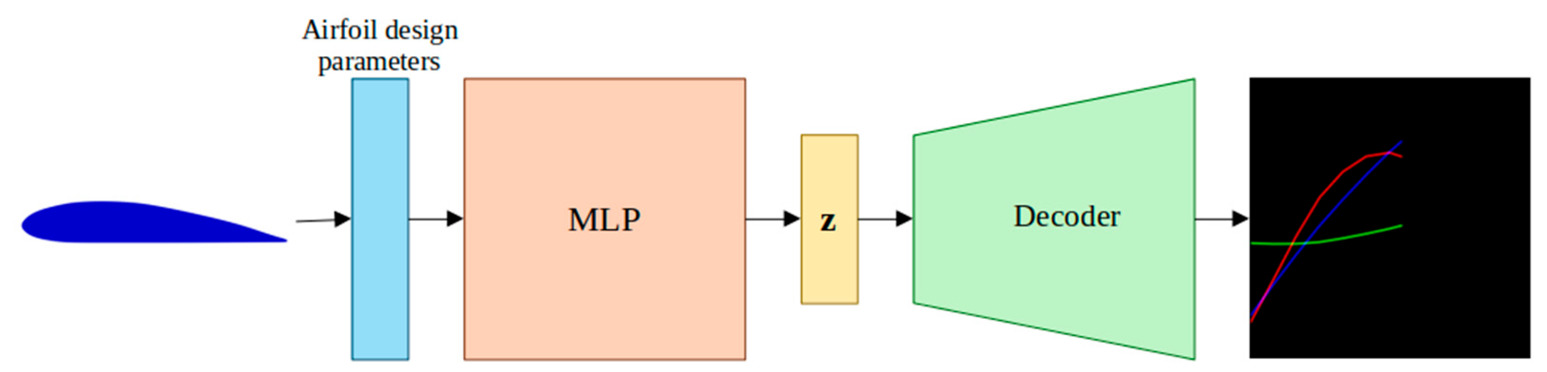
Figure 9.
(a) non-dominated classification; (b) crowding distance.
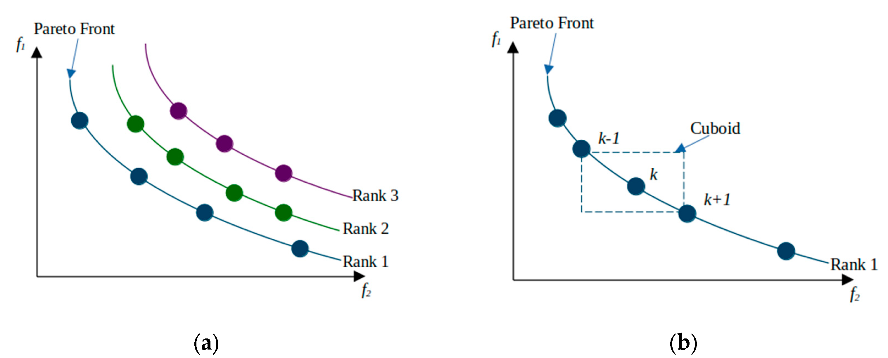
Figure 10.
The procedure for conducting NSGA-II.
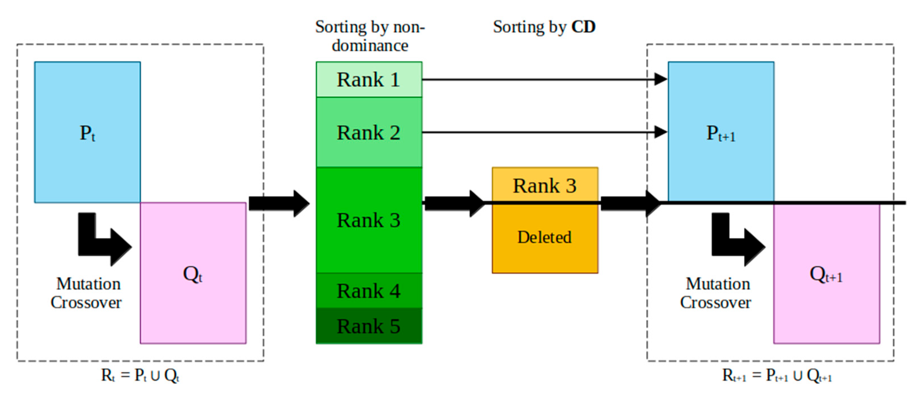
Figure 11.
Results obtained from the airfoil reconstruction tests.
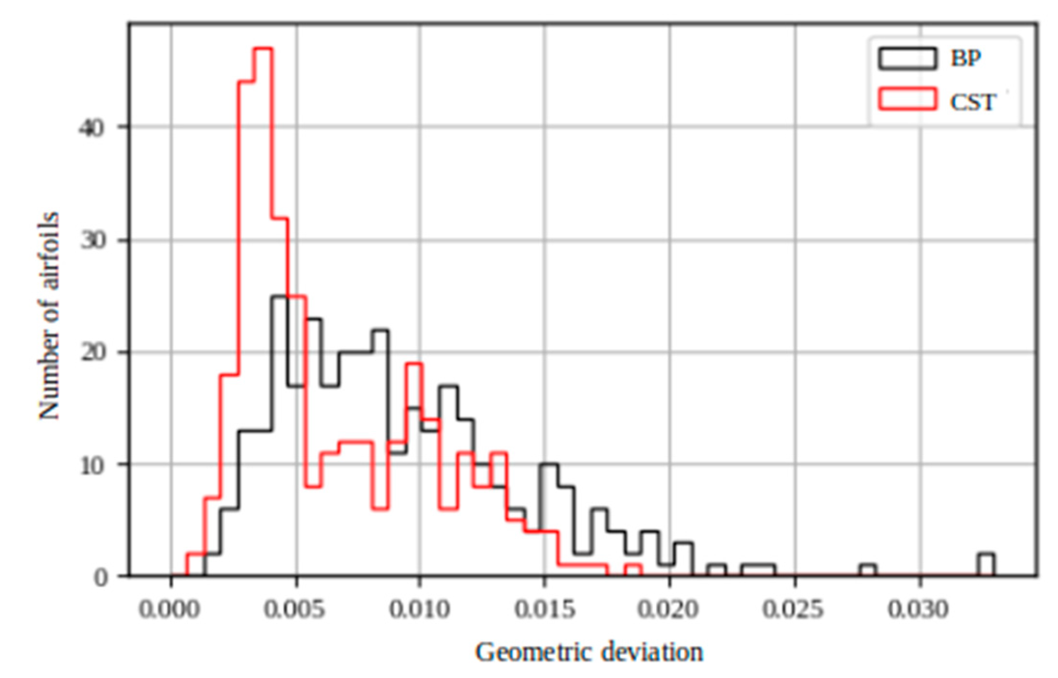
Figure 12.
Airfoils reconstructed using the Bezier-PARSEC method (black) and the CST method (red). The original coordinates are shown in green. (a) Eppler 407 airfoil, (b) Gottingen 621 airfoil, (c) NACA airfoil of the 5-digit series NACA23016, and (d) TSAGI 12 airfoil.
Figure 12.
Airfoils reconstructed using the Bezier-PARSEC method (black) and the CST method (red). The original coordinates are shown in green. (a) Eppler 407 airfoil, (b) Gottingen 621 airfoil, (c) NACA airfoil of the 5-digit series NACA23016, and (d) TSAGI 12 airfoil.
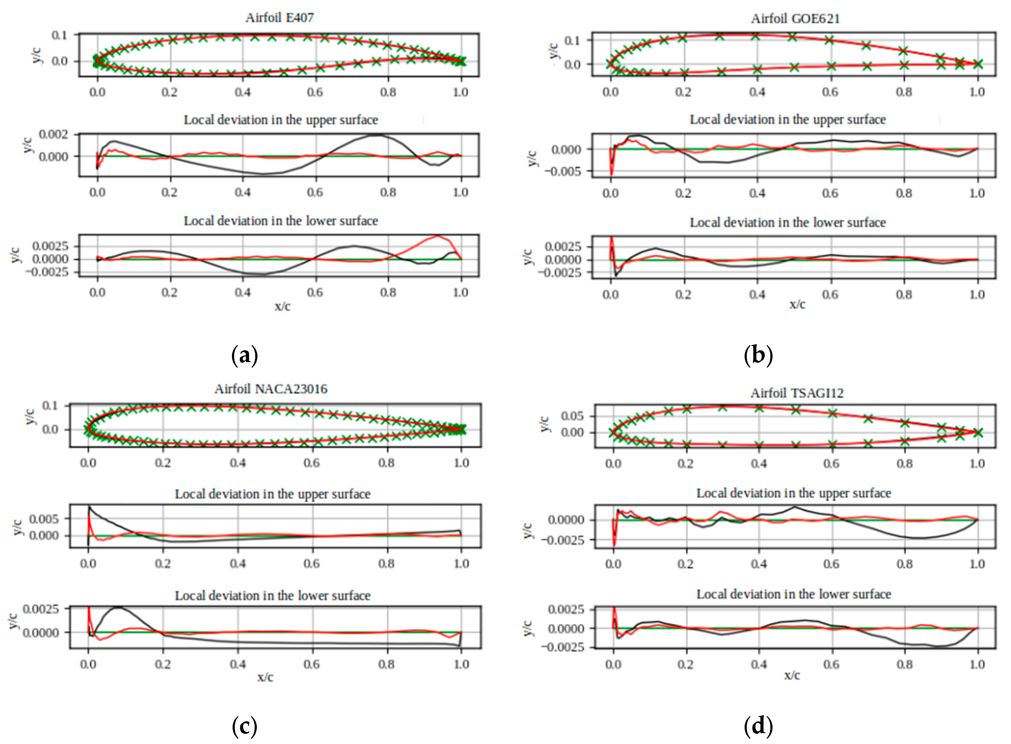
Figure 13.
Architecture of the GAN used to create new airfoils.
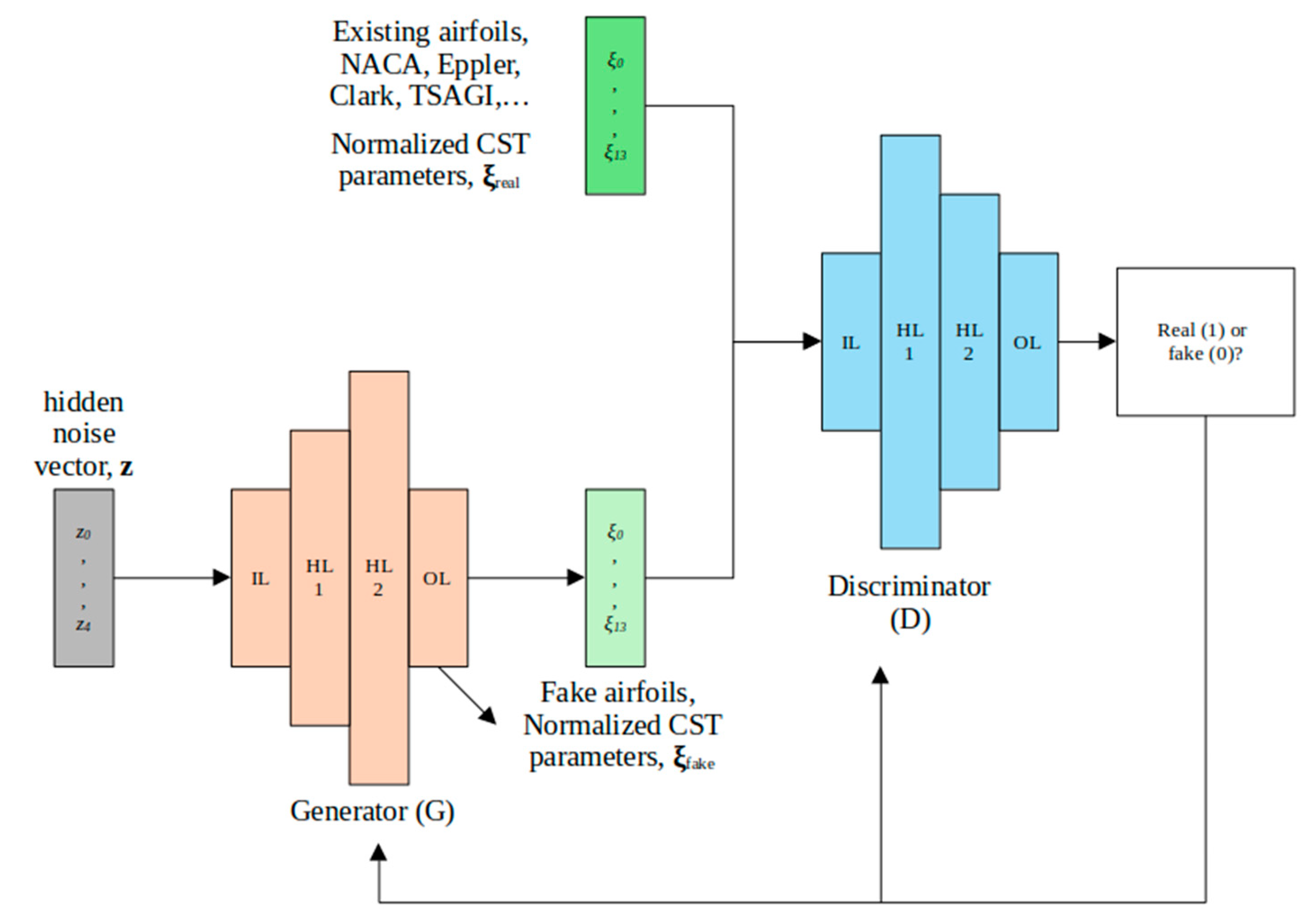
Figure 14.
Training of the GAN.
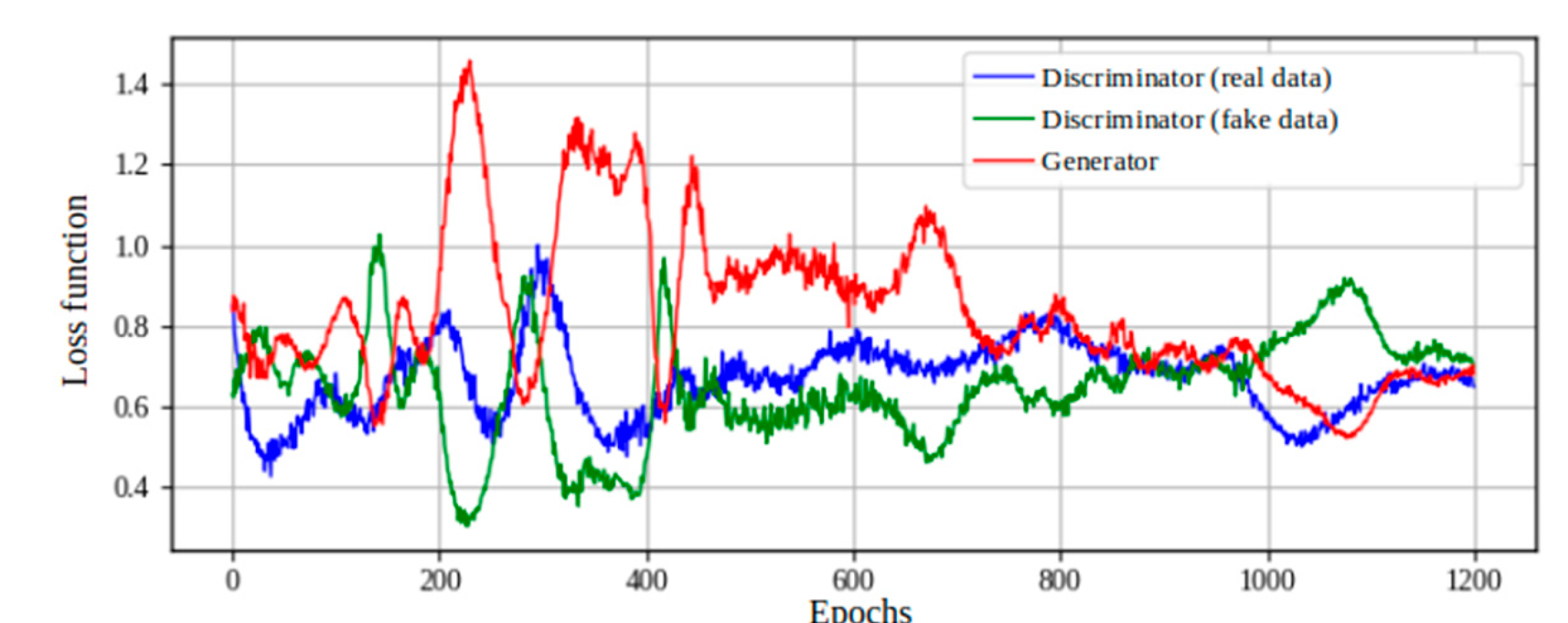
Figure 15.
Airfoils obtained after 1200 learning epochs.
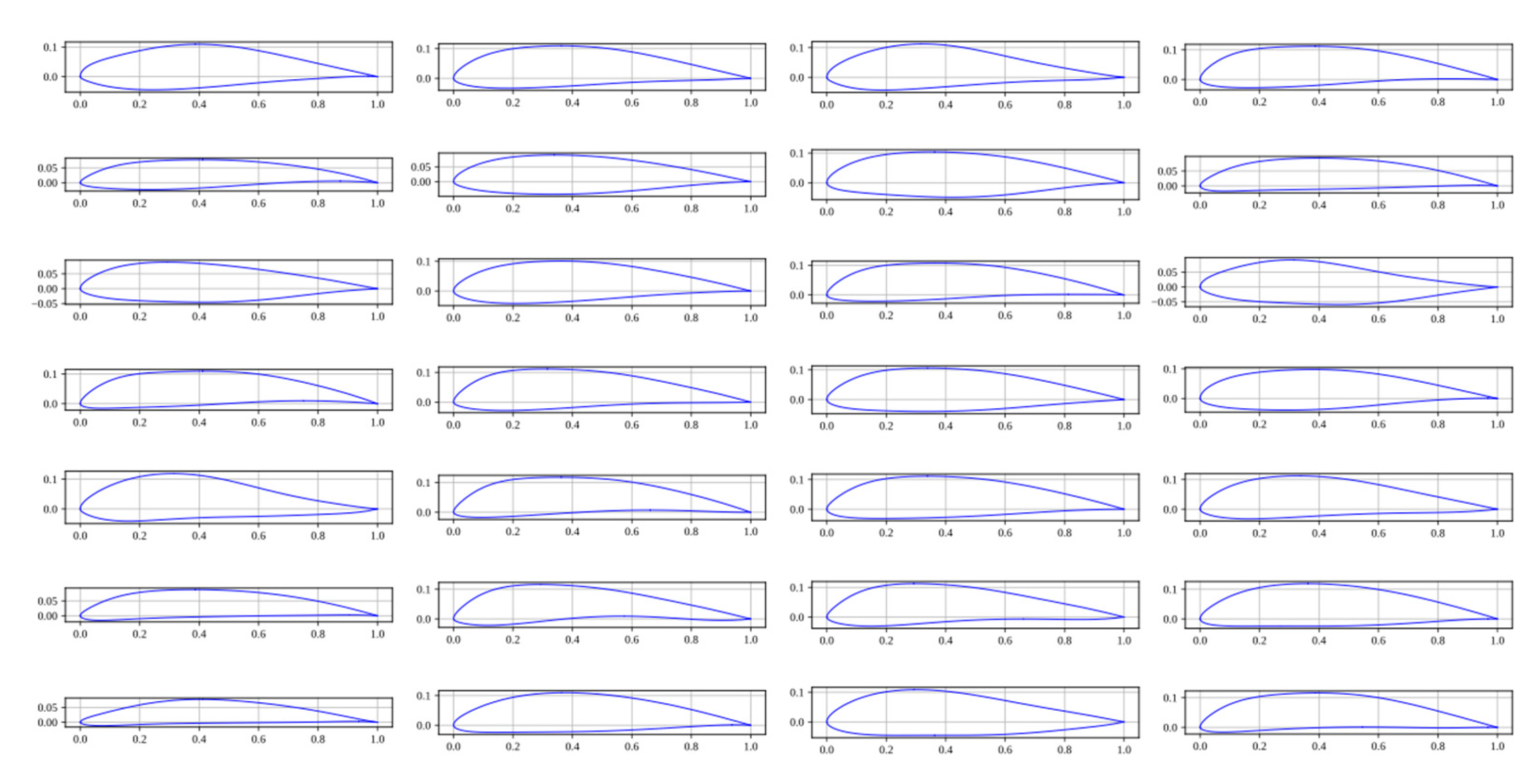
Figure 16.
Aerodynamic coefficients of the NACA 0012 airfoil.
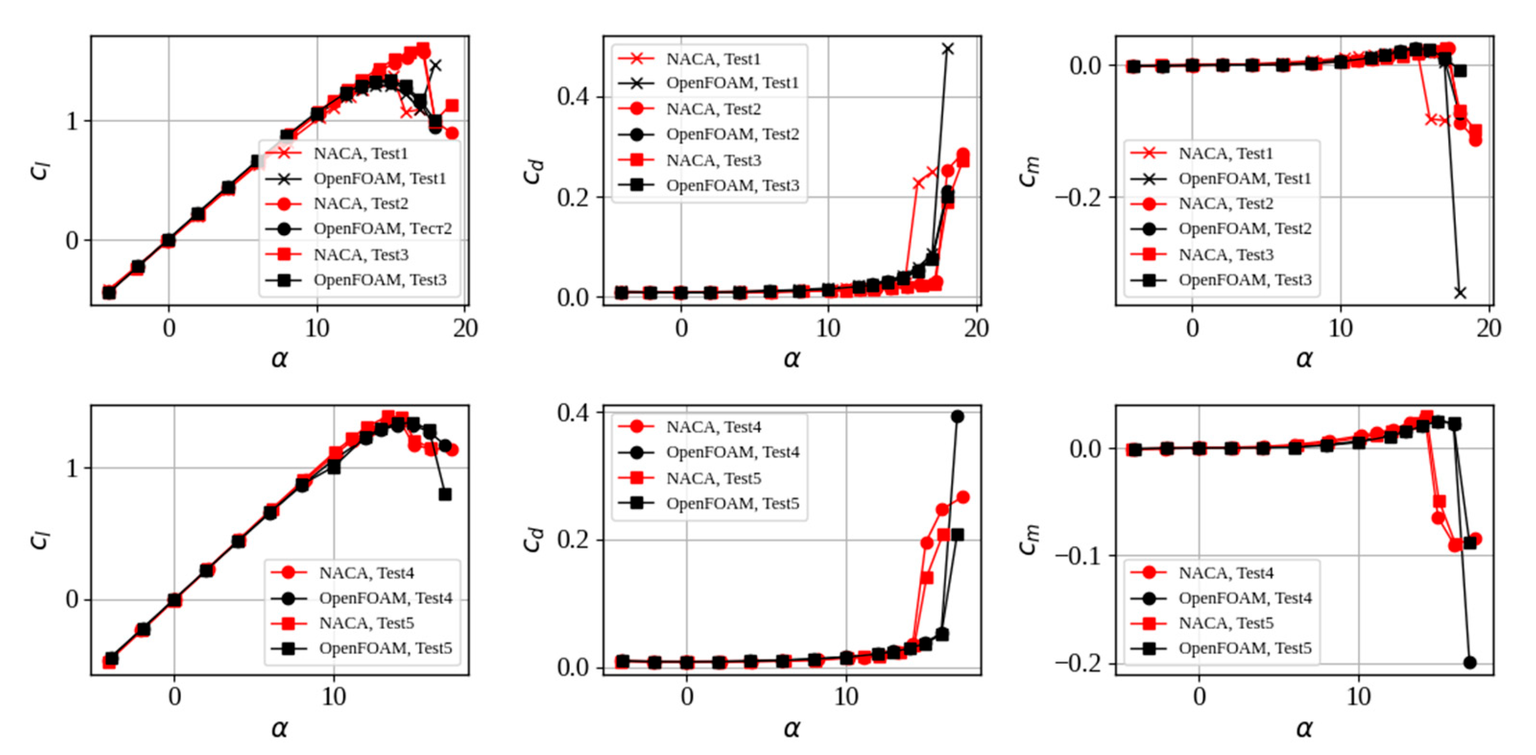
Figure 17.
Reconstruction of the graph of cl1.5/cd vs α by PCA using different number of PCs.
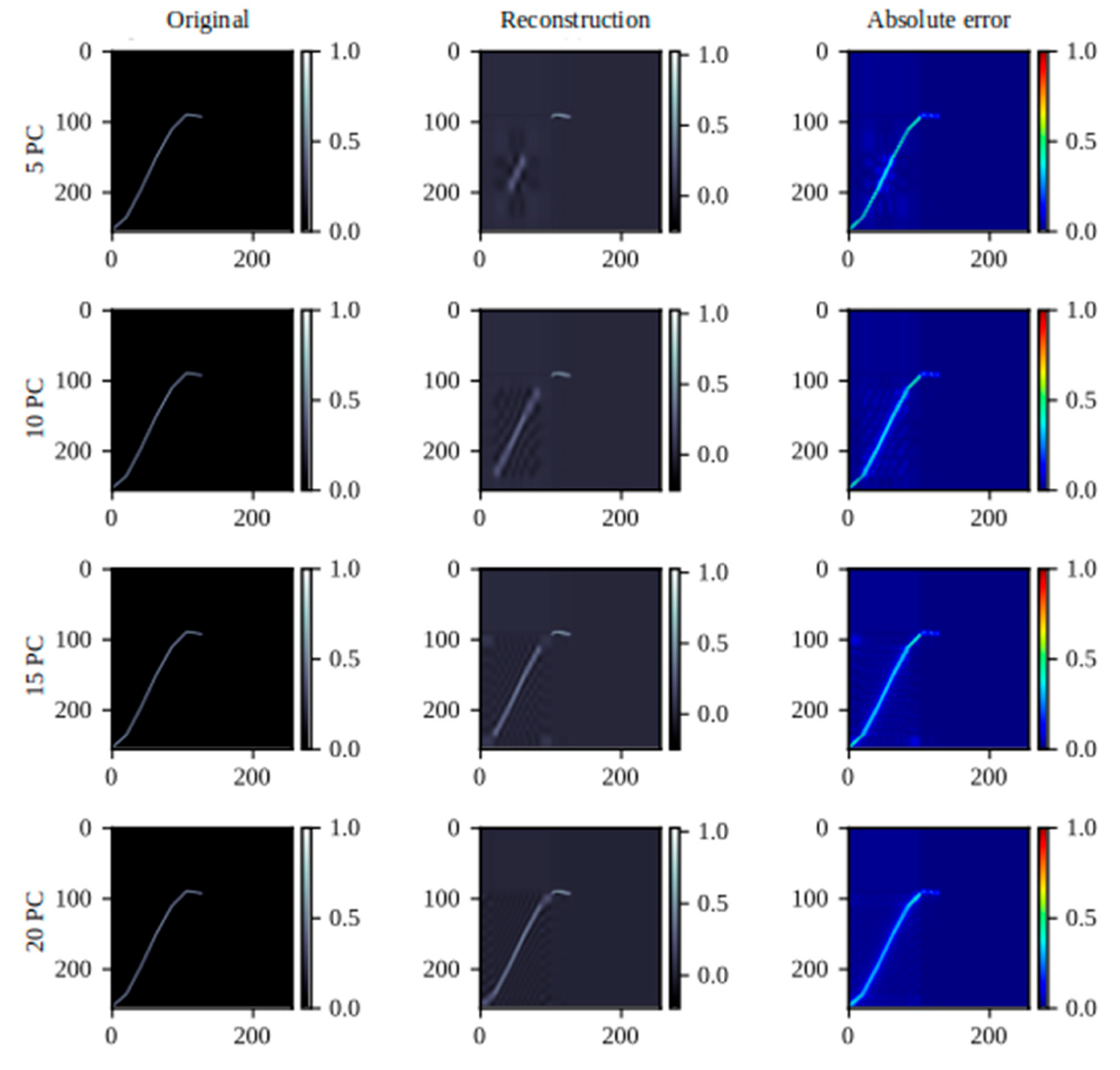
Figure 18.
Reconstruction of the graph of cm vs α by PCA using different number of PCs.
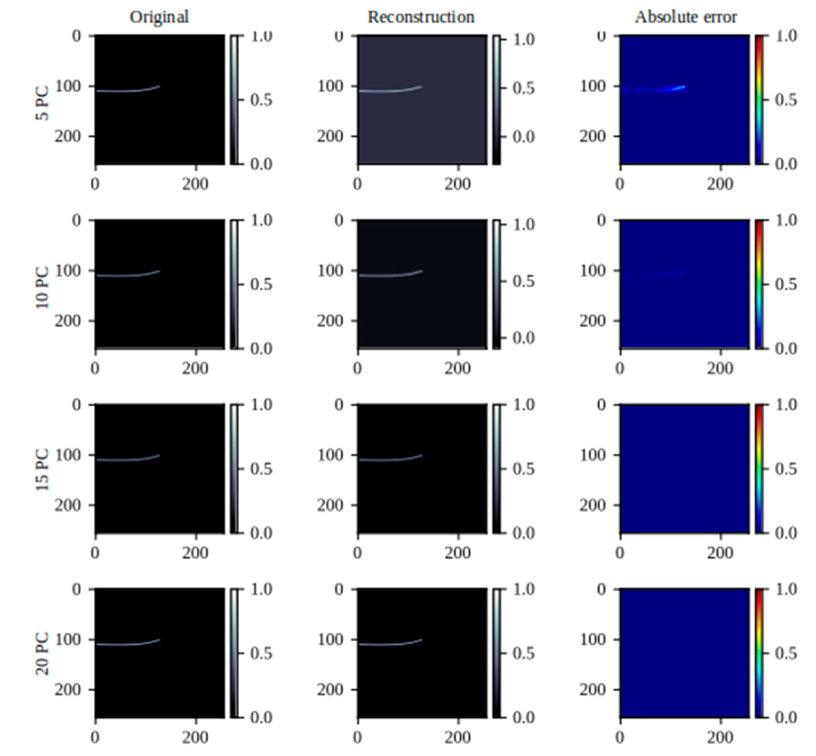
Figure 19.
Reconstruction of the graph of cl vs α by PCA using different number of PCs.
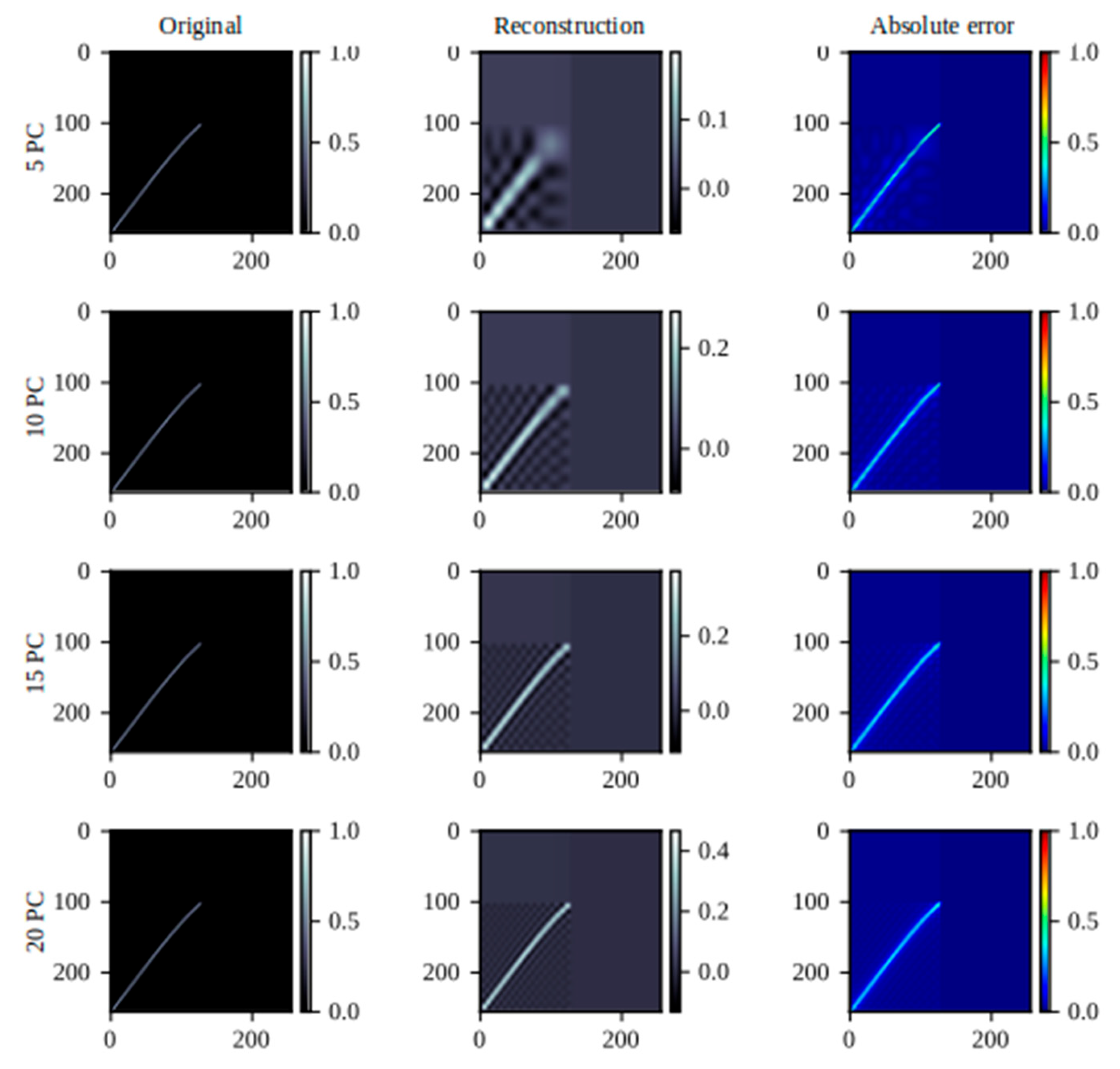
Figure 20.
Statistical distribution of MAE in the reconstruction of graphs with a VAE. Stage of training.
Figure 20.
Statistical distribution of MAE in the reconstruction of graphs with a VAE. Stage of training.
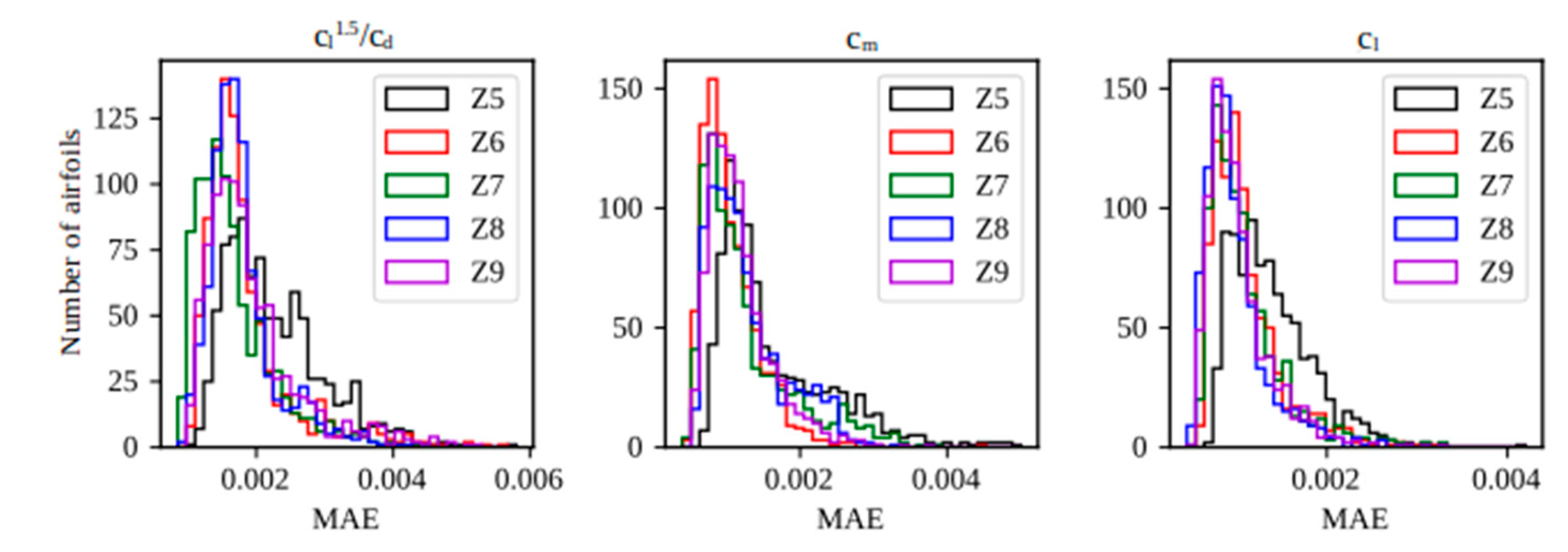
Figure 21.
Statistical distribution of MAE in the reconstruction of graphs with a VAE. Stage of testing.
Figure 21.
Statistical distribution of MAE in the reconstruction of graphs with a VAE. Stage of testing.
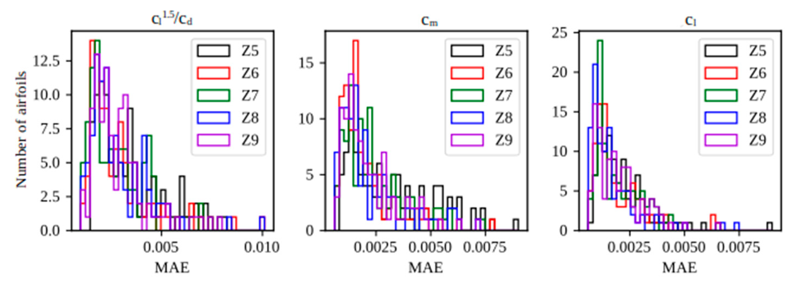
Figure 22.
Reconstruction of the graphs of the aerodynamic coefficients of the Eppler 502 airfoil (Re = 1.5x10⁶, M = 0.15).
Figure 22.
Reconstruction of the graphs of the aerodynamic coefficients of the Eppler 502 airfoil (Re = 1.5x10⁶, M = 0.15).
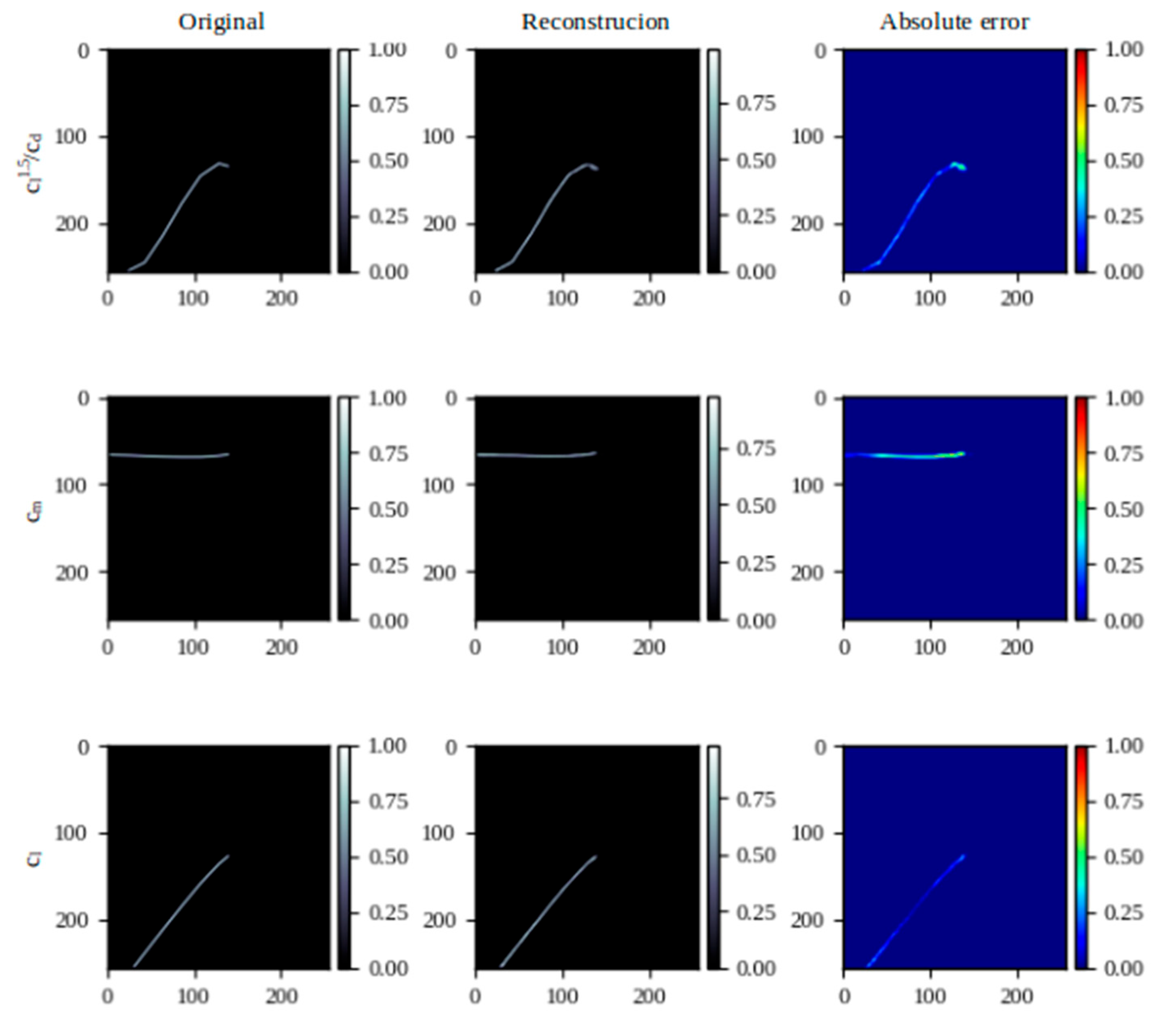
Figure 23.
Analysis of the performance in the reading of aerodynamic coefficients in the graphs reconstructed by the VAE.
Figure 23.
Analysis of the performance in the reading of aerodynamic coefficients in the graphs reconstructed by the VAE.
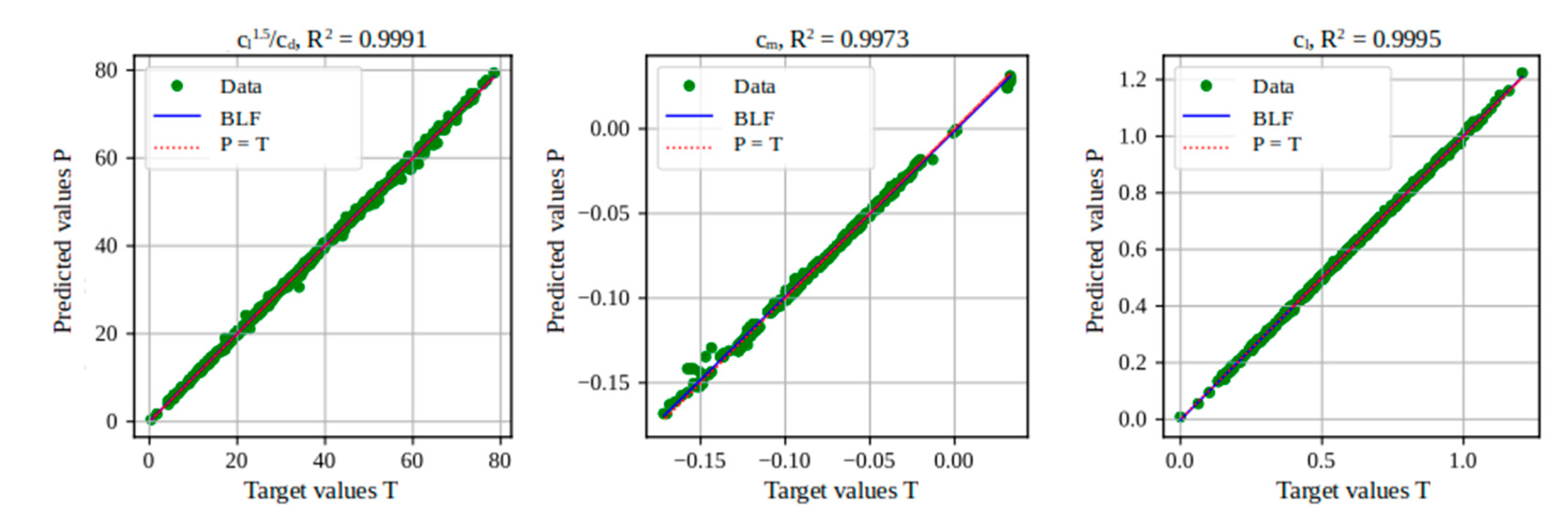
Figure 24.
The Architecture of MLP.
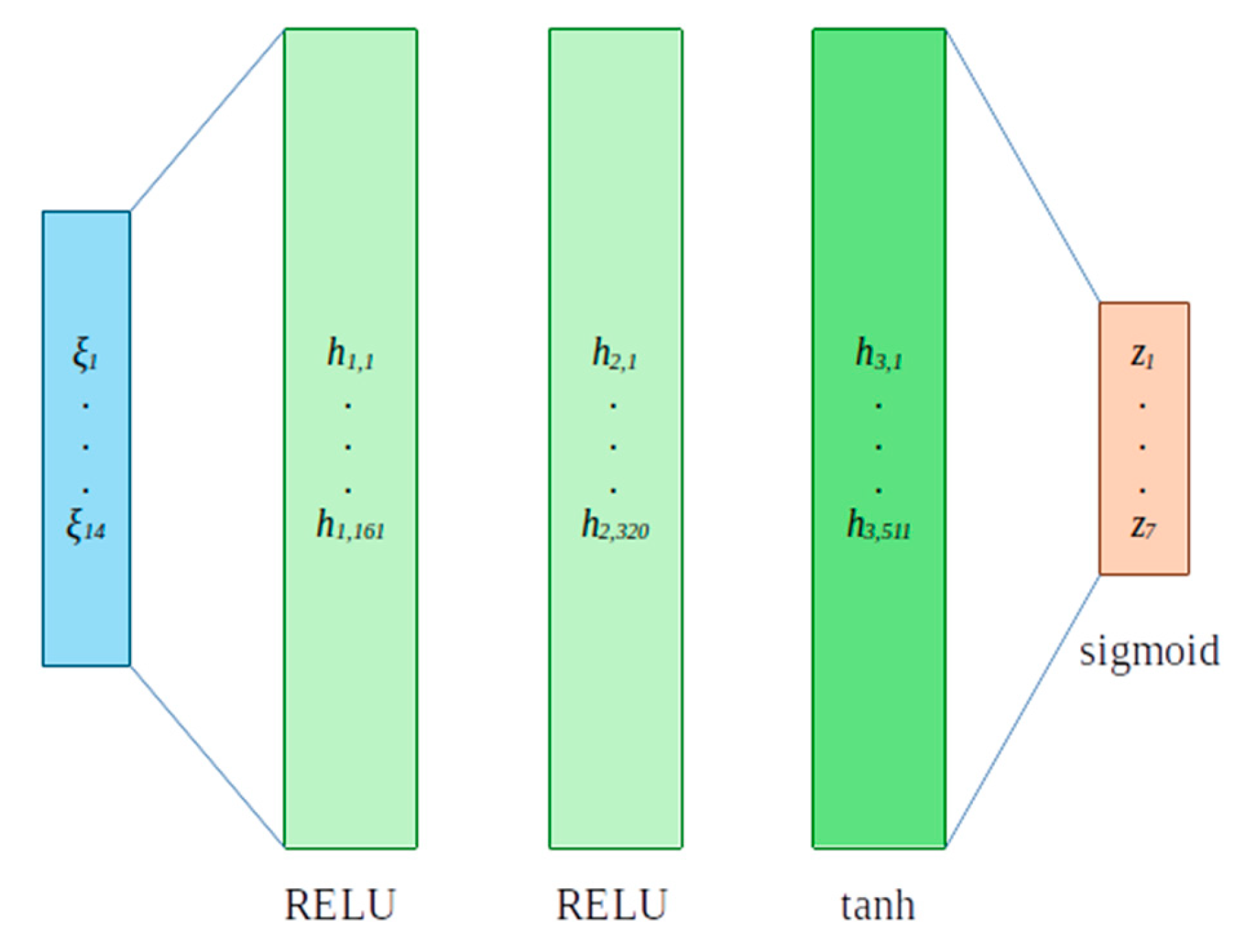
Figure 25.
Performance analysis in predicting aerodynamic coefficients using AZTLI-NN (1000 data).
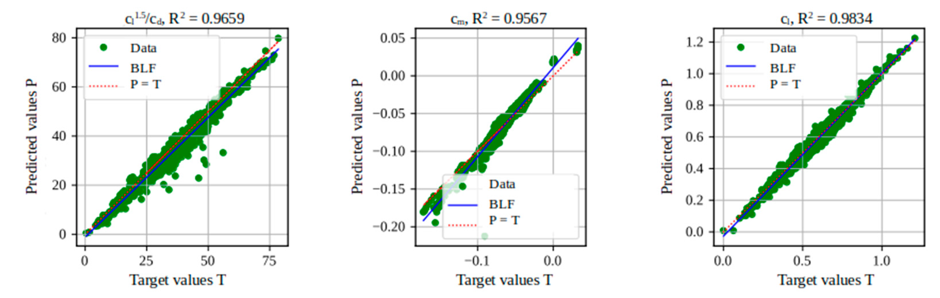
Figure 26.
Performance analysis in predicting aerodynamic coefficients using AZTLI-NN (1500 data).
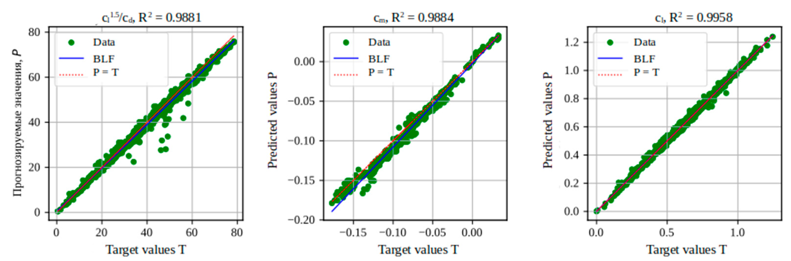
Figure 27.
Aerodynamic coefficients of the FX 66-S-161 profile obtained with a laminar wind tunnel, with OpenFOAM and with AZTLI-NN.
Figure 27.
Aerodynamic coefficients of the FX 66-S-161 profile obtained with a laminar wind tunnel, with OpenFOAM and with AZTLI-NN.
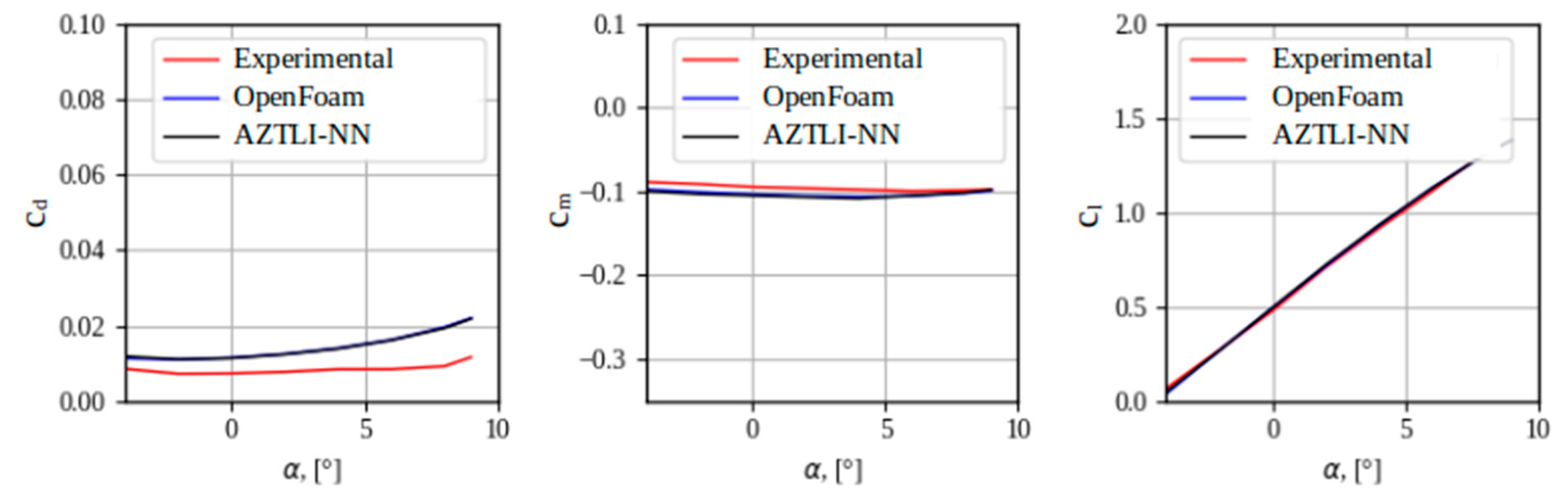
Figure 28.
Convergence analysis of the CAPR-SHADE algorithm.
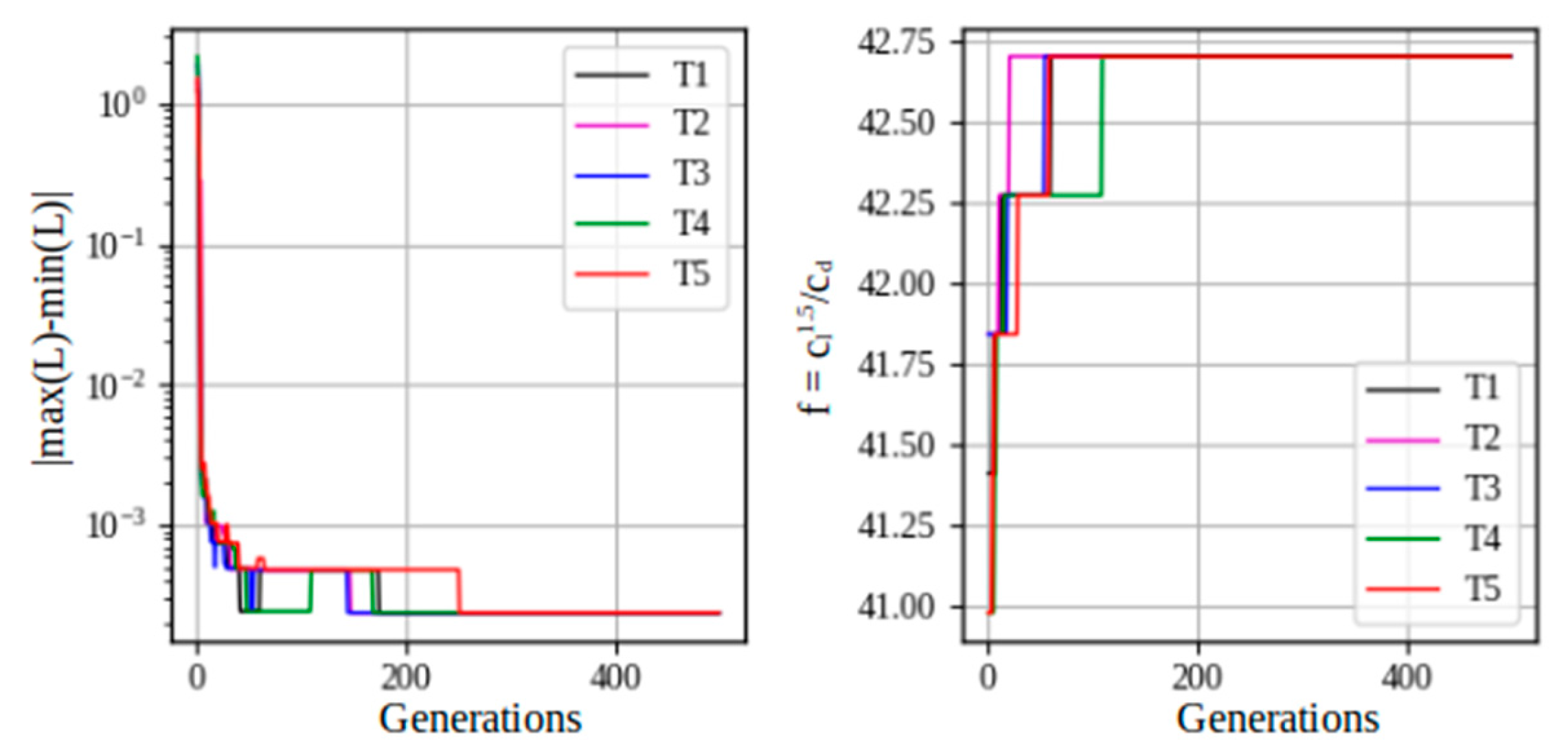
Figure 29.
Optimal airfoils obtained in different tests.
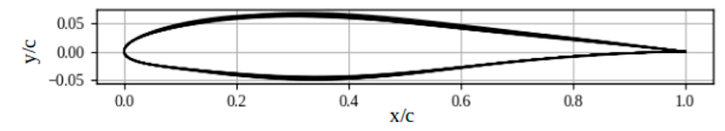
Figure 30.
Optimal airfoils with maximum and minimum ytmax.
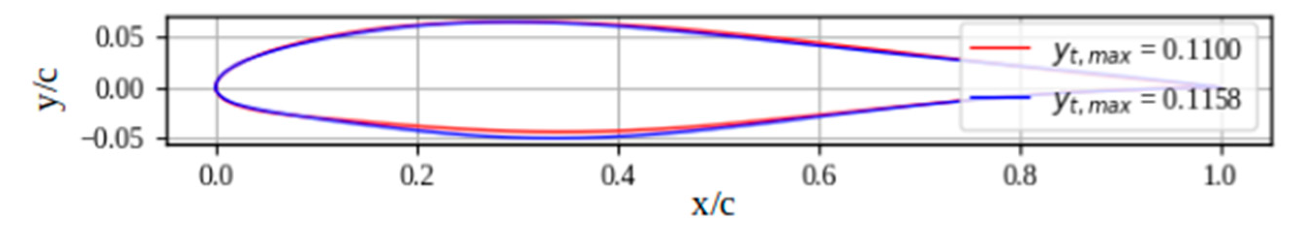
Figure 31.
Evolution of the Pareto front of the 5 optimization tests.
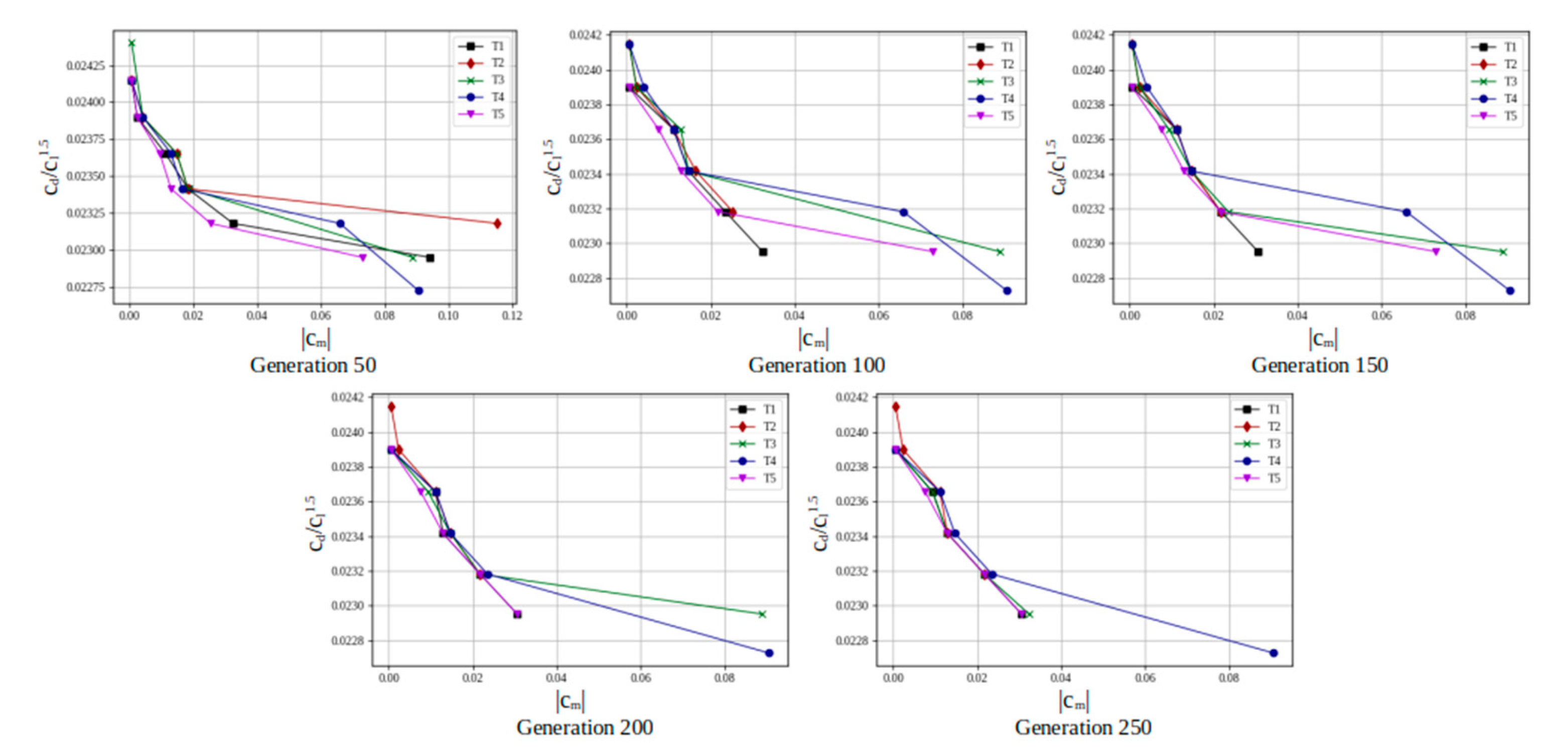
Figure 32.
Best Pareto front obtained in the tests.
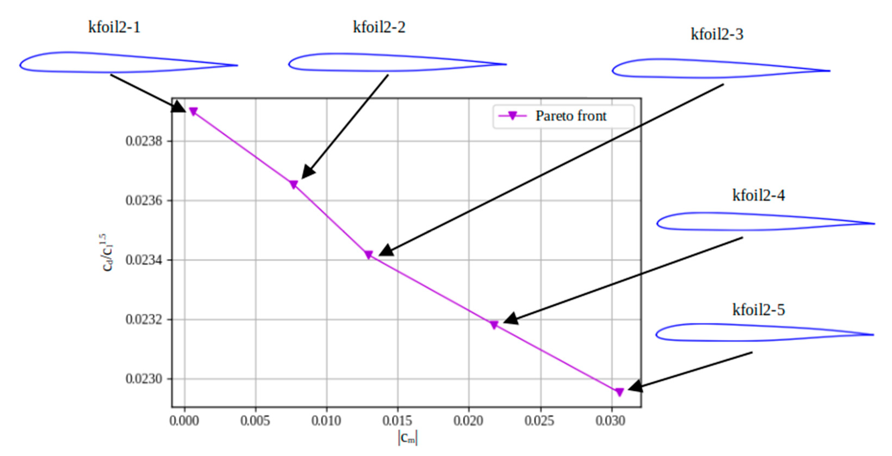
Figure 33.
Comparison of the geometries of the Pareto front profiles.
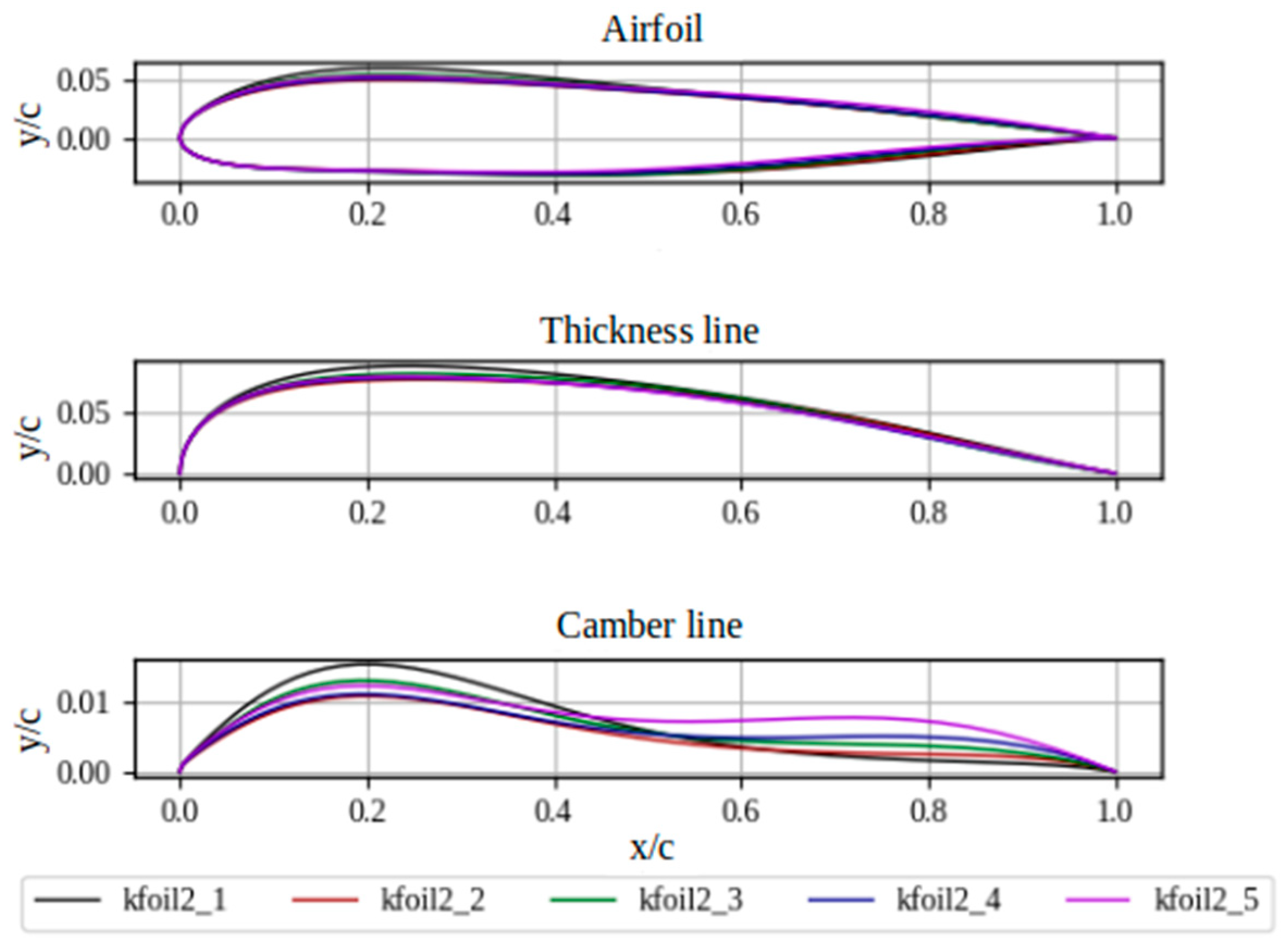
Figure 34.
Aerodynamic comparison of the Pareto front airfoils.
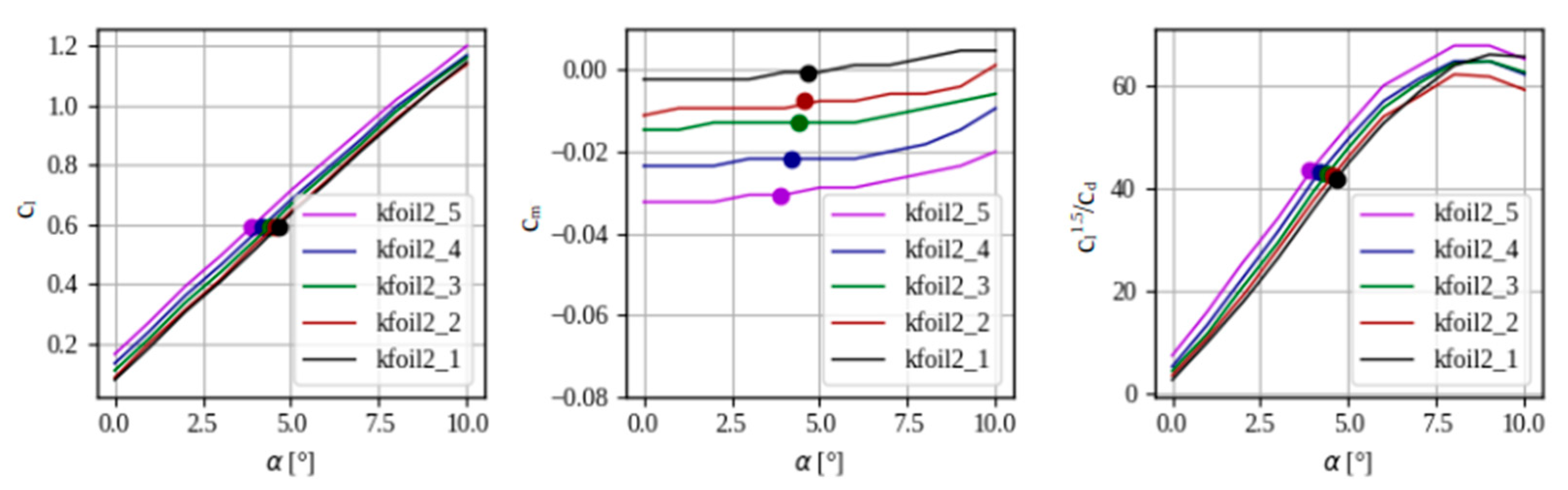

Table 1.
Initial conditions.
| airfoil | inlet | outlet | frontBack | internalField | |
|---|---|---|---|---|---|
| U [m/s] | noSlip | U∞ | U∞ | empty | U∞ |
| p [m2/s2] | zeroGradient | zeroGradient | 0 | empty | 0 |
| k [m2/s2] | kqRWallFunction(k0) | k0 | k0 | empty | k0 |
| ω [1/s] | omegaWallFunction(ω0) | ω0 | ω0 | empty | ω0 |
| νt [m2/s] | nutUWallFunction(0) | 0 | 0 | empty | 0 |
| Type of scheme | OpenFOAM scheme |
|---|---|
| Temporary derivatives | steadyState |
| Gradients | Gauss linear |
| Divergence(φ, U) | bounded Gauss linearUpwind limited |
| Divergence(φ, k) | bounded Gauss upwind |
| Divergence(φ, ω) | bounded Gauss upwind |
| Laplacians | Gauss linear corrected |
| Interpolation | linear |
φ denotes the (volumetric) flux of velocity on the cell faces for constant-density flows, for example Divergence(φ, U) indicates the advection of velocity.
Table 3.
Design intervals of the parameters of the CST method.
| Parameter | Design interval | Parameter | Design interval |
|---|---|---|---|
| Au,0 | [0,07, 0,35] | Al,0 | [-0,30, -0,05] |
| Au,1 | [0,04, 0,55] | Al,1 | [-0,26, 0,05] |
| Au,2 | [0,00, 0,45] | Al,2 | [-0,36, 0,05] |
| Au,3 | [0,00, 0,55] | Al,3 | [-0,47, 0,05] |
| Au,4 | [0,00, 0,55] | Al,4 | [-0,47, 0,05] |
| Au,5 | [0,00, 0,50] | Al,5 | [-0,42, 0,10] |
| Au,6 | [-0,01, 0,50] | Al,6 | [-0,28, 0,10] |
Table 4.
Design intervals of the parameters of the Bezier-PARSEC method.
| Parameter | Design interval | Parameter | Design interval |
|---|---|---|---|
| rle | [-0.030, -0.001] | γle | [-0,01, 0,32] |
| xt | [0,23, 0,50] | xc | [0,20, 0,85] |
| yt | [0,030, 0,095] | yc | [0,010, 0,065] |
| kt | [-0.9, -0.2] | kc | [-1,000, 0,025] |
| βte | [0,01, 0,40] | αte | [0,01, 0,70] |
Table 5.
Generator (G).
| Layer | Number of neurons | Activation function |
|---|---|---|
| Input layer, IL | 5 | ————————— |
| Hidden layer 1, HL1 | 16 | Leaky RELU |
| Hidden layer 2, HL2 | 32 | Leaky RELU |
| Output layer, OL | 14 | Hyperbolic tangent |
Table 6.
Discriminator (D).
| Layer | Number of neurons | Activation function |
|---|---|---|
| Input layer, IL | 14 | ————————— |
| Hidden layer 1, HL1 | 32 | Leaky RELU |
| Hidden layer 2, HL2 | 16 | Leaky RELU |
| Output layer, OL | 1 | Sigmoid |
Table 7.
Characteristics of the simulated flows in the NACA 0012 airfoil.
| Test | M [Re] |
|---|---|
| 1 | 0.15 [2x10⁶] |
| 2 | 0.15 [4x10⁶] |
| 3 | 0.15 [6x10⁶] |
| 4 | 0.30 [4x10⁶] |
| 5 | 0.30 [6x10⁶] |
Table 8.
Average values of MAE in the reconstruction of graphs in the VAE testing stage.
| Size of z | MAE | MAEavg | ||
|---|---|---|---|---|
| cl1.5/cd | cm | cl | ||
| 9 | 0.00291 | 0.00218 | 0.00196 | 0.00235 |
| 8 | 0.00283 | 0.00220 | 0.00165 | 0.00223 |
| 7 | 0.00281 | 0.00223 | 0.00185 | 0.00223 |
| 6 | 0.00294 | 0.00203 | 0.00199 | 0.00232 |
| 5 | 0.00341 | 0.00331 | 0.00212 | 0.00294 |
Table 9.
Parameters and their design ranges to optimize MLP hyperparameters.
| η | Design ranges |
|---|---|
| n1 | [128; 512] |
| n2 | |
| n3 | |
| a1 | {0; 1; 2}* |
| a2 | |
| a3 |
*0 - hyperbolic tangent, 1 – RELU, 2 – Leaky RELU.
Table 10.
Repeatability analysis of the obtained values obtained by the optimization algorithm.
| NP0 | Test | cl1.5/cd | α [°] | ytmax | cd | cm |
|---|---|---|---|---|---|---|
|
10|ξ| |
1 | 42.7059 | 3.9 | 0.1127 | 0.0106 | -0.0342 |
| 2 | 42.7059 | 3.9 | 0.1102 | 0.0106 | -0.0342 | |
| 3 | 42.7059 | 3.9 | 0.1136 | 0.0106 | -0.0323 | |
| 4 | 42.2745 | 3.9 | 0.1148 | 0.0107 | -0.0342 | |
| 5 | 42.7059 | 3.9 | 0.1100 | 0.0106 | -0.0323 | |
|
20|ξ| |
1 | 42.7059 | 3.9 | 0.1148 | 0.0106 | -0.0341 |
| 2 | 42.7059 | 3.9 | 0.1136 | 0.0106 | -0.0376 | |
| 3 | 42.7059 | 3.9 | 0.1117 | 0.0106 | -0.0341 | |
| 4 | 42.7059 | 3.9 | 0.1118 | 0.0106 | -0.0341 | |
| 5 | 42.7059 | 3.9 | 0.1122 | 0.0106 | -0.0341 | |
|
50|ξ| |
1 | 42.7059 | 3.9 | 0.1158 | 0.0106 | -0.0341 |
| 2 | 42.7059 | 3.9 | 0.1117 | 0.0106 | -0.0341 | |
| 3 | 42.7059 | 3.9 | 0.1113 | 0.0106 | -0.0359 | |
| 4 | 42.7059 | 3.9 | 0.1127 | 0.0106 | -0.0341 | |
| 5 | 42.7059 | 3.9 | 0.1104 | 0.0106 | -0.0359 |
Table 11.
Comparison of the aerodynamic coefficients of optimal profiles obtained using OpenFOAM and AZTLI-NN.
Table 11.
Comparison of the aerodynamic coefficients of optimal profiles obtained using OpenFOAM and AZTLI-NN.
| Airfoil | Method | α [°] | cl | cd | cm | cl1.5/cd | yt,max |
|---|---|---|---|---|---|---|---|
| Kfoil_1 | OpenFOAM | 3,9 | 0,5847 | 0,0109 | -0,0293 | 41,0178 | 0,1100 |
| Kfoil_1 | AZTLI-NN | 3,9 | 0,59 | 0,0106 | -0,0323 | 42,7059 | 0,1100 |
| Kfoil_2 | OpenFOAM | 3,9 | 0,5801 | 0,0110 | -0,0303 | 40,1662 | 0,1158 |
| Kfoil_2 | AZTLI-NN | 3,9 | 0,59 | 0,0106 | -0,0341 | 42,7059 | 0,1158 |
Table 12.
Aerodynamic characteristics of the Pareto front profiles under the condition of design.
| Airfoil | α [°] | cl | cd | cm | cl1,5/cd | yс,max | yt,max |
|---|---|---|---|---|---|---|---|
| kfoil2_1 | 4,6 | 0,5900 0,5933* | 0,0109 0,0110* | -0,0006 -0,0029* | 41,5431 41,5450* | 0,0154 | 0,0888 |
| kfoil2_2 | 4,5 | 0,5900 0,5907* | 0,0107 0,0108* | -0,0079 -0,0117* | 42,2745 42,0365* | 0,0108 | 0,0776 |
| kfoil2_3 | 4,3 | 0,5900 0,5905* | 0,0106 0,0107* | -0,0129 -0,0150* | 42,7059 42,4078* | 0,0130 | 0,0823 |
| kfoil2_4 | 4,1 | 0,5900 0,5878* | 0,0105 0,0107 | -0,0218 -0,0231* | 43,1373 42,5146* | 0,0111 | 0,0791 |
| kfoil2_5 | 3,9 | 0,5900 0,5930* | 0,0104 0,0106* | -0,0305 -0,0303* | 43,5686 43,0800* | 0,0123 | 0,0800 |
*values obtained using OpenFOAM.
Disclaimer/Publisher’s Note: The statements, opinions and data contained in all publications are solely those of the individual author(s) and contributor(s) and not of MDPI and/or the editor(s). MDPI and/or the editor(s) disclaim responsibility for any injury to people or property resulting from any ideas, methods, instructions or products referred to in the content. |
© 2024 by the authors. Licensee MDPI, Basel, Switzerland. This article is an open access article distributed under the terms and conditions of the Creative Commons Attribution (CC BY) license (http://creativecommons.org/licenses/by/4.0/).
Copyright: This open access article is published under a Creative Commons CC BY 4.0 license, which permit the free download, distribution, and reuse, provided that the author and preprint are cited in any reuse.


