
Submitted:
09 July 2024
Posted:
10 July 2024
You are already at the latest version
Abstract
In transient phase of an atmospheric-pressure discharge, the avalanche turns into a streamer discharge with time. Hydrodynamic fluid models are frequently used to describe the formation and propagation of streamers, where charge particle transport is dominated by the creation of space charge. The required electron transport data and rate coefficients for the fluid model are parameterized using the local mean-energy approximation (LMEA) and the local field approximation (LFA). In atmospheric pressure applications, the excited species produced in the electrical discharge determine the subsequent conversion chemistry. We performed the fluid model simulation of streamers in nitrogen gas at atmospheric pressure using three different parametrizations for transport and electron excitation rate data. We present the spatial and temporal development of several macroscopic properties such as electron density and energy, and the electric field during the transient phase. The species production efficiency which is important to understand the efficacy of any application of non-thermal plasmas is also obtained for the three different parametrizations. Our results suggest that at atmospheric pressure all three schemes predicted essentially the same macroscopic properties. Therefore, a lower order method such as LFA which does not require the solution of the energy conservation equation should be adequate to determine the streamer macroscopic properties to inform most plasma-assisted applications of nitrogen containing gases at atmospheric pressure.
Keywords:
fluid models
; local mean energy approximation
; local field approximation
; streamers
; non-thermal plasma
; space charge dominated transport
1. Introduction
The development of an electrical discharge and the subsequent plasma formation is strongly dependent on the operating pressure and gas composition. Non-thermal plasmas, including low-pressure DC glows, RF discharges, and atmospheric pressure discharges have, many applications and serve as enabling technology in critical manufacturing processes [1,2,3,4,5]. The transient phase of an atmospheric-pressure discharge consists of an avalanche which leads to the streamer phase. If left uninterrupted, it will eventually lead to an arc formation [6]. In most applications the discharge is terminated: In repetitive nano-second pulse discharges, the pulse widths are short enough to avoid arc formation and in dielectric-barrier discharges the charging of the dielectric quenches the micro discharge. From the perspective of plasma chemistry applications in such diverse areas such as plasma medicine to plasma-assisted combustion, the understanding of the reactive species production during the streamer phase is important [7,8]. The applications of nonthermal plasmas are based on the production of excited species, photo emission and reactive radicals at or near ambient temperature [9,10,11,12]. These types of plasma are partially ionized gases where the free electrons and heavy ions gain energy from the electric field and undergo elastic or inelastic collision with background particles or wall leading to energy loss. Due to the large difference in the mass ratio, most of the energy gain from the field is by electron transport across potential gradients. In certain applications with changing environment a computationally efficient model for the streamer development will help the implementation of complex plasma chemistry phenomenon such as plasma-assisted combustion [7].
Nonthermal plasmas can reach a steady state in discharges, such as low-pressure DC glows or radio-frequency discharges, and others are transient discharges, such as an atmospheric pressure streamer discharge. Near atmospheric pressure, electrical discharges produce spatially and temporally varying space charge which substantially alter the applied electric field and impose constraints on models. Non-local electron kinetics play an important role in low pressure capacitively coupled rf discharge and low-pressure DC glows. We are particularly interested in studying the breakdown of atmospheric pressure gases. The non-thermal or cold plasmas at atmospheric pressure forms the basis for many applications including manufacturing, plasma medicine, disinfection etc. [1,2,12].
The streamer mechanism was first proposed by Raether [13] and Leob and Meek [14] to explain electrical breakdown at high pressures. Since then, a large number of both experimental and numerical studies have resulted in a better understanding of its formation and propagation [15,16,17,18,19,20,21,22,23]. Theoretical efforts are constrained by the fact that the mathematical description of space-charge dominated transport is difficult to deal with because of the sharp density and field gradients. Most approaches to the modeling of streamers can be lumped under kinetic or fluid approach. In kinetic models the Boltzmann equation coupled with Poisson equation is solved for the phase space of electrons. Alternately, Monte Carlo simulations with detailed particle transport using collisional cross-sections is used to determine the particle phase space. To cover the full six-dimensional phase space is computationally expensive, and this approach has found very little use in general. A computationally tractable hybrid approach is the Particle-in-cell Monte Carlo simulations (PIC-MCC) where a large number of electrons are followed in the phase-space using Monte Carlo techniques used to simulate collisions, and the electric field is obtained from the solution of Poisson’s equation from the charged particle densities lumped in an appropriate mesh [21]. The 3-D PIC-MCC have been particularly successful in modeling stochastic fluctuations leading to branching of streamers observed experimentally [18]. Several articles have been published to understand the validity of the modeling approach for plasma fluid models: Nijdam et al. have reported numerical modeling including the pros and cons of particle-in-cell (PIC) and fluid models [19]. Kim et al. benchmarked PIC, fluid, and hybrids models by comparing simulation results with experimental results for plasma displays, capacitively coupled plasma and inductively coupled plasma. They concluded that despite progress in modeling and simulation of low-temperature plasma, these models still need improvements [20].
In plasma fluid models the plasma hydrodynamics is described by macroscopic quantities such as electron density, drift velocity, and mean electron energy. The fluid models can be theoretically constructed by taking the velocity/energy moments of the Boltzmann equation. The first three moments gives the particle, momentum, and energy conservation equations to describe the plasma hydrodynamics and depending on the number of moments considered, appropriate closure approximations are required. The first order drift-diffusion model based on local field approximation (LFA) has been used with some success in predicting and reproducing experimental results of the formation and propagation of streamer channels [15,16,17,18,19,20,21,22,23]. It has been reported that the assumption of local equilibrium of the electron energy deviates significantly at the fast-changing ionization fronts with steep density and field gradients [19]. In the hydrodynamic description of non-thermal plasma, the electron transport and collisional rate coefficients are commonly parameterized by the local-field or the local mean-energy. For most commonly used gases, the transport and collision rates can be readily obtained from the two-term solution of the Boltzmann equation from electron impact cross-section data [24,25].
Second order drift-diffusion model considers electron energy transport where the parameters are based on local mean energy approximation (LMEA) and several reports concluded that this model gives better results at streamer fronts. Luque and Ebert reviewed density models for streamer discharge simulation, detailing their physical foundation, their range of validity and the most relevant algorithm employed in solving them [21]. Markosyan et al. compared plasma fluid models for one-dimensional streamer ionization fronts and compared it to PIC model 22]. They found the local energy approximation and a higher order model were in better agreement with the PIC simulations, and the local field approximation gave reasonably close results. Gruber et al. examined the local field and local energy models for simulation of low-pressure DC glow and capacitively coupled rf discharges at low pressures (10 and 100 Pa) in argon and oxygen. They concluded that the LFA method is not recommended for the gas discharge modeling in general at this pressure due to the inadequacy of the drift-diffusion approximation and their results should be checked against experimental data or benchmark approaches [23].
We are interested in examining the plasma fluid models which would be suitable for investigating streamers near atmospheric pressures under ambient conditions. Although several publications have investigated this question, there are results on the impact of the fluid model parametrization on excited species production. Our approach is not so much to replicate experimental results or streamer branching but come up with a suitable model to predict the important characteristics of a streamer that can inform modeling of applications such as plasma medicine and plasma-assisted combustion. The purpose of the current paper is to understand under what condition is the local field approximation and the local mean energy approximation a valid parameter for the transport and rate coefficients. In this paper we simulate the streamer development and propagation in nitrogen by using three different parametrization scheme and compare the important characteristics such as excited species generation. Most applications are under ambient conditions; therefore, study of nitrogen gas can serve as a good model.
2. Fluid Models for Streamer Discharges
During the transient phase the heavy particles do not gain energy in the short period and the neutral gas and ion are at or near room temperature. Also, in the time scale of interest (few ns) the ions can be considered to be stationary compared to the lighter electrons. Both the first order and the second order fluid models for a non-attaching gas include the following particle conservation equations. In the first order model, the parameter is the local reduced electric field, E/N, and in the second order model it is the local mean electron energy, ε. [15,22]
The quantity S represents various ion/electron source or sink mechanisms such as photoionization, recombination, attachment or remnant space charge in repetitive discharges. In the absence of magnetic field and assuming the velocity of the electrons is large compared to the slow species and the plasma is isothermal, the particle flux can be obtained from the momentum conservation equation and is given by [15,19]
where ne and ni are the electron and positive ion density respectively, µe is the electron mobility, De is electron diffusion coefficient, and νI is the ionization frequency. In slowly varying electric field where the magnetic field can be neglected the electric field E is obtained from the solution of the Poisson equation [15].
where qe is the unsigned electron charge and is the free space permittivity. In the second order fluid model, the mean electron energy, ε, is determined from the energy conservation equation [22].
where and are the electron energy dependent collision rate coefficient and energy loss per electron per collision for the jth collision process. The first term in the right-hand side of equation 5 is the convective term and second term is the energy gained from the electric field and third term is the energy loss due to inelastic collisions. This term can also be determined from the energy mobility and diffusion, if known, instead of assuming the 5/3 factor when using the electron transport parameters. A later part of this paper examines the contribution of each of these terms to the time evolution of the electron energy.
In streamer discharges the ionization front propagates at speeds several times higher than the local drift velocity and experience steep spatial gradients due to rapid growth of ionization. It has been suggested that the first order model is not adequate to describe the formation and propagation of these discharges, and a second order model which calculates the local mean energy should be used [23]. Local mean energy can then be used as a parameter to estimate the transport parameters and rate coefficients.
In this article three different parametrizations shown in Table 1 are investigated to understand the differences between the schemes in predicting streamer characteristics. The LMEA and the hybrid methods require the solution of the energy conservation equation. We introduce a new parameterization scheme (hybrid) where the mobility and diffusion are determined from the local electric field which is readily available and the electron-impact rates such as ionization and excitation from the local electron energy. The justification for proposing this scheme is from a previous set of studies that show that the electron drift tracks the local electric field more closely compared to the electron energy [24].
3. Results and Discussion
The simulations were done in two-dimensions with azimuthal symmetry. The transport parameters and rate coefficients were determined using the open-source Boltzmann solver, BOLSIG+, with Lxcat nitrogen cross sections [25,26]. The Boltzmann solver solves for the electron energy distribution function for a given reduced electric field (E/N) which also provides the corresponding electron energy. The transport coefficients and rates can then be parameterized with either the reduced field or the electron energy.
The discharge consists of a gap of 5 mm filled with atmospheric pressure nitrogen. The results presented here is for an applied step voltage of (186 Td) which resulted in an anode directed streamer. The set of equation 1-5 was solved numerically using finite difference method. The boundary conditions for particles at the electrodes were set to inflows or sinking of particles without creating an electrode sheath. A more physical boundary condition would require detailed knowledge of the electrode. In such discharges, the cathode sheath has very little impact on the bulk properties of the streamer. The Flux-Corrected Transport (FCT) method proposed by Boris and Book was used for the convective term of both the electron density and electron energy equations [27,28]. This method is particularly suitable for handling the steep density and field gradients encountered in streamer propagation. A uniform grid spacing of 500 is used both in the z and r directions giving a spatial resolution of 10 μm. The details of the method as applied to streamers have been expensively reported [15,16,17].
The following boundary conditions were used for the solution of the Poisson’ equation.
The Poisson’s equation is solved for the electric potential by Successive Over relaxation (SOR) method [29]. This is an iterative method and converges rapidly as there is small perturbation from the previous time step. For our simulation a relaxation factor ω=1.9475 gave the fastest convergence. The maximum relative error at any grid point was set to 10-5 for the convergence criterion.
The results presented here are for anode directed streamers. The results were very similar for cathode-directed streamers. In order to bypass the avalanche phase, an initial neutral plasma is placed at the cathode which represents the space charge formed. Details of this method and the background seeding of electrons to represent ionization can be found in references 15 and 16. Figure 1, Figure 2 and Figure 3 show the contour plots electron density, electron energy, and electric field contours at different times for the fluid model with hybrid parametrization. These plots are typical of steamer propagation where the streamer tip shows high gradients for electron density, electron energy and electric field. In the streamer bulk, away from the tip, the electron energy and electric field is fairly constant.
The three different type of parametrization results in similar contours plots. For comparison, the on-axis density, and the electric field are plotted for streamer formation using the three different parametrizations at nearly equal time and are shown in Figure 4 and Figure 5 respectively. Since the time steps for the simulation is determined from the current Courant–Friedrichs–Lewy criteria, the comparison plots are not exactly at the same instant [30]. The electron density and the electric field as determined from three different parametrization give very similar results with only minor difference which has very little impact in the development and propagation of the streamer.
The streamer speed as a function of time is shown in Figure 6 for the three different parametrizations. Again, we see very little difference in the speed irrespective of the method used for solving the fluid equations. The speed of the ionization front increases with time as the field enhancement at the tip of the streamer also increases with time as the streamer propagates. Higher the field enhancement, the quicker is the plasma density build-up due to electron impact ionization. The magnitude of the velocities of streamer in nitrogen is close to experimentally reported values: Wagner reported an anode directed velocity 0.4x10⁶ m/s at 156 Td in atmospheric pressure nitrogen and Chalmers et al. reported an anode directed velocity 0.1 to 0.4 x 10⁶ m/s in the range of 126 to156 Td [31,32].
The spatial and temporal evolution of the energy obtained from the solution of the energy equation was compared to the energy predicted by the local electric field using the equilibrium relationship between the reduced electric field (E/N) in Td and electron energy, in nitrogen as obtained from the solution of the Boltzmann equation shown below.
The axial plot of the energy for the three different parameterization is shown in Figure 7, Figure 8 and Figure 9 for the LFA, hybrid, and LMEA respectively. Remarkably for all three parametrization the electron energy agrees very well with local electric field prediction at the streamer tip where the density and field gradients are the highest. There is a slight difference in the bulk of the streamer due to slight electron cooling predicted by energy equation which is discussed in a later section.
Since in most applications where streamer type discharges are used to generate excited species, an estimation of the species concentration is important in determining subsequent plasma chemical pathways. Shown in Figure 10 is the G-factor, which is the number of radicals produced per 100 eV of electrical energy input, for three of the nitrogen excited states , ,and [32]. The three model parametrizations predict very similar G-factors which remains fairly constant with time. The current increases with time as the streamer propagate along the axial direction. Therefore, the electrical energy input increases with time and radical densities increase with time although the G-factor don’t change with time.
The contribution to the energy change at spatial points along the axis was studied by looking at the first term on the right-hand side of the energy conservation equation which is the convective term and the net energy gain which is the sum of the second (energy gained form the electric field) and the third (energy lost due to inelastic process). The energy gain from the electric field and the inelastic loss are almost equal and an order of magnitude higher than the convective contribution. Figure 11 shows the relative contribution of due to convective term, gain-loss term, and the net energy density rate for the hybrid and LMEA parametrizations. The LFA is not shown because the energy equation is not relevant to that method. At the streamer tip there is a net transport of electron energy due to convection from the back to the front due to electron transport. The net effect is very similar in both parametrization and there is a net cooling behind the streamer tip. This cooling effect is seen in the energy plots (Figure 7, Figure 8 and Figure 9) where the energy in the bulk shows a slight decline further away from the cathode.
Our results suggest that the electron energy in a nitrogen streamer at atmospheric pressure quickly reaches equilibrium with the electric field and the convective transport of energy does not have a significant impact. The various characteristics of the streamer discussed here show very little dependence on the parameterization. Markosyan et al. have done similar studies in 1-D streamer model. They compared different fluid model with a 1-D PIC simulation. Although the 1-D models have inherent shortcomings due to the gross simplification in estimating the spatial profile of the electric field, there findings are similar to what we observe in our simulations. A similar conclusion was reached by Wang et al, where they looked at particle and fluid models for streamer discharges in air [33]. Li et al. looked at the deviations from the LFA in negative streamer heads in nitrogen streamer head when compared to particle models. They conclude that the largest discrepancy is in the leading edge of the front where the electron density is very low and electric field is not screened [34]. As such this result will have minimum impact on estimating the overall radical generation in a streamer discharge. Our work confirms the choice of parametrization has very little impact on the species generation in the discharges studied.
4. Conclusion
At or near atmospheric pressure, the space charge dominated transport of the streamer mechanism of transient electrical breakdown of nitrogen was investigated using fluid models with three different parametrization schemes. These included the commonly known LEA and LMEA and a hybrid parametrization scheme in which the drift and diffusion is determined from the local reduced electric field and the electron impact rates are determined from the local electron energy. Several important characteristics of the streamer were reported including electron density, electric field, electron energy, streamer velocity, and excited species production efficiency. These properties showed very little dependence on the parametrization scheme. We conclude that using a second order method such as LMEA does not provide any additional advantage for high pressure discharges in gases such as air containing molecular gases like nitrogen even in the presence of very steep density and field gradients. Our results suggest that the electron energy reach local equilibrium and the convective energy transport has minimal impact on the overall electron energy. This conclusion is significant in developing efficient codes if the solution of the energy equation is required. For applications where repeated streamer simulation is required due to changing environment this would save considerable amount of computation time. It remains to be seen if this would apply for predominantly atomic gases which have significantly different electron energy dependence on E/N due to the absence of energy loss to vibrational excitation.
Data Availability
The data that support the findings of this study are openly available in reference number Refs. 25 and 26.
Acknowledgments
This work was partially supported by the US Office of Naval Research (Grant Number: W911NF-23-1-0173) and the National Science Foundation (Award Number: 2337461).
References
- Kogelschatz U, 2003, Plasma Chemistry and Plasma Processing, 23, 1.
- Weltmann K D, Kolb J. F, Holub M, Uhrlandt D, Simek M, Ostrikov K, Hamaguchi S, Cvelbar U, Cernak M, Locke B, Fridman A, Favia P, and Becker K, 2009, Plasma Process Polym., 16 e1800118.
- Li J, Wanming S, Pashaie B, and Dhali S K, 1995, IEEE Tran. Plasma Science, 23, 672.
- Marode E, Goldman A, and Goldman M, Non-thermal plasma techniques for pollution control, Part A: Overview, 1993 Fundamentals and Supporting Technologies, Edited by B. M. Penetrante and S. E. Schultheis, NATO ASI Series, Springer-Verlag, p167.
- Dhali S K, 2021, AIP Advances 11, 015247.
- Ganesh S, Rajabooshanam A, Dhali S. K., 1992, Journal of Applied Physics, 72, 9.
- Adamovich I V and Lempert, W R,2015, Plasma Phys. Control. Fusion, 57, 01400.
- Lu, X P, Reuter, S, Laroussi M, and Liu, D W,2019, Nonequilibrium Atmospheric Pressure Plasma Jets: Fundamentals, Diagnostics, and Medical Applications. CRC Press ISBN 978-0-429-62072-0. .
- Dhali S K, 2020, AIP Advances, 10, 035002.
- Sankaranarayan R, Pashaie B and Dhali S K, 2000, Appl. Phys. Lett., 77, 2970.
- Shakir S, Mynampati S, Pashaie B and Dhali S K, 2006, J. Appl. Phys., 99, 073303.
- Bruggeman J P, Iza F, and Brandenburg R, 2017, Plasma Sources Sci. Technol. 26 123002.
- Raether H, 1939, Z. Phys. Vol. 112, p464; Arch. Electrotech., 1940, 34, p49.
- Loeb J B and Meek J M, 1940, J. Appl. Phys., 11, 438.
- Dhali S K and Williams P F, 1987, J. Appl. Phys., 62, 4696.
- Dhali S K and Pal A K, 1987, J. Appl. Phys., 63.
- Morrow R, 1985, Phys. Rev. A. 32, 1799.
- Teunissen J, and Ebert U, 2016, Plasma Sources Sci. Technol. 26, 044005.
- Nijdam S, Teunissen J, and Ebert U, 2020, Plasma Sources Sci. Technol., 29, 103001.
- Kim H C, Iza F, Yang S S, Radmilovic-Radjenovic M, and Lee J K, 2005, J. Phys. D: Appl. Phys. 38, R283-R301.
- Luque A and Ebert U, 2012, Journal of Computational Physics, 231, 904.
- Markosyan A H, Teunissen J, Dujko S, and Ebert U, 2015, Plasma Sources Sci. Technol. 24 065002.
- Grubert G K, Becker M M, and Loffhagen D, 2009, Phys. Rev. E, 80, 036405.
- Dhali SK,2022, Plasma Sources Sci. Technol. 31. [CrossRef]
- Phelps database, www.lxcat.net, retrieved on December 30, 2020.
- Hagelaar G J M, and Pitchford L C, 2005, Plasma Source Science and Technology, 14, 722.
- Zalesak S T, 1979, J. Computational Physics, 31, 335.
- Boris J P and Book D L, 1973, Computational Physics, 11, 39.
- Li J, Sun W, Pashaie B, and Dhali S K, (1995), IEEE Transactions on Plasma Science, 23, 4. [CrossRef]
- Courant R, Friedrichs K, Lewy H, 1967, IBM Journal of Research and Development. [CrossRef]
- Wagner K H, 1967, Z. Phys. 204.
- Lofthus A, Krupenie P H, 1977 Journal of Physical and Chemical reference Data, 6,.1.
- Wang Z, Sun A, Teunissen J (2021) Plasma Sources Sci. Technol. 31.
- Li C, Brok W J M, Ebert U M, 2007, J. Appl. Physics, 101(2).
Figure 1.
The contour plot of electron density at three different instances in time for nitrogen gas at one atmosphere for an applied voltage of 25 kV across a 5 mm gap. The z distance is from the cathode. The hybrid parametrization was used for the plasma model.
Figure 1.
The contour plot of electron density at three different instances in time for nitrogen gas at one atmosphere for an applied voltage of 25 kV across a 5 mm gap. The z distance is from the cathode. The hybrid parametrization was used for the plasma model.
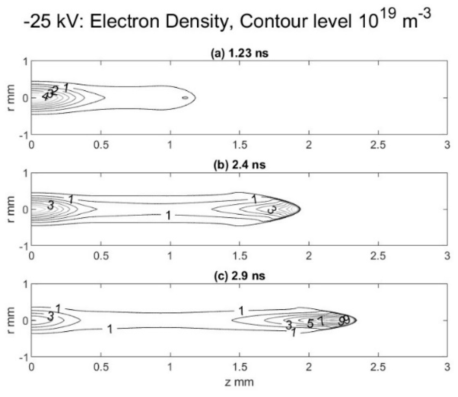
Figure 2.
The contour plots of the axial electric field. All other conditions are the same as Figure 1.
Figure 2.
The contour plots of the axial electric field. All other conditions are the same as Figure 1.
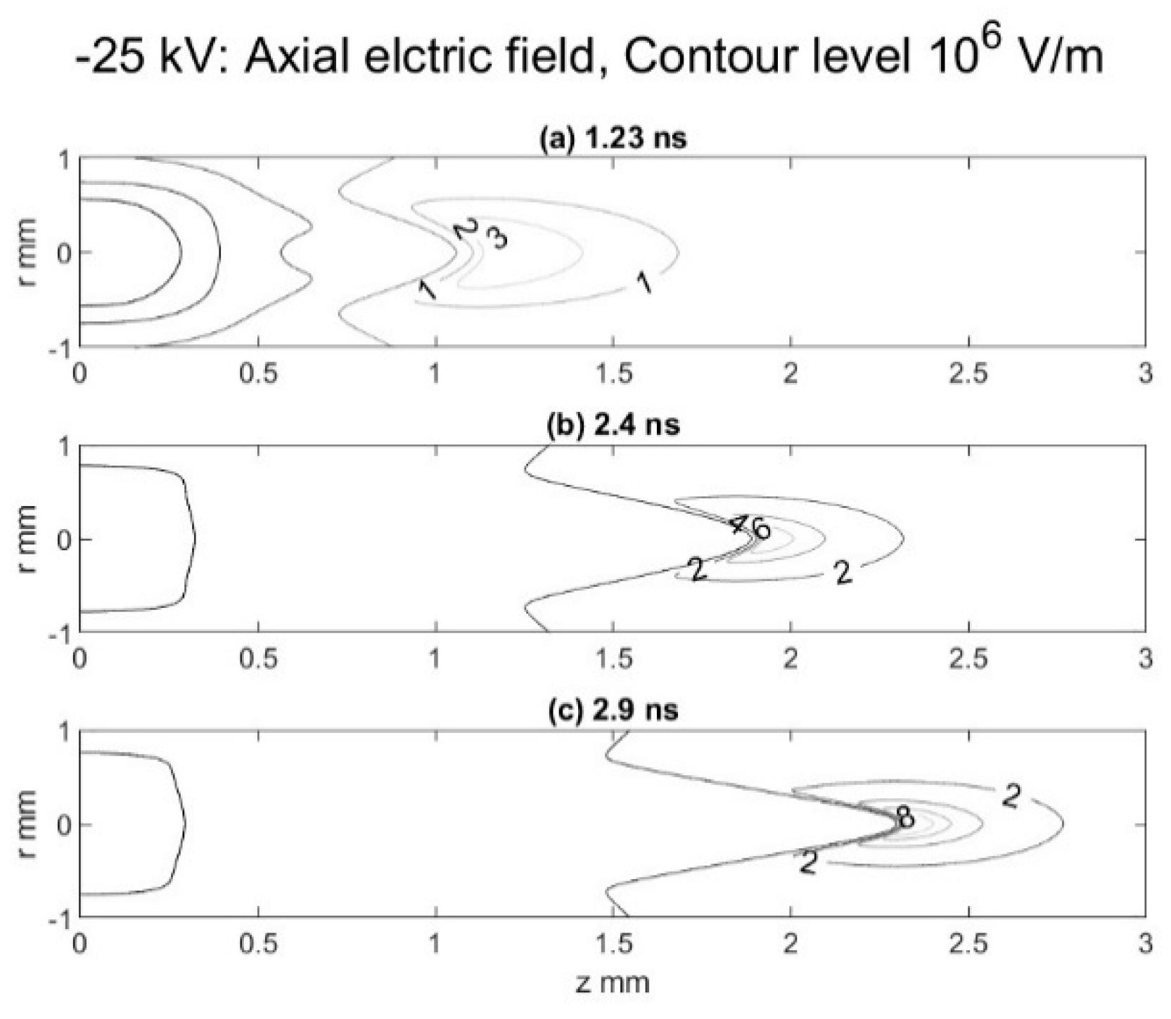
Figure 3.
The on-axis plots of electron energy. All other conditions are the same as Figure 1.
Figure 3.
The on-axis plots of electron energy. All other conditions are the same as Figure 1.
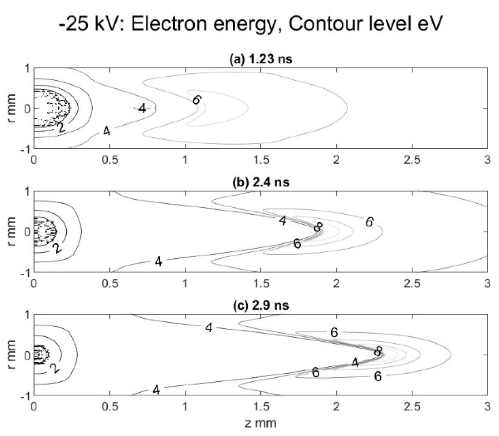
Figure 4.
The axial electron density plots shown as a function of the distance from the cathode. The simulations conditions are the same as in Figure 1.
Figure 4.
The axial electron density plots shown as a function of the distance from the cathode. The simulations conditions are the same as in Figure 1.
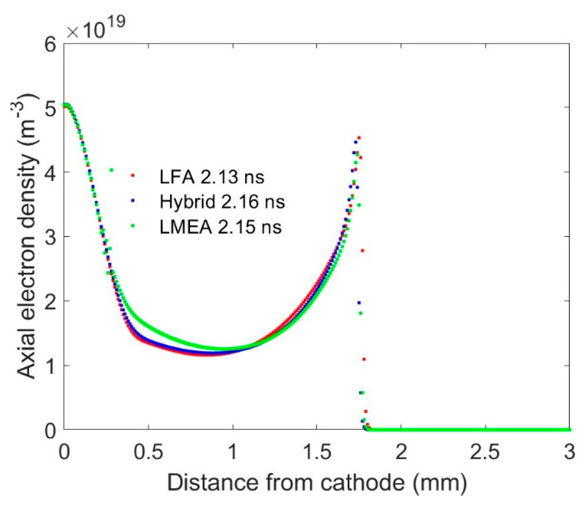
Figure 5.
The on-axis electric field for the three different parametrizations. The simulations conditions are the same as in Figure 1.
Figure 5.
The on-axis electric field for the three different parametrizations. The simulations conditions are the same as in Figure 1.
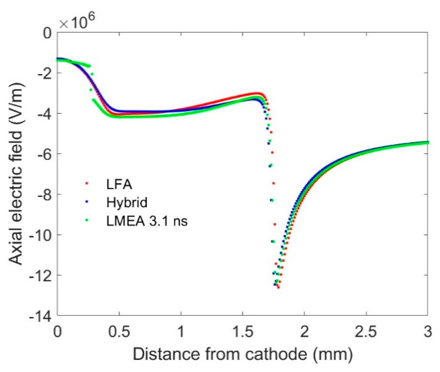
Figure 6.
The streamer speed as a function of time from the start of the pulse for the three different parametrizations considered.
Figure 6.
The streamer speed as a function of time from the start of the pulse for the three different parametrizations considered.
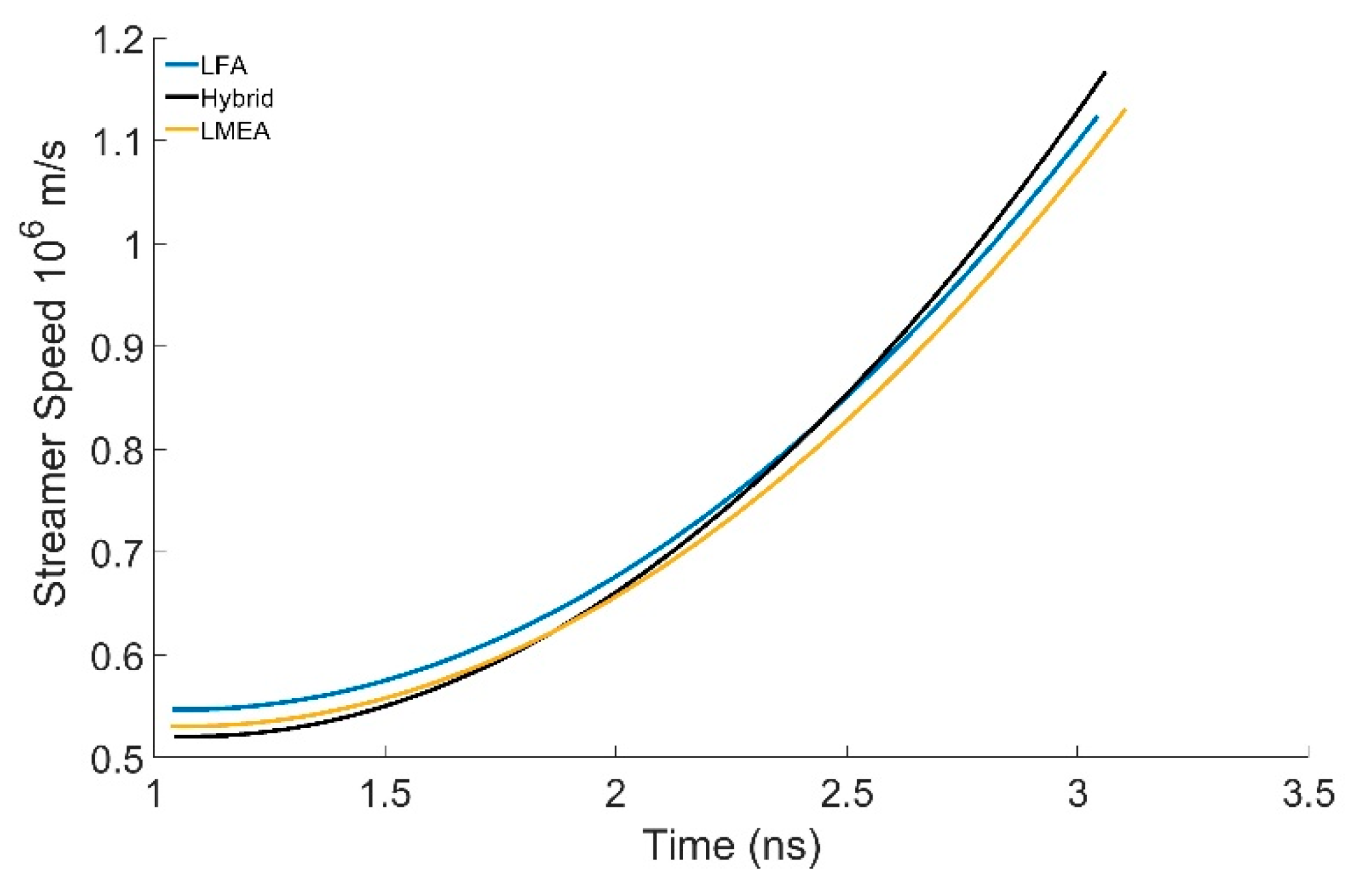
Figure 7.
The on-axis electron energy as a function of the distance from the cathode determined from the energy equation (local energy) and the steady-state local field (equation 7) with LFA parametrization. The simulations conditions are the same as in Figure 1.
Figure 7.
The on-axis electron energy as a function of the distance from the cathode determined from the energy equation (local energy) and the steady-state local field (equation 7) with LFA parametrization. The simulations conditions are the same as in Figure 1.
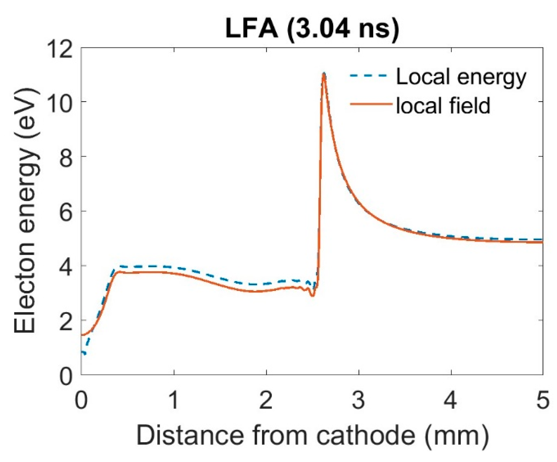
Figure 8.
The on-axis electron energy as a function of the distance from the cathode determined from the energy equation (local energy) and the steady-state local field (equation 7) with hybrid parametrization. The simulations conditions are the same as in Figure 1.
Figure 8.
The on-axis electron energy as a function of the distance from the cathode determined from the energy equation (local energy) and the steady-state local field (equation 7) with hybrid parametrization. The simulations conditions are the same as in Figure 1.
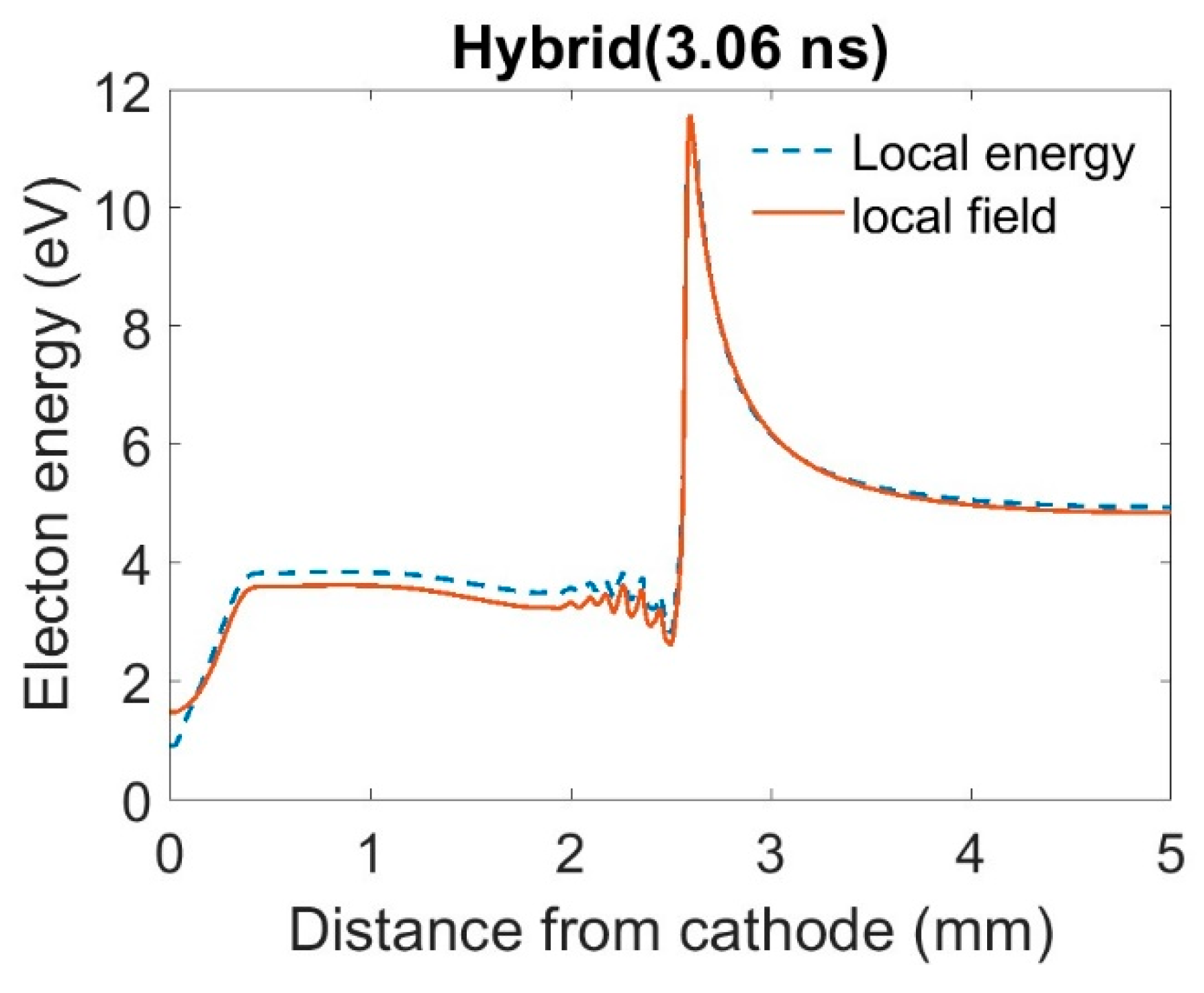
Figure 9.
The on-axis electron energy as a function of the distance from the cathode determined from the energy equation (local energy) and the steady-state local field (equation 7) with LMEA parametrization. The simulations conditions are the same as in figure 1.
Figure 9.
The on-axis electron energy as a function of the distance from the cathode determined from the energy equation (local energy) and the steady-state local field (equation 7) with LMEA parametrization. The simulations conditions are the same as in figure 1.
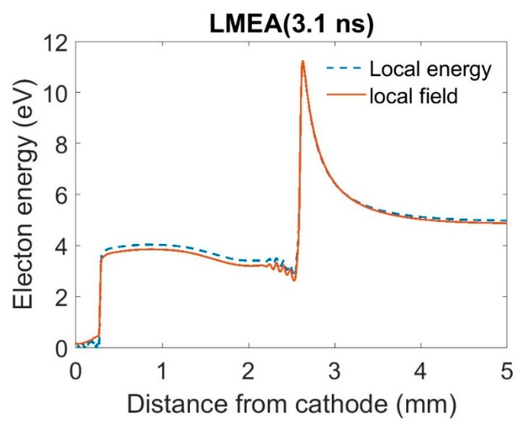
Figure 10.
The G-factor (number of radicals produced per 100 eV of electrical energy) for three different nitrogen excited state as determined by the three different parametrization schemes: The ◊, x, and + correspond to the LFA, hybrid and LMEA respectively, and red, blue, and green markers correspond to the nitrogen A, B and C state respectively.
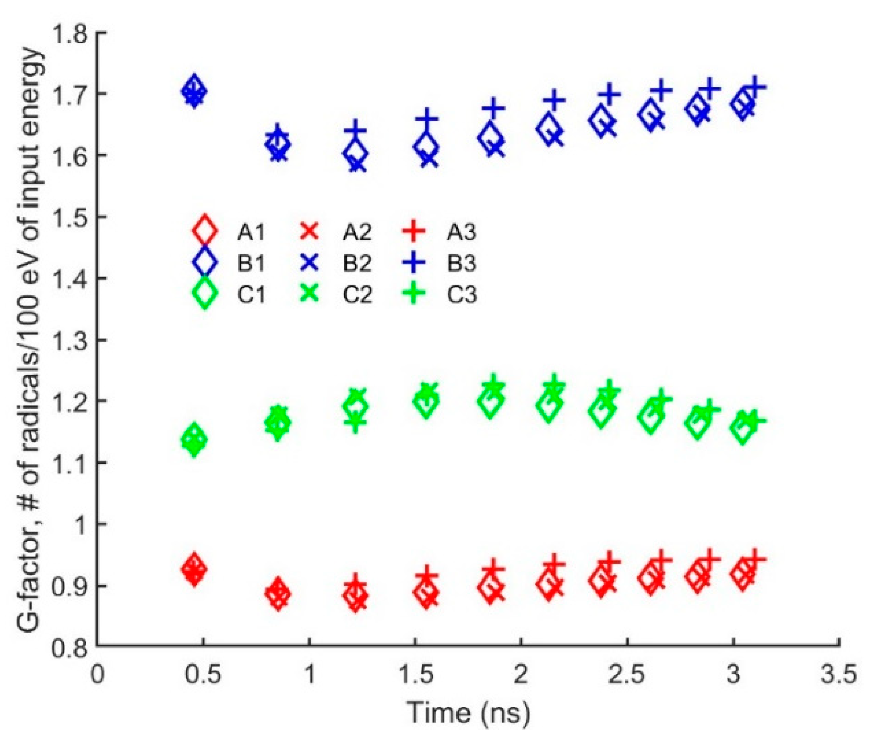
Figure 11.
The contribution of convective and gain/loss terms in the energy equation. The solid black line is the net rate of energy density change at the spatial position in axis. (a) the hybrid parametrization and (b) LMEA parametrization.
Figure 11.
The contribution of convective and gain/loss terms in the energy equation. The solid black line is the net rate of energy density change at the spatial position in axis. (a) the hybrid parametrization and (b) LMEA parametrization.
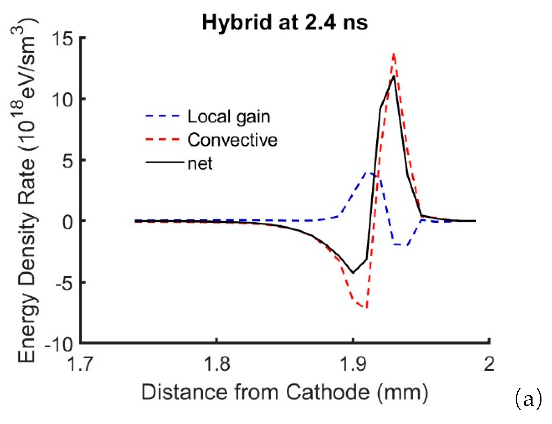
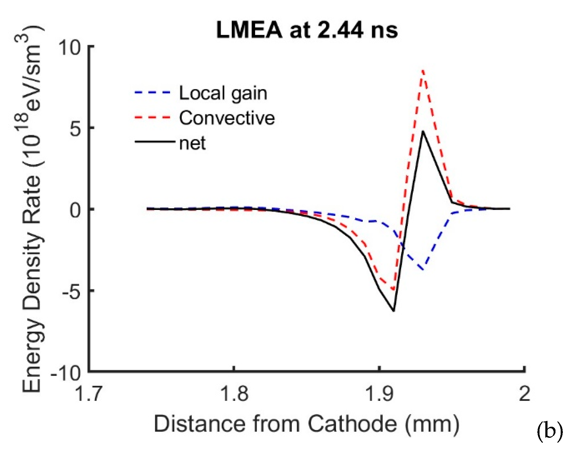

Table 1.
Parametrization schemes.
| Local-Field Approximation (LFA) | |||
|---|---|---|---|
| Local-Mean-Energy Approximation (LMEA) | , | ||
| Hybrid | , |
Disclaimer/Publisher’s Note: The statements, opinions and data contained in all publications are solely those of the individual author(s) and contributor(s) and not of MDPI and/or the editor(s). MDPI and/or the editor(s) disclaim responsibility for any injury to people or property resulting from any ideas, methods, instructions or products referred to in the content. |
© 2024 by the author. Licensee MDPI, Basel, Switzerland. This article is an open access article distributed under the terms and conditions of the Creative Commons Attribution (CC BY) license (https://creativecommons.org/licenses/by/4.0/).
Copyright: This open access article is published under a Creative Commons CC BY 4.0 license, which permit the free download, distribution, and reuse, provided that the author and preprint are cited in any reuse.


