
Submitted:
29 October 2024
Posted:
29 October 2024
You are already at the latest version
Abstract
In the context of the Bridge Electromagnetic Theory, a quantum-relativistic theory based on Maxwellian electromagnetism, it has recently been shown that the characteristics of a hydrogen atom can be obtained through an electron-proton orbital capture process forming a non-radial emitting dipolar electromagnetic source. The model structurally different to the Bohr-Sommerfeld and Schrödinger models has now been deepened and completed by testing it on the properties of hydrogen and deuterium atoms and of helium and lithium in hydrogenoid form. These last two atoms are of cosmological interest as they are the heaviest elements produced by electron capture in the early universe. The theoretical results obtained regarding the atomic structure and spectra are in excellent agreement with the observational data by suggesting the implicit correctness of the model. It is also highlighted that the electron-nucleus interaction is influenced on an isotopic basis as a function of the value of the inertial mass of the nuclei considered.
Keywords:
Non-standard Atomic Model
; Bridge Theory
; Electron Capture
; Energy Levels
; Spettroscopy
1. Introduction
Atomic ancient theory based on the Rutherford model
has changed over the years both conceptually and formally. In spectroscopy, the
current atomic model is fundamentally based on the Bohr-Sommerfeld theory [1], although the formulas for the determination of
spectral lines and energy levels use the Rydberg-Ritz principle [2] which allows the calculation of the wavelengths
of the emission spectra by means of ad hoc parameters identified on the basis
of the atomic element considered. From the point of view of Quantum Mechanics,
first the Schrödinger model, then the Dirac equation, were used to take into
account the dual wave-matter phenomenology of atomic electrons, thus providing
a probabilistic description of their momentum and position at each individual
atomic level.
In this work, we propose a new approach to atomic
model based on the Bridge electromagnetic theory (BT) principles, which has all
its foundations in Maxwellian electromagnetism [3–5].
In this model, quantum and relativistic phenomena, as well as wave-matter
dualism, emerge consistently from the theory used without forcing their
introduction, in fact, it is known that quantum mechanics and relativity work
well together even if their foundations are not compatible at all.
Bridge theory is a consistent and complete theory
originating from the conjecture proposed in Ref. [3]
on the role of the Transverse Component of the Poynting Vector (TCPV) of the
Dipolar Electromagnetic Source (DEMS) formed during the direct interaction
between two approaching charged particles of opposite sign (See also Ref. [4,5]). The TCPV is able to localize the amount of
energy and momentum inside the DEMS in the quantum form with a wavelength equal to the minimum distance of
interaction achieved by the two interacting particles and with the theoretical
value of the action constant characterizing the electromagnetic interaction of
the two particles. The extraordinary result obtained in the past is the value
of the action constant calculated using the theory is in agreement with
the standard value of Planck’s constant, thus demonstrating that quantization
is not a principle but a phenomenon that derives from the particular way of
interaction of a pair of charged particles.
The conjecture proposed in Ref. [3] on TCPV was subsequently proved in Ref. [4,5] by the calculation of Sommerfeld’s constant
and consequently by the determination of the physical origin of Planck’s
constant, subsequently allowing the development of an unconventional
electromagnetic quantum theory presented in Ref. [6].
Later it was shown in Ref. [7] that
relativistic phenomenology can also be explained using the same theoretical
approach. Therefore, despite appearances, Maxwellian electromagnetism, Quantum
Theory and Special Relativity are fully compatible theories and can therefore
be used together in the form of an electromagnetic quantum-relativistic theory,
the BT, whose formalism does not differ from that commonly used in QED, but
offers new insights into interpreting the physical phenomena observed.
2. The Bridge Electromagnetic Theory: Brief Introduction
In BT, the interactions that produce quantum
phenomena occur exclusively between pairs of charged particles of opposite
signs that are defined as pairs of charge and anticharge, as the quantum
behavior does not depend on the value of their original inertial mass, the
mechanical nature of which has been studied separately in Ref. [8].
The crucial point in BT is the formation of DEMS,
which bonds pairs of charges by producing an electromagnetic entanglement
independent of the distance achieved by the two particles. In fact, when DEMS
is formed, any change in energy and momentum on the particles that form it
would produce a change in energy in the DEMS which, however, for conservation
can no longer occur as it would violate the principle of causality. This
implies that a direct interaction in a pair of charges cannot be considered
completely Coulombian because two interacting charges are always in motion with
respect to each other, producing not only the Coulomb interaction but also an
electromagnetic interaction that generates a non-point perpetual dipole source,
i.e., the DEMS, which moving with respect to every other inertial observer,
produces with each of them a different Doppler effect that gives rise to the
relativistic phenomenology.
The electromagnetic field of the DEMS does not
have, therefore, spherical symmetry as the Coulombian one but cylindrical
symmetry with the symmetry axis coinciding with the dipole moment axis, so the
Poynting vector is not everywhere radial and the emerging wave can be
considered a composition of a spherical radial wave that describes the
classical field with a plane transverse wave circulating around the virtual
center of the DEMS that originates quantum effects. Each observer external to
the direct interaction receives a superposition of both waves characterized by
a Doppler [7] the value of which defines the
observed energy and momentum in full accordance with Special Relativity.
In the following sub-chapters, the fundamental
conceptual and theoretical elements of the theory necessary for the
construction of the atomic model will be resumed.
2.1. Quantum Behavior: Poynting Vector, Action and Energy of a DEMS
The electric field of the dipole can be described
by a local three-dimensional vector centered in the dipole having at each point
of the spacetime three unitary components : lateral, transverse, and radial, of which the
lateral component is always zero (Cf. Ref. [5,6]).
In Gaussian units, the electric field of the dipole
is:
(1)
whose only two non-null components are functions of
the parameters . The first is the most important and is defined by
the ratio , where is the variable distance between the two
interacting charges, corresponding to the length of the dipole moment for the
unit of charge and the wavelength of the electromagnetic wave that will be
emitted by the DEMS produced. The second is the polar angle between the radial
vector pointing to a point of spacetime and the dipole axis, whereas the
magnetic field of the DEMS in the dipole wave zone is
(2)
consequently, the Poynting vector of the
electromagnetic field
(3)
is characterized by a nonzero transverse component that localizes within the wavefront of the DEMS,
an amount of energy and momentum, and by a classical radial component associated with the spherical radial wave.
For each interaction occurring between a pair of
particles, the physical conditions change. Therefore, the value of the
parameter must be recalculated using a stochastic process
defined by the constraints produced by the external forces acting on the DEMS.
In the case of free interaction, when a pair of particles interacts without
external constraints, the value of the ratio was statistically accurately estimated (Cf. Ref. [5,6]), and the best value obtained is . In this case, with reference to Eq. (3), let , the energy of the localized quantum is calculated
by the expression
(4)
where is the theoretical value of Planck’s constant for
free interactions described in Dirac form. Eq. (4) describes the energy and
momentum exchanged in the form of a photon by two interacting charges.
The energy, as shown in the second row of equation
(4), is described by two dimensionless contributions, one electrostatic (es)
and one electromagnetic (em), which define and estimate the value of the
total structure constant as a function of the mean value characterizing the DEMS.
Because the value of the structural constant during
a free interaction is equal to the reciprocal value of Sommerfeld’s constant,
the coupling constant can be considered a universal constant with which
it is possible to define the value of Planck’s constant.
For
what has been written above, in BT the values of , , are not true constants because they can vary, even
if only slightly, as a function of the boundary conditions that define the
physical reality in which the DEMS is formed, i.e., as a function of the forces
acting on the interacting charges. In fact, for free interactions, Sommerfeld
theoretical constant is in very good agreement with the one calculated
experimentally, except for a very small difference due, in the case of theoretical
calculation, to the lack of direct interaction of the DEMS with the observer.
In other cases, the boundary conditions can significantly modify the value of and, consequently, the values of the coupling
constant and action unit.
Considering an electron-proton interactions, the
energy and momentum that characterize the DEMS are the energy and momentum
associated with the initial reciprocal free motion of the particles before
electron-proton capture takes place and represent the energy and momentum
exchanged in the interaction in a limited time interval. In fact, contrary to
what occurs in the strictly Coulombic interaction, the interaction associated
with a DEMS has a finite duration and occupies a finite space (Cf. Ref. [6]).
During the electromagnetic interaction of a pair
of particles, the start of the interaction corresponds to the zero-energy
emission from the source, which is associated with an initial zero value of the
radial Poynting vector. In agreement with BT, the value of the radial component
of the Poynting vector increases over time by increasing the brightness of the
source as the distance of the wavefront from the virtual center of the DEMS
increases, reaching the maximum emission after a characteristic time equal to half of the total interaction time; then,
the energy emission starts to decrease when the particles reach the minimum
interaction distance, which is equal to the wavelength of the source, and
begins to move away, increasing their interaction distance. Under these
conditions, an electron and a proton forming a DEMS exchange a photon of energy
and momentum (4) equal to that which the DEMS will gradually emit by means of
the radial component of the Poynting vector; therefore, the DEMS cannot be a
stable system.
As previously described, the Sommerfeld constant in
the context of BT is calculated from the characteristics of the electromagnetic
field structure of the DEMS in spacetime. Its value in the case of free
interaction between pairs of particles or particles of different masses but
with charge and anticharge corresponds to , whose value is in agreement with the most recent
value measured experimentally in Ref. [9].
The most recent theoretical value of Sommerfeld’s
constant was calculated in the context of BT and is presented in Ref. [10] because of the formation of a hydrogen atom
during the electron-proton capture process. The estimate obtained with the
formation of the hydrogen atom gives an extremely precise and stable value of
the coupling constant , which differs from that obtained in the case of
the free interaction of ppm and from that obtained experimentally from ppm (cf. Ref. [9]).
The difference between the theoretical and experimental values was due to
different physical contexts. In fact, the theoretical value of the
fine-structure constant is obtained in the interaction process without the
system interacting with external observers, and thus, is altered.
2.2. Relativistic Behavior: Energy and Momentum of a DEMS
Because the observation of a DEMS involves the
measurement of the energy and momentum of each its component, in the simple
case of a hydrogen atom formed by an electron and a proton, both are perceived
by an external observer as two moving particles, each with its own energy and
momentum, and with velocities referred to the Lab.
As proven in Ref. [7],
an observer placed on one of the two particles in interaction feels the other
as carrying all the energy and momentum that will form the DEMS. This has
already been applied in Ref. [10] to simulate
hydrogen formation with electron-proton capture, therefore, the total energy
and momentum of hydrogen in formation correspond in according with the BT to
those of a material particle with energy and momentum equal to those of the
relativistic approaching particle:
(5)
From the point of view of the proton, is the resting mass energy of the electron in
motion, and are the Lorentz factor and the velocity of the
electron divided by the light speed at the time of the interaction, respectively.
2.3. An Atom Described by a DEMS with Zero Radial Emission
In general, when a DEMS is formed it emits a wave
which propagate in all direction energy and momentum. To obtain the conditions
under which the DEMS has null radial emission becoming a stable atomic system,
it is necessary to examine the emissive conditions of the dipole.
Let us begin considering the local electromagnetic
contribution to the radiated energy for a DEMS in a given direction (Cf. Ref. [6])
(6)
Equation (6) can be usefully analyzed by
introducing the local brightness vector , defined as:
(7)
so that Eq. (6) can be rewritten as
. (8)
with infinitesimal element of the surface of the ideal
sphere, through which the luminosity is flowing.
By setting , where and describe the radial and angular behavior of the
Poynting vector, respectively. To have a physically correct behavior for the
emission of energy from the source with arbitrary value of electric charge, it is
necessary that
. (9)
The length of the Poynting vector in Eq. (7), which
transports the energy of the source, coincides with the radial component of the
Poynting vector of the dipole.
(10)
where denotes the angular distribution of the radial
part of the Poynting vector.
To analyze the radial emissions of a DEMS, Eq. (7)
can be written in polar coordinates as follows:
. (11)
By setting the depth of field variable and neglecting the angular behavior, we define
. (12)
and equation (11) can be rewritten as
(13)
the general solution of which
(14)
describes the behavior of the local brightness on
the surface of the spherical shell as a function of .
For fixed wave number and for , the wave converges to that emitted by an ideal
point source; therefore, considering the asymptotic behavior of Eq. (14), we
obtain the luminosity on the surface as
. (15)
Comparing
equation (14) and (15), we can see that a DEMS emits less energy than a point
source, and the difference in brightness is
. (16)
This implies that an amount of energy proportional
to Eq. (16) was retained within the surface and was located in the volume around the DEMS. As
the emission of energy from the source is continuous, there is a characteristic
equilibrium spherical surface for which the energy emitted through the surface
is equal to that not yet emitted. Because the wavelength characterizes the
period of the wave, it is assumed that equilibrium is reached on the first
wavefront of the DEMS for . Using equations (15) and (16), we can then write
the equilibrium condition as
, (17)
whose solution gives . Consequently, the brightness turns out to be
(18)
that it is equal to zero in for each angular direction by reaching the maximum
brightness for . The extremes of the interval delimits the spherical crown defining the source
zone (SZ) of the DEMS, so for the radial emission of the DEMS is not active, and
the DEMS absorbs energy and momentum from the impinging interacting particles and for the production of energy of the DEMS is ended.
Considering
an atom formed by the mutual electron-nucleus capture of charges , both associated with an inertial mass with a
proper value of energy at rest, the total input energy described by Eq. (5) can
be used to power the rotational energy of the system around the center of mass
of the source (Cf. Ref. [10]). When capture
occurs and the electron orbits around the nucleus at a fixed orbital distance , the round bracket in Eq. (18) becomes null
(19)
therefore, the dipole cannot emit radially and the
brightness (18) becomes zero. In this case the electron and nucleus form a
bound state in which the wave propagation occurs only with the transverse
component of the Poynting vector along a circular path inside the spherical
surface delimiting the internal border of the SZ of radius
.
Remembering that the electron-nucleus interaction
localizes fundamental energy and momentum with , by generalizing the interaction energy at a
multiple of the fundamental energy as with , using the radial field depth variable , Eq. (14) becomes
. (20)
that cancels for . Therefore, the spherical shell bounding the virtual center of the source is a
surface with zero radial emission. A captured electron in motion on this
surface maintains a constant distance from the nucleus, so that the DEMS does not emit
radially. It follows that the surface represents a sphere on which the radial component
of the Poynting vector is everywhere zero and the transversal one propagates
the electron as a local stationary wave of energy . From the perspective of the nucleus, which has a
higher mass than the electron, the captured electron forms a circular path
centered on the nucleus with a radius . Under these conditions, the complete DEMS rotates
around the nucleus taken as like a fixed point describing an electromagnetic
field within a toroidal spacetime of extreme radius by defining the outer radius of the stable atom
with energy equal to that of the n-th energy level with effective
orbital radius .
In the ground state, the DEMS will emit radially
only when the electron is stimulated by external fields to change the energy.
In fact, during the transition between two different energy levels, a non-zero
radial component of the Poynting vector is produced. After the emission of the
excess of energy, the atom becomes stable again, returning to the ground state;
if the system is destabilized by the transfer of more energy than that which
characterizes the electron bond, the atom ionizes, returning the captured
electron to the environment.
2.4. The Concepts of Electron Spin and Atomic Spin in BT for Two Fermions
In quantum mechanics, spin is a fundamental
characteristic of the particles. It is considered a form of angular momentum
that is intrinsic to particles and is independent of their motion or position. This phenomenon of quantum mechanics has no equivalent in
classical physics.
Following BT, the spin is explained considering
that each particle of charge is entangled with all the anti-charges with which they are causally connected forming
independent DEMS independently by their distance of interaction (Cf. Ref. [6,7]). For an atom of hydrogen, using the field
vector defined in equation (3), the angular momenta
associated with the hemispheric zones of a DEMS containing the positive or the
negative interacting charges (IC) forming the DEMS, in units of , are defined as the field spin down and up of the
IC:
(21)
where is the transverse component of the vector and is the same component for switched charges (Cf.
Ref. [6]). Thus, the sign of the spin of the
particles depends on the frame in which the interaction is observed.
Extending the calculation to the complete SZ and
assuming the dipole axis as the axis of symmetry, by integrating the angular
functions over all directions, we obtain a null total spin for both unswitched
and switched charges:
. (22)
In this case, the frame invariance provides the
null spin values of the source as a unique effective component.
Considering the electromagnetic emission of the
source, the directions of propagation of the photons are along the wave number direction, which is normal to the dipole axis.
Then, for an observer, the angular momentum can be naturally calculated using
the propagation axis as the axis of symmetry around which the dipole moment
spins during the interaction. By calling the angle measured around this axis, we obtain:
(23)
The
two components of this vector are the spin components corresponding to the left
and right circular polarizations of the wave, that is, of the emitted photons;
however, in this case, an atom does not emit; therefore, the spin component
(23) for an atom of hydrogen in stable conditions may not be considered.
Therefore, for an atom of hydrogen there are DEMS components and it is possible to define three
types of spins: atomic spin (22) for atoms in the fundamental state which is
unobservable; electron spin (21) for the two particles forming the DEMS; and
emission spin (23) for non-stable atoms. This spin value defines the
orientation of the emission axis of DEMS. It is important to emphasize that the
spin of a single particle continues to exist even when the particles have
reached a great distance because the DEMS continue to exist also if the amount
of localized energy is near to zero; therefore, spin is a property of the
particle and indicates the existence of an interconnection with other
particles. In this sense, the DEMS group all electromagnetically connected
particles into pairs, creating a type of electromagnetic entanglement (Cf. Ref.
[7]).
In summary, two interacting particles in pair can
have spin , whereas the DEMS formed using and can have spin , where the null value always refers to the
unobservable ground state of the hydrogen.
3. The Atomic Model: Kinetic Energy of the Orbiting System after Electronic Capture
In compliance with one of the fundamental
principles of BT (Ref. [6]), the capture of
one electron by the nucleus during the atom formation takes place in the form
of a charge-anticharge interaction, forming a number Z of independent
DEMS.
For simplification, we consider the atom of
hydrogen in formation as an isolated system electron-proton, with the
transverse component of the momentum of the electromagnetic field associated
with the TCPV of the DEMS
, (24)
from a mechanical point of view, the electron in
motion along its trajectory has respect the proton total momentum with angular momentum
(25)
Before capture when the electron is at a great
distance from the proton , therefore , for the conservation principle the time
derivative of Eq. (25) must be equal zero maintaining constant the original
null angular momentum
(26)
that implies that even after the formation of the
atom, in the ground state the angular momentum (25) must be zero. In fact, the
spin of a DEMS in Eq. (22) returns as a value .
As shown in Ref. [4,6],
for a DEMS, the two addends in Eq. (26) can be interpreted as the sum of two
opposite energies. The first is the expansion energy of the SZ due to the
radial propagation of the electromagnetic field of the DEMS, while the second is the rotational energy associated with the spin
of the field due to the circular propagation of the transverse component of the
Poynting vector around the center of the DEMS.
From a mechanical point of view, during DEMS
formation, is provided by a force acting radially on the
electron-proton system. In fact, the strength of the radial force being less than zero is attractive in such a way
that energy is positive. Considering the DEMS point of view,
the velocity of propagation of the electromagnetic field along the radial
direction is . From Eq. (26) and from the definition of the
force acting on the moving electron, we can write
. (27)
During the capture process, the Coulombian
interaction is always active; instead, the electromagnetic interaction mediated
by the DEMS connecting the two particles is active only during a short period
of time defined from the instant at which the source zone (SZ) of the DEMS
starts at a reciprocal distance until the SZ stops producing energy at the
reciprocal minimum distance of interaction . Therefore, the total mechanical momentum acquired
by the system at the end of the capture process is given by:
(28)
that correspond to the conservation of the total
transverse component of the momentum acquired by the electromagnetic field of
the DEMS, therefore using Eq. (27) and (24), the total momentum (28) associated
with the field spin is obtained by integration in the form
(29)
In general, considering the Coulombian force active
between electron and nucleus,
(30)
in SI units Eq. (28) yields the total field spin
energy acquired by the system:
, (31)
when the electron and nucleus reach a minimum
interaction distance corresponding to the de Broglie wavelength of the electron (Cf. Ref. [7,10]), the energy
(32)
of the quantum exchanged between the electron and
the nucleus acquired by DEMS, propagates by the TCPV on the internal surface of
the SZ of the DEMS keeping the energy of the atom stable.
In Eq. (32) is used as the standard symbol of the
Planck action in Dirac form , because in this case, the photon refers to a free
interaction between charge pairs where the value of the action constant
corresponds to Planck’s one, and in the case of the use of the Sommerfeld
fine-structure constant the symbol is , when necessary, the symbol for the different
orbit levels will be diversified to avoid confusion.
Because the total energy (32) exchanged during the
interaction cannot involve photons with energies greater than that which
characterize the DEMS of a single electron-proton interaction given in Eq.
(32), the total energy exchanged in the process of electron capture can only be
a multiple of this fundamental energy:
(33)
Since the center of mass of the atom refers to an
observer placed in the laboratory system, using Eq. (31), (32), and (33), in
accordance with the four-momentum invariant (Cf. Ref. [10]), the total mass energy at rest calculated in
the center of mass of the system is given by
. (34)
Substituting in Eq. (34) and the respective
equations (31), (32), and (33), the rest energy of the atom gives
(35)
with beta ratio of the electron
(36)
and orbital Lorentz factor, . From Eq. (31), (35), and (36), the capture energy
(33) of the electron can be written as the identity
, (37)
where
the minimum interaction distance is the de Broglie wavelength of the electron in
the n-th energy level, that is, from the relativistic point of view, gives
(38)
with fundamental pseudo-orbit wavelength calculated
as
. (39)
It is convenient to observe now that Eq. (39) gives
as the natural limit of the atomic number for the formation of a stable atom . The existence of this limit in agreement with
Chandrasekhar prediction [12] that normally
has to do with the nucleus stability let us to suppose that the formation of
the atom is more related of haw one can think to the nucleus formation.
The calculus of the orbital radius for the n-th
energy level defined by the Eq. (37), is given by the condition of coherence of
the electromagnetic circulating wave, i.e., the effective length of the
circumference of the orbit on which the wave propagates stably must be equal to
a multiple of the de Broglie wavelength of the atomic system, because the electron
cannot have a de Broglie wavelength different to the capture one defined by the
Eq. (32): . By Eq. (38), we obtain the radius of the
pseudo-orbit which characterizes the n-th quantum state of the atom
(40)
The pseudo-orbit is a circle of radius (40) on
which the electron is described by a circulating electromagnetic wave. For
atoms with Eq. (40) can be approximated in the form with Bohr radius of the hydrogen.
Because the energy localized by the capture was
completely transmitted to the system, Eq. (37) can be rewritten using the
reduced mass energy at rest of the electron-nucleus system rather than that of
the electron, that is, one replaces at the reduced mass energy
, (41)
therefore,
following the founding principles of BT, to calculate the kinetic energy of the
orbiting system is enough to subtract to the capture energy (37) relative to
the orbiting system its energy at rest (41), therefore, in accordance with
Special Relativity for the kinetic energy one obtains
. (42)
It is very important to consider than each electron
captured by a nucleus on the n-th pseudo-orbit must have a different
fine structure constant defined by the constraints condition on which is
subject, therefore, for each energetic level one will consider the
characteristic fine structure constant which is only a bit different from the value
defined for a free interaction.
4. Effective Energy at Rest of a Nucleus
In Eq. (41), it is necessary to estimate the value
at rest of the mass energy of the nucleus; therefore, for a fixed atomic
number with a number of neutrons, one can define the isotopic number. Considering that only the
DEMS formed by electron-proton interactions contribute to the total energy of
the atom, the presence of neutrons in the nucleus partially shields the
positive charge by affecting the amount of energy available for the
interaction. In fact, for a fixed value of , when the number of neutrons increase, neutrons
and protons are arranged in such a way to maximize the stability of the
nucleus. Therefore, the energy of the resting mass of the nucleus participating
in the formation of the DEMS during the interaction with the orbital electrons
cannot be higher than that of the protons forming the nucleus, therefore, it
can be assumed that the mass of the nucleus participating in the reduced mass
of the system is a fraction is lower than that of the nucleus and can be supposed
to be proportional to the nucleus mass by a fraction
(43)
of the effective mass energy of the nucleus.
Considering an element with its isotopes family, each with relative
atomic mass with , and abundance , the average atomic mass of the mixing of the
isotopes of the element gives
(44)
which is equal to the sum of the atomic number , of the mean number of neutrons weighted as a
function of their isotope abundance
, (45)
of the atomic electrons expressed in amu
(46)
and of the excess or defect of mass characteristic of the considered nucleus, i.e.,
. (47)
Considering that for an element , the resting mass energy associated with the
effective nucleus, that is, the fraction of the average nuclear mass
electrically active of a natural isotopic mix of the same element can be
defined by considering the charge fraction (43) of the effective mass energy:
(48)
by using the fraction (43) with the effective mass
(48) one obtains
. (49)
For
an isotopic mix of the element , Eq. (49) becomes
. (50)
Considering the natural mix of atoms formed by the
fundamental isotopes of hydrogen and , is neglectable, the resting mass energy (50) gives
instead of pure and . In both cases, the evaluations are lower than
that of the remaining energy of the proton because of the use of the energy of
an atomic mass unit: estimated for an atom of , but in the case of the natural mix of hydrogen,
the value is even lower because of the shielding effect due to the presence of
neutrons in the nucleus of deuterium. In all cases, the differences in the
model results were minimal, and Eq. (50) is suitable for hydrogen and deuterium
atoms, and can be extended to more heavy atoms as helium and lithium.
5. Quantum Numbers
Eq.
(33) is the energy acquired by the atomic system once after electron capture,
stability is achieved. This value includes the mass energy at rest of the
electron and the rotational kinetic energy provided during electron capture.
The integer value can be thought to consist of two components: a
number that defines the multiplicity of the action
associated with the radial momentum and a number that defines the multiplicity of the action
associated with the angular momentum supplied to the nucleus during the
electron capture in such a way that with degenerate energy states associated with all
their combinations without the orbit to be elliptical, as predicted by the
Sommerfeld model, because this shape would produce a radial emission in the DEMS. To
simplify, in accordance with the Bohr-Sommerfeld model, the principal quantum
number and secondary quantum number in such a way that .
Because the spin of an atom in the fundamental
state is always zero because the two particles forming each single DEMS have
opposite spins, for excited atoms subject to external fields, the spatial
orientation of the photon emission can be defined by a new number obtained as
the product with values . This number is consistent with the role of the
magnetic quantum number, and is in fact different from zero only if the atom is
plunged in an external electromagnetic field, assuming a precise orientation up
or down with rotational kinetic energy defined by the secondary quantum number.
Therefore, it is possible to define the complete state of the electron and its
atomic system using the spin of the electron and the set of quantum numbers defining the state of the atomic system in the
environment.
6. The Wave Behavior of an Interacting Electron: Orbital Eigenvalues
As discussed in Ref. [11]
and in the estimation of the Sommerfeld constant during the formation of a
hydrogen atom by the electron-proton capture (Cf. Ref. [10]), an electron during its interaction with a
positive charge as a nucleus gives up all of its energy at the DEMS, and its
propagation is described by a wave described by the linear differential
equation:
(51a)
with solutions:
(51b)
The first part of Eq. (51b), defined as the wave
function it is associated with the corpuscular
characteristics of the captured electron, which carries the residual momentum
of the electron corresponding to the momentum not yet transferred in time in
other interactions, that is, the residual momentum , whose value is always less than or equal to the
Galilean momentum of the electron (Cf. Ref. [8]), and represents the total momentum transferred
to the system during the capture process at time . The second part of Eq. (51b) is a wave function describing the system before and after the
interaction by carrying information regarding the energy and momentum of the
moving electron.
For
an atom, the interaction between electron and nucleus is stable and is
described over time as a DEMS formed in the time interval with action . In this case, we can consider the system electron
nucleus, as described by the full wave function part of Eq. (51b), which describes the momentum
exchange. In this case, the wave equation (51a) can be rewritten in the reduced
form as , with , which can be considered the Hamiltonian operator
of the stable system, variable only on time, with eigenvalues of the energy exchanged, corresponding
to that after electron capture with becomes the capture energy (33), that is, .
7. Electron Bond and Orbital Energy
The captured electron rotates with the nucleus around the common center of mass with a rotational kinetic energy equal to Eq. (42), which balances the attractive force, such that the sum of the orbital relativistic kinetic energy with the binding energy is zero: . This condition implies that the energy that characterizes the capture of electrons in the n-th orbit of the ion must be opposed to the relativistic kinetic energy of the electron, using Eq. (42) and using the values of the modified fine structure constants expressed as a function of the first quantum number associated with the n-th capture level, computed using the recursive correction method examined in Ref. [10] and revised for atoms with Z protons in Appendix A, the binding energy of the n-th orbit is given by
. (52)
with .
8. Atomic Energy Levels
To define the energy levels of the DEMS model of an atom, it is necessary to consider the difference in the binding energy (52) between the fundamental level with and another level , which is equivalent to the difference between the capture energy for an electron bound to the bare atomic nucleus and the capture energy at a level other than the principal quantum number. Using Eq. (52), we can write:
. (53)
with , standard value of the Planck constant obtained for an electron-proton free interaction during the transition between levels.
8.1. Hydrogen and Deuterium
The estimations of the energy levels for hydrogen in Table 4 and deuterium in Table 5 are presented. Using equations (41), (52), and (53) and the orbital fine structure constant shown in Table 1, the fundamental level of hydrogen, corresponding to the quantum number , has a binding energy equivalent to . This value is only slightly lower than the Rydberg energy of the atom; thus, of the kinetic energy of the electron measured immediately before the capture process begins (see Ref. [10]). In fact, both values are greater than because the effective resting energy of nucleus is defined by Eq. (49) with being only slightly lower than the energy of proton ; therefore , Eq. (41) gives a reduced mass energy of the system only after the electron capture occurs, whereas before electron capture, the kinetic energy is that of the impinging electron, and the mass energy involved is independent of the mass of the proton because of the delay in the propagation of the electromagnetic field during the DEMS production. The proton can be considered not involved, that is, the proton is perceived as having an infinite mass by giving . In this case, the relativistic kinetic energy of the electron was greater than that of . In addition, in the case of Rydberg energy, the experimental value is measured during the process of ionization of the atom, that is, during a non-relativistic ejection of the electron in which the total energy is that of the resting mass energy.
The calculation for deuterium is similar to that performed for hydrogen, considering the effective resting energy of the deuterium nucleus defined by Eq. (49) using one obtains . In this case, the fundamental energy level for deuterium (D) calculated using Eq. (52) is given by , with energy lower than that of hydrogen.
8.2. Helium and Lithium
To extend the model to atoms with , it is interesting to consider helium with and lithium with . These two atoms are interesting because they are the heaviest elements produced during non-stellar primordial nucleus-synthesis. The procedure for calculating the energy levels was the same as that for hydrogen. The energy levels for helium and lithium are listed in Table 6 and Table 7, respectively.
9. Spectral Lines
To calculate the emission spectrum wavelengths for excited atoms, it is necessary to consider the change in energy of an atom or ion when the electron-nucleus system receives sufficient energy to change the energy state of one or more DEMS. If the energy received is sufficient to change the state of the system, the electron moves on the spherical shell, which corresponds to the energy absorbed at a wavelength con at a distance from the nucleus, and then after a time returns to the original orbital emitting the surplus energy by means of a photon. Using the binding energy (52), since the excited final state has a lower binding energy than the initial ground state , with , for the return energy jump the use of the first part of Eq. (37) yields the emission wavelength:
(54)
with
(55)
and , Lorentz gamma factors are associated with the initial and final energy levels between which electron transitions occur.
From a phenomenological point of view, atoms emit only when they acquire enough energy to modify the pseudo-orbital of one or more electrons by transforming into emitting DEMS This process, called atomic excitation, consists of distributing an arbitrary amount of energy to the electrons of the atom starting from the outermost electrons that have a distance of interaction with the nucleus and an energy of greater bonding than the innermost electrons. In this way, in a power process, in which all the electrons of the atom acquire sufficient energy over time to move to higher energy levels, the atom behaves as a multi-dipole source (DEMS) by emitting chromatic photons associated with the excess energy acquired by the electron-nucleus system. The consequent effect is the return of the electrons to their original configuration. The process described involves each electron undergoing slippage during the level jump that involves the exit from the condition of atomic stability, inducing the transformation of the atom into a multi-dipole source with consequent chromatic emission of energy forming the characteristic spectrum. The orbital slippage causes the electron to move for a limited time on a noncircular trajectory, not necessarily elliptical, with respect to which the fine-structure constant differs from the exact value of the corresponding layer; therefore, a correction that takes into account the shift is necessary. Table 7 shows the correction ratios obtained empirically, considering the positive and negative orbital slippage of electrons during jumps between the energy levels. The corrections proposed are obtained by modifying the value of the fine structure constant of the outer layer such that the emitted spectral line corresponds to the experimental observation, which corresponds to a model that agrees exactly with the measured emission spectrum. In Table 8, Table 9 and Table 10 are tabulated the estimations of the principal transition lines of the Lyman, Balmer, and Paschen series for hydrogen and Table 11, Table 12 and Table 13 for deuterium. The correct values for the orbital slip are displayed in the third column.
(56)
10. The Bohr Model as First Order Approximation of the DEMS Atomic Model
Considering McLaurin’s development of the orbital gamma factor in Eq. (37)
(57)
Eq. (52) makes
(58)
using Eq. (58), the difference in capture energy in the two levels given bycan be considered to be formed by a change in rotational energy and a change in the vibrational energy of the atom plus other terms that are negligible because they are not experimentally significant.
(59)
whereas the vibrational term is less than times the rotational term, and because the shell-to-shell electron jumps change the rotational energy of the system, but not significantly the zitterbewegung of the nucleus, to simplify Eq. (59) It is possible to assess the intensity of the energy transition spectral line by considering only the contribution to the rotational energy change in Eq. (59). Thus, using equations (59), (52), and (55), the reciprocal of the wavelength of the photon emitted by the atom during a transition is given by
(60)
To simplify, considering that for orbits the values of the coupling constants are , their value is replaced by that of the free value of the fine-structure constant . Eq. (60) becomes
(61)
Equation (61) describes the emission line in the transition associated with the electron-nucleus system, and can be rewritten in the classical spectroscopic form:
(62)
where using Eq. (55) in (61), Rydberg’s constant in Eq. (62) in SI units is given by:
(63)
that for an atom of hydrogen, the value of the constant (63) with is ; therefore, Eq. (63) can be rewritten as in agreement with classical spectroscopy.
This paragraph aims to prove that the DEMS atomic model is consistent in the first approximation to the Bohr model.
11. Effective Nuclear Mass
According to the Bridge theory (Cf. Ref. [8]), any electromagnetic interaction between electric charges in motion generates an inertial mass. By contrast, each inertial mass corresponds to an electromagnetic interaction that produces it.
The existence of a pair of interacting charges (e.g., electron-proton) leads to the creation of a DEMS of limited space-time extension that moves following a trajectory linked to the dynamic characteristics of the interacting particles. The overall energy and momentum of the DEMS correspond to the total energy and momentum of the observed system, in which the resting masses of a particles pre-exist the DEMS and represent the energy retained at the time of their formation starting from one or more events that generated them through a decay or assembly of other particles. At the present stage of BT development, it can be assumed that the phenomena that initiated the resting mass energies of particles are associated with the formation of space-time, but this topic is unrelated to this work.
During the direct interaction of the particles, all available energy is converted into electromagnetic energy of the DEMS, but only during the life of the source. In the case of a DEMS at zero-emission, i.e., an atom, the duration is indefinite, therefore, the total electromagnetic energy of the atom must correspond to the total inertial mass of the observed system. In particular, considering an atom from the point of view of the electron, the sum of all quantum jumps between the possible energy states must correspond to the available energy equivalent to the rest mass energy of the atom.
Let’s check it out. The energy relative to each possible orbit is considered. We define multiplicity as the number of times the reduced mass energy of the electron-nucleus system, very close in value to the resting energy of the orbiting electron, is contained in the resting energy of the atom
(64)
Equation (64) is equal to the maximum number of possible electron-nucleus orbital interactions, based on the available energy associated with the total resting mass of the nucleus. Using Eq. (37) Each energy level corresponds to the capture of electrons whose energy is equivalent to a fraction of the total mass energy of the dipole system:
(65)
Using the total capture energy (65) and summing the possible quantum levels determined by the ratio (64), the total energy
(66)
that can be engaged during all possible nucleus-electron interactions cannot exceed the total resting mass energy of the nucleus-electron system. The gamma factor in the McLaurin series was developed. The Eq. (66) gives
(67)
In the case of a hydrogen atom with , Eq. (65) provides the rest mass energy of the atom , showing that a fraction of its total mass energy is shared electromagnetically through the quantum levels that are formed during the interaction between the nucleus and the electron. In other words, the proton interacting with the electrons grants each quantum level a portion of its mass energy [13]. Consequently, generalizing, the sum of all capture energies associated with the quantum levels of an atom, is the effective rest mass energy of the nucleus-electrons system.
12. Discussion
In this work it has been proven that the atomic model based on the Bridge Theory is able to provide a perfect description of the atomic phenomenology, with the advantage, compared to the Bohr-Sommerfeld-Schrödinger models, of introducing quantum principles and Special Relativity in a way self-consistent with the Maxwellian electromagnetic theory, as both quantum and relativistic phenomenologies derive from the particular way of interacting in pairs of moving charged particles. This approach is completely theoretical without require the use of experimental or measured data and in this sense, it could be asserted that the consistency of the results obtained cannot be considered a coincidence at all. The adequate use of the principles of BT could therefore lead to a formal and phenomenological revision of QED in which the typical concepts of quantum indeterminism and wave-particle dualism disappear in favor of the principle of electromagnetic interaction in dipoles, which from a phenomenological point of view allows to replace the concept of Coulombian interaction with that of direct electromagnetic interaction, which transforms through DEMS all the energy of the interacting system into electromagnetic energy localized in the form of exchange photons and the atoms into DEMS with zero radial emission, simplifying the phenomenology of the elementary electromagnetic interactions of matter.
Considering the atoms examined, the good agreement shown by the calculation of the radii and energies of the atomic levels and of the spectral lines of the atoms H, D, He, Li, suggests how the orbital capture may be the only way to produce a large amount of monatomic hydrogen in a cooling universe in which electrons and protons can have been produced in perfect symmetry.
Although the model shows that the orbital motion of atomic electrons around the nucleus is relativistic, from a spectrometric point of view, the first-order approximation of the model leads back to Bohr’s model, thus demonstrating its substantial correctness in terms of first principles.
13. Conclusion
The theoretical results of the spectra obtained were presented both in the exact form and in the modified form. The modify form is necessary to match the theoretical data with the observational one and it is produced by the corrections introduced based on the principle of the orbital slippage of electrons due to the absorption of an excess of external energy, which produces the continuous passage of an electron from the fundamental orbit to a more energetic one. The proposed correction, although currently is obtained in a semi-empirical way, is based on the principle that the fine-structure constant varies as a function of the orbit because the dipole moment of the electron-nucleus system changes in continuous for each orbital motion.
Finally, it is shown that the electron-nucleus interaction changes on the basis of the nuclear isotopy due to the different inertia of the atomic nucleus and that only the mass energy of the charged fraction of the atomic nucleus can contribute to the binding energy of the system. Therefore, the sum of the energies of all the orbital levels of the atom is equal to the mass energy of the active atomic nucleus and its captured electrons.
The atomic model developed in the present work is completely obtained using the Bridge Electromagnetic Theory (BT), that means that not has required the introduction of external physical concepts, in fact, quantum and relativistic formalisms appearing in the model are completely consistent with BT because developed inside the theory in Ref. [1,2]. In this sense, the atomic model is obtained using only the Maxwell’s electromagnetic theory, further expanded by the introduction of the typical concepts of BT.
Funding Statement
This study is not supported by grant.
Ethical Compliance
In these studies, no procedures involved human participants.
Data Availability Statement
No data associated in the manuscript.
Conflict of Interest declaration
The authors declare that they have NO affiliations with or involvement in any organization or entity with any financial interest in the subject matter or materials discussed in this manuscript.
Appendix A. The Calculus of the Orbital Sommerfeld Constant
Let us consider an observer placed on a point P of an ideal expanding spherical surface inside which a dipole with fixed polarization in space and dipole moment is placed. The energy per unit time pertaining to an infinitesimal portion of the expanding surface is equal to the flux of the Poynting vector of the source through the infinitesimal surface . The total energy observed in P during the time interval is given by:
(A.1)
where the radial component of the Poynting vector in Eq. (3) is parallel to direction of the surface element.
Such an observer sees the emission of the source just along the direction characterised by the angles , but by isotropy it assumes that the source emits in all other directions as it does in the direction in which it observes the source, i.e., that the DEMS has a spherical symmetry as in a point-like dipole where are identical and rewrites the Eq. (A.1) as
(A.2)
By Eq. (A.2), the total energy observed in P during the time interval is
(A.3)
where is the energy density contribute inside the spherical crown of volume associated with the energy emitted along the direction of P in the time . Each observer in space obtains the total energy emitted by the DEMS by integrating over all the energies measured by the observers placed in each point P of the surface
. (A.4)
The same result is obtained in the case of time dependent variable polarization in which during the arbitrary time τ, each observer sees the dipole moment to change length and direction with the effect of to vary the energy emitted per unit time along the direction of observation. During the same time, all observers statistically measure the same average amount of energy. Assuming that during the arbitrary time interval , the energy produced is emitted in such a way that the energy emitted per unit time by a DEMS with time dependent polarization across an infinitesimal portion of surface equals the mean energy emitted by a DEMS with fixed polarization, we write the total energy produced for both types of sources as:
(A.5)
Considering the evolution in space-time of the two charges during their interaction under the action of the mutual direct and undirect electromagnetic force, because of the delay effect in the signal propagation due to the finite speed of light, the charges at time t are subject to the source field produced at a previous time t’ when the dipole moment of the source was . In other words, the source feels the past state of the electromagnetic field and it can be assumed that the interaction occurs as if the source field were rotated from an average angle of incidence or diffusion, producing a torsion in the electromagnetic field of the source that is not deterministically predictable, so the Poynting vector describes the emission of the source as a stochastic process.
From the geometry of the process, the values of the angles of incidence and diffusion are always within the angular interval , the non-point-like spatial distribution of the incident charge determines an angular spread of charge image in the region in which the retarded field begins to act so the angular zone in which the charge is spread extends for just a few seconds of arc. Therefore, in accordance with Ref. [4,6] the interactions that contribute to the source zone of DEMS occur in agreement with BT at a distance in the range of the dipole length, with a mean angle of incidence , only a bit greater than the mean interaction angle used in the model [5].
Following Ref. [5,6], considering the force between a pair of charges, the dipole in its actual position is subject to a Lorentz’s force F produced by the electromagnetic field of the source in its effective position. Since , the Lorentz’s force acting on the moving charge along the direction of the dipole axis makes a work
(A.6)
on the dipole, varying its strength (Cf. Ref. [10]). The intensity of the Poynting vector associated to the electromagnetic field of the induction zone of the dipole is
. (A.7)
Assuming an observer on the first wavefront, its position is at the beginning of the radiation zone of the DEMS i.e., at a distance by the ideal centre of the source. Using the Eq. (A.7) the mean square value of the electromagnetic strength acting during the collision on the dipole moment is
(A.8)
and the mean square value of the work made by the electromagnetic field on the moving charges is
, (A.9)
from which, considering the electromagnetic interaction as a stochastic process, because is not possible to know the exact distance and angular position of the two approaching particles, the ratio between the Eq. (A.9) and (A.8), by correcting the mean angle of incidence with an opportune angle of torsion as which value of is now still to estimate, the probability density characterising the squared of the interaction distance of the two interacting particles obtained by means of the electromagnetic structure function of the electromagnetic field of the DEMS is
(A.10)
giving for the mean square distance of interaction
(A.11)
that allows to define the root mean squared of the normalised dipole length that characterizes the DEMS at any wavelength of the DEMS
(A.12)
The root mean squared length (A.12) represents the characteristic direct distance parameter between the interacting charges during the building up of the source zone; hence Eq. (A.12) defines the dipole length characterising the stochastic free interaction between the two charges.
Equation (A.12) with gives that used in the expression in round bracket of the Eq. (4) gives the value of the electromagnetic structure constant corresponding to first approximation of the inverse fine structure constant .
Considering the wave description (51b) of the captured electron is possible to measure the angular extension of the electron seen from the point of view of the proton. Assuming as angle the generalised phase at time , the Eq. (51b) it reduced to
(A.13)
occupying a phase position defined in space-time by
(A.14)
with a mean squared root
(A.15)
corresponding to the amplitude of the phase interval of the electron: , associated to the space interval with . To estimate the curved spatial interval in which the electron can be considered spread along its pseudo-orbit during the electron capture process (See Ref. [10]), one considers that , it follows
. (A.16)
defined the effective mean orbital diameter of the electron, i.e., the footprint of the electron on the orbit. For the electron of the atom of hydrogen on the fundamental pseudo-orbit, i.e., , is the classic radius of the electron. In general, by using the orbital electron speed (36) for an electron captured by a nucleus with protons orbiting on the n-th pseudo-orbit, the corresponding value of the classic radius of the electron is . Applying the relativistic transformation of the de Broglie wavelength of the electron (See. Ref. [2]) the de Broglie wavelength of the electron on the n-th pseudo-orbit is written as
(A.17)
with . It follows that the measure of the arc of trajectory corresponding to the angular footprint of the electron on its -th orbit in terms of de Broglie wavelength of the electron is given by , by using the equation (A.16) and (A.17), the angular footprint of the captured electron on its orbit is
(A.18)
which corresponds to the angular diameter of the electron on the n-th pseudo-orbit seen by nucleus, i.e., to the correction to apply at the mean angle of interaction to consider the delay effect in the interaction.
Considering the first rough value of the alpha constant obtained by using the ratio calculated with Eq. (A.12) without to apply corrections, in Table A.1 are shown the results at the zero level of angular correction of the electromagnetic structure constant and of the fine structure constant.

Table A1.
Value of the constants of electromagnetic and fine structure without angular correction and value of the first level of correction obtained.
Table A1.
Value of the constants of electromagnetic and fine structure without angular correction and value of the first level of correction obtained.
| Value | |
|---|---|
| Electromagnetic structure constant | 137.036669830443 |
| Alpha constant | 7.29731685130200 10-3 |
| First level of angular correction | 2.31773062645502 10-5rad |
The evidence that the correction at the average angle of interaction introduced for the presence of a non-point footprint of the electron on its trajectory improves the theoretical calculation of the electromagnetic structure constant characterizing the orbital velocity of the electron itself, essential to define in turn the magnitude of angular correction, allows to define a recursive algorithmic method (See also Ref. [10]) that converges to a stable final value with a desired precision of the fine structure constant which, for this reason, could represent the absolute theoretical value of the atomic value of the Sommerfeld constant for an atom with Z protons and an electron on the n-th energetic level. The recursive method presented is described step by step in Table A.2. Convergence at a stable value of the fifteen-digit fine structure constant is achieved quickly within 4-5 cycles. The obtained value of the electromagnetic structure constant is subject only to the limit of the theoretical model adopted.
The recursive sequence is divided into two sequential phases. In the first is estimated the mean square root of the length of the forming dipole and its value calculates the value of the fine structure constant associated with the electron capture process. In the second phase, the estimated fine structure constant is used to obtain the first angular correction necessary for the presence of the electron footprint in orbit. The sequence if concatenated can be repeated an arbitrary number of times, each repetition can be interpreted as a process that pushes the electron towards a state of equilibrium in the atom. The fine structure constant in the step in Table A.2 is that associated with an atom with Z protons at n-th energy level.
Table A2.
Recursive Sequence for the Calculus of the Electromagnetic Structure Constant on the n-th Level. In order are used the Eq. (A.10), (A.12) the expression of and the Eq. (A.18).
Table A2.
Recursive Sequence for the Calculus of the Electromagnetic Structure Constant on the n-th Level. In order are used the Eq. (A.10), (A.12) the expression of and the Eq. (A.18).
| Step 1 | With calculate the value of , |
|
First angular correction |
Using calculate the next angular correction |
| Step 2 | With the value calculate the value , |
|
Second angular correction |
Using calculate the next angular correction |
| … | … |
| Step n | With the value calculate the value , |
|
Last angular correction |
Using calculate the next angular correction |
| Step n + 1 | With the value calculate the final stable value of , |
References
- M. Eckert. “How Sommerfeld extended Bohr’s model of the atom” (1913–1916). EPJ H 39, 141–156 (2014). [CrossRef]
- M. A. El’yashevich et al. “Rydberg and the development of atomic spectroscopy”. Sov. Phys. Usp. 33 1047 (1990). [CrossRef]
- M. Auci. “A conjecture on the physical meaning of the transversal component of the pointing vector”. Phys. Lett. A 135, 86 (1989). [CrossRef]
- M. Auci. “A conjecture on the physical meaning of the transversal component of the Poynting vector. II. Bounds of a source zone and formal equivalence between the local energy and the photon.” Phys. Lett. A 148, 399 (1990). [CrossRef]
- M. Auci. “A conjecture on the physical meaning of the transversal component of the Poynting vector. III. Conjecture, proof and physical nature of the fine structure constant”. Phys. Lett. A 150, 143 (1990). [CrossRef]
- M. Auci, G. Dematteis. “An approach to unifying classical and quantum Electrodynamics”. Int. Journal of Modern Phys. B13, 1525 (1999). [CrossRef]
- M. Auci. “Superluminality and Entanglement in an Electromagnetic Quantum-Relativistic Theory”. Journal of Modern Physics, 9, 2206-2222 (2018). [CrossRef]
- M. Auci. “The Inertia in a Revised Mach’s Principle”. SSRG International Journal of Applied Physics vol 6, no.3, 57-65 (2019). [CrossRef]
- L. Morel, Z. Yao, P. Cladé et al. “Determination of the fine-structure constant with an accuracy of 81 parts per trillion”. Nature 588, 61–65 (2020). [CrossRef]
- M. Auci. “Estimation of an absolute theoretical value of the Sommerfeld’s fine structure constant in the electron–proton capture process”. Eur. Phys. J. D 75, 253 (2021). [CrossRef]
- M. Auci. “Relativistic Doppler Effect and Wave-Particle Duality”. SSRG International Journal of Applied Physics vol. 7, no 2, pp 7-15 (2020). Crossref. [CrossRef]
- M. Goswami, S. Sahoo. “Ultimate Stable Element Z = 137” Indian Journal of Science and Thechnology, Vol. 2, No 3, pp 1-4 (2009). [CrossRef]
- U. Fabbri. Private communication (2008).
Figure 1.
Orbital Structure Constants for H and D. Figure 1 - The orbital values in Table 1 of the structure constant are tabulated to show the asymptotical behavior towards the value of the constant without external constraints: 137.036669830443.
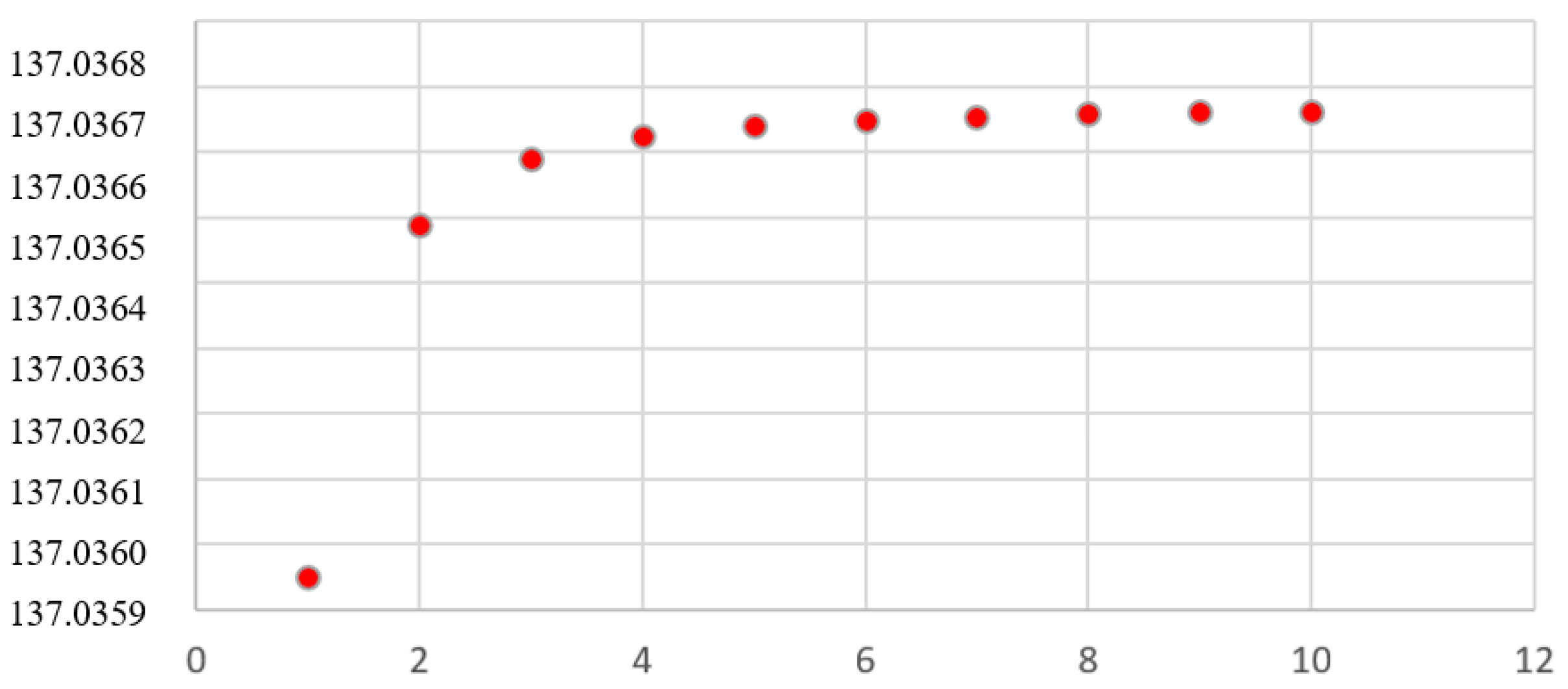
Table 1.
Sommerfeld Orbital Constants for Z = 1 (*).
| 1 | 137.035950244954 | 0.00729735517003008 |
| 2 | 137.036489933615 | 0.00729732643097056 |
| 3 | 137.036589876262 | 0.00729732110893124 |
| 4 | 137.036624856212 | 0.00729731924621806 |
| 5 | 137.036641046931 | 0.00729731838404832 |
| 6 | 137.036649841891 | 0.00729731791570920 |
| 7 | 137.036655144977 | 0.00729731763331538 |
| 8 | 137.036658586883 | 0.00729731745003099 |
| 9 | 137.036660946637 | 0.00729731732437210 |
| 10 | 137.036662634565 | 0.00729731723448852 |
(*) Values of the Sommerfeld constant for levels 1-10 were calculated for hydrogen using the recursive numerical method for electron capture presented in Ref. [10]. See Appendix A.
Table 2.
Sommerfeld Orbital Constants for Z = 2 (*).
| 1 | 137.034935840356 | 0.00729740918888733 |
| 2 | 137.036316427785 | 0.00729733567033653 |
| 3 | 137.036350014072 | 0.00729733388182998 |
| 4 | 137.036489934089 | 0.00729732643094532 |
| 5 | 137.036554696630 | 0.00729732298227863 |
| 6 | 137.036589876262 | 0.00729732110893124 |
| 7 | 137.036611088587 | 0.00729731997935612 |
| 8 | 137.036624856240 | 0.00729731924621657 |
| 9 | 137.036634295241 | 0.00729731874358161 |
| 10 | 137.036641046943 | 0.00729731838404768 |
(*) Values of the Sommerfeld constant for levels 1-10 were calculated for helium using the recursive numerical method for electron capture presented in Ref. [10]. See Appendix A.
Table 3.
Sommerfeld Orbital Constants for Z = 3 (*).
| 1 | 137.030194061221 | 0.00729766170770531 |
| 2 | 137.035050769958 | 0.00729740306864051 |
| 3 | 137.035950244954 | 0.00729735517003008 |
| 4 | 137.036265063006 | 0.00729733840556895 |
| 5 | 137.036410779106 | 0.00729733064602762 |
| 6 | 137.036489933615 | 0.00729732643097056 |
| 7 | 137.036537661315 | 0.00729732388942498 |
| 8 | 137.036568638438 | 0.00729732223986456 |
| 9 | 137.036589876262 | 0.00729732110893124 |
| 10 | 137.036605067546 | 0.00729732029998186 |
(*) Values of the Sommerfeld constant for levels 1-10 were calculated for lithium using the recursive numerical method for electron capture presented in Ref. [10]. See Appendix A.
Table 4.
H I Energy Levels (, , ).
| n | Theoretical (cm-1) |
Experimental (1) (cm-1) |
Th/Ex |
|---|---|---|---|
| 1 | 0.0000 | 0.0000 | - |
| 2 | 82262.1663 | 82258.9544 | 1.00003905 |
| 3 | 97495.2178 | 97492.3040 | 1.00002989 |
| 4 | 102826.7354 | 102823.9040 | 1.00002754 |
| 5 | 105294.4575 | 105291.6570 | 1.00002660 |
| 6 | 106634.9462 | 106632.1681 | 1.00002605 |
| 7 | 107443.2178 | 107440.4508 | 1.00002575 |
| 8 | 107967.8168 | 107965.0568 | 1,00002556 |
| 9 | 108327.4801 | 108324.7253 | 1.00002543 |
| 10 | 108584.7450 | 108581.9945 | 1.00002533 |
(1) NIST ASD Energy levels for Hydrogen.
Table 5.
D I Energy Levels (, , ).
| n | Theoretical (cm-1) |
Estimated (1) (cm-1) |
Th/Es |
|---|---|---|---|
| 1 | 0.0000 | 0.0000 | - |
| 2 | 82262.14406 | 82281.493 | 0.99976484 |
| 3 | 97495.19143 | 97518.836 | 0.99975754 |
| 4 | 102826.7076 | 102851.878 | 0.99975527 |
| 5 | 105294.4291 | 105320.308 | 0.99975428 |
| 6 | 106634.9174 | 106661.1812 | 0.99975376 |
| 7 | 107443.1888 | 107469.6848 | 0.99975346 |
| 8 | 107967.8169 | 107994.4344 | 0.99975326 |
| 9 | 108327.4800 | 108354.2009 | 0.99975312 |
| 10 | 108584.7156 | 108611.5396 | 0.99975308 |
(1) NIST ASD Energy levels for Deuterium.
Table 6.
He II Energy Levels (, ).
| n | Theoretical (cm-1) |
Estimated (1) (cm-1) |
Th/Es |
|---|---|---|---|
| 1 | 0.0000 | 0.0000 | - |
| 2 | 329193.15040 | 329179.76231 | 1.000041 |
| 3 | 390144.57400 | 390140.82497 | 1.000010 |
| 4 | 411476.97043 | 411477.18175 | 1.000000 |
| 5 | 421350.68083 | 421352.70920 | 0.999995 |
| 6 | 426714.14026 | 426717.15366 | 0.999993 |
| 7 | 429948.12435 | 429951.72607 | 0.999992 |
| 8 | 432047.09926 | 432051.07855 | 0.999991 |
| 9 | 433486.14721 | 433490.38252 | 0.999990 |
| 10 | 434515.48857 | 434519.90514 | 0.999990 |
(1) NIST ASD Energy levels for He II with relative abundance of 3He and 4He.
Table 7.
Li III Energy Levels (, ).
| n | Theoretical (cm-1) |
Estimated (1) (cm-1) |
Th/Es |
|---|---|---|---|
| 1 | 0.0000 | 0.0000 | - |
| 2 | 741001.31102 | 740736.43390 | 1.000358 |
| 3 | 878168.40029 | 877919.74441 | 1.000283 |
| 4 | 926172.79499 | 925932.85143 | 1.000259 |
| 5 | 948391.25468 | 948155.58428 | 1.000249 |
| 6 | 960460.35118 | 960226.99032 | 1.000243 |
| 7 | 967737.57099 | 967505.57339 | 1.000240 |
| 8 | 972460.74048 | 972229.60574 | 1.000238 |
| 9 | 975698.91808 | 975468.36035 | 1.000236 |
| 10 | 978015.16155 | 977785.00701 | 1.000235 |
(1) NIST ASD Energy levels for Li III with relative abundances of 6Li and 7LI.
Table 8.
H I Emission Lines - Lyman Series (, , ).
| Theoretical Exact (nm) |
Th. with slippage | Exp. (1) | |
|---|---|---|---|
| 10-1 | 92.09396771 | 92.0947 | 92.0947 |
| 9-1 | 92.31267996 | 92.3148 | 92.3148 |
| 8-1 | 92.62019267 | 92.6249 | 92.6249 |
| 7-1 | 93.07241725 | 93.0751 | 93.0751 |
| 6-1 | 93.77788760 | 93.7814 | 93.7814 |
| 5-1 | 94.97176049 | 94.9742 | 94.9742 |
| 4-1 | 97.25097237 | 97.2517 | 97.2517 |
| 3-1 | 102.56913342 | 102.5728 | 102.5728 |
| 2-1 | 121.56256576 | 121.5670 | 121.5670 |
(1) NIST ASD Spectra lines for Hydrogen – Lyman series.
Table 9.
H I Emission Lines – Balmer Series (, , ).
| Theoretical Exact (nm) |
Th. with slippage | Exp. (6) | |
|---|---|---|---|
| 10-2 | 379.901988789 | 379.7909 | 379.7909 |
| 9-2 | 383.651625364 | 383.5397 | 383.5397 |
| 8-2 | 389.019526145 | 388.9064 | 388.9064 |
| 7-2 | 397.124003794 | 397.0075 | 397.0075 |
| 6-2 | 410.293779975 | 410.1734 | 410.1734 |
| 5-2 | 433.173044477 | 434.0472 | 434.0472 |
| 4-2 | 486.273257938 | 486.1350 | 486.1350 |
| 3-2 | 656.46728858 | 656.2790 | 656.2790 |
(1) NIST ASD Spectra lines for Hydrogen – Balmer series.
Table 10.
H I Emission Lines - Paschen Series (, , ).
| Theoretical Exact (nm) | Th. with slippage | Exp. (1) | |
|---|---|---|---|
| 10-3 | 901.75169733 | 901.5300 | 901.5300 |
| 9-3 | 923.16819091 | 922.9700 | 922.9700 |
| 8-3 | 954.87279912 | 954.6200 | 954.6200 |
| 7-3 | 1005.22717686 | 1004.9800 | 1004.9800 |
| 6-3 | 1094.12441164 | 1093.8170 | 1093.8170 |
| 5-3 | 1282.17625443 | 1281.8072 | 1281.8072 |
| 4-3 | 1875.63856352 | 1875.1300 | 1875.1300 |
(1) NIST ASD Spectra lines for Hydrogen – Paschen series.
Table 11.
H I - Correction Ratio.
| 1-2 | 1.000054838 | - | - | - | - |
| 1-3 | 1.000143000 | 2-3 | 0.99982067 | - | - |
| 1-4 | 1.000056150 | 2-4 | 0.99957331 | 3-4 | 0.99989454 |
| 1-5 | 1.000308300 | 2-5 | 0.99923863 | 3-5 | 0.99974404 |
| 1-6 | 1.000655400 | 2-6 | 0.99882536 | 3-6 | 0.99957835 |
| 1-7 | 1.000691800 | 2-7 | 0.99834800 | 3-7 | 0.99945350 |
| 1-8 | 1.001600000 | 2-8 | 0.99781600 | 3-8 | 0.99919060 |
| 1-9 | 1.000918500 | 2-9 | 0.99718730 | 3-9 | 0.99914100 |
| 1-10 | 1.000394000 | 2-10 | 0.99648380 | 3-10 | 0.99875600 |
Table 12.
Hydrogen Atomic Constants.
| Atomic Constants Electron Capture Model |
Symbol - Equation | Theoretical Estimation (S.I.) |
|---|---|---|
| Mean square length | 1.27555662 | |
| Structure constant | 137.035950 | |
| Bohr radius (+) | 5.29162744 10-11 m | |
| Orbital radius | - | |
| Rydberg Constant (#) | 1.09737433 107 m-1 | |
| Rydberg Energy (#) | 13.6057028 eV |
(+) Theoretical values calculated during capture process. (#) Refers to the electrons captured in the hydrogen atom being stabilized.
Table 13.
He II - Emission Lines - Lyman Series (, ).
| Th. Exact (nm) |
Th. with slippage | Ritz (1) | ||
|---|---|---|---|---|
| 6-1 | 23.4348924878197 | 0.99987710544 | 23.43472796 | 23.43472796 |
| 5-1 | 23.7332000516591 | 0.99994308262 | 23.73308751 | 23.73308751 |
| 4-1 | 24.3026966721836 | 0.99999722314 | 24.30268767 | 24.30268767 |
| 3-1 | 25.6315239693052 | 1.0000384430 | 25.63177027 | 25.63177027 |
| 2-1 | 30.3773027712290 | 1.0000631456 | 30.37858147 | 30.37858147 |
(1) NIST ASD Spectra lines for Hydrogen He II – Lyman series.
Table 14.
Li III - Emission Lines - Lyman Series (,).
| Th. Exact (nm) |
Th. With slippage | Exp. (1) | ||
|---|---|---|---|---|
| 8-1 | 10.2831914788377 | 1.02300 | 10.29 | 10.29 |
| 7-1 | 10.3333799366446 | 1.01600 | 10.34 | 10.34 |
| 6-1 | 10.4116739308196 | 0.99800 | 10.41 | 10.41 |
| 5-1 | 10.5441714594132 | 1.00800 | 10.55 | 10.55 |
| 4-1 | 10.7971212866958 | 1.00200 | 10.80 | 10.80 |
| 3-1 | 11.3873375502246 | 1.00100 | 11.39 | 11.39 |
| 2-1 | 13.4952527765271 | 1.00055 | 13.50 | 13.50 |
(1) NIST ASD Spectra lines for Lithium Li III – Lyman series.
Disclaimer/Publisher’s Note: The statements, opinions and data contained in all publications are solely those of the individual author(s) and contributor(s) and not of MDPI and/or the editor(s). MDPI and/or the editor(s) disclaim responsibility for any injury to people or property resulting from any ideas, methods, instructions or products referred to in the content. |
© 2024 by the authors. Licensee MDPI, Basel, Switzerland. This article is an open access article distributed under the terms and conditions of the Creative Commons Attribution (CC BY) license (http://creativecommons.org/licenses/by/4.0/).
Copyright: This open access article is published under a Creative Commons CC BY 4.0 license, which permit the free download, distribution, and reuse, provided that the author and preprint are cited in any reuse.


