
Submitted:
04 July 2024
Posted:
05 July 2024
You are already at the latest version
Abstract
Advanced 1H Nuclear Magnetic Resonance (NMR) relaxometry and diffusometry methods and VIS-nearIR spectroscopy combined with pH, electric conductivity (EC) and totally dissolved solids (TDS) measurements were used to assess the properties of wastewater collected from a chicken slaughterhouse in each step of the treatment process (wastewater before treatment, biologically treated wastewater, chemically treated wastewater and discharged wastewater) and from sludge. The 1H NMR Carr-Purcell-Meiboom-Gill (CPMG) and Pulsed-Gradient-Stimulated-Echo (PGSE) decay curves recorded for all samples of wastewater were analyzed by inverse Laplace transform (ILT) to obtain the distributions of transverse relaxation times T2 and diffusion coefficient D. The VIS-nearIR total absorbance, T2-values, D-values, pH, EC and TDS parameters were used for statistical analysis in principal component analysis (PCA). The 1H T2-distributions measured for the slaughterhouse wastewater lie in two main regions reflecting the amount of dissolved solids or the distribution of undissolved solids mobility. The PCA analysis successfully differentiates between polluted and less polluted types of wastewater and sludge. The wastewater treatment applied by the slaughterhouse is efficient. The recommended methods for wastewater monitoring are the NMR T2- and D-distributions and EC, TDS and NMR-D diffusion coefficient. Finally, Machine Learning AI-algorithms are used to provide prediction maps of wastewater treatment stage.
Keywords:
Slaughterhouse wastewater and sludge
; 1H NMR relaxometry and diffusometry
; VIS-nearIR spectroscopy
; pH
; EC and TDS measurements
; PCA-principal component analysis
; AI-prediction using Machine Learning
1. Introduction
Nuclear Magnetic Resonance (NMR) is a powerful analytical tool, extensively used in the characterization of microscopic properties of many classes of materials. Though, it is not yet favored in the assessment of wastewater properties, in particular of that collected from slaughterhouses. Classical measurements of wastewater characteristics are mainly based on determining the physicochemical global parameters such as: electrical conductivity (EC), total suspended solids (TSS), total dissolved solids (TDS), apparent color, turbidity, pH, chemical oxygen demand (COD) and ammoniacal nitrogen (NH3-N) of poultry slaughterhouse wastewater (PSW) [1]. The distilled water has a poor electric conductivity due to the lack of ions. The presence of electrically charged particles is necessary to support the electrical conduction in solutions. Therefore, measuring a high electric conductivity in wastewater is clearly indicating the presence of various types of particles, and thus of a certain degree of wastewater pollution [2]. Determining the total suspended solids (TSS) and the total dissolved solids (TDS) can indicate the amount of undissolved solid pollutants and that of dissolved pollutants, respectively. The TDS and/or the TSS values are usually proportional to the amounts of these solids in the aqueous sample. Depending on the size and on the electrical properties of the particles in the wastewater, the liquid presents certain sensitivity to the incident light. Therefore, an apparent color of wastewater can be associated to the presence of specific pollutants. Otherwise, the overall characterization within the visible range can be done by performing turbidity measurements. The presence of dissolved or undissolved pollutants increases its turbidity and therefore reduces the intensity of light transmitted through wastewater samples [3]. Water is a good solvent for a large range of compounds. Therefore, the measurement of wastewater pH value can indicate the pollution level [4,5]. The amount of organic matter in wastewater samples can be determined by classical methods such as: i) the total organic carbon (TOC), directly indicating the organic matter content; ii) biochemical oxygen demand (BOD), and iii) chemical oxygen demand (COD) measurements. The last two offer an indirect quantification of the total organic matter content in aqueous samples. The biochemical oxygen demand is related to the biodegradable organic content of samples. This can be quantified by measuring the oxygen consumption by microorganisms present in the water samples [6,7]. Another indicator of the total organic content is the presence of ammonia, an inorganic compound that demands and consumes oxygen during the process of conversion to nitrate.
Throughout all the stages in the slaughterhouse production line, large amounts of water are consumed (15-20 l/chicken), thus also requiring an intense processing of wastewater used in the poultry industry. This is loaded with organic matters that may re-enter in the environment in large amounts, via effluents [1,8]. It is therefore essential to apply efficient purification treatments of wastewaters prior to be released. The wastewater management is considered an important task, subjected to strict global regulations [9,10,11]. Some well-established physicochemical methods, used to treat the wastewater, by removing contaminants such as metals, organic matter (OM) and total suspended solids, are [12]: coagulation–flocculation [13,14]; flotation [15,16]; electrocoagulation [17,18]; chemical precipitation [1,13,19,20,21]; ultra- and nano-membrane filtration and reverse osmosis [22,23]. Traditionally, biological (aerobic and anaerobic) treatment methods have been used for poultry slaughterhouse wastewater treatment. Unfortunately, both biological techniques present some limitations [24]. The conventional treatment processes of agro-industrial wastewater based on the aerobic technologies requires high energy consumption for aeration and generates large amounts of sludge. In recent years, these tend to be replaced by more environmental friendly anaerobic biotechnologies. Among others, for the slaughterhouse wastewaters treatment, the sequencing batch reactor (SBR) showed a good efficiency of pollutants removal.
NMR is one of the most used characterization methods for a large variety of materials, from plastics to elastomers [25,26,27,28], ordered tissues [29,30], tissue regeneration (e.g. in Albino Wistar rats femurs and sciatic nerve) [31,32,33,34,35], denaturation of keratin [36,37], proton exchange membranes [38,39], corn starch [40,41], construction materials [42,43] or even for in vivo human tissues (e.g. healthy woman uterus) [44]. With the exception of plastic/elastomers, for all other materials the 1H NMR implies the study of water states. The H2O is seen as “spy” molecules in interaction with organic and inorganic materials. A logical step was to apply the well-known 1H NMR such as: i) one-dimensional 1H NMR relaxometry to obtain the transverse relaxation times T2-distribution, sensitive to water pools dimension [9,31,32,33,34,35,40,41,42,43,44,45,46]; ii) one-dimensional 1H NMR diffusometry to obtain the distribution of self-diffusion coefficient D, sensitive to molecular water mobility and water pools restrictions [38,39]. These two NMR parameters are sensitive to water impurities, and thus different water components can be revealed. For example, in slaughterhouse wastewater it can be found: i) soluble impurities that will increase the wastewater viscosity reducing the T2 and D values or ii) insoluble impurities that, depending on their dimensions, can be seen as different relaxation environments leading to multiple T2-values. Having different sizes and different hydrophilicity (or hydrophobicity) such impurities can act (or not) as transport vehicles for water molecules. Then, one can observe multiple values in the measured D-distribution. The NMR data are analyzed by the inverse Laplace transform (ILT) [47,48,49,50]. In this way one can obtain the distribution of relevant NMR parameters to describe the wastewater states by water components [9,27,28,32,33,34,35,39,40,41,42,43,45,46,51,52,53,54].
The aim of this study is to assess the efficiency of new methods such as low field 1H NMR relaxometry and diffusometry, VIS-nearIR spectroscopy in analyzing the polluted wastewater (PSW) during treatment process in the slaughterhouse. The advantage of these methods resides in their ability to offer a large range (distribution) of the measured parameters. The sample apparent color is used to characterize the wastewater contamination with impurities. Such soluble or insoluble impurities can increase the turbidity of wastewater samples. In this study we aim to better characterize these two parameters by VIS-nearIR spectra measured for a domain of wavelengths from 390-980 nm. Afterwards, we show how the non-classical methods can be combined with the classical ones which characterize the entire wastewater samples, for a complex analysis in Principal Component (PCA) [55,56]. The PCA statistical data leads to graphic plots that are easily interpreted to discriminate between all types of wastewater (at least between the polluted and less polluted). Thus, the PCA can be used to evaluate the treatment process efficiency and can offer information about the relevance of each measured parameter in the characterization of the PSW purification. Moreover, it can be used in combination with machine learning algorithms to provide prediction related to of the stage of the treatment process.
2. Materials and Methods
2.1. Materials and Processes in the Slaughterhouse Wastewater Purification Treatment
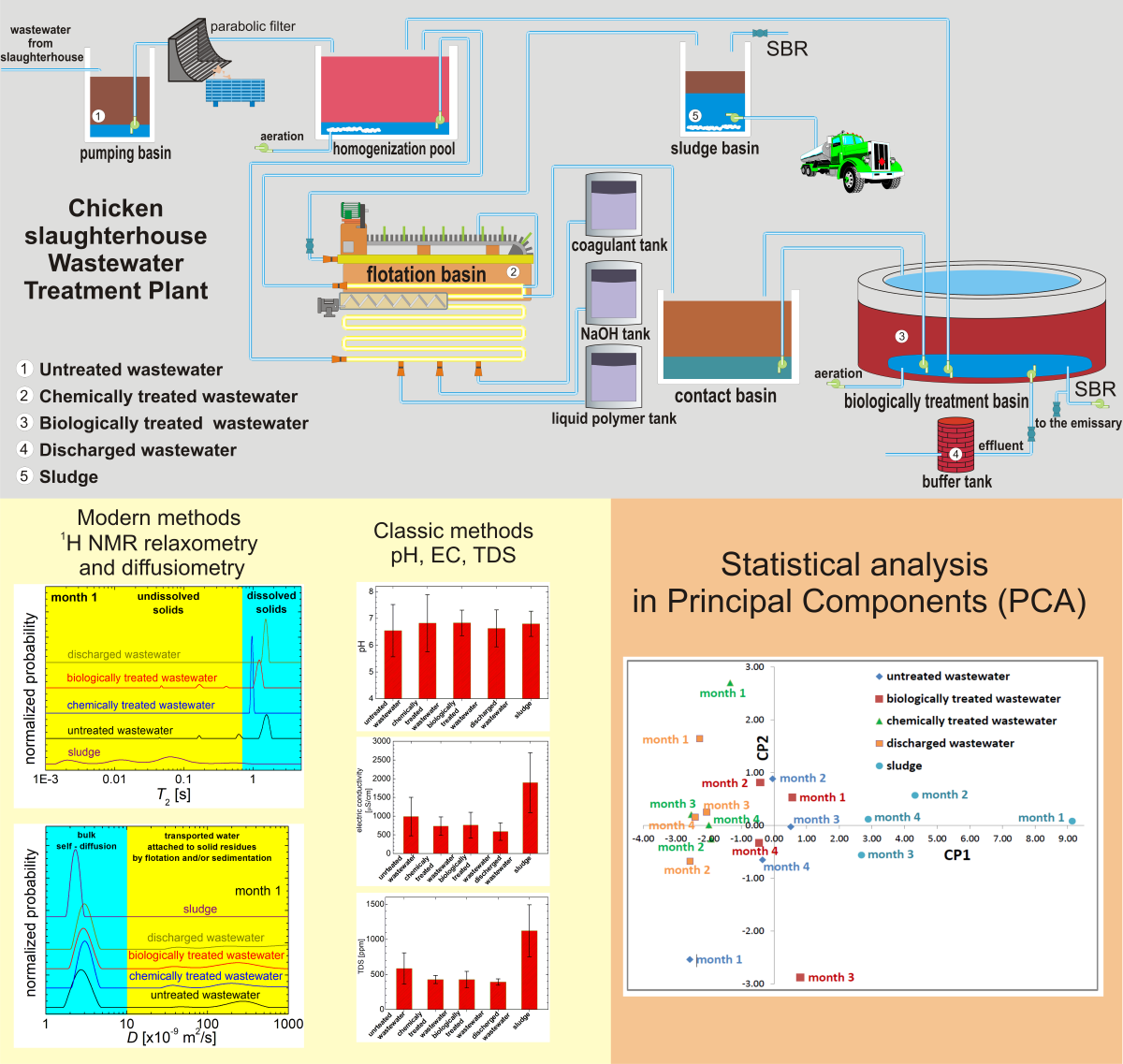
The wastewater and sludge samples were collected from a chicken slaughterhouse located in the north-western part of Romania, from winter to spring in four different months. The main components of chicken slaughterhouse purification treatment plant are presented in Figure 1. The untreated wastewater was collected from the pumping basin where the wastewater is brought directly from the slaughterhouse. This wastewater contains all the specific organic matter pollutants resulted from slaughterhouse, such as: dejection, fodder, gastric contents, blood, fragments of meat and intestines, fats, feather remnants, etc. From here, the wastewater is pumped on a parabolic filter that allows to pas only the wastewater and small particles while the large residues are collected by gravitation, in an external tank (see Figure 1). Next, the wastewater is stored in a large pool, where it is periodically mixed by aeration, to avoid the sedimentation of heavy matter. From here, the wastewater is pumped in a flotation basin for chemical treatment. This treatment is performed in the presence of SUPERFLOC C-2240 (registered trademark) liquid cationic polymer. According to the producers, this liquid coagulant polymer acts as primary coagulant being a charge neutralization agent in the liquid/solid separation processes. The liquid polymer enables the filtration, flotation of dissolved air, wastewater clarification, and reduces the use of inorganic salts. It is used at a ratio of approximately 1.8 l of liquid polymer to 1000 l of wastewater, but the effective dose is pH controlled.
The second chemical agent is sodium hydroxide (NaOH), popularly known as caustic soda (or lye). This is a highly caustic base, used to decompose the proteins remained in the wastewater. Ferric sulphate is the third chemical agent, typically used for wastewater treatment and sludge conditioning, for removing phosphorus, to reduce the hydrogen sulphate, to attenuate the corrosiveness and odor of wastewater and sludge.
Figure 1.
The main components of the wastewater purification treatment plant of a chicken slaughterhouse.
Figure 1.
The main components of the wastewater purification treatment plant of a chicken slaughterhouse.
Being lighter than water, the coagulated sludge, is collected from the wastewater surface in the flotation basin with a paddled conveyer belt, and is stored in a sludge basin. From here it is then transported to another city to be used in producing biogas.
The sludge samples were collected from the sludge basins as shown in Figure 1. The chemically treated wastewater samples were collected from the bottom of the flotation basin through a drain hole (see Figure 1). After its separation from sludge, the chemically treated wastewater is pumped in the contact tank that communicates with an external basin where the liquid undergoes the biologically treatment process. This is mainly based on the anaerobic bacterial treatment in a classical sequencing batch reactor (SBR) also shown in Figure 1. In this biological treatment basin, the bacterial population is controlled by wastewater retraction in the contact basin and/or by aeration. The samples of biologically treated wastewater were collected in the daylight during the purification process. The bio-purification technology implies numerous steps. To be discharged after a sequence of nitrification, the wastewater is subjected to a 2 h stage of nitro-sedimentation, followed by another 2 h stage of sedimentation. The control mechanism of the wastewater station only allows the wastewater to be discharged after these 4 hours of sedimentation stage, which usually takes place overnight. The samples of discharged, and hence completely treated wastewater, were collected from a buffer tank located between the slaughterhouse treatment plant and the Crasna River flowing nearby. The sediments collected at the bottom of the biological treatment basin are pumped back in the homogenization pool, and re-enter to the purification circuit, undergoing again the chemical treatment and separation from sludge in the flotation basin. Thus, the sludge results from combined both the biological and the chemical treatments.
The wastewater samples (untreated wastewater, chemically treated wastewater, biologically treated wastewater, discharged wastewater) and sludge were stored each in ½ l plastic containers, immediately transported to the analytical laboratory in the Technical University of Cluj-Napoca (TUCN) and the analyses run as soon as possible. Prior to each measurement, the samples were homogenized by manually agitating the bottles for 1-3 minutes. Between the successive sets of measurements the wastewater samples were stored in the transport bottles at room temperature and protected from light.
2.2. Methods
The first set of measurements where performed for the overall parameters: pH, electric conductivity and totally dissolved solids (TDS). The second set of measurements consisted of the 1H NMR relaxometry that lasted several minutes per measurement. The 1H NMR diffusometry measurements were the longest, lasting approximately 80 minutes per sample. Finally the FT-IR spectra (not discussed here) were the last performed measurements, requiring in total 5 minutes per sample [9].
The 1H NMR relaxometry and diffusometry measurements for all the wastewater samples were performed using a Bruker Minispec MQ 20 spectrometer working at 19.69 MHz. The NMR relaxation data were recorded using the well-known CPMG (Carr-Purcell-Meiboom-Gill) pulse sequence [9,27,28,31,32,33,34,35,40,41,42,43] with echo time 2τ = 2 ms (Figure SI 1a, in the Supplementary Information). A total of 3000 echoes were registered, and the repetition time or recycle delay (RD) was set at 3 s. For a good signal to noise ratio (Figure 2a), acquiring 32 scans was sufficient [9]. Then, the experimental data were processed using a fast inverse Laplace-like transform (ILT) algorithm, increasingly used in recent years to analyze multi-exponential decay curves [9,27,28,31,32,33,34,35,40,41,42,43,46,47,48,49,50]. The NMR self-diffusion data were recorded using the pulsed gradient stimulated echo (PGSE) pulse sequence (Figure SI 1b in the Supplementary Information). The inter echo time τ was set at 3 ms, the encoding and decoding pulse gradients duration δ was 0.4 ms, while the self-diffusion time Δ was set at 20 ms. A number of 64 acquisitions were collected with a recycle delay of 1.5 s. The recorded data were analyzed by the ILT algorithm with the proper (see below) kernel. The ILT analysis [47,48,49,50] will be described in paragraph 2.3 below.
The Vis-nearIR spectra were recorded in less than 10 seconds per sample, using a PASCO spectrometer. For some wastewater samples a sedimentation time was necessary before each measurement. The sludge samples were distilled in a ratio of 1:20, by adding 1 ml sludge to 20 ml of distilled water. The measurements set-up were as follow: i) the lower wavelength λL was 379.928 nm; ii) the higher wavelength λH was 950.11 nm; iii) a total number of 2132 points were acquired with a resolution of 0.268 nm; iv) 25 scans were accumulated to increase the signal to noise ratio (SNR).
The pH and the electric conductivity were measured using a water quality meter multi-parameter Model 8603. The totally dissolved solids were measured using a pocket TDS/EC meter. All the methods of measurement/analysis follow the standard protocols [1].
2.3. Data Analysis
The CPMG decays of nuclear magnetization, M(tCPMG) characteristic to water with many types of impurities (see Figure 2a) are assumed to be multi-exponential. Each specific transverse relaxation time describes a certain spin dynamics according to the 1H environment. Therefore, the M(tCPMG) decay can be written as [41,42,43,44,45,46,47,48,49,50]:
where the P(T2,i) is the probability to find a statistical spin ensemble (water 1H) characterized by a specific transverse relaxation time T2,i [31,34,42]. The tCPMG = τ2 = 2nτ is the total duration of the CPMG experiment, as can be seen from figure SI 1a in Supplementary Information. To consider a real distribution of transverse relaxation times, the decay of the nuclear magnetization presented in eq. (1) can be considered to have an integral Laplace-like form that also contains the distribution function of transverse relaxation times f(T2) [41,42,43,44,45,46,47,48,49,50]:
Nevertheless, the practical way to analyze the discretized acquired NMR signal is to combine the finite summation presented in eq. (1) and the distribution function f(T2). Finally, the goal of an inverse Laplace analysis is to find a normalized distribution function f(T2). This will be interpreted as normalized probability to find a statistically relevant number of water 1H characterized by a particular value of T2. Here we have to remark that the transverse relaxation process assumes a certain loss of phase of the nuclear spins precessing around a static magnetic field and at the same time being in interaction with neighboring spins. Therefore, for just an isolated spin the T2 is not defined.
Similarly, the decay of the normalized pulsed field gradient echo (PGSE) NMR signal can be viewed in an integral Laplace-like form containing the specific distribution function f(D) of the self-diffusion coefficient [39,48]:
where D is the self-diffusion coefficient and the distribution function f(D) is the parameter function to be obtained. The new kernel of Laplace-like integral presented in eq. (3) contains the 1H gyromagnetic ratio γ; the magnetic field gradient strength g; the duration of encoding/decoding pulsed gradients δ and the self-diffusion time Δ.
2.4. Statistical Analysis
In general it is not possible to directly compare the behavioral effects of two parameters of different types. Though, there exists a standard method largely used to analyze the statistical data (usually from more than one group) that are characterized by numerous variables or observables having different measurement units. This is the multivariate analysis, in particular the principal components analysis (PCA) [28]. For our study, we implemented our own numerical program in Matlab and we plotted the results in Microsoft Excel software. For such PCA statistical analysis, a data matrix is produced containing the input values that will be discussed later in Table 1. As variables, we selected: i) the total absorbance from the Vis-nearIR spectra; ii) the most probable transverse relaxation time T2,1 characteristic to wastewater with dissolved solids, from 1H NMR relaxometry measurements; iii) the most probable self-diffusion coefficient D1 specific also to wastewater with dissolved solids, from 1H NMR diffusometry measurements; and the bulk values for iv) pH; v) electric conductivity (EC) and vi) totally dissolved solids (TDS). All the values of these six parameters were considered for all our five groups of four samples, each of them corresponding to one month monitoring. The values of these parameters form the input matrix with 6 columns and 20 rows. The results of the PCA method will be largely discussed later in the text.
2.5. Prediction Using Machine Learning ML5, an AI-Based Algorithm
The two-dimensional PC1-PC2 map obtained from PCA analysis were used for an advanced prediction of probability maps from any newly assumed measurements using the machine learning library ML5 [57,58]. For that, a dedicated program was written in JavaScript following the descriptions presented in ref. [58] and adapted for our purpose. The 20 (=5 × 4) values obtained from PCA analysis was used to train an Artificial Neural Network (ANN) with a learning rate of 10% and for 10000 epochs. The resulted model was saved and reloaded to predict the probability that a new measurement, located on each element of a 100 × 100 matrix correlated to the PC1-PC2 map obtained from the PCA analysis, to be associated to each type of wastewater or sludge.
3. Results
3.1. 1H NMR Relaxometry of Wastewater and of Sludge from the Chicken Slaughterhouse
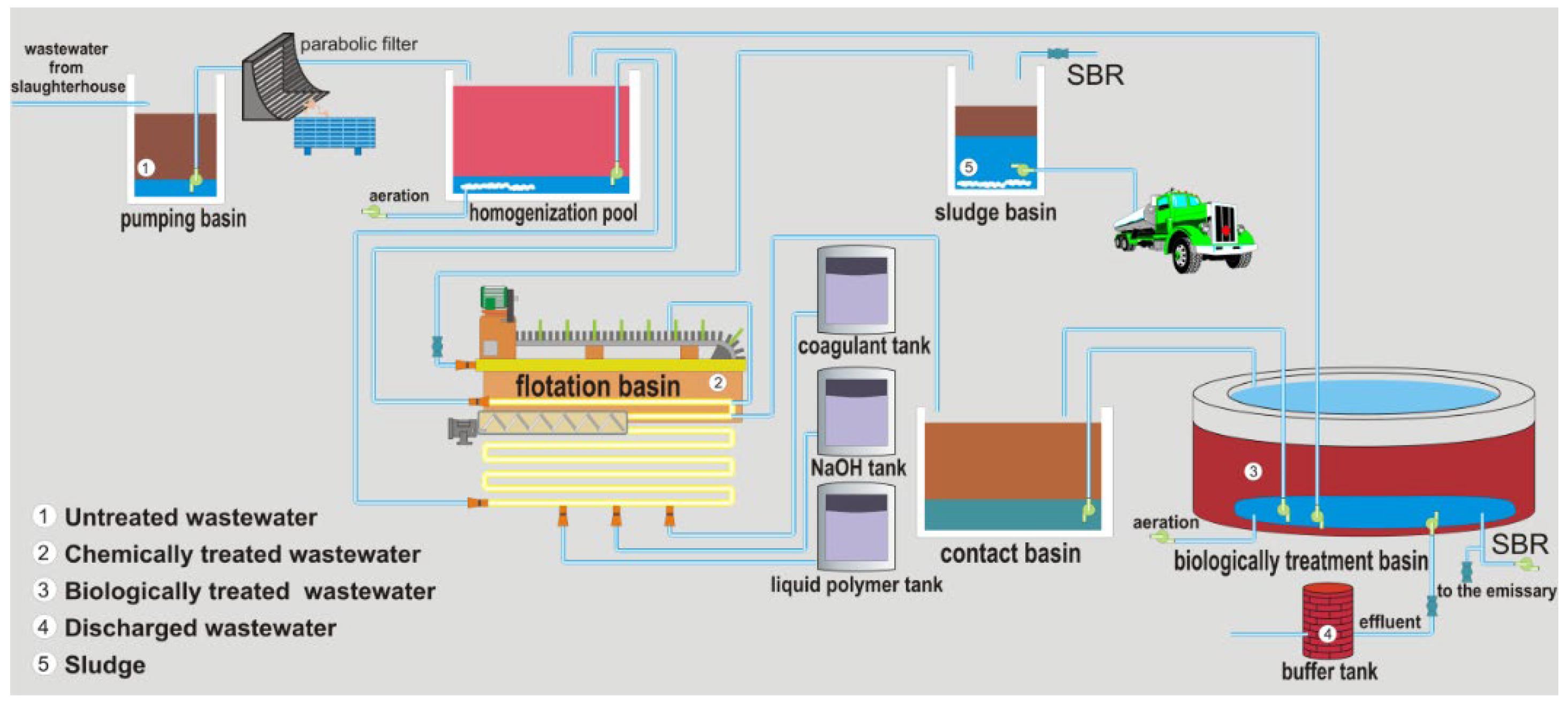
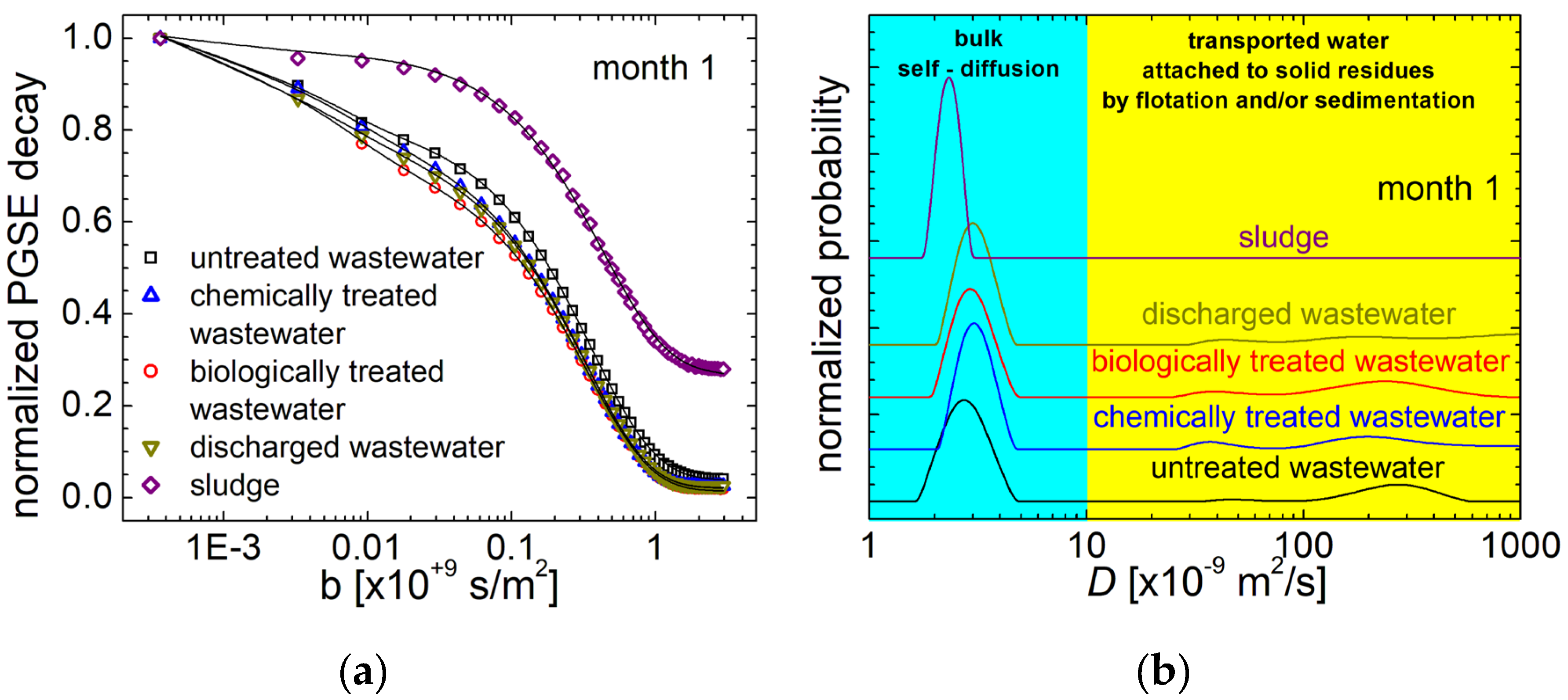
The results obtained by measuring the normalized 1H nuclear magnetization decays during the CPMG pulse sequence for all types of wastewater and sludge samples collected over the first month of monitoring, are compared in Figure 2a. At 6 seconds a complete decay (less than 5% from initial magnetization) is observed for all the wastewater samples, indicating a large mobility of water molecules. An equivalent decay is observed for sludge (purple diamond in Figure 2a) but this is achieved in less than 0.2 s indicating, as expected, a strong mobility limitation for the water molecules. Among wastewater samples the slowest decay was measured in discharged wastewater (dark yellow down triangle) that is expected to present the smallest amount of impurities. Chemically (blue up triangle) and biologically (red circle) treated wastewaters present the fastest decays suggesting the presence of large amounts of undissolved solids and/or dissolved solids, and/or the presence of paramagnetic impurities.
Figure 2.
(a) The normalized CPMG decays recorded for the slaughterhouse wastewater (untreated—black square, chemically treated—blue up triangle, biologically treated—red circle and discharged wastewater—dark yellow lower triangle) and sludge (diamonds) collected in month 1 of monitoring; (b) The normalized T2-distributions of the CPMG decay curves presented in (a).
A better analysis of the normalized 1H nuclear magnetization decays can be achieved by an inverse Laplace analysis [41,42,43,44,45,46,47,48,49,50]. The normalized transverse relaxation time T2-distributions obtained from ILT of CPMG decays measured for slaughterhouse wastewater (untreated, chemically and biologically treated and discharged wastewater) and for sludge are presented in Figure 2b. The normalized probability function f(T2) presents a series of peaks at different T2-values covering more than three orders of magnitude from 1 ms up to 3 seconds. From left to right (from small to large T2-values) these peaks can be associated with water molecules being in different environments. For example, the 1H with more restricted mobility are characterized by small T2-values, while water 1H with less restricted mobility are characterized by large T2-values. Considering the specificity of our samples, one can divide the full domain of T2-values in two main subdomains. Thus, there is the range of T2-values from 1 ms up to 700 ms, of water molecules attached to undissolved solids (on yellow background), and the subdomain of T2-values from 700 ms to 3 s (with blue-cyan background) where the particular position of peaks and therefore of the most probable T2-values is influenced by the type and amount of dissolved particles [9]. In particular, we measured for our low filed NMR spectrometer a T2-value for distilled water (no dissolved or undissolved particles) of 2.66 ± 0.1 s (see Figure 3). The presence of various dissolved solids should be then evaluated by taking into account this reference value. From Figure 2b, for wastewater samples in the subdomain of water pools with dissolved particles it can be observed only one peak but up to three peaks for water pools with undissolved particles. It is reasonable to assume that the water molecules are attached permanently or can experience a certain exchange between free water and bound water [39] and the attachment is to undissolved particles of different dimensions. The size (and shape, density, hydrophilicity/hydrophobicity) of such particles can influence the mobility of undissolved particles hence the mobility of water molecules attached to these particles. The NMR T2 relaxation time is sensitive to 1H mobility and therefore it is a good parameter to sense and characterize the presence and sizes of such undissolved particles. Furthermore, it is reasonable to assume the fact that large particles will have a small mobility and the corresponding T2 relaxation times values are also small. Small particles will have then a large mobility and a large corresponding T2-value. The integral area under the peaks, as it is measured from the T2-distributions, is proportional with the number of 1H present in each pool with a specific transverse relaxation time value.
Considering the above, in Figure 2b it can be observed that the T2-distributions measured for the untreated wastewater is characterized by four peaks: i) a large peak (the largest integral area under the peak) in the subdomain of water with dissolved solids with the most probable T2-value of 1.57 s not so far from the limit of 2.66 s (blue curve in Figure 3), indicating a small amount of dissolved solids; ii) a relative large peak centered at a T2-value of ~0.63 s indicating a large amount of small undissolved particles; iii) a relatively medium size peak centered at a T2-value of ~0.17 s indicating the presence of medium size undissolved particles and iv) a small (at the observable limit) peak centered at a T2-value of ~45 ms indicating the presence of relatively large undissolved particles. In general, 1H NMR relaxometry is a method capable, within certain limits, to also offer the size of such particles (or pores [42]), but the experiments need to be performed under more idealistic conditions for inorganic interface water-matter, where a certain surface relaxation parameter has to be estimated, conditions that are not fulfilled in our study. Furthermore, for untreated wastewater, the sampling procedure can play an essential role. For example, in our case the narrow bore pipette used to insert the sample in the NMR tube was acting as a filter for the larger undissolved fragments that are typically present in untreated wastewater.
The chemically treated wastewater (blue line in Figure 2b) is characterized by a single peak in the subdomains of water with dissolved solids. The fact that no peaks were found in the domain of water with undissolved solids is a good indicator of the efficiency of the coagulation-flotation sludge separation process applied in the chemical treatment basin. On the other hand, the most probable T2-value of ~0.96 s indicates a larger presence of dissolved solids compared with the T2-value of ~1.57 s measured for the untreated wastewater. Two processes could explain these findings: i) the undissolved solids subjected to chemical treatment became soluble in water and ii) the chemicals (liquid polymer, caustic soda and especially the ferric sulphate) enrich the water with paramagnetic impurities. The measured signal is the narrowest peak, compared to all the peaks measured for wastewater samples, also indicating a high degree of homogeneity of this sample. Surprisingly, the biologically treated wastewater is characterized again by four peaks, one in the subdomain of water with dissolved solids and three in the range of water with undissolved solids. At first glance this looks like a regress in the treatment process, but one must consider the complex mechanism of wastewater treatment presented in the Figure 1. This wastewater sample was collected from the biological treatment basin, in day light and in the presence of anaerobic bacteria, with nitrification and aeration processes that mixed all components, prior to the nitro-sedimentation and sedimentation. The peaks position in the T2-distributions measured for the biologically treated wastewater (red distribution function) for water with undissolved solids is almost identical to the position of the peaks obtained for untreated wastewater (black curve). A quality improvement of the water with dissolved solids can be noticed by observing that the most probable T2-value increases from ~0.96 s (measured for chemically treated wastewater) to ~1.24 s.
The efficiency in the pollutants removal by using this sequencing batch reactor (SBR) for the wastewaters treatment is observed from the T2-distributions measured for the discharged wastewater, after several hours allowing for nitro-sedimentation and sedimentation. The T2-distribution is characterized by a single peak located in the subdomain of water with dissolved solids at a T2-value of ~1.53 s. The position of this peak is similar with the position of the peak obtained for untreated wastewater sample in the subdomain of water with dissolved solids. Its narrower linewidth indicates less variation in the types of dissolved solids.
The sludge (purple distribution at the bottom of Figure 2b) also presents four peaks, but all of them are characterized by reduced T2-values, suggesting, as expected, the presence of protons with a reduced mobility. In fact, the term water with undissolved solids may by inappropriate in this case, since the sludge is a complex colloidal system [46]. Here a large amount of water is trapped to the organic and inorganic matters therefore have a reduced mobility and cannot be easily released. Moreover, taking into consideration the lower limit of T2-values (~2 ms) measured for this sample of slaughterhouse sludge, one can reasonably assume that this peak corresponds to the 1H from organic matter. The remaining peaks in the range of ~6 ms up to 1 s can be associated with water strongly bound to organic phase via vicinal water (hydrogen bound), with interstitial water physically trapped in bio-floc, by steric hindrance and with a small amount of water with higher mobility being less affected by the solid composition [45,46].
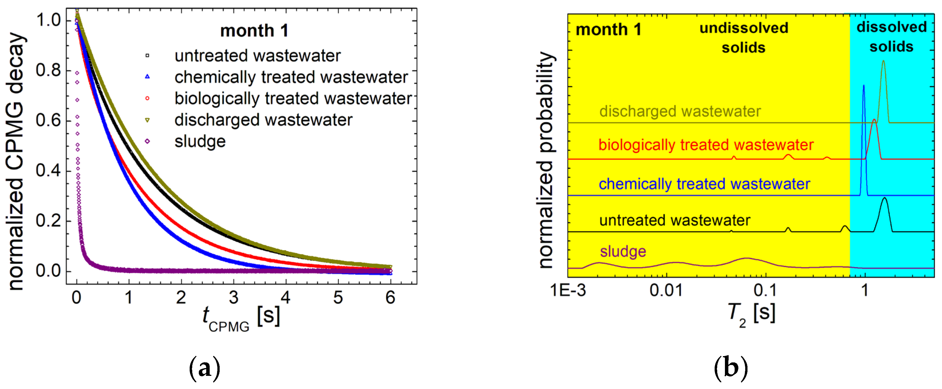
To assess the effect of specific solids on the T2-distributions measured for this slaughterhouse wastewater, three samples were prepared: i) distilled water; ii) distilled water with chicken feather rachis and iii) distilled water with chicken feather barb, proximal and distal barbule. The chicken feather was used as it was collected without additional purification by washing and/or sterilization. The measured T2-distributions for those three samples are presented in Figure 3. It can be observed that the sample of distilled water (blue distribution) presents a single peak with the most probable T2-value (maximum of peak) centered at 2.66 seconds. The T2-distributions measured for distilled water samples with parts of chicken feather present three peaks: i) the main broad peak (compared to the peak of pure distilled water) indicates an increased inhomogeneity of the aqueous medium; ii) a small peak located between ~0.8 to 1.3 seconds placed in the subdomain of water with dissolved solids indicates that part of feather impurities are dissolved in water and iii) a small peak located between ~0.16 and ~0.23 s, indicates a less restricted mobility. This can be associated with water attached to chicken feather parts. Also, this water may experience a certain exchange with free water, therefore the real T2-values may be affected by this exchange process [49]. As expected, due to smaller parts of feather such as barb, proximal and distal barbule compared to rachis, the T2-distributions measured for the first sample (top, red distribution in Figure 3) present broader peaks indicating a higher degree of inhomogeneity. Moreover, the position of the main peak is shifted towards smaller values indicating a reduction in the water mobility, most probably, by the interstitial water between barbs and barbules. In conclusion, these measurements demonstrates the effect of typical pollutants present in the chicken slaughterhouse wastewater, able to induce additional peaks at smaller T2-values in the T2-subdomains of water with undissolved solids (see Figure 2b), but also to shift the peaks located in the T2-subdomains of water with dissolved solids towards smaller T2-values.
Figure 3.
The normalized T2-distributions recorded for distilled water (bottom blue line), distilled water with chickens feather rachis (middle orange line) and distilled water with chicken feather barb and proximal and distal barbule (top red line).
Figure 3.
The normalized T2-distributions recorded for distilled water (bottom blue line), distilled water with chickens feather rachis (middle orange line) and distilled water with chicken feather barb and proximal and distal barbule (top red line).
The normalized T2-distributions recorded for four types of slaughterhouse wastewater (untreated, chemically treated, biologically treated and discharged water, respectively) collected during months 2, 3 and 4 are presented in Figure 4. As expected, the main characteristics of these T2-distributions are similar to those presented by samples collected in month 1, shown in Figure 2b, and discussed above. Nevertheless, the existence of some variability indicates the necessity for a statistical analysis of such samples. In this sense, for the T2-distributions collected during months 2 to 4, one can remark: i) the presence of two to three peaks for the untreated wastewater; ii) the presence of one or no-peak for the chemically treated wastewater; iii) two or three peaks for the biologically treated wastewater and iv) just one peak for the discharged wastewater which confirms the efficiency in the wastewater treatment applied.
Figure 4.
The normalized T2-distributions recorded for the slaughterhouse wastewater: untreated (black), chemically treated (blue), biologically treated (red) and discharged wastewater (dark yellow) collected in (a) month 2; (b) month 3; (c) month 4.
Figure 4.
The normalized T2-distributions recorded for the slaughterhouse wastewater: untreated (black), chemically treated (blue), biologically treated (red) and discharged wastewater (dark yellow) collected in (a) month 2; (b) month 3; (c) month 4.
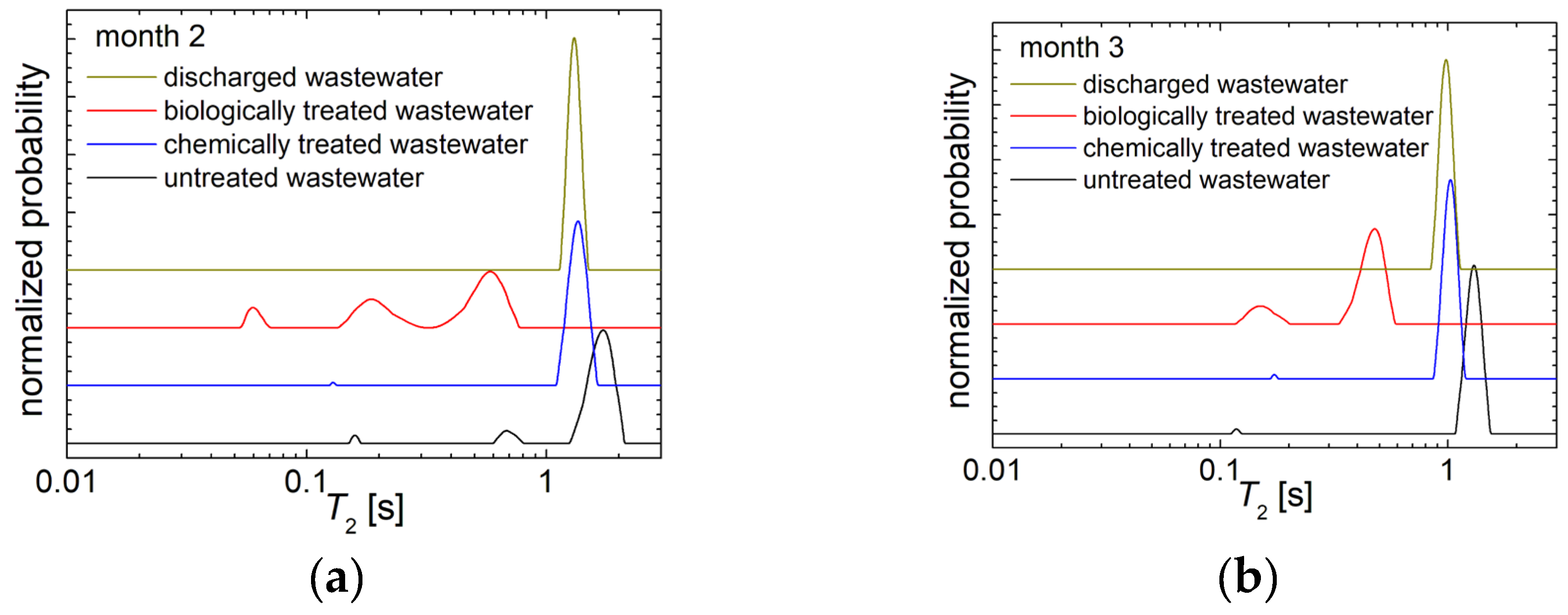
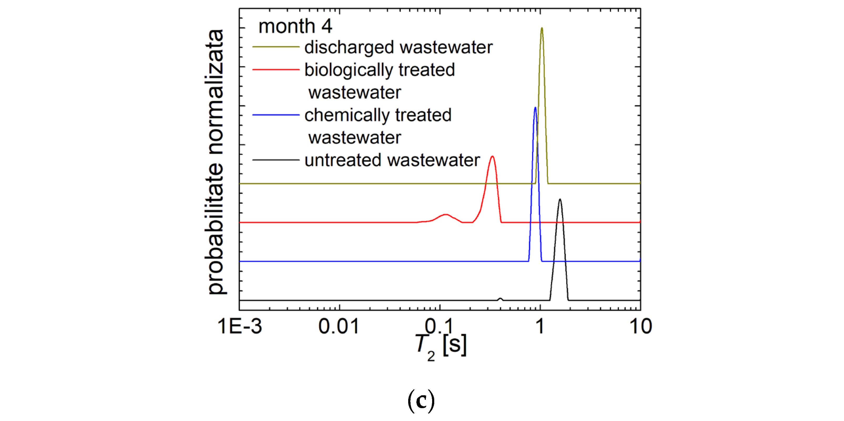
Figure 5.
(a) The most probable T2 values measured from the T2-distribution as maximum of the main peak for all wastewater samples (untreated, chemically and biologically treated and discharged wastewater) and sludge collected from a slaughterhouse in months 1 to 4; (b) The averaged over all months of measurement of the most probable T2 values presented in (a).
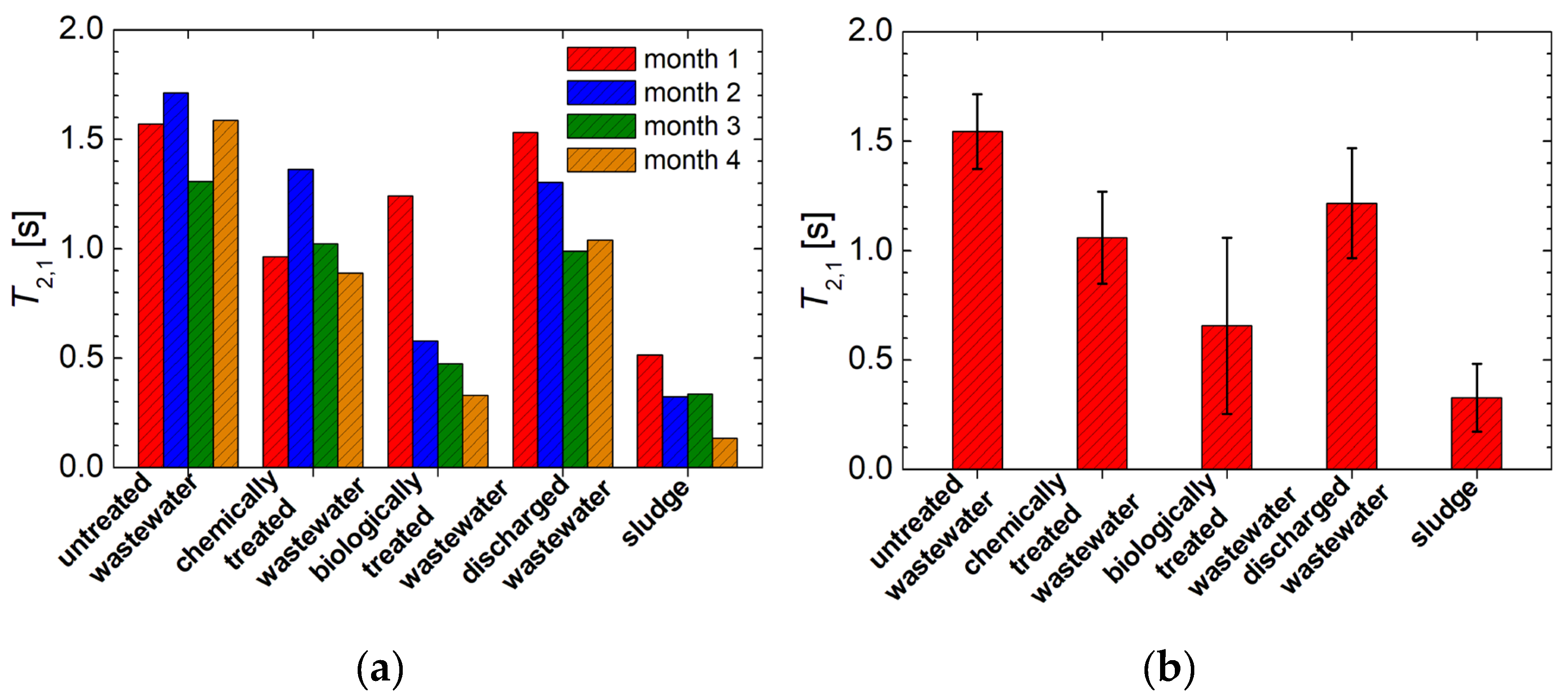
Since the discharged wastewater presents only one peak, identified as the main peak located at the largest T2-values, only the most probable values measured for this peak (here forth named T2,1), associated with water containing dissolved solids, are comparatively presented in Figure 5a. This is due for all four types of wastewater and sludge collected from the chicken slaughterhouse in all four months of monitoring. Relatively large variations are observed for this NMR parameter, especially in samples of biologically treated wastewater and sludge. The normalized T2-distributions of the last one are presented in Figure SI 2 from Supplementary Information. The average values and the standard deviations calculated for those four months of observations are presented in Figure 5b). The largest value of average T2,1 was calculated for the untreated wastewater (~1.54 s), indicating a small amount of dissolved solids in this samples. The relatively small standard deviation values indicate a certain consistency and homogeneity of these samples. The average value of T2,1 calculated for the discharged wastewater (~1.22 s) has a relative large standard deviation compared to the untreated wastewater samples. The larger variability presented by these samples can indicate the degree of the wastewater treatment efficiency. The average T2,1 value for the chemically treated wastewater (~1.06 s) is calculated with a comparable relative measurement error. Though, considering the large overlaps of error bars domains observed for discharged and chemically treated wastewater, one can say that this parameter cannot differentiate those two types of wastewater. Among the wastewater samples, the biologically treated wastewater showed the smallest T2,1 value (~0.66 s) and the largest standard deviations. This clearly indicates the presence of large amounts of dissolved solids in wastewater during the biological treatment stage. As expected, the smallest averaged T2,1 value was calculated for the sludge (~0.33 s). For these samples the relatively large standard deviation values indicate their large variety. Since the untreated wastewater have the average T2,1 value larger than that calculated for discharged wastewater, and to the fact that the average value of T2,1 calculated for chemically treated wastewater is, within the experimental error limit, comparable with that for the discharged wastewater, this parameter (T2,1) alone is not a good indicator of water quality. Therefore other parameters have to be considered, such as the 1H NMR self-diffusion coefficient.
3.2. 1H NMR Diffusometry of Wastewater and Sludge from Chicken Slaughterhouse
The 1H NMR self-diffusion coefficient is a sensitive NMR parameter that can well describe the properties of fluids located in pores, capillaries or in every case in which dissolved particles can influence the fluid molecules mobility, as in our case. Figure 6a) shows (on a logarithmic horizontal scale) the PGSE decays measured for all four types of slaughterhouse wastewater and sludge. As expected, the decay measured for sludge is characterized by the smallest diffusion (due to the strongest limitation of water molecules mobility given by their interaction with large amounts of pollutants) observed as the slowest decaying curve. Such curves are hard to be interpreted quantitatively; therefore a Laplace-like analysis is performed using the kernel presented in eq. (3). The normalized D-distribution functions resulted from this analysis are presented in Figure 6b. The domain of D-distributions had to be extended, compared to the normal domain for the self-diffusion coefficient [49]. This extension becames reasonable by considering, as in the case of relaxation data (see Figure 2b), the split of D-distributions in two: i) the first one corresponding to the self-diffusion of bulk water in the samples (see the blue background in Figure 6b) ranging for our samples from 10-9 m2/s up to (an arbitrary) 10-8 m2/s and ii) the second one associated to water molecules attached to solid residues and transported by flotation and sedimentation, having therefore a larger apparent diffusion coefficient in the range of 10-8 m2/s up to 10-6 m2/s. In this case, the limit of separation between the real self-diffusion coefficient and the apparent diffusion coefficient, describing a flow rather than a self-diffusion process, was chosen in a convenient way between those two domains.
All samples present the largest amount of water as bulk water characterized by the largest peak in the self-diffusion coefficient distribution (Figure 6b). For the first month of monitoring, the wastewater samples (untreated, chemically and biologically treated and discharged wastewaters) presented three peaks, the largest one, as mentioned, in the domain of self-diffusion and two of them in the domain of transported water. It is natural to assume that the largest transport coefficient should be associated with water characterized by a large velocity, therefore a large mobility, specific to small particles that the water is attached to. Contrary, if the water molecules are attached to large particles, the mobility of this water-particle system is small. Therefore, the mobility of attached water is small and it is observed as a small apparent diffusion coefficient. The untreated wastewater leads to a broad peak centered at 2.76 × 10⁻⁹ m2/s. This becames narrow as a result of the purification process that reduces the samples heterogeneity. A narrow peak was also measured for the sludge sample. The most probable self-diffusion coefficient (the peak maximum) increases from 2.76 × 10⁻⁹ m2/s measured for untreated samples of wastewater to 2.76 × 10⁻⁹ m2/s to 2.98 × 10⁻⁹ m2/s for discharged wastewater, indicating an increased mobility (or reduced restrictions). A large value is obtained for chemically treated wastewater (3.03 × 10⁻⁹ m2/s). The lowest most probable self-diffusion coefficient was measured for sludge (2.31 × 10⁻⁹ m2/s). This is normal since this sample contains the largest amount of residues. For the first month of monitoring the D-distributions for sludge present no peaks in the domain of transported water. This is not due to the fact that there are no residues, but on the contrary, it may be due to the fact that the amount of residue is so large that the mobility of water molecules, due to the sedimentation or flotation processes, is strongly reduced. For months of monitoring two to four the D-distributions measured for sludge samples presented similar peaks in the water transport domain (see Figure SI 3 from supplementary information).
Figure 6.
(a) The normalized PGSE decays recorded for the slaughterhouse wastewater (untreated—black square, chemically treated—blue up triangle, biologically treated—red circle and discharged wastewater—dark yellow lower triangle) and sludge collected in month 1; (b) The normalized D-distributions of the PGSE decay curves presented in (a).
Two broad peaks with small amplitude are observed for all the wastewater samples in the transported water domain (Figure 6b—the yellow background). In all cases the integral area under the peaks corresponding to water molecules attached to small particles (the larger D-values, often of the order of hundreds of 10-9 m2/s) is larger than the integral area of peaks corresponding to water molecules attached to large particles (the small D-values, often of the order of tens of 10-9 m2/s). This indicates the presence of larger amounts of small particles in the slaughterhouse wastewater. The largest amount of such small particles was found in untreated wastewater, as expected. The measurement of self-diffusion coefficient distributions for the discharged wastewater (Figure 6b) revealed peaks in the domain of transported water. This was a surprise, given that for the relaxation times T2-distributions the discharged wastewater generated a single peak (see Figure 2b and Figure 4). The presence of several peaks in the D-distributions measured for discharged wastewater associated with water attached to mobile particles indicates that the 1H NMR measurement of the self-diffusion coefficient is a sensitive method than the 1H NMR relaxometry. The area under these peaks indicates the presence of a small amount of such particles in the discharged wastewater. This probably has the same (or appropriate) relaxation time T2 as the bulk water, therefore cannot be distinguished by 1H NMR relaxometry method. The peaks measured in the transported water domain are broad; indicating a large heterogeneity of samples, here translated in a large distribution of particles dimensions. Moreover, the presence of two resolved peaks (instead of just one really broad peak) suggests the presence of at least two types of particles with different origins.
The normalized self-diffusion D-distributions measured for all chicken slaughterhouse wastewater samples collected in months two, three and four of monitoring are presented in Figure 7. Generally, the characteristics previously described for month one of monitoring are also valid for these samples. One can remark: i) the similarly small deviation of the most probable self-diffusion coefficient (measured at maximum of peaks from D-distributions) that from here-on will be labeled with D1; ii) the large amount of water attached to small particles especially for untreated wastewater, chemically treated wastewater and discharged wastewater; iii) a comparable or small amount of water attached to small particles (D of the order of hundreds of 10-9 m2/s—from now-on labeled as D3) than those attached to large particles (D of the order of tens of 10-9 m2/s—from now-on labeled as D2).
The measurement parameters (magnetic field gradients and delays in the PGSE pulse sequence—see Figure SI 1b from supplementary information) are calibrated for a good measurement of the bulk water self-diffusion coefficient. For our samples this parameter (D1) is measured with the largest precision (affecting the full decay curve—see Figure 6a) compared with the apparent diffusion coefficient D2 and D3. The latter two are measured with a small precision since, being with one or two order of measurement larger (than D1) can affect only fewer points at the beginning of the decay PGSE curve.
Figure 7.
The normalized D-distributions recorded for the slaughterhouse wastewater: untreated (black), chemically treated (blue), biologically treated (red) and discharged wastewater (dark yellow) collected in (a) month 2; (b) month 3; (c) month 4 of monitoring.
Figure 7.
The normalized D-distributions recorded for the slaughterhouse wastewater: untreated (black), chemically treated (blue), biologically treated (red) and discharged wastewater (dark yellow) collected in (a) month 2; (b) month 3; (c) month 4 of monitoring.

For a quantitative analysis of purification process via self-diffusion, only the D1 diffusion coefficient will be considered. All D1 values measured for all four types of wastewater samples and sludge for all four months of monitoring are comparatively presented in Figure 8a. With some exceptions (month two for untreated wastewater and biologically treated wastewater, and month one for chemically treated wastewater, discharged wastewater and sludge), the measured value of the most probable self-diffusion coefficient D1 are similar for the rest of three months. The average of all four months and the measurement errors are presented in Figure 8b. Within the experimental error limit, one can observe that the D1 parameter can be used to differentiate between the types of wastewater. An overlap only exists between the chemically treated wastewater and the discharged wastewater. The smallest D1 value (and the largest error) was measured for sludge, and the largest ones were measured for chemically treated wastewater and for discharged wastewater. In conclusion, the large value measured of the self-diffusion coefficient D1 for discharged wastewater indicates a small restriction of the water molecules mobility and therefore a good efficiency of the wastewater purification applied in the chicken slaughterhouse.
3.3. VIS-NearIR Spectroscopy
Both 1H NMR relaxometry and diffusometry, as previously discussed, show that even in the discharged wastewater from chicken slaughterhouse, there is a variety of particles visible or invisible to the naked eye. These particles will affect (by absorption) the visible light that eventually passes through wastewater. The classical method largely used to quantify the amount of such particles is by determining its turbidity [3]. This is a global parameter, giving a single value for a specific sample. We propose to replace the turbidity measurement by acquiring a VIS-nearIR spectrum.
Figure 9.
The VIS-nearIR absorbance measured for the chicken slaughterhouse wastewater and 1 ml of sludge residues distilled in 20 ml of distilled water collected in month 1 of monitoring.
Figure 9.
The VIS-nearIR absorbance measured for the chicken slaughterhouse wastewater and 1 ml of sludge residues distilled in 20 ml of distilled water collected in month 1 of monitoring.
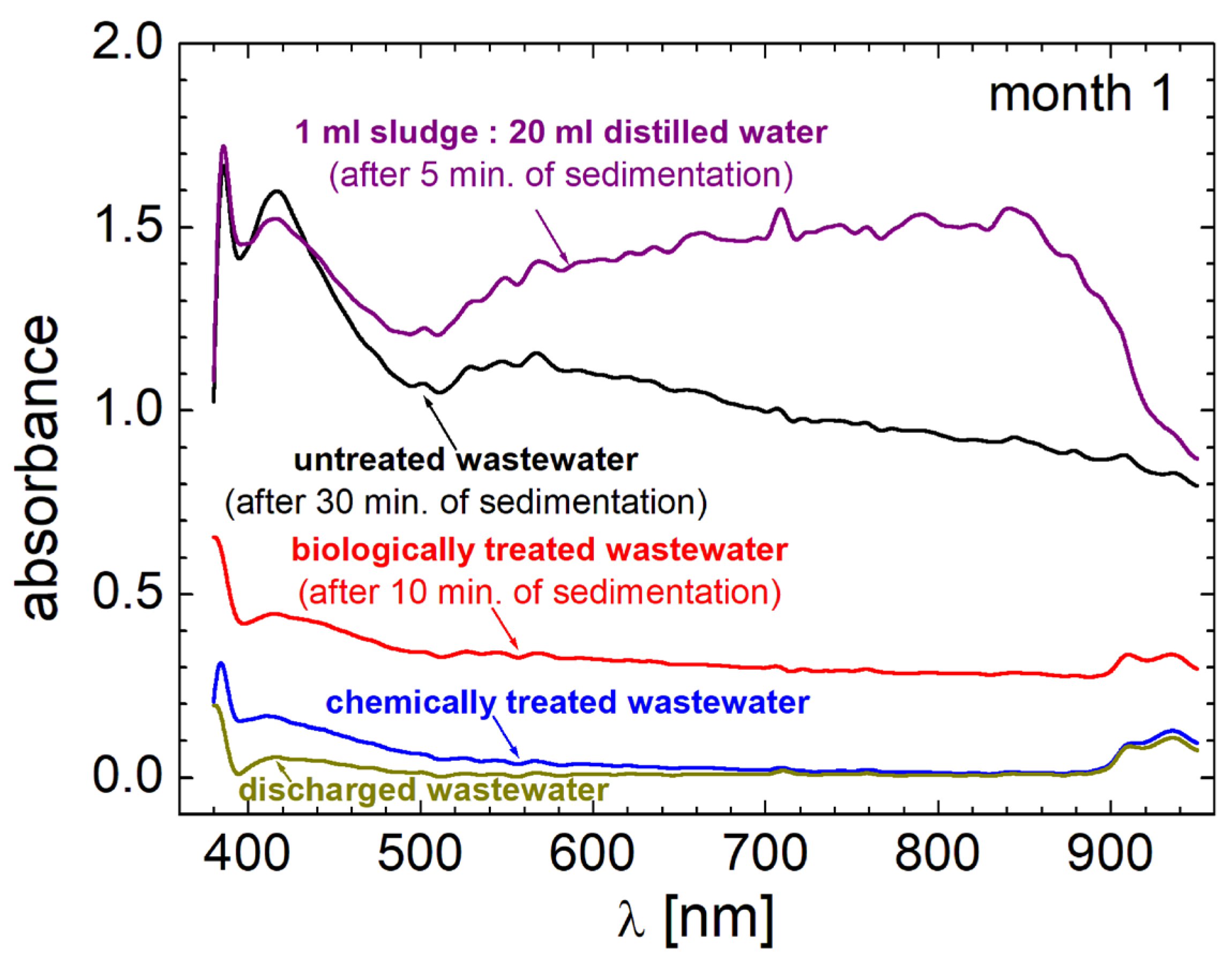
An example of such VIS-nearIR spectra recorded for untreated wastewater (after 30 minutes of sedimentation), chemically treated wastewater, biologically treated wastewater (after 10 minutes of sedimentation), discharged wastewater and sludge (1 ml of sludge distilled in 20 ml of distilled water and then measured after 5 minutes of sedimentation) for samples collected in month one of monitoring, are presented in Figure 9. The array sensor of Pasco VIS-nearIR spectrometer allowed us to record the spectra in seconds, therefore, the sedimentation and/or flotation process will not affect the spectral amplitude function of wavelength. This was a problem when a similar measurement was attempted using a step-by-step UV-VIS spectrometer, when the measurement is performed by gradually changing the wavelength, and then the measurement lasted for several minutes. All wastewater and sludge solution present a large absorption in violet light (possible extended in the ultraviolet domain). One can also observe a certain absorption at the wavelength of ~420 nm, then the discharged wastewater, chemically and biologically treated wastewater present a certain decay of the absorbance with the increasing the light wavelength. For these samples, one can observe a certain absorption doublet in the infrared domain at wavelengths larger than 900 nm. For the untreated wastewater, one can observe an additional relative maximum of absorption at λ ~ 560 nm at a so called Chartreuse color between green and yellow. Similar features are observed in sludge solution and in untreated wastewater, except for the fact that the absorbance through the sludge solution is not decaying for wavelengths larger than 560 nm up to ~ 840 nm that belong to the near infrared domain.
An extensive analysis can be performed of the light absorption function of wavelength correlated with the particles sizes and types of pollutants. Such analysis is beyond our scope, therefore will not be discussed here. Nevertheless, it is important to observe that the VIS-nearIR spectroscopy is sensitive to the degree of pollution of wastewater, presenting the largest absorbance for the sludge (even if it was diluted 1:20 in distillated water) and then for the untreated wastewater. Next, less absorbance was measured for the biologically treated wastewater (since it was collected before sedimentation). A small absorbance was measured for chemically treated wastewater and the cleanest wastewater was found the discharged wastewater. Among of all our methods, it is the VIS-nearIR spectroscopy that more accurately reveals the purification process. Unfortunately, this method also can be affected by large errors, as moving particles enter (by sedimentation and/or flotation) between the LED light source and detector, and by data sampling. Going back to a single parameter aimed to characterize the VIS-nearIR spectra, we found the total absorbance, i.e. the integral area under each spectrum. This parameter (in arbitrary units) is presented in Figure 10 a) for all wastewater samples and sludge and for all four months of monitoring. Large variations can be observed in untreated wastewater, biologically treated wastewater and sludge. The statistical average of the total absorbance and the measurement errors are presented in Figure 10 b). Large error bars are observed for the samples enumerated before. One can remark the small values for the averaged total absorbance measured in chemically treated wastewater and in discharged wastewater. This is a new proof that the wastewater purification process applied at the chicken slaughterhouse is efficient. We also performed a correlation/calibration measurement for some milky-like samples over a wide range of turbidity degrees, and we found that the total absorbance measured from VIS-nearIR spectra can replace the turbidity measurement with a proper calibration, since the dependence in the domain 0–500 ntu is linear. Over this limit of 500 ntu, there is a non-linear relationship. The resulted calibration curve is given in Figure SI 4 in Supplementary Information. Finally, the large variation of data in VIS-nearIR spectra can be reduced by multiple sampling and an appropriate statistical average.
3.4. The pH Measurements
A largely used parameter for water testing is its pH. The wastewater pH values for all samples (untreated, chemically and biologically treated, discharged wastewater and sludge solution) collected in all four months were measured and are shown in Figure 11 a). Large variations can be observed among samples collected in different months. One can remark a minimum value for pH of ~5.1 and a maxim value of ~8.4, both being measured for samples collected in month one of monitoring. Interesting results are obtained for the average values calculated for all four months of monitoring. These values are presented in Figure 11 b) together with the statistical measurement errors. The average pH values can be found between ~6.5 for discharged wastewater and ~6.8 for chemically and biologically treated wastewater. Nevertheless, within the experimental error limits (the maximum pH error was calculated for chemically treated wastewater at approximately ± 1) one cannot distinguish the samples by measuring the pH parameter. Even the sludge solution (the sludge pH was measured for the solution prepared for the VIS-nearIR spectroscopy) has the pH between the same limits. One also observes that the pH was a controlled parameter for the chemically treated wastewater, its value measured for the wastewater automatically opens the valves of the coagulant, NaOH and liquid polymer tanks.
3.5. Electric Conductivity Measurements
The dissolved and undissolved pollutants will change the electric conductivity (EC) of slaughterhouse wastewater. Figure 12a) presents the measured values for all types of wastewater and sludge (in solution as was prepared for VIS-nearIR spectroscopy) collected in all four months of monitoring. As in the case of pH measurements, large differences of the electric conductivity values can be observed comparing samples collected in different months. The average values together with the standard deviations are presented in Figure 12b). In general, for the same type of dissolved particles, a large value measured for the electric conductivity implies a large concentration of pollutants. The average values of electric conductivity σ, show a decay from untreated wastewater to chemically and biologically treated wastewater. This showed similar values of σ, while the discharged wastewater is characterized by the smallest σ value. Contrary to pH, in the case of electric conductivity, the value measured for sludge is substantially larger compared to the values measured for all the types of wastewater. Taking a look to the magnitude of error bars, the first idea is that the electric conductivity, despite of the average values, cannot be used to discriminate between different kinds of wastewater. On the contrary, as we will see in subchapter dedicated to statistical analysis in principal components, not only that the electric conductivity can be successfully used in differentiation between all four types of wastewater, but together with total dissolved solids it proves to be an important parameter.
3.6. Total Dissolved Solids Measurements
A total dissolved solid (TDS) is a global parameter that, as in the case of electric conductivity, is usually applied for the characterization of the pollution degree in wastewaters, in particular for those collected from chicken slaughterhouses. In fact, often these two parameters are well correlated. This is a feature that was also observed for our samples. In Figure 13 a) are presented the measurement of TDS values for all the wastewater samples (untreated, chemically and biologically treated and discharged wastewater) and sludge, for all four months of monitoring. With some minor differences, these values look similar to those measured for the electric conductivity (see Figure 12 a) and Figure 13 a)). As in the case of electric conductivity, the TDS values are out of range for samples collected in month one of monitoring for untreated wastewater, biologically treated wastewater and sludge. Contrary to the measurement of EC in the case of TDS for the month four of monitoring the data seems to be in the same range with the rest of values measured for the samples collected before. The average TDS values and the measurement errors are comparatively presented in Figure 13 b). A large value is obtained for the untreated wastewater (~585 ppm). Similar values are obtained for chemically and biologically treated wastewater (427.75 ppm and 426.5 ppm, respectively). As a result of purification, the discharged wastewater has an averaged value of TDS of ~392.5 ppm. The relative elevated value of TDS measured for the discharged wastewater is in agreement with the 1H NMR diffusometry measurements (Figure 6 b) and Figure 7), VIS-nearIR spectroscopy (Figure 9), and electric conductivity (Figure 10), which all showed that the discharged wastewater is not pure, contrary to the interpretation of 1H NMR relaxometry data (Figure 2 a) and Figure 4). Moreover, it will be shown later than the TDS measurements are important data for the discrimination between different types of wastewater and sludge via statistical analysis of the principal components.
3.7. Principal Component Analysis
The way in which one can analyze variate data types characterized by variables with different measurement units is the statistical multivariate analysis, in particular the analysis of the principal components [55,56]. For our analysis, we implement numerically our own analysis program written in MatLab and we plotted the results using Microsoft Excel. The data were verified using PAST Version 3.25 which stands for PAleontological STatistics software and Origin 2022b (Academic). For the principal component analysis we produced an input data matrix with the most relevant parameters (in number of six) as they are listed in Table 1. As variables, we selected: i) the total absorbance as was measured from VIS-nearIR spectra (see Figure 9); ii) the T2,1 spin-spin relaxation times values measured as the most probable value for the water with dissolved solids (see Figure 2 b) and Figure 4); iii) the self-diffusion coefficient D1 values corresponding to bulk water measured as the most probable coefficient from the maximum of D-distribution (see Figure 6b); iv) the pH (see Figure 11a); v) the electric conductivity, EC (see Figure 12a) and vi) the total dissolved solids (see Figure 13a). These values are listed for all types of wastewater (untreated, chemically treated, biologically treated and discharged wastewater) and sludge which are considered to represent a particular group, and all four months of monitoring are considered as particular variations in each group. In total, the matrix contains six columns (representing the independent parameters) and 20 rows (representing the number of measured data for each parameter). Since the number of independent parameters is smaller than the number of data, then this will give the number of principal components (PC). Therefore, in our case the number of PC was six. The analysis is similar to an eigenvectors/eigenvalues problem. The proportion with the contribution of each component and the cumulative proportion are presented in figure SI 5a from supplementary information. One can see that the first component (PC1) can explain ~48.9 from the variation in experimental data. If the PC2 is also considered, then ~69.3% of the variations can be explained. In order to pass over 90%, PC3 and PC4 must also be considered. The eigenvalues functions of the PC number are presented in figure SI 5 from supplementary information.

Table 1.
The values of relevant parameters (total VIS-nearIR absorbance, the most probable transverse relaxation time T2,1, the self-diffusion coefficient D1, pH, electric conductivity EC and the total dissolved solids TDS) measured for the slaughterhouse wastewater (untreated, chemically treated, biologically treated and discharged) and sludge collected during four months of monitoring.
| wastewater | month | Total VIS-nearIR absorbance |
T2,1 [s] |
D1 [10-9 m2/s] |
pH [–] |
EC [μS/cm] |
TDS [ppm] |
|---|---|---|---|---|---|---|---|
| untreated wastewater | 1 | 1.06* | 1.57 | 2.76 | 5.11 | 478 | 263 |
| 2 | 0.14 | 1.71 | 2.86 | 6.75 | 1596 | 795 | |
| 3 | 1.401* | 1.31 | 2.78 | 7.16 | 1236 | 618 | |
| 4 | 2.13* | 1.59 | 2.81 | 7.17 | 658 | 658 | |
| chemically treated wastewater | 1 | 0.06 | 0.96 | 3.03 | 8.4 | 947 | 470 |
| 2 | 0.04 | 1.36 | 2.88 | 6.03 | 860 | 484 | |
| 3 | 0.05 | 1.02 | 2.90 | 6.35 | 740 | 374 | |
| 4 | 0.02 | 0.89 | 2.95 | 6.53 | 383 | 383 | |
| biologically treated wastewater | 1 | 0.33** | 1.24 | 2.68 | 7.15 | 1182 | 597 |
| 2 | 0.14** | 0.58 | 2.81 | 7.29 | 822 | 412 | |
| 3 | 2.99** | 0.47 | 2.68 | 6.25 | 686 | 344 | |
| 4 | 0.04** | 0.33 | 2.67 | 6.66 | 353 | 353 | |
| discharged wastewater | 1 | 0.02 | 1.53 | 2.98 | 7.52 | 860 | 433 |
| 2 | 0.02 | 1.30 | 2.86 | 5.84 | 429 | 429 | |
| 3 | 0.03 | 0.99 | 2.91 | 6.56 | 704 | 352 | |
| 4 | 0.002 | 1.04 | 2.88 | 6.61 | 356 | 356 | |
| Sludge | 1 | 1.39*** | 0.52 | 2.31 | 7.23 | 2880 | 1662 |
| 2 | 0.33*** | 0.32 | 2.62 | 6.92 | 2070 | 1045 | |
| 3 | 0.43*** | 0.34 | 2.66 | 6.13 | 1668 | 826 | |
| 4 | 0.32*** | 0.14 | 2.60 | 6.94 | 963 | 963 |
* Measured after 30 minutes of sedimentation; ** Measured after 10 minutes of sedimentation; *** Measured after 5 minutes of sedimentation; In all cases the measurement errors are smaller than 5%.
4. Discussion
Principal component analysis (PCA) is a powerful tool to assess the statistical behavior of measured data, allowing to discriminate different parts of a statistical system, to find correlations between different types of parameters and if it is the case, to observe an evolution process. The main result of the application of PCA analysis on our slaughterhouse wastewater measurements is presented in Figure 14 as a plot of PC2 (second principal component) in correspondence with PC1 (the first principal component). The data must be analyzed in close relationship with the results listed in Table 2. Here, the contributions of each parameter (the total absorbance of VIS-nearIR spectra, T2,1 spin-spin relaxation time, the self-diffusion coefficient D1, pH, EC and TDS) to the principal components PC1 to PC6 are given. To assess the importance of a specific parameter to each principal component, only the magnitudes of listed values must be considered. The sign of listed values will contribute to the displacement of data presented in Figure 14 and will led to the separation between different types (groups) of samples. The first principal component PC1 is characterized by the largest separation of data and the displacement (variation) decays with the increase of principal component number, PC6 having the smallest displacement. A PCA statistical analysis is considered to be successful (the number and the type of chosen parameters is relevant, the data are correlated, etc.) if the data presented in a two- (as in the case of plot in Figure 14) or a multi-dimensional space presents a cluster behavior. This means that the points representing the data from the same group are found together and as far away as possible from other groups. Analyzing real data, affected by many types of errors, one can find overlapping regions between different groups and often there will be point(s) that are missed (located away) from a designated group.
In Figure 14 the group of four points (month one to four of monitoring) corresponding to untreated wastewater is shown with blue diamond. For months 2, 3 and 4 these points are located to the center of figure having the smallest PC1 and PC2 values. The point corresponding to month one of monitoring for untreated wastewater is located at a large negative PC1 and PC2. Table 2 summarizes the main contributions to PC1: the global parameters TDS (0.933) and EC (0.884), and the specific NMR self-diffusion coefficient D1 (-0.892). A certain contribution can be found from the T2,1 NMR parameter (-0.561). The smallest contribution to PC1 comes from pH (0.25) and total absorbance in VIS and near IR (0.336). Conversely, the main contribution to the second principal component PC2 comes from pH (0.794). Also, with a large contribution can be credited the total VIS-nearIR absorbance (-0.627). To PC2 an insignificant contribution comes from T2,1 (0.054), then comes the TDS (0.165) and EC (0.22). The NMR self-diffusion coefficient D1 will have a relative important contribution (0.343). Therefore, the measurements of pH, EC and TDS performed for samples collected in month one of monitoring are out of range. A similar behavior can be found for biologically treated wastewater (red filled square in Figure 14). Here, the points corresponding to samples collected in months 1, 2 and 4 are grouped and the point corresponding to month 3 is largely displaced in the negative direction of PC2. Therefore, the pH value and the total absorbance in VIS-nearIR measured for this sample are the main responsible with this out of group position. Grouped at negative values of PC1 can be found the points belonging to chemically treated wastewater (shown with filled green triangles) and discharged wastewater (filled yellow square). Especially in PC1, one can observe a good grouping behavior with only a small variation. From the point of view of PC1, the biologically treated wastewater (PC1: from -0.46 to 0.81—without month 3) is the most similar to the untreated wastewater (PC1: from -2.53 to -1.92—without month 1). While the discharged wastewater (PC1: from -2.57 to -2.06) is the most different from untreated wastewater. From the point of view of the purification process this is a very good observation. One can extend this kind of analysis. By taking a look to the cluster of discharged wastewater one can see that the chemically treated wastewater (for months 2, 3 and 4) will have similar properties to those of the discharged wastewater. From the point of view of PC1, the chemically treated wastewater (PC1: from -2.53 to -1.92—without month 1) collected in month 3 of monitoring is cleaner (different from untreated wastewater) than the discharged wastewater collected in months 3, 1 and 4. Although, if the data are well grouped in PC1, the points representing the properties of samples collected in month one of monitoring for chemically treated and discharged wastewater, in PC2 these are away from the group center of gravity. Mostly, the pH measured for these samples (of chemically treated wastewater and discharged wastewater) led to this displacement.
A completely opposed behavior is observed for sludge (blue circles). The group of these samples is localized at positive large values of PC1, well separated even from untreated wastewater. In the second component one observes that the values are distributed around the zero value of PC2. Then, one can conclude that PC1 can be used to successfully separate the wastewater according to is purity. So that the most contaminated sample was the sludge sample, collected in month one of monitoring and the cleanest wastewater was the wastewater sample collected in month two of monitoring. For our wastewater system (also containing the sludge), one can see that the most significant parameters were (in order): i) the total dissolved solids TDS; ii) the self-diffusion coefficient D1; iii) the electric conductivity EC and iv) the transverse relaxation time of dissolved solids T2,1. The most irrelevant parameter was pH. Nevertheless, pH and the total absorbance in VIS-nearIR are important parameters capable to identify samples (in PC2) from the same group with properties away from the average expectation.
Figure 15.
The double linear correlation between electric conductivity (EC) and totally dissolved solids (TDS) for the wastewater and sludge.
Figure 15.
The double linear correlation between electric conductivity (EC) and totally dissolved solids (TDS) for the wastewater and sludge.
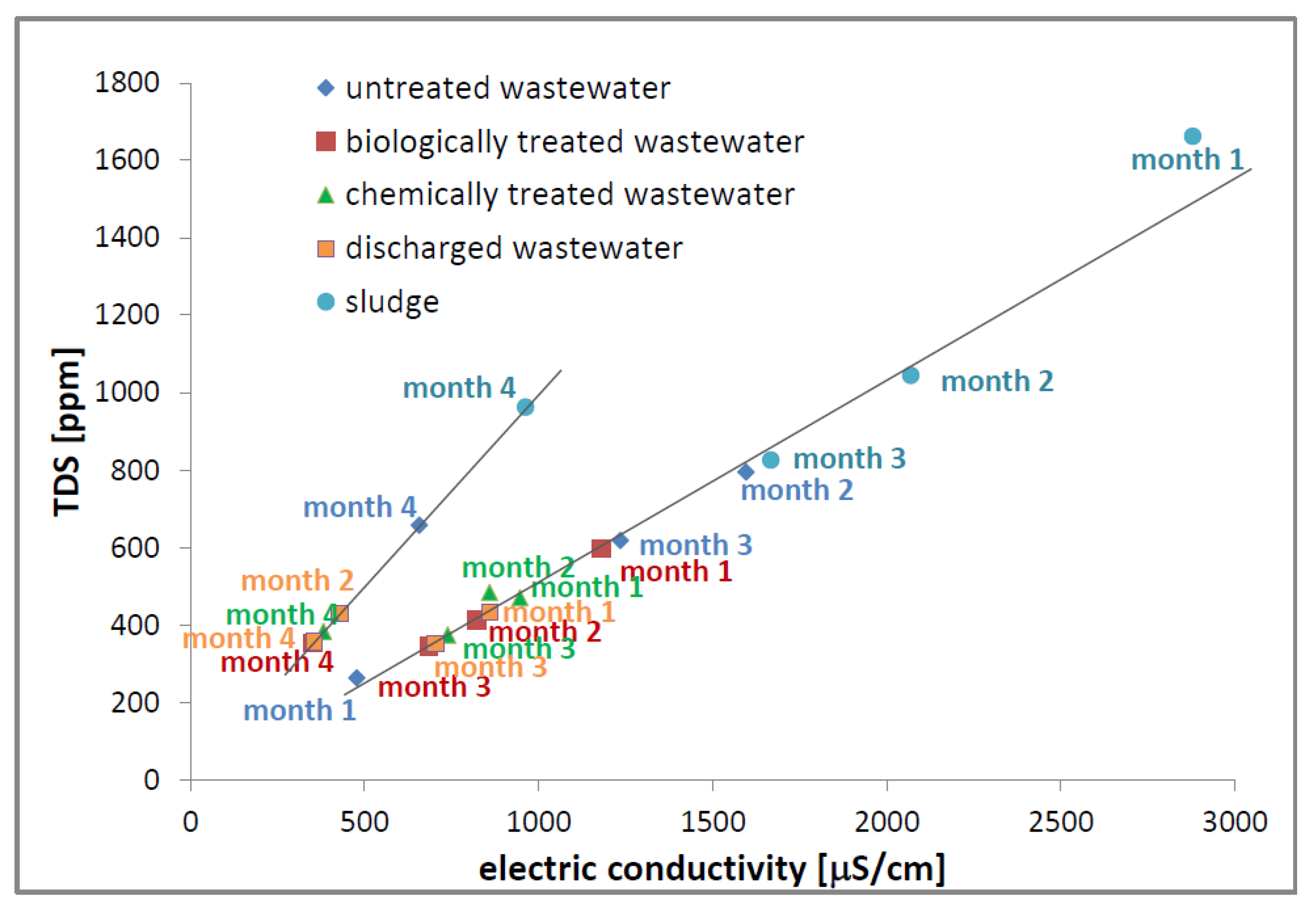
Another important result of our PCA assay is the degree of correlation between all parameters considered in pairs. In this case of wastewater collected from a chicken slaughterhouse the most correlated parameters were found to be the electric conductivity, EC and the total dissolved solids, TDS. This is not a surprise since, the physical support of the electric conductivity is given by dissolved solids; being known that distilled water presents a poor electric conductivity. Considering the elements of a covariance matrix C (using the MatLab numeric program, but not from PAST software), that the eigenvectors and eigenvalues problem was solved for; one can see the large value for the elements (there are two symmetrical around a main diagonal that has values of 1, meaning that each parameter is perfectly correlated with itself) correspond to the EC and TDS parameters. Though, the values are not as large as expected. To understand that, in Figure 15 the TDS is plotted as a function of EC. Now the correlation coefficient can be better understood. The first observation is that indeed the TDS is well correlated to the EC parameter, but in our case, for all samples collected from the chicken slaughterhouse in four months of monitoring, there are two linear dependences rather than a single one. With one exception, one can see that the data (TDS and EC) measured for months 1, 2 and 3 of monitoring for untreated, chemically and biologically treated wastewater; discharged wastewater and sludge are in a very good linear correlation. While, the data collected in the four month of monitoring are arranged on a second linear dependence. Usually, such double linear correlations can be explained: i) by a change in the treatment process (to include different types of particles with another electrical behavior); ii) by a change of dissolved pollutants, or iii) by both causes. In our case the most probable cause is the fact that the wastewater samples collected in month four of monitoring of wastewater were used in the processing of different kind of chickens (with a different origin, size, age, etc). An interesting observation is the fact that the point corresponding to the discharged wastewater collected in month 2 is placed on the short dependency belonging to month 4.
In the last time, artificial intelligence is used in more and more fields, from entering in parking place to cancer prediction [56]. We developed a dedicated program written in JavaScript (JS) that used an online library named ML5 [58], to easily build an Artificial Neural Network (ANN). This is used to predict the probability that a new measurement of all parameters analyzed by PCA to be classified as untreated wastewater, chemically or biologically wastewater, discharged wastewater, or sludge (see Figure 16). We simulated the incidence of such analysis in every element of a 100 × 100 matrix associated to the 2D plot of the main PCA analysis (see Figure 14). Prior to that, the JS loaded the 5 × 4 = 20 values of PC1 and PC2 coordinated together with the label associated with our five types of samples (four wastewater and sludge). The ANN was trained for 10000 epochs with a learning rate of 10% and the trained model was saved to be loaded anytime that is needed (without any new training, which is a time consuming procedure). Once the trained model is loaded, it can be used to generate prediction related to the probability that in a chosen position (in the main analysis 2D space) resulted from a PCA analysis of a new element the sample to be associated one of the trained labels (i.e. untreated wastewater, chemically treated wastewater, biologically treated wastewater, evacuated wastewater or sludge). The generated prediction maps, which simplify even more the PCA analysis, are presented in Figure 16. Thus, Figure 16a presents the predicted probability (measured from 0 to 1, where 1 represents 100%) for untreated wastewater. One can observe that the maximum probability is obtained for PC1 and PC2 negative (see also Figure 14) especially due to the sample collected in month 1. A relative maximum (around 50%) is obtained for PC1 and PC2 values closed to zero especially due to the samples collected in months 2 and 3. The PCA analysis of chemically treated wastewater can be found with high probability (>70%) if PC1 is between -3 to -1 and PC2 larger than 1 (see Figure 16c). A high probability to associate, in the PCA analysis, the measured result with biologically treated wastewater is to have PCA between -1 and 0 and PC2 to have large positive or negative values (see Figure 16c). From Figure 16c one can see that a smaller PC1 value (almost independent on PC2 value) it is associated to the discharged wastewater (see Figure 16d). Values of PC1 larger than zero can be associated with a high probability to a measured sludge (see Figure 16e). The prediction maps can offer enhanced representation of sample classification related to the PCA analysis.
Such prediction maps were produced and discussed in ref. [54], where Dragan et al. classify data measured by NMR and FT-IR to various types of colorectal cancer. But, according to our knowledge, this is the first time when such predictions are used to classify the wastewater and sludge resulted from slaughterhouse activity.
5. Conclusions
This is one of the most complex studies related to the characterization of wastewater collected from slaughterhouses. This complexity is based on both, the large variety of measured parameters using modern and classical methods, but also on the many levels of analysis which starts with raw measurement, then continues with the ILT analysis of measured data and primary classification. Then continues with statistical analysis in principal components which finally is used to train an artificial neural network to predict and classify new measurements. For that, a series of wastewater samples collected during four months of monitoring from a chicken slaughterhouse wastewater treatment plant over different stages in the purification process (starting with the untreated wastewater, then from chemically treated basin, from SBR biologically treatment basin, ending to the discharged wastewater and adding samples from sludge) were analyzed using advanced spectroscopic methods like the low field 1H NMR relaxometry and diffusometry and VIS-nearIR spectroscopy and by using the classical methods of determining the pH, the electric conductivity and the totally dissolved solids. It was demonstrated the advantage of using the model-free low field 1H NMR relaxometry and diffusometry combined with the Laplace-like analysis compared to the classical ones, which provides a global single value for the entire sample, to a more realistic characterization of wastewater dynamic components. This analysis shown that the distributions of 1H NMR transverse relaxation times T2 present two distinct domains. The first one is characterizing the water with dissolved solids and the second one is characterizing the water with undissolved solids. Moreover, according to the 1H NMR relaxometry measurements, the untreated wastewater and the biologically treated wastewater present the largest number of components. While, the chemically treated wastewater and discharged wastewater presents only one component of water with dissolved solids. The most probable relaxation time T2,1 characterizing the water with dissolved solids was the selected parameter for a statistical analysis. Additionally, it was shown that the distribution of 1H NMR self-diffusion coefficient, D also presents two domains. These are the self-diffusion in bulk water and the transported water attached to solid residues and flowing by flotation and sedimentation. The 1H NMR diffusometry measurements proved that even the discharged wastewater is not completely clean of undissolved solids. The most probable self-diffusion coefficient D1 was another selected parameter for the statistical analysis. We also show that, via a calibration curve, the turbidity measurement can be replaced by a VIS-nearIR spectrum of which total absorbance depends linearly on turbidity in the range of 0 to 500 ntu. Moreover, even for larger values a calibration curve can exist. The total absorbance was the third selected parameter for the PCA statistical analysis. To assess the contribution of each parameter to the evaluation process of the efficiency of purification treatment performed by a chicken slaughterhouse, a statistical analysis in principal components was performed. For that, the list of parameters was completed with pH, electric conductivity (EC) and totally dissolved solids (TDS). It was found that the most important parameters, having the largest influence on PC1 (first principal component) were (in order), TDS, D1 and EC. PC1, being the components along which the dispersion was maximum, was able to separate the most polluted sample at extreme positive values and the most purified wastewater at extreme negative values. PC2 is most influenced by the samples’ pH. The presented statistic in PCA is not unique. Other parameters can be added (or excluded) from the PCA attempt. In our case, for the selected parameters, the groups were well differentiated in less polluted wastewater (discharged wastewater and chemically treated wastewater) heavily polluted wastewater (untreated wastewater and biologically treated wastewater) and sludge. It was shown how the PCA analysis can be further improved if is used to train an ANN to predict and classify a new measurement to one of the studied category of wastewater or sludge. Finally, from the analysis of the distributions of transverse relaxation times T2 and diffusion coefficient D, the VIS-nearIR spectra and EC and TDS measured parameters, one can conclude that the purification process performed by the chicken slaughterhouse is efficient.
Supplementary Materials
The following supporting information can be downloaded at the website of this paper posted on Preprints.org. Figure SI 1: The CPMG and PGSE pulse sequences; Figure SI 2: The T2-distributions measured for sludge; Figure SI 3: The self-diffusion coefficient D distributions measured for sludge; Figure SI 4: The relationship between the total absorbance in the VIS-NearIR spectra and turbidity and Figure SI 5: The proportions and eigenvalues resulted from PCA applied on the measured parameters of poultry slaughterhouse wastewater.
Author Contributions
R.C. collected the samples, conceived, designed and performed the experiments, primary and secondary data analysis, statistical analysis, revised and proofread the paper; R.F. conceived and designed the experiments, wrote the numerical software for advanced data analysis, wrote and revised the paper.
Funding
This research received no external funding.
Acknowledgments
The authors would like to thank to S.C. AGROPROD CRASNA Cooperativa Agricolă S.R.L., Satu-Mare, Romania in particular to Daniel Pereș and Petru Crainic for providing the chicken slaughterhouse wastewater samples and relevant information about the wastewater treatment. The authors thanks also to Assoc. Prof. Dr. Simona Nicoara for suggestions of English corrections.
Conflicts of Interest
The authors declare no conflict of interest.
References
- Paulista, L.O.; Presumido, P.H.; Peruço Theodoro, J.D.; Novaes Pinheiro, A.L. Efficiency analysis of the electrocoagulation and electroflotation treatment of poultry slaughterhouse wastewater using aluminum and graphite anodes. Environ. Sci. Poll. Res. 2018, 25, 19790–19800. [Google Scholar] [CrossRef] [PubMed]
- Aceves-Lara, C.-A.; Latrille, E.; Conte, T.; Steye, J.-P. Online estimation of VFA, alkalinity and bicarbonateconcentrations by electrical conductivity measurementduring anaerobic fermentation. Water Sci. Technol. 2012, 65, 1281–1289. [Google Scholar] [CrossRef]
- Yusoff, M.S.; Azwan, A.M.; Zamri, M.F.M.A.; Aziz, H.A. Removal of colour, turbidity, oil and grease for slaughterhouse wastewater using electrocoagulation method. AIP Conf. Proc. 2017, 1892, 040012-1–040012-7. [Google Scholar]
- Khanna, V.K. pH measurement of dirty water sources by ISFET: addressing practical problems. Sensor Review 2007, 27, 233–238. [Google Scholar] [CrossRef]
- Modla, M. The easy guide to pH measurement. Meas. Control 2004, 37, 204–206. [Google Scholar] [CrossRef]
- Ferraz, F.M.; Yuan, Q. Nitrite interference with soluble COD measurements from aerobically treated wastewater. Water Environ. Res. 2017, 89, 549–554. [Google Scholar] [CrossRef]
- APHA. Standard Methods for the Examination of Water and Wastewater, 22nd ed.; American Public Health Association: Washington, DC, USA, 2012. [Google Scholar]
- Boughou, N.; Majdy, I.; Cherkaoui, E.; Khamar, M.; Nounah, A. Physico-chemical characterization of wastewater from slaughterhouse: Case of rabat in Morocco. ARPN J. Agric. Biol. Sci. 2018, 13, 19–24. [Google Scholar]
- Crainic, R.; Drăgan, L.R.; Fechete, R. 1H NMR relaxometry and ATR-FT-IR spectrosopy used for the assesment of wastewater treatment in slaughterhouse. Studia UBB Phys. 2018, 63, 49–60. [Google Scholar] [CrossRef]
- Seif, H.; Moursy, A. Treatment of slaughterhouse wastes. In Sicth international water conference; IWTC: Alexandria, Egypt, 2001; pp. 270–271. [Google Scholar]
- Alayu, E.; Yirgu, Z. Advanced technologies for the treatment of wastewaters from agro-processing industries and cogeneration of by-products: a case of slaughterhouse, dairy and beverage industries. Int. J. Environ. Sci. Technol. 2018, 15, 1581–1596. [Google Scholar] [CrossRef]
- López-Maldonado, E.A.; Oropeza-Guzman, M.T.; Jurado-Baizaval, J.L.; Ochoa-Terán, A. Coagulation–flocculation mechanisms in wastewater treatment plants through zeta potential measurements. J. Hazard. Mat. 2014, 279, 1–10. [Google Scholar] [CrossRef]
- Mehmood, K.; Rehman, S.K.U.; Wang, J.; Farooq, F.; Mahmood, Q.; Jadoon, A.M.; Javed, M.F.; Ahmad, I. Treatment of Pulp and Paper Industrial Euent Using Physicochemical Process for Recycling. Water 2019, 11, 2393. [Google Scholar] [CrossRef]
- Zamani, H.; Golestani, H.A.; Mousavi, S.M.; Zhiani, R.; Hosseini, M.S. Slaughterhouse wastewater treatment using biological anaerobic and coagulation-flocculation hybrid process. Desal. Wat. Treat. 2019, 155, 64–71. [Google Scholar] [CrossRef]
- Lazaridis, N.K.; Matis, K.A.; Webb, M. Flotation of metal-loaded clayanion exchangers. Part I: the case of chromate. Chemosphere 2001, 42, 373–378. [Google Scholar] [CrossRef] [PubMed]
- Doyle, F.M.; Liu, Z.D. The effect of triethylenetraamine (trien) on the ion flotation of Cu2+ and Ni2+. J. Colloid Interface Sci. 2003, 258, 396–403. [Google Scholar] [CrossRef] [PubMed]
- Khandegar, V.; Saroha, A.K. Electrocoagulation for the treatment of textile industry effluent e A review. J. Env. Management 2013, 128, 949–963. [Google Scholar] [CrossRef] [PubMed]
- Ozturk, D.; Yilmaz, A.E. Treatment of slaughterhouse wastewater with the electrochemical oxidation process: Role of operating parameters on treatment efficiency and energy consumption. J. Water Proc. Eng. 2019, 31, 100834-1–100834-9. [Google Scholar] [CrossRef]
- Tünay, O.; Kabdasli, N.I. Hydroxide precipitation of complexed metals. Water Res. 1994, 28, 2117–2124. [Google Scholar] [CrossRef]
- Andrus, M.E. A review of metal precipitation chemicals for metal-finishing applications. Metal Finish. 2000, 98, 20–23. [Google Scholar] [CrossRef]
- Chen, B.; Qu, R.; Shi, J.; Li, D.; Wei, Z.; Yang, X.; Wang, Z. Heavy metal and phosphorus removal from water by optimizing use of calcium hydroxide and risk assessment. Environ. Pollut. 2012, 1, 38–54. [Google Scholar] [CrossRef]
- Yang, Z.; Zhou, Y.; Feng, Z.; Rui, X.; Zhang, T.; Zhang, Z. A Review on Reverse Osmosis and Nanofiltration Membranes for Water Purification. Polymers 2019, 11, 1252. [Google Scholar] [CrossRef] [PubMed]
- Hacıfazlıoğlu, M.C.; Parlar, I.; Pek, T.Ö.; Kabay, N. Evaluation of chemical cleaning to control fouling on nanofiltration and reverse osmosis membranes after desalination of MBR effluent. Desalination 2019, 466, 44–51. [Google Scholar] [CrossRef]
- Aziz, H.A.; Puat, N.N.A.; Alazaiza, M.Y.D.; Hung, Y.T. Poultry Slaughterhouse Wastewater Treatment Using Submerged Fibers in an Attached Growth Sequential Batch Reactor. Int. J. Environ. Res. Public Health 2018, 15, 1734. [Google Scholar] [CrossRef] [PubMed]
- Fechete, R.; Demco, D.E.; Blümich, B. Segmental Anisotropy in Strained Elastomers by 1H NMR of Multipolar Spin States. Macromolecules 2002, 35, 6083–6085. [Google Scholar] [CrossRef]
- Fechete, R.; Demco, D.E.; Blümich, B. Enhanced sensitivity to residual dipolar couplings by high-order multiple-quantum NMR. J. Magn. Reson. 2004, 169, 19–26. [Google Scholar] [CrossRef] [PubMed]
- Moldovan, D.; Fechete, R.; Demco, D.E.; Culea, E.; Blümich, B.; Herrmann, V.; Heinz, M. Heterogeneity of Nanofilled EPDM Elastomers Investigated by Inverse Laplace Transform 1H NMR Relaxometry and Rheometry. Macromol. Chem. Phys. 2010, 211, 1579–1594. [Google Scholar] [CrossRef]
- Moldovan, D.; Fechete, R.; Demco, D.E.; Culea, E.; Blümich, B.; Herrmann, V.; Heinz, M. The heterogeneity of segmental dynamics of filled EPDM by 1H transverse relaxation NMR. J. Magn. Reson. 2011, 208, 156–162. [Google Scholar] [CrossRef]
- Fechete, R.; Demco, D.E.; Blümich, B. Order parameters of orientation distributions of collagen fibers in tendon by Multipolar spin states filtered NMR signals. NMR in Biomedicine 2003, 16, 479–483. [Google Scholar] [CrossRef] [PubMed]
- Fechete, R.; Demco, D.E.; Blümich, B.; Eliav, U.; Navon, G. Self-diffusion anisotropy of water in sheep Achilles tendon. NMR in Biomedicine 2005, 18, 577–586. [Google Scholar] [CrossRef]
- Sipos, R.S.; Fechete, R.; Moldovan, D.; Sus, I.; Szasz, S.; Pávai, Z. Assessment of femoral bone osteoporosis in rats treated with simvastatin or fenofibrate. Open Life Sci. 2015, 10, 379–387. [Google Scholar]
- Sipos, R.S.; Fechete, R.; Chelcea, R.I.; Moldovan, D.; Pap, Z.; Pávai, Z.; Demco, D.E. Ovariectomized rats’ femur treated with fibrates and statins. Assessment of pore-size distribution by 1H-NMR relaxometry. Rom. J. Morphol. Embryol. 2015, 56, 743–752. [Google Scholar]
- Chelcea, R.I.; Sipos, R.S.; Fechete, R.; Moldovan, D.; Sus, I.; Pávai, Z.; Decmo, D.E. One-Dimensional Laplace Spectroscopy Used For The Assessment Of Pore-Size Distribution On The Ovariectomized Rats Femur. STUDIA UBB CHEMIA 2015, LX, 57–70. [Google Scholar]
- Sipos, R.S.; Fechete, R.; Moldovan, D.; Sus, I.; Pávai, Z.; Demco, D.E. Ovariectomy-Induced Osteoporosis Evaluated by 1H One-and Two-Dimensional NMR Transverse Relaxometry. App. Magn. Reson. 2016, 47, 1419–1437. [Google Scholar] [CrossRef]
- Bumbu, A.V.; Fechete, R.; Perian, M.; Bumbu, B.S.; Brinzaniuc, K. Sciatic Nerve Regeneration in Wistar Albino Rats Evaluated by in vivo Conductivity and in vitro 1H NMR Relaxometry. Acta Medica Marisiensis 2018, 64, 22–27. [Google Scholar] [CrossRef]
- Baias, M.; Demco, D.E.; Popescu, C.; Fechete, R.; Melian, C.; Blümich, B.; Möller, M. Thermal Denaturation of Hydrated Wool Keratin by 1H Solid-State NMR. J. Phys. Chem. B 2009, 113, 2184–2192. [Google Scholar] [CrossRef] [PubMed]
- Melian, C.; Demco, D.E.; Istrate, M.; Balaceanu, A.; Moldovan, D.; Fechete, R.; Popescu, C.; Blümich, B.; Möller, M. Morphology and side chain dynamics in hydrated hard α-keratin fibres by 1H solid-state NMR. Chem. Phys. Lett. 2009, 480, 300–304. [Google Scholar] [CrossRef]
- Filipoi, C.; Demco, D.E.; Zhu, X.; Vinokur, R.; Conradi, O.; Fechete, R.; Möller, M. Water self-diffusion anisotropy and electrical conductivity of perfluorosulfonic acid/SiO2 composite proton exchange membranes. Chem. Phys. Lett. 2012, 554, 143–149. [Google Scholar] [CrossRef]
- Fechete, R.; Demco, D.E.; Zhu, X.; Tillmann, W.; Vinokur, R.; Möller, M. Water states and dynamics in perfluorinated ionomer proton exchange membranes by 1H one- and two-dimensional NMR spectroscopy, relaxometry, and diffusometry. Chem. Phys. Lett. 2014, 597, 6–15. [Google Scholar] [CrossRef]
- Cioica, N.; Fechete, R.; Cota, C.; Nagy, E.M.; David, L.; Cozar, O. NMR relaxation investigation of the native corn starch structure with plasticizers. J. Molec. Struct. 2013, 1044, 128–133. [Google Scholar] [CrossRef]
- Cioica, N.; Fechete, R.; Filip, C.; Cozar, I.B.; Cota, C.; Nagy, E.M. NMR and SEM Investigation of Extruded Native Corn Starch with Plasticizers. Rom. J. Phys. 2015, 60, 512–520. [Google Scholar]
- Jumate, E.; Moldovan, D.; Manea, D.L.; Demco, D.E.; Fechete, R. The Effects of Cellulose Ethers and Limestone Fillers in Portland Cement-Based Mortars by 1H NMR relaxometry. App. Magn. Reson. 2016, 47, 1353–1373. [Google Scholar] [CrossRef]
- Jumate, E.; Manea, D.L.; Moldovan, D.; Fechete, R. The Effects of Hydrophobic Redispersibele Powder Polymer in Portland Cement Based Mortars. Proc. Eng. 2017, 181, 316–323. [Google Scholar]
- Dávid, R.E.; Fechete, R.; Sfrângeu, S.; Moldovan, D.; Chelcea, R.I.; Morar, I.A.; Stamatian, F.; Kovacs, T.; Popoi, P. In Vivo 1H Nuclear Magnetic Resonance Spectroscopy and Relaxometry Maps of the Human Female Pelvis. Anal. Lett. 2019, 52, 54–77. [Google Scholar] [CrossRef]
- Gussoni, M.; Greco, F.; Vezzoli, A.; Paleari, M.A.; Moretti, V.M.; Lanza, B.; Zetta, L. Osmotic and aging effects in caviar oocytes throughout water and lipid changes assessed by 1H NMR T1 and T2 relaxation and MRI. Magn. Reson. Imag. 2007, 25, 117–128. [Google Scholar] [CrossRef] [PubMed]
- Wu, B.; Zhou, K.; He, Y.; Chai, X.; Dai, X. Unraveling the water states of waste-activated sludge through transverse spin-spin relaxation time of low-field NMR. Water Res. 2019, 155, 266–274. [Google Scholar] [CrossRef] [PubMed]
- Fechete, R.; Morar, I.A.; Moldovan, D.; Chelcea, R.I.; Crainic, R.; Nicoara, S.C. Fourier and Laplace-like low-field NMR spectroscopy: The perspectives of multivariate and artificial neural networks analyses. J. Magn. Reson. 2021, 324, 106915. [Google Scholar] [CrossRef] [PubMed]
- Venkataramanan, L.; Song, Y.Q.; Hürlimann, M.D. Solving Fredholm integrals of the first kind with tensor product structure in 2 and 2.5 dimensions. IEEE Trans. Sign. Proc. 2002, 50, 1017–1026. [Google Scholar] [CrossRef]
- Song, Y.Q.; Venkataramanan, L.; Hürlimann, M.D.; Flaum, M.; Frulla, P.; Straley, C. T1–T2 correlation spectra obtained using a fast two-dimensional Laplace inversion. J. Magn. Reson. 2002, 154, 261–268. [Google Scholar] [CrossRef]
- Hürlimann, M.D.; Flaum, M.; Venkataramanan, L.; Flaum, C.; Freedman, R.; Hirasaki, G.J. Diffusion-relaxation distribution functions of sedimentary rocks in different saturation states. Magn. Reson. Imag. 2003, 21, 305–310. [Google Scholar] [CrossRef]
- Fechete, R.; Demco, D.E.; Blümich, B. Parameter maps of 1H residual dipolar couplings in tendon under mechanical load. J. Magn. Reson. 2003, 165, 9–17. [Google Scholar] [CrossRef] [PubMed]
- Aursand, I.G.; Veliyulin, E.; Böcker, U.; Ofstad, R.; Rustad, T.; Erikson, U. Water and salt distribution in Atlantic salmon (Salmo salar) studied by low-field 1H NMR, 1H and 23Na MRI and light microscopy: effects of raw material quality and brine salting. J. Agric. Food Chem. 2008, 57, 46–54. [Google Scholar] [CrossRef]
- Cheng, S.; Tang, Y.; Zhang, T.; Song, Y.; Wang, X.; Wang, H.; Wang, H.; Tan, M. Approach for monitoring the dynamic states of water in shrimp during drying process with LF-NMR and MRI. Dry. Technol. 2018, 36, 841–848. [Google Scholar] [CrossRef]
- Carneiro, C.D.S.; Mársico, E.T.; Ribeiro, R.D.O.R.; Conte Júnior, C.A.; Álvares, T.S.; De Jesus, E.F.O. Quality attributes in shrimp treated with polyphosphate after thawing and cooking: a study using physicochemical analytical methods and Low-Field 1H NMR. J. Food Process. Eng. 2013, 36, 492–499. [Google Scholar] [CrossRef]
- Afifi, A.; May, S.; Clark, V.A. Practical Multivariate Analysis, 5th editionCRC Press; Taylor and Francis Group, 2012; pp. 357–379. [Google Scholar]
- Dragan, L.R.; Andras, D.; Fechete, R. Fourier Transform Infrared (FT-IR) Spectroscopy and Proton Nuclear Magnetic Resonance (1H NMR) Relaxometry and Diffusometry for the Identification of Colorectal Cancer in Blood Plasma. Analytical Letters 2023, 56, 286–302. [Google Scholar] [CrossRef]
- Shiffman, D. The Nature of Code. Simulating the natural systems with Processing, Generated by Magic Book Project, 2012.
- Shiffman, D. The Nature of Code. Simulating the natural systems with Javascript, Ed. No Starch Press, 2024.
Figure 8.
(a) The most probable self-diffusion coefficient D1 values measured from the D-distribution as maximum of the main peak for all wastewater samples (untreated, chemically and biologically treated and discharged wastewater) and sludge collected from a slaughterhouse in months 1 to 4; (b) The averaged over all months of measurement of the most probable self-diffusion coefficient D1 values presented in (a).
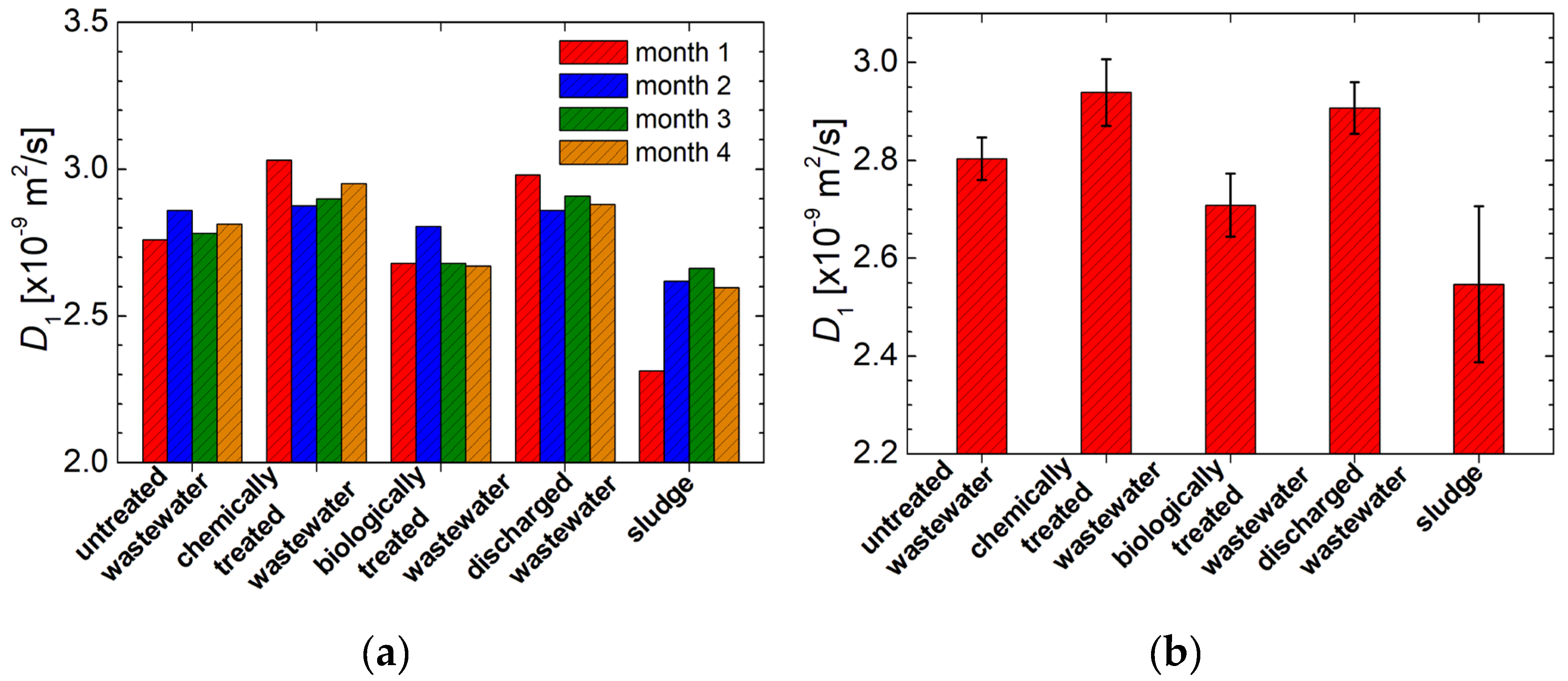
Figure 10.
(a) The total absorbance of VIS-nearIR spectra recorded for the slaughterhouse wastewater (untreated, chemically treated, biologically treated and discharged water) and sludge collected in all four months of monitoring; (b) The averaged of total absorbance of VIS-nearIR spectra of wastewater and sludge presented in (a).

Figure 11.
(a) The pH measured for the slaughterhouse wastewater (untreated, chemically treated, biologically treated and discharged wastewater) and sludge collected in all four months of monitoring; (b) The averaged pH over months measured for all four wastewater and sludge samples presented in (a).
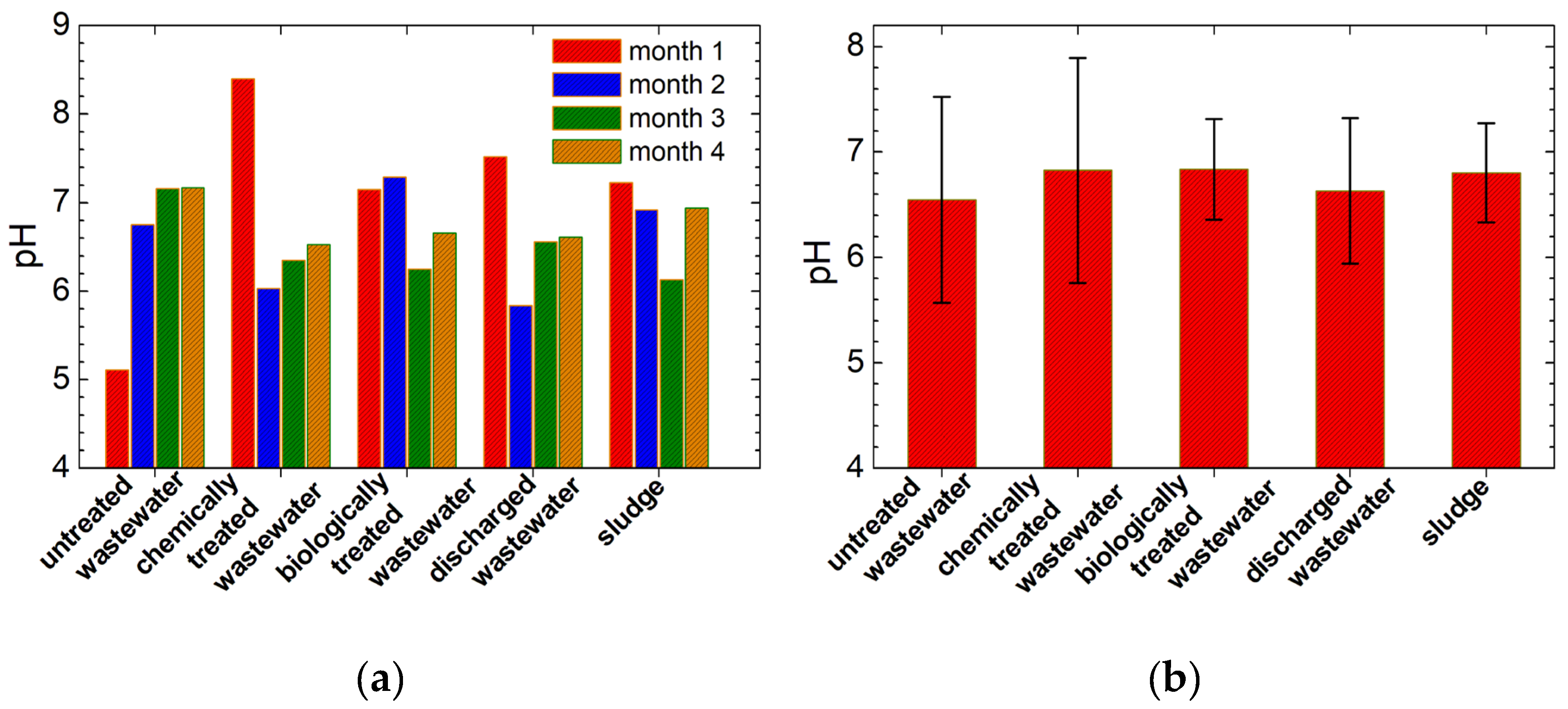
Figure 12.
(a) The electric conductivity (EC) measured for the slaughterhouse wastewater (untreated, chemically treated, biologically treated and discharged wastewater) and sludge collected in all four months of monitoring; (b) The averaged EC over months measured for all wastewater and sludge presented in (a).
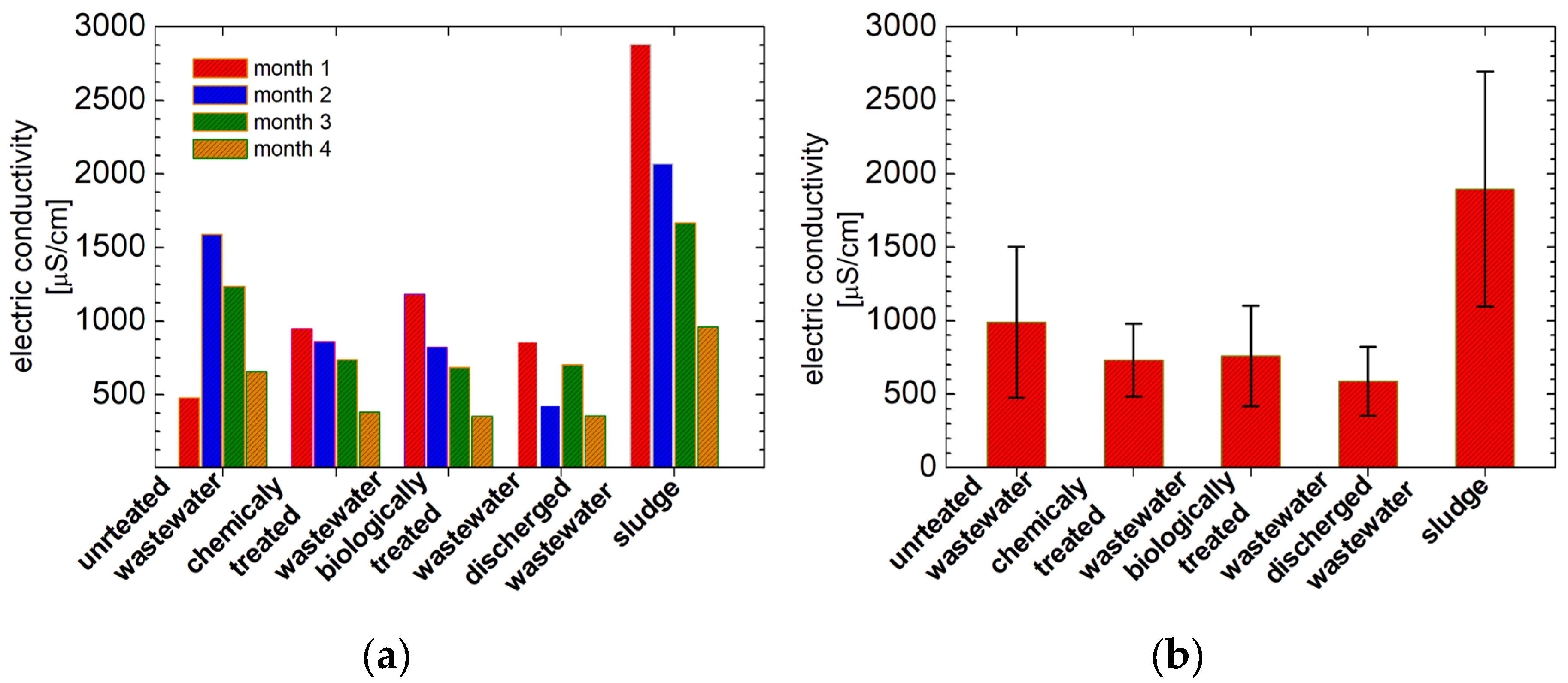
Figure 13.
(a) The total dissolved solid (TDS) measured for the slaughterhouse wastewater (untreated, chemically treated, biologically treated and discharged wastewater) and sludge samples collected in all four months of monitoring; (b) The averaged TDS measured for all wastewater and sludge samples presented in (a).
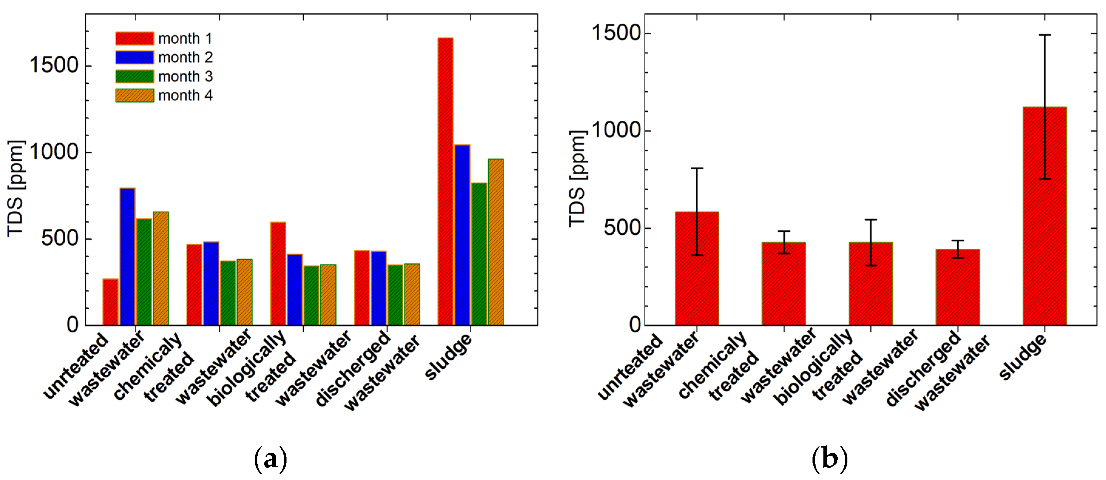
Figure 14.
The main PCA analysis: the 2D plot of PC1 function of PC2 for the slaughterhouse wastewater (untreated, biologically treated, chemically treated and discharged wastewater) and sludge samples collected in all four months of monitoring.
Figure 14.
The main PCA analysis: the 2D plot of PC1 function of PC2 for the slaughterhouse wastewater (untreated, biologically treated, chemically treated and discharged wastewater) and sludge samples collected in all four months of monitoring.
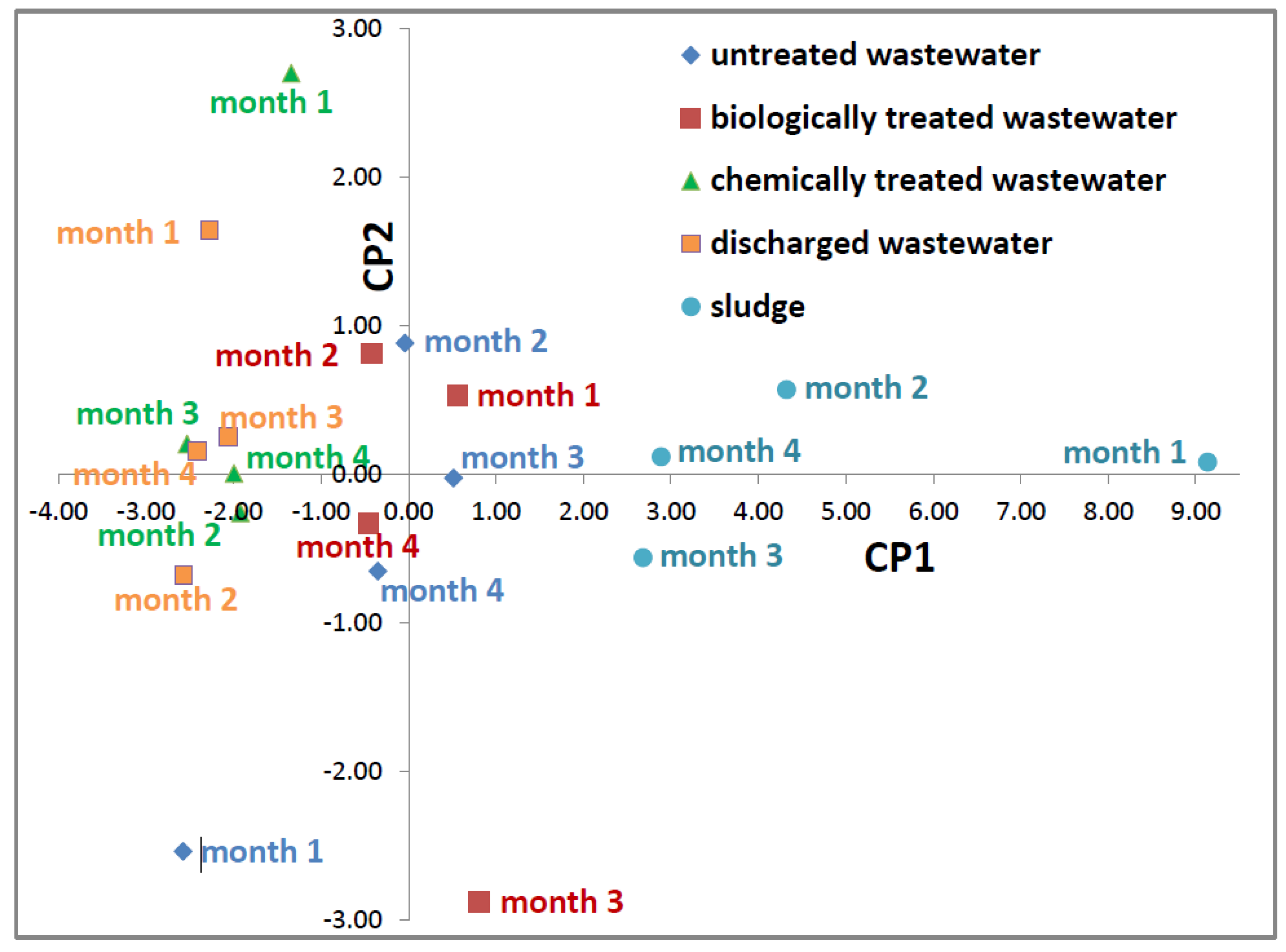
Figure 16.
The predicted probability using ANN for a) the untreated wastewater, b) chemically treated wastewater c) biologically treated wastewater d) discharged wastewater and e) sludge.
Figure 16.
The predicted probability using ANN for a) the untreated wastewater, b) chemically treated wastewater c) biologically treated wastewater d) discharged wastewater and e) sludge.
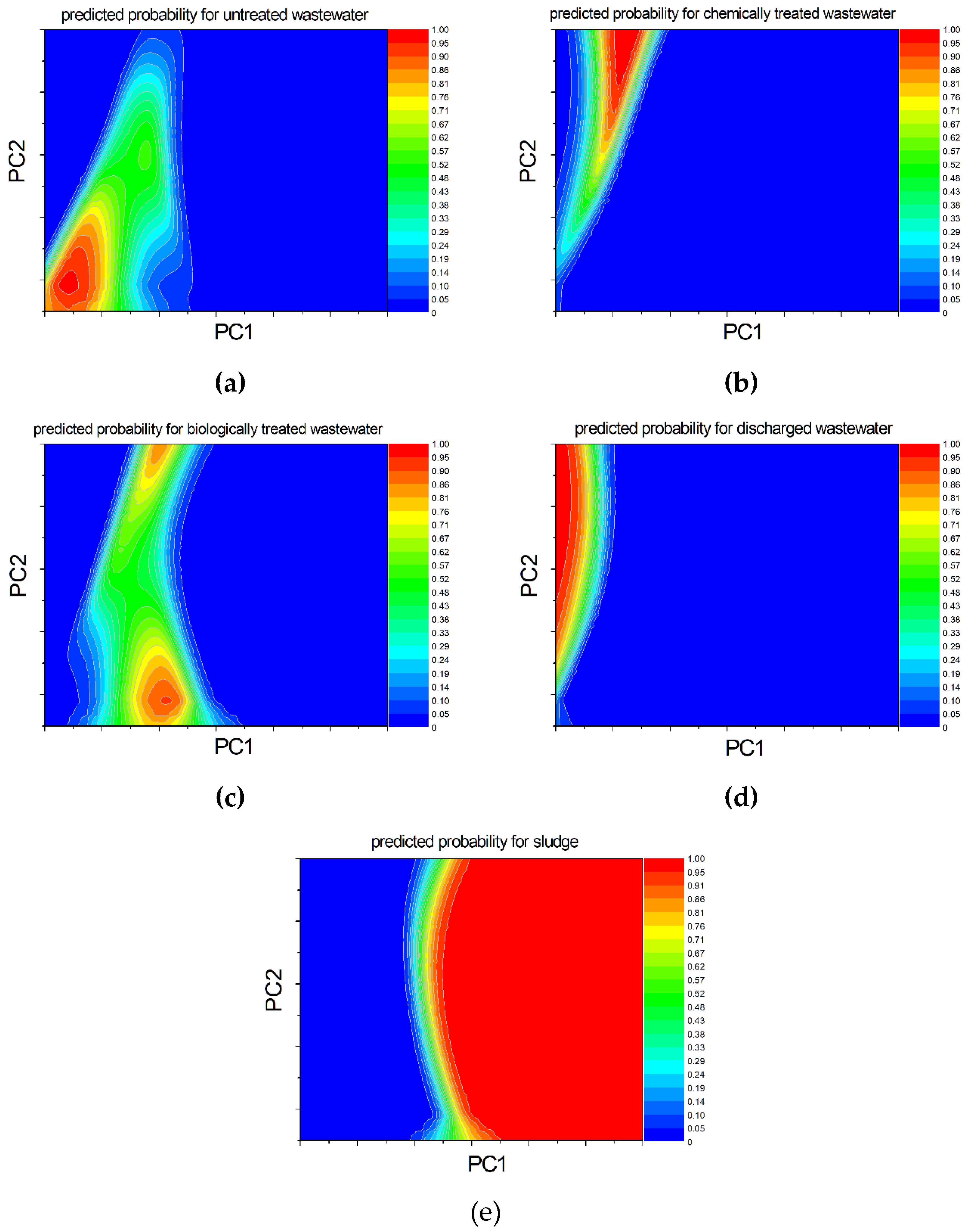
Table 2.
The contribution of relevant parameters (total VIS-nearIR absorbance, the most probable transverse relaxation time T2,1, the self-diffusion coefficient D1, pH, electric conductivity EC and the total dissolved solids TDS) measured for the slaughterhouse wastewater to the principal components PC1–PC6.
| parameter | PC1 | PC2 | PC3 | PC4 | PC5 | PC6 |
|---|---|---|---|---|---|---|
|
total VIS-nearIR absorbance |
0.336 | -0.627 | 0.550 | 0.430 | -0.079 | -0.025 |
| T2,1 [s] | -0.561 | 0.054 | 0.703 | -0.417 | 0.117 | 0.026 |
| D1 [10-9 m2/s] | -0.892 | 0.343 | 0.122 | 0.036 | -0.244 | -0.104 |
| pH | 0.250 | 0.794 | 0.264 | 0.478 | 0.085 | 0.032 |
| EC [μS/cm] | 0.884 | 0.220 | 0.173 | -0.288 | -0.211 | 0.118 |
| TDS [ppm] | 0.933 | 0.165 | 0.107 | -0.226 | 0.042 | -0.195 |
In all cases the measurement errors are smaller than 5%.
Disclaimer/Publisher’s Note: The statements, opinions and data contained in all publications are solely those of the individual author(s) and contributor(s) and not of MDPI and/or the editor(s). MDPI and/or the editor(s) disclaim responsibility for any injury to people or property resulting from any ideas, methods, instructions or products referred to in the content. |
© 2024 by the authors. Licensee MDPI, Basel, Switzerland. This article is an open access article distributed under the terms and conditions of the Creative Commons Attribution (CC BY) license (http://creativecommons.org/licenses/by/4.0/).
Copyright: This open access article is published under a Creative Commons CC BY 4.0 license, which permit the free download, distribution, and reuse, provided that the author and preprint are cited in any reuse.


