Submitted:
01 July 2024
Posted:
01 July 2024
You are already at the latest version
Abstract
To address the issue of reduced orbit estimation accuracy resulting from discrepancies between in-orbit measured geomagnetic field values and IGRF model values in autonomous orbit estimation of microsatellites based on geomagnetic field measurements, this study introduces an adaptive cubature H-infinity filtering algorithm. Firstly, it presents the low-altitude orbital dynamics model and geomagnetic field measurement model for microsatellites. Subsequently, within the adaptive cubature H-infinity filtering algorithm, a spherical simplex rule and a second-order Gaussian-Legendre quadrature criterion are employed to compute the spherical surface integral and radial integral. Additionally, a spherical simplex-radial quadrature rule is proposed to enhance the approximation accuracy of nonlinear Gaussian weighted integrals. Furthermore, by integrating extended H-infinity filtering based on game theory with the cubature quadrature rule, an inverse proportional relationship between constraint level and filtering innovation is established. This allows for adaptive adjustment of the constraint level to enhance robustness against model errors. Finally, through semi-physical simulation experiments, it is demonstrated that compared with traditional algorithms, the proposed algorithm improves autonomous orbit estimation position accuracy of microsatellites by 7.49%, while also enhancing velocity accuracy by 3.1%, thus validating its effectiveness.
Keywords:
autonomous orbit estimation
; microsatellite
; cubature Kalman filter
; robust
; geomagnetic field
1. Introduction
The autonomous navigation of microsatellites pertains to the technology for real-time determination of the position and velocity of microsatellites without reliance on ground support, utilizing solely the onboard measurement equipment. With the proliferation of space programs across different nations, there has been a surge in the number of micro-satellites operating in low Earth orbit, enhancing space application capabilities while imposing significant demands on ground telemetry and control systems. To mitigate the dependence of microsatellites on ground telemetry and control and enhance their autonomous intelligent operation in orbit, as well as serving as an effective complement to traditional ground telemetry and control, research into autonomous orbit determination technology for microsatellites has emerged as a pivotal focus within the realm of microsatellite technology [1,2,3].
The autonomous orbit determination method for microsatellites can be categorized into three main approaches: astrometric navigation orbit determination based on celestial measurements, autonomous navigation orbit determination based on beacon measurements, and geodetic/geographic information matching navigation orbit determination. The first approach involves measuring the position of known natural celestial bodies relative to the microsatellite and then estimating the orbital parameters using the least squares method based on the orbital dynamics model [4]. The second approach relies on signals received from beacons located at various positions with a specific pattern, enabling estimation of the orbital parameters through measured relative distances and rate of change using an orbital dynamics model [5]. The third approach utilizes onboard instruments such as optical imaging sensors, magnetometers, or gravity gradiometers to obtain measurement information related to geophysical fields or Earth's surface features for estimating orbital parameters by matching them with a prior model [6,7]. Geomagnetic navigation is particularly suitable for medium-low precision orbit determination of near-earth micro-satellites due to abundant magnetic field resources in near-earth orbits that can be described by Gaussian spherical harmonics [8,9]. The intensity and direction of the magnetic field can be expressed as a function of satellite position, making it feasible to use magnetic measurement methods for autonomous satellite orbit determination if a magnetometer meets requirements such as light weight, low power consumption, high reliability, and low cost.
The autonomous orbit estimation of a small satellite based on geomagnetic field measurements presents a fundamental nonlinear filtering challenge. Commonly employed solutions include the extended Kalman filter (EKF) [10], the unscented Kalman filter (UKF) [11,12,13], and the cubature Kalman filter (CKF) [14,15]. Among these, the EKF's use of first-order Taylor expansion compromises filtering accuracy. The UKF approximates the distribution of the nonlinear function using a set of sigma points, thereby enhancing estimation accuracy. However, its parameter selection lacks clear theoretical basis and may yield negative weights for variable dimensions exceeding 3, potentially leading to non-positive definite covariance matrices that directly impact estimate stability. The CKF decomposes the nonlinear Gaussian weighted integral into spherical surface and radial integrals, utilizing an equal-weighted set of cubature points to achieve superior filtering accuracy and numerical stability compared to EKF and UKF, making it widely applicable in engineering [16,17,18]. During application, filters often encounter model error and imprecise statistical noise characteristics; robustness refers to a filter's ability to withstand such challenges. The H-infinity filter is designed with improved robustness in mind addresses conservative filtering due to fixed constraint levels by proposing an adaptive robust filtering algorithm that comprehensively considers filter performance [19]. Furthermore, Ref. [20] designs a robust filtering algorithm capable of improving system adaptability to changing model parameters while addressing difficulties in precise modeling and unobtainable noise statistical characteristics. Ref. [21] combines H-infintiy filtering with CKF algorithms to propose a nonlinear robust filtering algorithm aimed at enhancing system robustness against abnormal observation values.
This paper presents an adaptive cubature H-infinity filtering algorithm. Firstly, it provides the low-altitude orbital dynamics model and the Earth's magnetic field measurement model of a small satellite. Subsequently, in the context of the adaptive cubature H-infinity filtering algorithm, on one hand, the spherical integral and radial integral are computed using the spherical simplex criterion and the second-order Gaussian-Legendre quadrature criterion respectively. The spherical simplex-radial cubature quadrature rule is then introduced to enhance the approximation accuracy of nonlinear Gaussian weighted integrals. On the other hand, game theory-based extended H-infinity filtering is integrated with the cubature rule to establish an inverse relationship between constraint level and filtering innovation. The constraint level is adaptively adjusted to improve robustness against model errors within this algorithm framework. Finally, a semi-physical simulation experiment demonstrates the effectiveness of this proposed algorithm.
The remainder of this paper is organized as follows: the autonomous orbit estimation models are described in Section 2, the adaptive robust cubature H-infinity filter is deduced in Section 3, the semi-physical simulation and results are presented in Section 4, and the conclusions are drawn in Section 5.
2. Autonomous Orbit Estimation Models
2.1. Dynamics Model of Low Orbit
For satellites in low Earth orbit, the primary perturbations experienced by the satellite in the Earth-fixed coordinate system () are the non-spherical Earth term and atmospheric drag. When considering these perturbations, the orbital dynamics model of the satellite is as follows:
where , , represent the position vector and velocity vector of the microsatellite in the , respectively. denotes the coefficient of the harmonic term, signifies the gravitational constant of the Earth, stands for the Earth's radius, and represents the Earth's rotational angular velocity. accounts for atmospheric drag perturbation, where denotes the atmospheric drag coefficient, represents the satellite's frontal area-to-volume ratio, and stands for atmospheric density. Assuming that the atmosphere rotates with the Earth, the relative velocity between a satellite and the atmosphere is expressed as , where is indicative of Earth's rotational angular velocity vector. encompasses third-order non-spherical perturbation summing with three-body perturbation and solar radiation pressure perturbation along all three coordinate axes.
In order to facilitate the implementation of the discrete Kalman filtering orbit determination algorithm on board a spacecraft computer, it is essential to discretize the continuous-time spacecraft orbital dynamics model presented in equation (1). In this study, we employ the classical fourth-order Runge-Kutta method as the discretization technique. For the continuous equation , its general numerical computation format is: ,,,,. Utilizing the fourth-order Runge-Kutta method enables us to express equation (32) in the following discrete form:
where denotes the orbital state at time k, signifies the non-linear functional relationship as depicted in equation (1), and represents the system noise.
2.2. Geomagnetic Field Measurement Model
The magnetometer offers the advantages of compact size, lightweight design, cost-effectiveness, reliable performance, and absence of field of view restrictions. It is capable of providing real-time continuous geomagnetic field measurement information in all weather conditions and is considered a fundamental component on current low-orbit microsatellites. The theoretical expression of the spherical harmonic model for the geomagnetic field elucidates that the primary source of the geomagnetic field lies within the Earth. The International Association of Geomagnetism and Aeronomy (IAGA) periodically releases a new iteration of the International Geomagnetic Reference Field (IGRF) every five years to furnish measurement data for ongoing refinement and enhancement of our understanding about the geomagnetic field. The potential function for the geomagnetic field can be represented as:
In this equation, represents the reference equatorial radius of the Earth, R denotes the geocentric distance, λ stands for geographic longitude, signifies geocentric colatitude, , and φ indicates geocentric latitude. refers to an nth-order mth-degree quasi-associated Legendre function, while and are denoted as the Gaussian coefficient. The IGRF model provides a table of corresponding Gaussian coefficients.
The geomagnetic field vector can be expressed as the negative gradient of the geomagnetic potential function as follows.
The relationship between the geomagnetic field vector and satellite position can be derived from equations (3) and (5). Specifically, the components of the geomagnetic field vector in the Earth-fixed coordinate system are as follows:
The higher the order of expansion for equation (6), the greater the model accuracy, and correspondingly, the greater the computational complexity. Let , then equation (6) can be expressed in the form of the following discrete measurement equation.
where represents the three-axis geomagnetic field measured at time k by the magnetometer, denotes the nonlinear model function describing the three-axis geomagnetic field on the right-hand side, and signifies the measurement noise of the magnetometer at time k.
3. Adaptive Robust Cubature H-Infinity Filter
3.1. Suboptimal Solution of the Extended H-Infinity Filter
Consider the discrete nonlinear dynamic system described by equations (2) and (7).
where we make the assumption that the system noise and the measurement noise are bounded energy signals with unknown statistical properties. Specifically, we impose the following constraints: , .
Let denote the mapping operation that associates the unknown perturbation, ,, , with the estimated error . Here, represents the initial state of the system, denotes its estimated value, and its variance reflects the approximation accuracy of to. Moreover, the objective of the H-infinity filter is to determine an estimation strategy such that minimizes the H-infinity norm of this operation . The H-infinity norm of this transfer operation is defined as:
In the equation, "sup" represents the supremum, and is a bounded signal, that is .
Nevertheless, in certain exceptional scenarios, closed-form solutions for the optimal H-infinity filtering can be derived, wherein a cost function is stipulated [22].
where and are weight matrices that can be adjusted based on performance requirements. In practical applications, and can be regarded as estimations of the corresponding noise covariance matrices, with a norm .
The H-infinity filtering problem aims to minimize the normalized energy of the estimation error under various conditions, while also minimizing the energy of the input noise and initial error, thus satisfying:
where represents a predetermined threshold value known as the constraint level.
An analytical solution for suboptimal H-infinity filtering based on Krein space Kalman filtering, which is a suboptimal filter compared to the standard Kalman filter, differs from the latter primarily in the computation of the posterior covariance matrix. In suboptimal H-infinity filtering, the method for computing the posterior covariance matrix is as follows:"
It is evident that the covariance matrix of the extended H-infinity filter (EH∞F) incorporates an additional regulating term in comparison to the covariance matrix of the standard Kalman filter. The iterative calculation steps for the EH∞F algorithm are as follows:
Compute the prior state estimation;
Compute the prior error covariance matrix;
Calculate the inverse of the posterior error covariance matrix;
Compute the posterior state estimation;
Determine the Kalman filter gain matrix.
where and denote the Jacobian matrices evaluated at and , respectively.
It is evident that the EH∞F exhibits a computational structure akin to that of the EKF, particularly when . As such, the EH∞F simplifies to the EKF. Consequently, the EH∞F can be considered a more general algorithm, with serving as a tuning parameter that balances robustness and precision in control algorithms.
3.2. Adaptive Determination of Constraint Level Values
The degree of constraint significantly influences the accuracy and robustness of the filtering process. Traditionally, it is assigned a fixed value based on engineering experience, leading to conservative filter performance. To strike a balance between filtering accuracy and robustness, an adaptive optimization approach should be employed.
To incorporate the EH∞F into the CKF computation framework, it is essential to adopt the following linear error propagation principle for approximating the measurement error covariance matrix and cross-error covariance matrix, . Subsequently, the measurement update step of the cubature H∞ filter is computed as follows:
The inverse matrix of the posterior error covariance matrix for EH∞F is derived as follows.
The constraint level directly impacts the robust filter's performance. A smaller value enhances system robustness but reduces filtering accuracy, while a larger value compromises system stability and may lead to divergence. The selection of the constraint level must satisfy the following Riccati inequality.
To achieve the adaptive selection of the constraint level , we initially introduce the following lemma.
Lemma 1. [23] Suppose A and B are two n-order Hermitian matrices, ,, and then ,where represents the maximum eigenvalue.
The square of the filter innovation can be utilized to denote the actual estimation error of the filter. A large value of indicates poor system stability, necessitating a reduction of to enhance filter robustness. Conversely, a small value signifies high estimation accuracy, allowing for an increase in to reduce the need for filter robustness. Thus, there exists an inverse relationship between the constraint level and .
The formula (15) is written in the following equivalent form:
After defining the matrix , we obtain , and according to Lemma 1, we have , thus enabling us to establish:
where , as there exists an inverse proportional relationship between and , let
where represents the phase relationship coefficient, typically determined through experimental means. Once is established, the coefficient becomes solely dependent on the new information filter, effectively quantifying the relationship between and .
3.3. Adaptive H-Infinity Filtering Algorithm with Adjustable Constraint Level
3.3.1. Spherical Simplex-Radial Cubature Quadrature Rule
Given the integral , let , where , satisfies represents the surface of the unit sphere, and is the radius of the sphere. Then can be decomposed into a spherical surface integral and a radial integral; however, obtaining analytical solutions for these integrals is generally challenging. Therefore, numerical approximation methods are considered. According to [24], a three-order spherical simplex rule consisting of points can be used to approximate the spherical surface integral as follows:
where represents the surface area of the n-dimensional unit sphere, while , denote the set of vertices of the n-dimensional simplex, with their elements defined as follows:
For the radial integral, let , resulting in . Subsequently, we have . Set ,and we obtain . This approach enables us to approximate the integral term using the Gauss-Laguerre quadrature rule [25] as follows.
where denotes the integration points, while represents the corresponding weights. The integration points can be derived from the solutions of p-th order Chebyshev-Laguerre polynomials as follows.
The corresponding weights can be derived by solving the following equation.
where the Gamma function is utilized. The approximate precision of this rule relies on the number of points employed for integration, and for , the subsequent approximation can be derived.
Solving equations (22) and (23) yields the values of ,, and as follows:
The essence of the nonlinear Kalman filter lies in the computation of the Gaussian weighted integral . Here, represents the Gaussian probability density function. The integral takes on the following identity form:
By combining equation (24) with ,,, we can derive the following spherical simplex-radial cubature quadrature rule for calculating as follows :
In particular, when the condition in Equation (21) is met , we can solve for , , and subsequently derive the spherical simplex-radial cubature quadrature rule as presented in the literature [24]. This demonstrates that the proposed spherical simplex-radial cubature quadrature rule in this paper exhibits higher accuracy than the previously established spherical simplex-radial cubature rule.
The represents the matrix composed of , is used to represent the i-th column of the matrix, using formula (27) to construct the cubature points and weights as follows:
3.3.2. Adaptive H-Infinity Filter with Constrained Level Adjustment
In this paper, based on the system model equation (2), it is evident that n equals 6. Substituting this value into the equations (28) and (29) yields the cubature points and corresponding weights as follows:
The specific calculation steps for cubature H-infinity filtering with adaptive constraint level adjustment are provided, incorporating an adaptive adjustment algorithm for the constraint level.
Step 1: Filter initialization.
Given the initial values of the filter ,,;
In the context of recursion, , complete the subsequent recursive update
Step 2: Time update.
Compute the cubature points by utilizing the preceding orbital state at time k-1 and the prior error covariance as .
Determine the non-linear transfer points of orbital states.
Compute the prior estimation of the orbital state at time k as.
Calculate the prior error covariance matrix for orbital state as;
Step 3: Measurement Update
Individually, utilize and to calculate the cubature points in accordance with the specified cubature criteria as .
Determine the non-linear transfer points of orbital states as.
Calculate the predicted measurement of magnetometer as.
Compute the matrix of measurement error covariance.
Compute the cross-covariance matrix. .
Compute the matrix of Kalman filter gain ;
Utilize the magnetic field measurements obtained from the magnetometer at time k to refine the posterior estimation of the computed state.
Compute the posterior error covariance matrix for the orbital state.
Step 4: Adaptive calculation of the level value constraint
Conduct iterative recursive computations of the value based on equations (17) and (18).
4. Simulation and Results
A semi-physical simulation experiment system for autonomous orbit determination of micro-satellite magnetic field has been established, as depicted in the figure. The experimental setup primarily comprises a micro-satellite simulator, a magnetic field coil, an air bearing turntable, a high-pressure air compressor, and relevant upper-level computer software. The magnetic field coil is capable of generating a desired strength magnetic field, and various disturbances can be introduced to simulate the in-orbit conditions of the micro-satellite as realistically as possible.
Figure 1.
Microsatellite Autonomous Orbit Estimation Semi-physical Simulation Experiment System; (a) Micro-satellite Simulator and Earth Magnetic Field Coil; (b) Complementary Parts.
Figure 1.
Microsatellite Autonomous Orbit Estimation Semi-physical Simulation Experiment System; (a) Micro-satellite Simulator and Earth Magnetic Field Coil; (b) Complementary Parts.
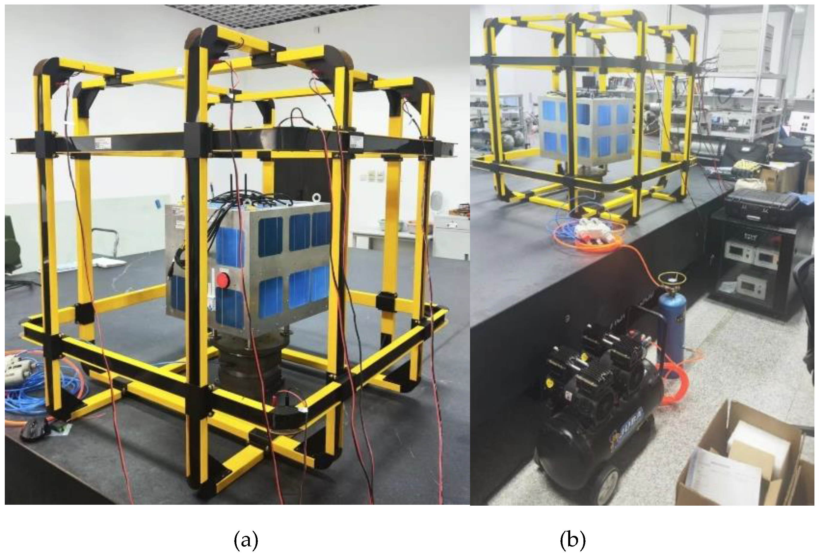
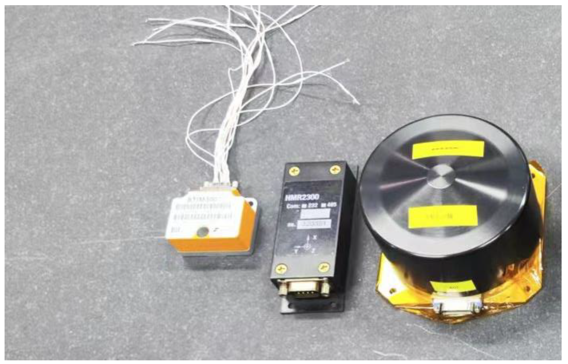
The micro-satellite simulator is equipped with a magnetometer to measure the magnetic field strength generated by the magnetic field coil, as depicted in the figure. Additionally, it incorporates a star sensor and gyroscope for attitude determination, along with a flywheel and a magnetic torque device for attitude control. The simulator utilizes the HPOP (High Precision Orbit Propagation) orbit prediction algorithm to run tests, accounting for perturbations such as atmospheric drag, solar pressure, and three-body gravity. The reference orbit's epoch is 1 Jun 2024 16:32:00 (UTCG), with a semi-major axis of 6878.137 km, eccentricity of 0, inclination of 97.035°, right ascension of the ascending node at 279.135°, argument of perigee at 0°, and true anomaly at 0°. The magnetometer boasts a measurement accuracy of 167 nT.
Figure 2.
Magnetometer, gyroscope and flywheel.
The root mean square error (RMSE) of position and velocity is employed for the assessment of the autonomous orbit estimation. The RMSE is defined as follows:
where N denotes the number of Monte Carlo simulations, and velocity RMSE is defined analogously to equation (32).
The simulation results are presented in Figure 3 and Figure 4, demonstrating that the estimated RMSE of ACH∞F is smaller than that of CKF, indicating the superior resilience of ACH∞F against unmodeled errors and its enhanced filtering performance under such conditions. To quantitatively characterize the autonomous orbit estimation accuracy of the microsatellites, the average RMSE of orbit determination is statistically summarized in Table 1 over the time interval of 5000~18,000s. The comparison reveals a notable improvement in positioning accuracy and velocity accuracy by 7.49% and 3.1%, respectively, for ACH∞F as compared to the CKF algorithm.
5. Conclusions
In order to address the issue of reduced orbit estimation accuracy resulting from disparities between in-orbit measured geomagnetic field values and model values in autonomous orbit estimation of microsatellites based on geomagnetic field measurements, this paper proposes an adaptive cubature H-infinity filtering algorithm. Firstly, it presents the low-altitude orbital dynamics model and geomagnetic field measurement model for microsatellites. Subsequently, within the adaptive cubature H-infinity filtering algorithm, a spherical polyhedron criterion and a second-order Gaussian-Legendre quadrature criterion are utilized to compute the spherical integral and radial integral. Additionally, a spherical simplex-radial quadrature integration criterion is introduced to enhance the approximation accuracy of nonlinear Gaussian weighted integrals. Furthermore, by integrating extended H-infinity filtering based on game theory with the cubature criterion, an inverse proportional relationship between constraint level and innovation in filtering is established. This allows for adaptive adjustment of constraint level to enhance algorithm robustness against model errors. Finally, through semi-physical simulation experiments, it is demonstrated that compared with traditional algorithms, the proposed algorithm improves autonomous orbit estimation accuracy of position and velocity of microsatellites by 7.49% and 3.1%, thus validating its effectiveness.
Author Contributions
Formal analysis, Y.L.; investigation, X.Y. and Z.L.; software, L.L.; validation, Z.L. All authors have read and agreed to the published version of the manuscript.
Funding
This research was funded by National Natural Science Foundation of China, grant number 62005320.
Data Availability Statement
The data presented in this study are available upon request from the corresponding author.
Conflicts of Interest
The authors declare no conflicts of interest.
References
- Zhong, W.; Gurfil, P. Mean Orbital Elements Estimation for Autonomous Satellite Guidance and Orbit Control. J. Guid. Control. Dyn. 2013, 36, 1624–1641. [Google Scholar] [CrossRef]
- Shi, Y.; Wang, J.; Liu, C.; Wang, Y.; Xu, Q.; Zhou, X. Angle-Only Cooperative Orbit Determination Considering Attitude Uncertainty. Sensors 2023, 23, 718. [Google Scholar] [CrossRef] [PubMed]
- Cui, F.; Gao, D.; Zheng, J. Magnetometer-Based Orbit Determination via Fast Reconstruction of Three-Dimensional Decoupled Geomagnetic Field Model. J. Spacecr. Rocket. 2021, 58, 1374–1386. [Google Scholar] [CrossRef]
- Qian, H.-M.; Sun, L.; Cai, J.-N.; Huang, W. A starlight refraction scheme with single star sensor used in autonomous satellite navigation system. Acta Astronaut. 2014, 96, 45–52. [Google Scholar] [CrossRef]
- Xiong, K.; Wei, C.L.; Liu, L.D. Performance enhancement of X-ray pulsar navigation using autonomous optical sensor. Acta Astronautica 2016, 128, 473–484. [Google Scholar]
- Cheon, Y.-J. Fast convergence of orbit determination using geomagnetic field measurement in Target Pointing Satellite. Aerosp. Sci. Technol. 2013, 30, 315–322. [Google Scholar] [CrossRef]
- Tahir, M.; Moazzam, A.; Ali, K. A Stochastic Optimization Approach to Magnetometer Calibration With Gradient Estimates Using Simultaneous Perturbations. IEEE Trans. Instrum. Meas. 2018, 68, 4152–4161. [Google Scholar] [CrossRef]
- Cui, F.; Gao, D.; Zheng, J. Magnetometer-based autonomous orbit determination via a measurement differencing extended Kalman filter during geomagnetic storms. Aircraft engineering and aerospace technology, ahead-of-print(ahead-of-print). 2020. [Google Scholar]
- Wu, J.; Zhang, C.X.; Liu, M. Hybrid geomagnetic attitude and orbit estimation using time⁃differential feedback. Transactions of The Japan Society for Aeronautical&Space Sciences 2021, 64, 174–180. [Google Scholar]
- He, L.N.; Zhou, H.R.; Zhang, G.Y. . Improving extended Kalman filter algorithm in satellite autonomous navigation. Proceedings of Institution of Mechanical Engineers Part G: Journal of Aerospace Engineering 2017, 231, 743–759. [Google Scholar] [CrossRef]
- Julier, S.; Uhlmann, J.; Durrant-Whyte, H.F. A new method for the nonlinear transformation of means and covariances in filters and estimators. IEEE Trans. Autom. Control 2001, 45, 477–482. [Google Scholar] [CrossRef]
- Hu, G.; Xu, L.; Gao, B.; et al. Robust Unscented Kalman Filter-Based Decentralized Multisensor Information Fusion for INS/GNSS/CNS Integration in Hypersonic Vehicle Navigation. IEEE Transactions on Instrumentation and Measurement 2023, 72, 1–11. [Google Scholar] [CrossRef]
- Yang, W.; Li, S.; Li, N. A switch-mode information fusion filter based on ISRUKF for autonomous navigation of spacecraft. Inf. Fusion 2013, 18, 33–42. [Google Scholar] [CrossRef]
- Arasaratnam, I.; Haykin, S. Cubature Kalman filters. IEEE Transactions on Automatic Control 2009, 54, 1254–1268. [Google Scholar] [CrossRef]
- Arasaratnam, I.; Haykin, S.; Hurd, T.R. Cubature Kalman Filtering for Continuous-Discrete Systems: Theory and Simulations. IEEE Trans. Signal Process. 2010, 58, 4977–4993. [Google Scholar] [CrossRef]
- Haghparast, B.; Salarieh, H.; Pishkenari, H.N.; et al. A Cubature Kalman Filter for parameter identification and output-feedback attitude control of liquid-propellant satellites considering fuel sloshing effects. Aerospace science and technology 2024, 144, 108813.1–108813.9. [Google Scholar] [CrossRef]
- Potnuru, D.; Chandra, K.P.B.; Arasaratnam, I.; et al. Derivative-free square-root cubature Kalman filter for non-linear brushless DC motors. IET Electric Power Applications 2016, 10, 419–429. [Google Scholar] [CrossRef]
- Zhao, Y. Performance evaluation of Cubature Kalman filter in a GPS/IMU tightly-coupled navigation system. Signal Process. 2016, 119, 67–79. [Google Scholar] [CrossRef]
- Chatterjee, S.; Chowdhury, A.; Dey, A.; et al. Adaptive Divided Difference Filter for Power Systems Dynamic State Estimation With Outliers and Unknown Noise Covariance. IEEE Transactions on Industry Applications 2023, 6(Pt.2), 59. [Google Scholar] [CrossRef]
- Zhao, J.; Mili, L. Robust Unscented Kalman Filter for Power System Dynamic State Estimation with Unknown Noise Statistics. IEEE Transactions on Smart Grid 2017, 1–1. [Google Scholar] [CrossRef]
- Shao, J.; Zhang, Y.; Yu, F.; Fan, S.; Sun, Q.; Chen, W. A novel resampling-free update framework-based cubature Kalman filter for robust estimation. Signal Process. 2024, 221. [Google Scholar] [CrossRef]
- Garry, A.; Langford, B.W. Robust extended Kalman filtering. IEEE Transactions on Signal Processing 1999, 47, 2596–2598. [Google Scholar]
- Liu, X.; Hu, J.; Wang, H. Research on integrated navigation method based on adaptive H∞ filter. Chinese Journal of Scientific Instrument 2014, 35. [Google Scholar]
- Wang, S.; Feng, J.; Tse, C.K. Spherical Simplex-Radial Cubature Kalman Filter. IEEE Signal Process. Lett. 2013, 21, 43–46. [Google Scholar] [CrossRef]
- Bhaumik, S.; Swati, F. Cubature quadrature Kalman filter. IET Signal Processing 2013, 7, 533–541. [Google Scholar] [CrossRef]
Figure 3.
RMSE in three-dimensional autonomous orbit estimation. (a)Position RMSE in three directions; (b)Velocity RMSE in three directions.
Figure 3.
RMSE in three-dimensional autonomous orbit estimation. (a)Position RMSE in three directions; (b)Velocity RMSE in three directions.
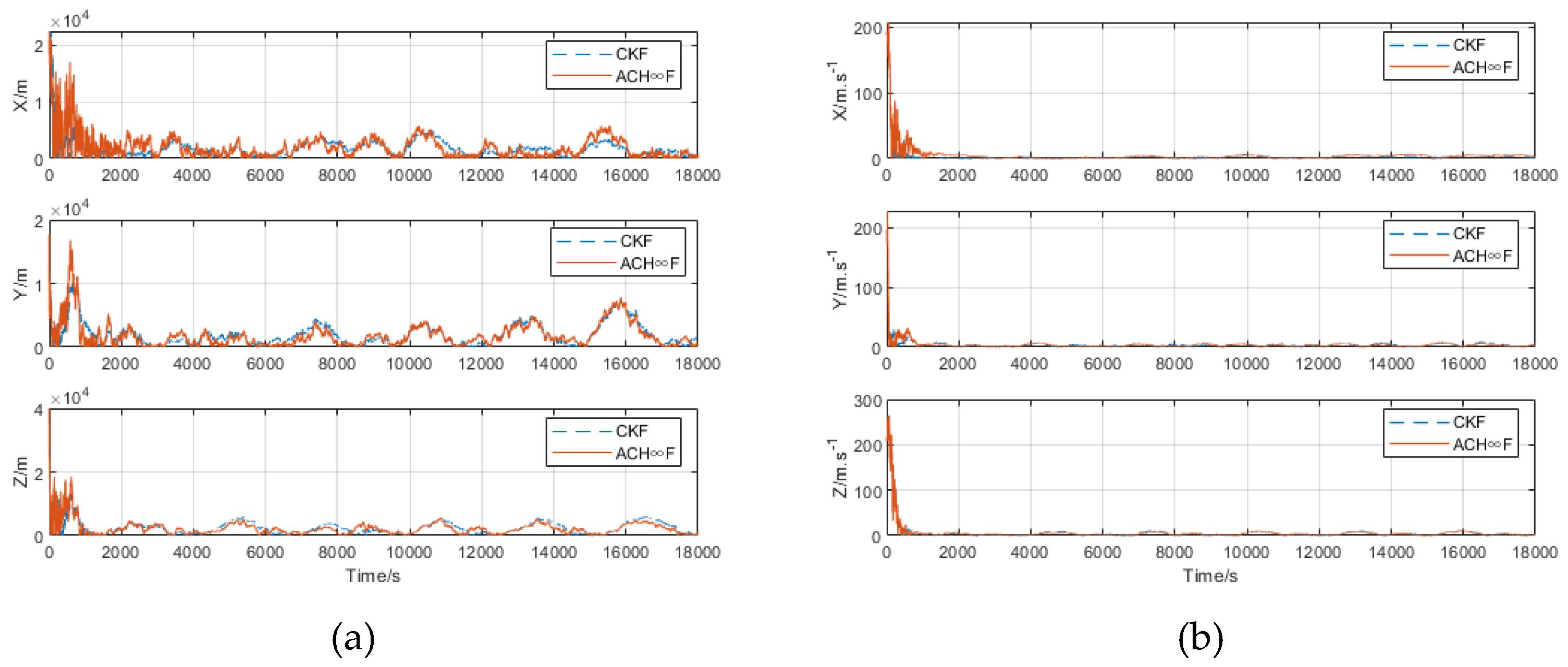
Figure 4.
RMSE for Autonomous Orbital Estimation. (a)Position RMSE; (b)Velocity RMSE.
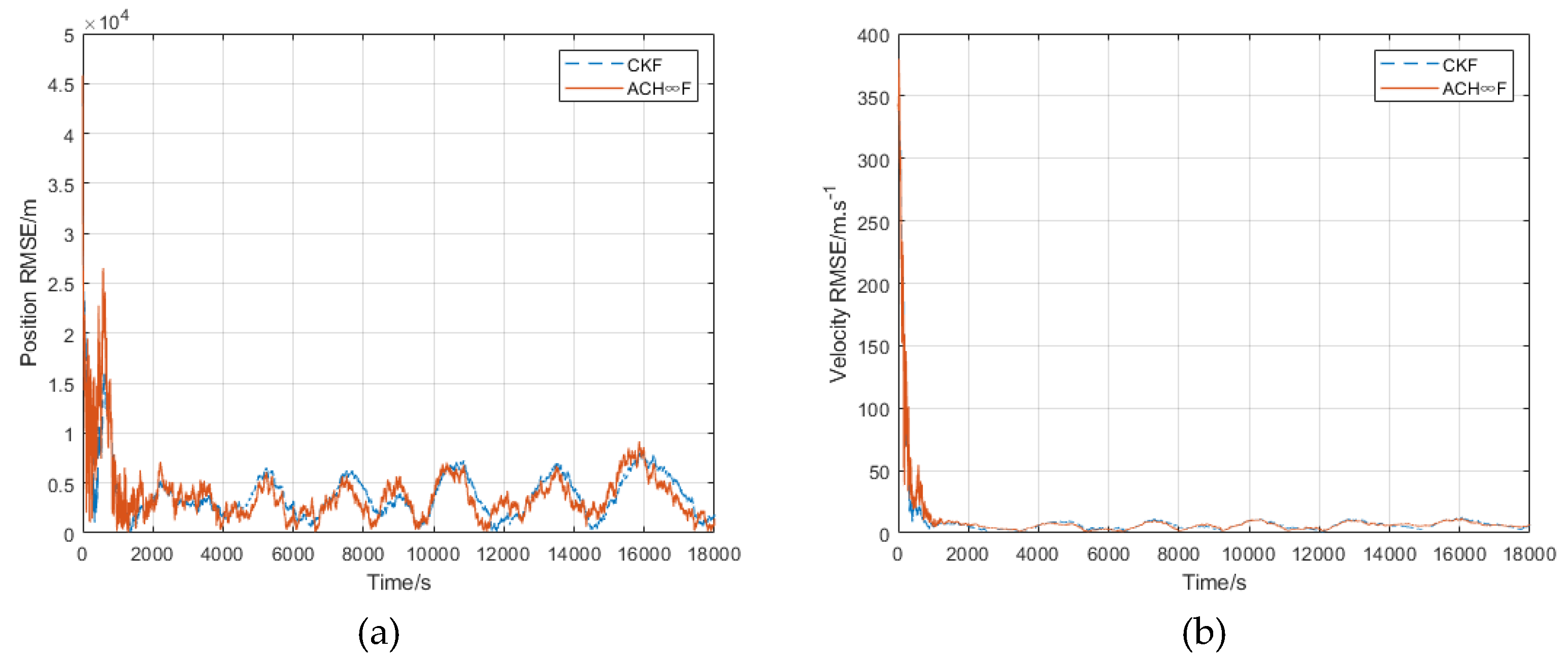

Table 1.
Two autonomous orbit estimation filtering algorithms with average RMSE.
| Filters | Average Positioning RMSE | Average Velocity RMSE |
|---|---|---|
| CKF | 3769.6 | 6.2005 |
| ACH∞F | 3487.3 | 6.0082 |
Disclaimer/Publisher’s Note: The statements, opinions and data contained in all publications are solely those of the individual author(s) and contributor(s) and not of MDPI and/or the editor(s). MDPI and/or the editor(s) disclaim responsibility for any injury to people or property resulting from any ideas, methods, instructions or products referred to in the content. |
© 2024 by the authors. Licensee MDPI, Basel, Switzerland. This article is an open access article distributed under the terms and conditions of the Creative Commons Attribution (CC BY) license (http://creativecommons.org/licenses/by/4.0/).
Copyright: This open access article is published under a Creative Commons CC BY 4.0 license, which permit the free download, distribution, and reuse, provided that the author and preprint are cited in any reuse.


